1. Introduction
Shear-induced migration is a conspicuous example of the effects of irreversible dynamics in shearing flows of Stokesian, non-colloidal suspensions. This irreversibility is somewhat puzzling since the flows are at low Reynolds numbers and the velocity field in the suspension is generally assumed to be governed by the linear, and reversible, Stokes equations. The irreversibility and resulting migration is due to the combined effects of hydrodynamic forces between the particles and non-hydrodynamic interactions. Close contact interactions, such as small roughness or short-ranged repulsive forces, can indeed lead to deviations of the particles from reversible trajectories (see e.g. Okagawa & Mason Reference Okagawa and Mason1973; Cunha & Hinch Reference Cunha and Hinch1996; Pine et al. Reference Pine, Gollub, Brady and Leshansky2005; Metzger, Pham & Butler Reference Metzger, Pham and Butler2013).
Shear-induced migration can drive particles, irreversibly, from the high to the low shear rate regions of the flow. This phenomenon was first clearly identified from experiments in a Couette viscometer by Leighton & Acrivos (Reference Leighton and Acrivos1987) and prompted a large number of experimental studies due to the impact that such migration has on the characterisation of suspension rheology. For pressure-driven flow through a pipe or channel, the particles migrate toward the centreline. The first evidence of such inhomogeneities in the suspension field dates back to Karnis, Goldsmith & Mason (Reference Karnis, Goldsmith and Mason1966). Since then, several experimental studies have been performed that measure migration in pressure-driven flows (Altobelli, Givler & Fukushima Reference Altobelli, Givler and Fukushima1991; Koh & Leal Reference Koh and Leal1994; Hampton et al. Reference Hampton, Mammoli, Graham, Tetlow and Altobell1997; Shauly et al. Reference Shauly, Averbakh, Nir and Semiat1997; Lyon & Leal Reference Lyon and Leal1998; Butler & Bonnecaze Reference Butler and Bonnecaze1999; Norman, Nayak & Bonnecaze Reference Norman, Nayak and Bonnecaze2005) using methods such as laser-Doppler velocimetry and magnetic resonance imaging. Most of these experiments have examined suspensions at large volume fractions, so that migration could be readily observable, and utilised neutrally buoyant particles. Additionally, most have reported measurements of the steady and fully-developed concentration and velocity profiles. Rather than steadily pumping the suspension, one can also use oscillatory flow. When the oscillation amplitude is large enough, migration toward the centre of the pipe is recovered; at small amplitudes, the particles migrate toward the wall (Butler, Majors & Bonnecaze Reference Butler, Majors and Bonnecaze1999; Morris Reference Morris2001).
Early efforts in modelling shear-induced migration utilised a diffusion model, in which gradients in the particle concentration, particle interaction frequency and effective suspension viscosity drive a diffusive flux of particles (Leighton & Acrivos Reference Leighton and Acrivos1987; Phillips et al. Reference Phillips, Armstrong, Brown, Graham and Abbott1992). The particle concentration field was derived by solving the diffusion equation in conjunction with the momentum equation for the suspension as a whole. This diffusion model successfully predicts the existence of migration in wide-gap Couette and pressure-driven Poiseuille flows, but fails to predict the absence of migration in curvilinear torsional flows (Chapman Reference Chapman1990; Chow et al. Reference Chow, Sinton, Iwamiya and Stephens1994; Krishnan, Beimfohr & Leighton Reference Krishnan, Beimfohr and Leighton1996; Bricker & Butler Reference Bricker and Butler2006).
A more recent and rather successful model relates the migration flux to the rheology of the suspension (Nott & Brady Reference Nott and Brady1994; Morris & Boulay Reference Morris and Boulay1999). This so-called suspension balance model (SBM) is a two-phase model which provides a continuum description of the bulk suspension motion, as well as the relative velocity of the particle phase and fluid phase. This model predicts that particle migration is driven by the divergence of the normal components of the particle phase stress (
 $\boldsymbol{{\rm\nabla}}\boldsymbol{\cdot }{\it\bf\Sigma}^{\boldsymbol{p}}$
), where
 ${\it\bf\Sigma}^{\boldsymbol{p}}$
comprises contact or interparticle contributions as well as hydrodynamic contributions coming from the non-drag portion of the interphase force (Lhuillier Reference Lhuillier2009; Nott, Guazzelli & Pouliquen Reference Nott, Guazzelli and Pouliquen2011). The SBM requires correlations for the particle phase stress which cannot be easily obtained experimentally.
Discrete particle simulations are another avenue to study inhomogeneities in suspension flows, wherein the motions of many discrete particles are calculated under the assumption that they are suspended in a Newtonian fluid. Such simulations of the pressure-driven flow in a two-dimensional channel of a suspension were conducted using Stokesian Dynamics (Nott & Brady Reference Nott and Brady1994). These simulations predicted migration in qualitative agreement with the experiments, while also demonstrating that shear-induced migration is not due to inertial effects, since Stokesian dynamics calculates flows in the limit of zero Reynolds number. Capabilities to simulate suspension flows have been expanding rapidly and providing enhanced information about migration. For example, three-dimensional numerical simulations of concentrated suspensions of
 $O(1000)$
monodisperse non-colloidal particles were performed recently in plane Poiseuille flows using the force coupling method (Yeo & Maxey Reference Yeo and Maxey2011).
The objective of the present work is to examine the dynamics of shear-induced migration in a pipe flow, in addition to the steady and fully developed concentration and velocity profiles which have been the focus of most previous studies. The experiments subject the suspension, consisting of neutrally buoyant spheres, to large oscillating displacements at low Reynolds number along the axis of the pipe, as described in § 2. Particle volume fraction and velocity are measured during the oscillations at high resolution by matching the refractive index of the fluid to that of the particles, and using fluorescence to distinguish the particle and fluid phases for imaging. Measurements of the shear-induced migration process are analysed and compared to previous experiments (Hampton et al. Reference Hampton, Mammoli, Graham, Tetlow and Altobell1997; Lyon & Leal Reference Lyon and Leal1998) as well as to the predictions of discrete particle simulations (Nott & Brady Reference Nott and Brady1994; Yeo & Maxey Reference Yeo and Maxey2011) in § 3. The results are also compared with predictions of the suspension balance model using realistic rheological laws; this model is detailed in the appendix A. Following Morris & Boulay (Reference Morris and Boulay1999), we use a phenomenological form for the normal stress of the particle phase, which has a viscous scaling and a similar concentration dependence in all directions. Two rheological models were tested: that of Morris & Boulay (Reference Morris and Boulay1999), which was chosen to match experimental results on migration, and that of Boyer, Guazzelli & Pouliquen (Reference Boyer, Guazzelli and Pouliquen2011a ), which was derived from pressure-imposed rheological measurements. A discussion and conclusions regarding the findings are given in § 4.
2. Experiments
2.1. Particles and fluids
Two sets of spheres composed of Poly(methyl methacrylate) with a density of
 $1.19~\text{g}~\text{cm}^{-3}$
were used in the experiments with diameters of
 $2a=2.01\pm 0.02~\text{mm}$
and
 $2a=1.05\pm 0.02~\text{mm}$
. Each diameter was determined by optically imaging more than 100 particles with the resulting measurements having an approximately Gaussian distribution. Analysis of the surface of the 2 mm particles by atomic force microscopy gives an r.m.s. and peak roughness of
 $0.06\pm 0.03~{\rm\mu}\text{m}$
and
 $0.6\pm 0.3~{\rm\mu}\text{m}$
, respectively; the surface properties of the 1 mm particles were not measured, but are expected to be similar. The suspending fluid, composed of
 $\text{ZnCl}_{2}$
(14.7 wt%), water (9.1 wt%) and Triton X-100 (76.2 wt%), was chosen to match the density and refractive index of the spheres. The fluid mixture was Newtonian, with a viscosity of
 ${\it\eta}_{f}=2.43~\text{Pa}~\text{s}$
at
 $27\,^{\circ }\text{C}$
. Approximately 3 ml of HCl was added for every 700 ml of suspending fluid in order to inhibit precipitation of
 $\text{ZnCl}_{2}$
. Additionally, rhodamine was added to the suspending fluid (
 ${\approx}6\times 10^{-7}~\text{g}~\text{cm}^{-3}$
) to aid in particle visualisation.
The suspensions were carefully prepared to avoid entrapping air in the highly viscous suspending fluid. The required quantity of spheres were added to the surface of the suspending fluid, both items being weighted to obtain the proper volume fraction. After the spheres were immersed in the fluid, the suspension was mixed by slowly stirring with a metal spatula and slowly rotating the beaker at an angle. This well mixed suspension was then added to the glass tube. Further mixing inside the glass tube prior to each experiment was performed as part of the experimental procedure.
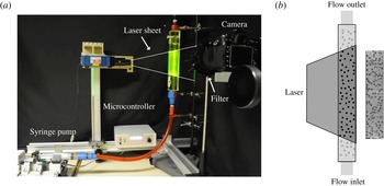
(a) The experimental apparatus is shown in the temperature controlled environment. (b) The laser sheet, rhodamine dye and long pass filter enable visualisation of the spherical particles, as shown in the diagram next to the raw experimental image.

2.2. Experimental apparatus
A photograph of the experimental apparatus is presented in figure 1(a). The suspension was oscillated in a circular glass tube of length 46.8 cm and diameter
 $2R=1.65~\text{cm}$
; for the two particle sizes used in the study, this gives geometric ratios of
 $R/a=8.21$
and
 $R/a=15.71$
. The tube was oriented vertically and a screen was placed at the entrance and exit of the glass tube to retain the particles within the tube, as the fluid pumped into the tube did not contain particles. A rectangular Plexiglas chamber surrounded the tube and the space between the chamber and the tube was filled with the suspending fluid. The housing and index-matched fluids reduce the optical distortion due to the curvature of the tube.
A syringe pump, connected to the glass tube by a flexible hose, and a microcontroller system generated an amplitude-controlled, oscillatory displacement of the suspension. The rate of volumetric displacement,
 $Q(t)$
, was applied as a square, rather than sinusoidal, wave as a function of time
 $t$
,
 $$\begin{eqnarray}Q(t)=({\it\gamma}R)({\rm\pi}R^{2})\frac{{\it\omega}\cos ({\it\omega}t)}{|\cos ({\it\omega}t)|},\end{eqnarray}$$
where the brackets
 $|\cdot |$
indicate the absolute value and the frequency
 ${\it\omega}$
was restricted to values which maintained the particle Reynolds numbers below
 $3.3\times 10^{-5}$
and the Péclet numbers above
 $4.3\times 10^{9}$
. The linear displacement of
 ${\it\gamma}R$
was set to be large relative to the tube radius in order to observe migration, but was also kept small compared to the length of the tube to avoid end effects. The dimensionless quantity
 ${\it\gamma}$
is equivalent to one-fourth of the strain amplitude as evaluated at the wall of the tube, but only for a fluid with a uniform viscosity distribution. All results are reported in terms of the strain amplitude,
 ${\it\gamma}$
, and the dynamics is reported in terms of the accumulated strain rather than time, since the frequencies were sufficiently low to ensure that the experiments were performed in the creeping flow regime. The accumulated strain is defined as
 $4N{\it\gamma}$
, where
 $N$
is the number of oscillations. The strain amplitude was
 ${\it\gamma}=5.4$
in all experiments reported in § 3, unless noted otherwise.
Figure 1(a) also shows the key elements of the imaging system. A laser sheet was produced by a Coherent Lasiris Green PowerLine Laser (wavelength 532 nm) and was passed through a mask attached to the apparatus. The mask had a precisely cut 1 mm slit and was positioned so that the laser sheet was only applied to the centre of the tube. The rhodamine dye in the suspending fluid fluoresced due to the applied laser. A Nikon D300s with an AF-S Micro Nikkor 60 mm
 $f/2.8$
G ED was used for imaging and a 590 nm red long pass filter was placed between the tube and the camera to enhance the contrast between the particles and the suspending fluid. The laser sheet and tube are illustrated in figure 1(b), together with an example image. To reduce photobleaching of the suspending fluid, a shutter was added to the laser. Both the shutter and the digital camera were actuated by the same microcontroller that operates the syringe pump.
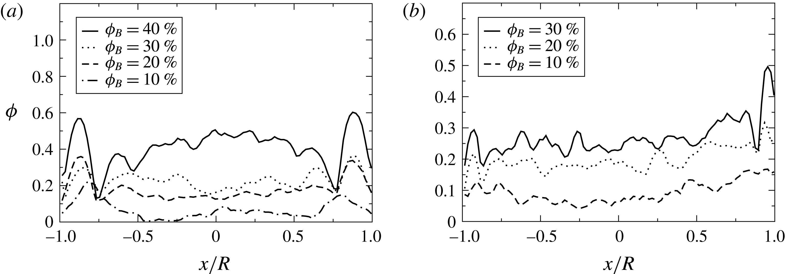
Examples of the initial particle distributions are shown for different bulk volume fractions at (a)
 $R/a=8.21$
and (b)
 $R/a=15.71$
.

2.3. Experimental procedure
Prior to each experiment, the suspension was mixed inside the glass tube using a long wire with impellers attached at various heights. After mixing, the suspension was held stationary for approximately one hour to remove any air. Examples of the initial volume fraction distribution are shown in figure 2(a,b), where
 ${\it\phi}$
is the local particle volume fraction,
 ${\it\phi}_{B}$
is the bulk particle volume fraction and
 $x$
is the horizontal position with the origin at the centre of the cylinder. The data analysis and averaging procedure used to produce these distributions are explained in the following section.
For each oscillation, forty images were recorded at one second intervals. The camera was adjusted to maximise the shutter speed while minimising the ISO and aperture used. This limited the noise to signal ratio while maintaining a shallow depth of field to ensure particles only in the laser sheet were imaged. Directly following the experiment, a ruler was photographed in order to properly scale the particle displacements. For a given bulk volume fraction and pipe-to-particle radius, several experiments were performed using exactly the same procedure as described above.
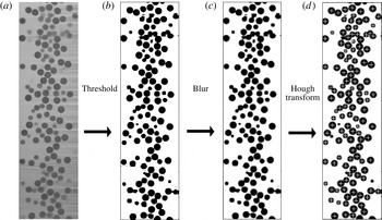
Examples of an image at each step in the particle velocity analysis. First the (a) raw image has a (b) histogram equalisation and threshold applied. Next, (c) a Gaussian blur and lastly a (d) circular Hough transform are used to locate the particle positions.

2.4. Data analysis
Images were analysed to obtain the particle volume fraction and velocity distributions. The accuracy in measuring these two different properties depends on identifying two different characteristics in the analysed images: (i) distinguishing an individual particle or (ii) maintaining the particle shape. Consequently, two different analyses were required.
Calculation of the particle volume fraction distribution required several steps of image processing. First, an adaptive histogram equalisation method (MATLAB_R2012a function adapthisteq) was used. This method locally enhances contrast by matching the given domain histogram to a specified distribution. These domains are subsets of the total image and are connected through bilinear interpolation. The number and spacing of the domains and histogram distributions were set to distinguish the particles from the background. Next, a threshold was calculated (using MATLAB_R2012a function graythresh) which uses the Otsu method of assuming a bimodal histogram and calculates a threshold level by minimising the combined spread from the two classes. Then the image was filtered (using MATLAB_R2012a function in2bw) by assigning pixel values greater than the calculated threshold as white, and the rest as black. Examples of an image before and after applying the threshold are displayed in figure 3(a,b). The volume fraction was calculated from the resulting binary images by treating black pixels as particles and white pixels as suspending fluid. To average across experiments, columns of pixels were assigned to a bin and the average volume fraction in the bin was calculated. Both dynamic and steady-state results were averaged across experiments, where the number of bins and the images used for averaging will be stated in the text.
The previous steps were also used to measure the particle velocity, but the specified parameters were optimised to distinguish individual particles. This required erosion of the particles, which would lead to an incorrect calculation of the volume fraction. After using the adaptive histogram equalisation and thresholding techniques to distinguish the particles, a Gaussian blur was applied, followed by a circular Hough transform to calculate the particle positions. Examples of the results are shown in figure 3(c,d). The Hough transform uses gradients in pixel values and a specified maximum and minimum radius to locate the particle positions. The maximum and minimum particle radii were chosen to approximately locate particles whose centre of mass were in the applied laser sheet. This is to ensure that the calculated particle velocity is in the laser sheet. However, as particle radii were eroded during the processing, an exact specification of maximum and minimum radii was difficult. The minimum radius was approximately 70 % of the maximum radius in the processed image. Figure 3(d) demonstrates the ability of this image processing method using the circular Hough transform to detect the centre of each particle in the image. Finally, particle velocities were calculated by using a particle tracking algorithm which relies on the small displacement of the tracked particles between two sequential images by imposing an upper bound on particle displacement.
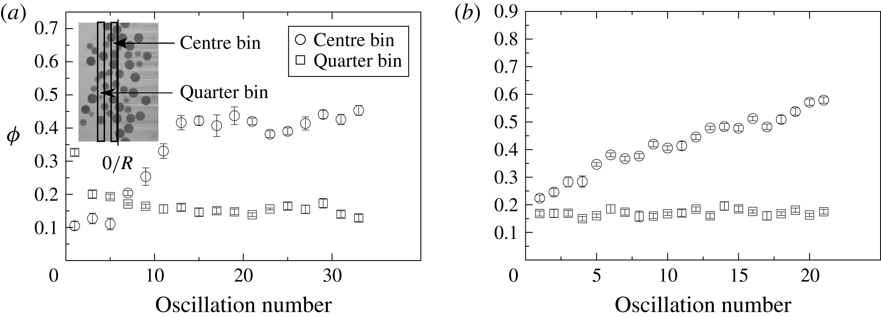
In addition to the dynamics, steady-state results are of interest. Steady state was determined by analysing the average volume fraction. The volume fraction was calculated by averaging over images 10–35 of a given oscillation. When a majority of the bins were within 1.5 standard deviations of the remaining oscillations, an experiment was considered to be at steady state. The determination of steady state did not exhibit a dependence on the number of bins, which was varied from 20 to 50 with intervals of 10. Figure 4(a) shows the evolution of
 ${\it\phi}$
at various bin locations for an experiment with
 ${\it\phi}_{B}=20\,\%$
and
 $R/a=8.21$
. Two different locations are shown, each having a bin width of
 $1/20$
of the diameter. The centre bin began at the centre of the tube. The other bin is centred at a quarter of
 $2R$
and is accordingly termed the quarter bin. The positions of these bins are shown in the inset, which has not been drawn to scale, in figure 4(a). This calculation, performed on the experiments shown in figure 4(a,b), indicates steady state after 16 oscillations and 19 oscillations, respectively. Results shown in § 3.1 were averaged across all the steady-state oscillations, as well as across the different experimental runs (typically 5).
The evolution of the volume fraction is shown for a bin located in the centre (centre bin) and midway between the wall and the centre (quarter bin) for (a)
 $R/a=8.21$
at
 ${\it\phi}_{B}=20\,\%$
and (b)
 $R/a=15.71$
at
 ${\it\phi}_{B}=30\,\%$
.

3. Results and comparisons
3.1. Steady state
The particle volume fraction
 ${\it\phi}$
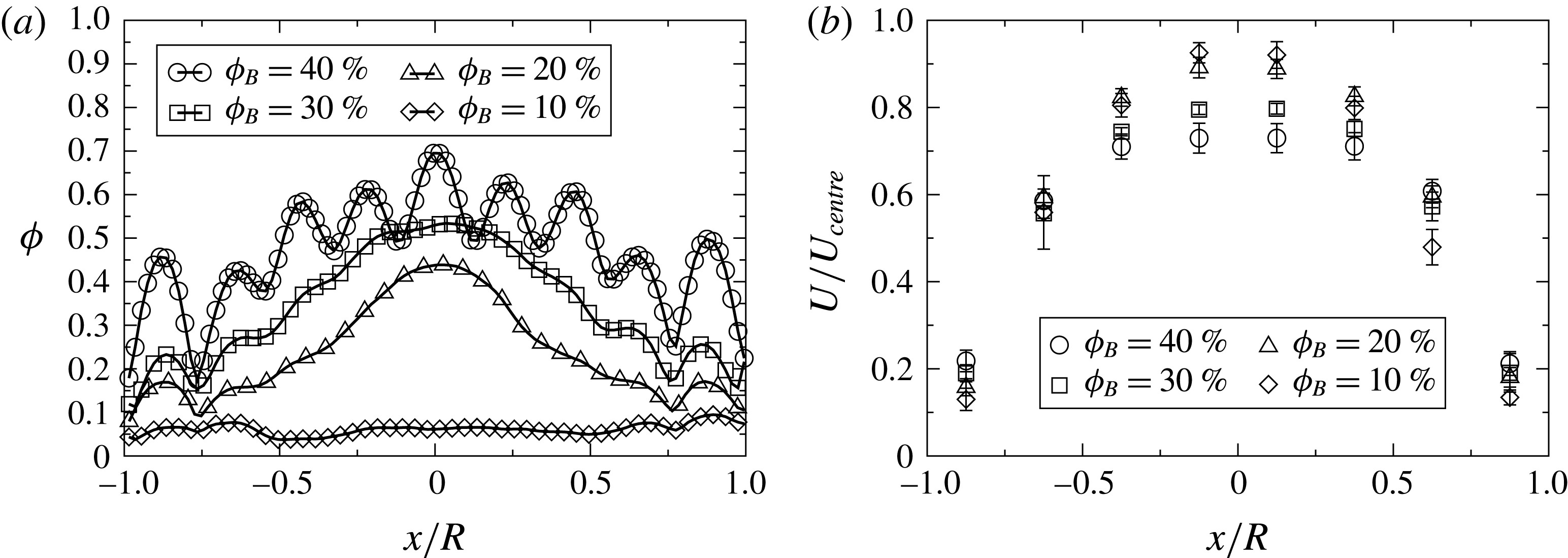
observed at steady state is shown in figure 5(a) for bulk volume fractions of
 ${\it\phi}_{B}=10{-}40\,\%$
at
 $R/a=8.21$
. The amplitude of oscillation was
 ${\it\gamma}=5.4$
(or 44.5 particle radii). The maximum observed volume fraction at steady state decreases with decreasing bulk volume fraction. Distinct particle layers are observed across the tube for
 ${\it\phi}_{B}=40\,\%$
, likely due to the high level of confinement at this concentration and
 $R/a$
. There is no observed migration for
 ${\it\phi}_{B}=10\,\%$
, which will be explored further in § 3.3. Figure 5(b) shows the particle velocity normalised by the centreline velocity
 $U/U_{centre}$
for
 $R/a=8.21$
, where the centreline velocity is that of a Newtonian fluid with a homogeneous viscosity at the same flow rate. A blunting of the velocity profile is consistent with the observed increase in volume fraction at the pipe centre.
Steady-state results ensemble averaged over all the experimental runs at
 $R/a=8.21$
for (a) the volume fraction and (b) particle velocity.

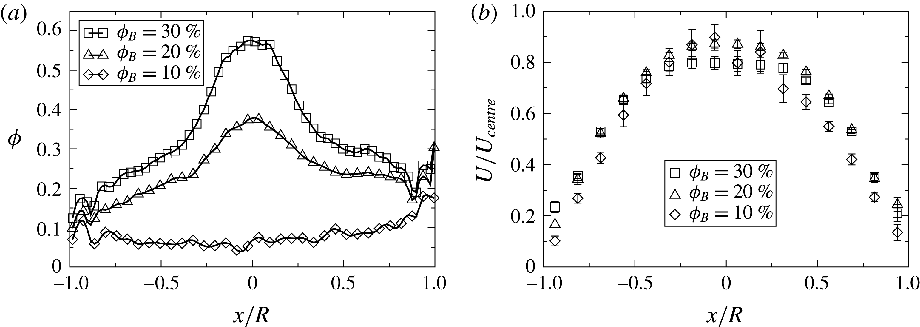
Steady-state results ensemble averaged over all the experimental runs at
 $R/a=15.71$
for (a) the volume fraction and (b) particle velocity.

Observations of the particle volume fraction and particle velocity are shown in figure 6 at bulk volume fractions from 10 % to 30 % for the smaller particle size (
 $R/a=15.71$
). The strain amplitude was
 ${\it\gamma}=5.4$
(or 85.2 particle radii). It is important to note that the image analysis for this geometry resulted in artificially high volume fraction measurements, especially past the centreline of the cylinder opposite the side of the applied laser (
 $x/R=0$
to 1). This was due to the increase in the number of interfaces due to the decrease in particle size. Accordingly, false particles, which were dark imperfections in the original image, artificially increased the volume fraction. This is likely why the maximum volume fraction is higher here than at
 $R/a=8.21$
. Additionally, this issue inhibited experiments at
 ${\it\phi}_{B}=40\,\%$
. Despite complications in the imaging, the trend of decreasing maximum volume fraction with decreasing bulk volume fraction is shown. Again, no migration at
 ${\it\phi}_{B}=10\,\%$
was observed, as will be discussed in § 3.3. The particle velocity profile shows a blunting consistent with the increase in concentration at the centre of the tube.
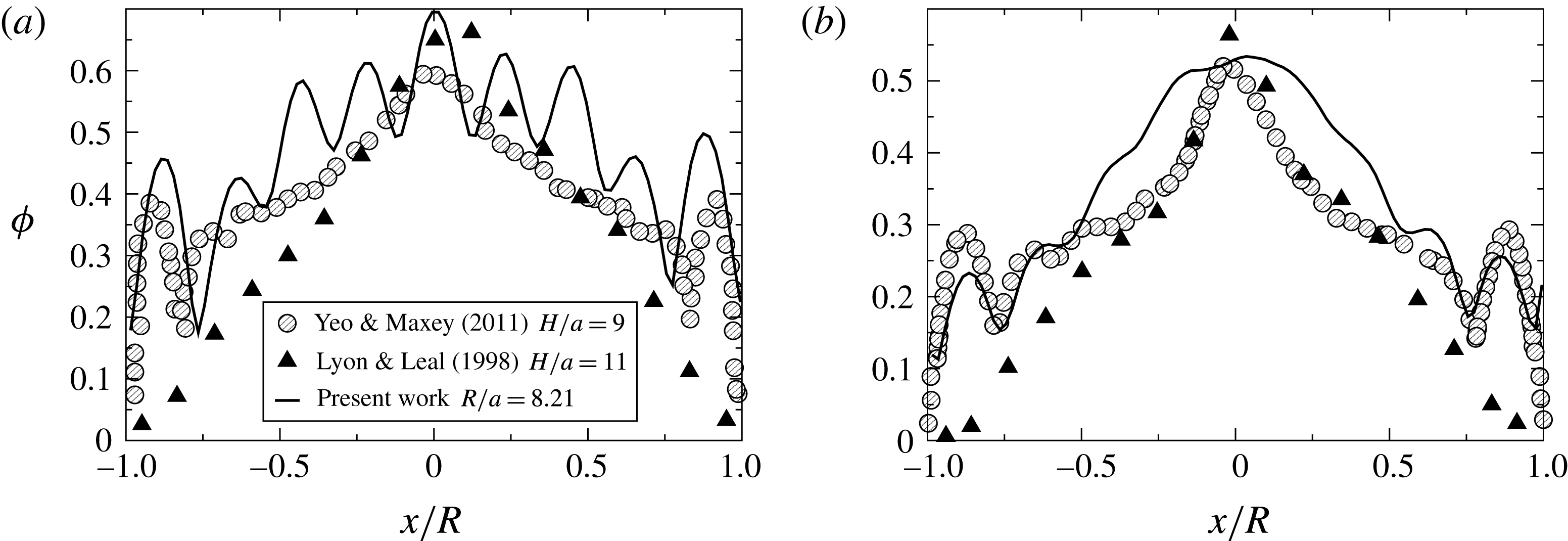
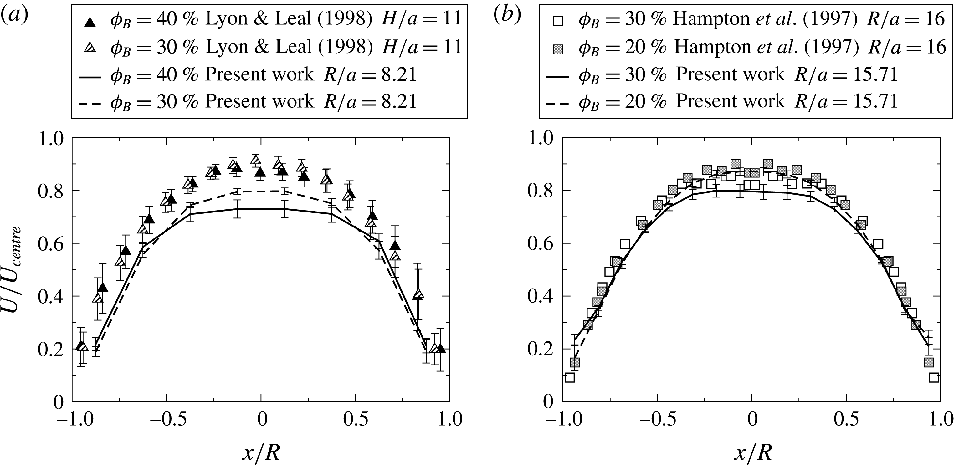
Steady-state results from the present work are compared to previous experimental and numerical work at similar small values of
 $R/a$
for (a)
 ${\it\phi}_{B}=40\,\%$
and (b)
 ${\it\phi}_{B}=30\,\%$
.

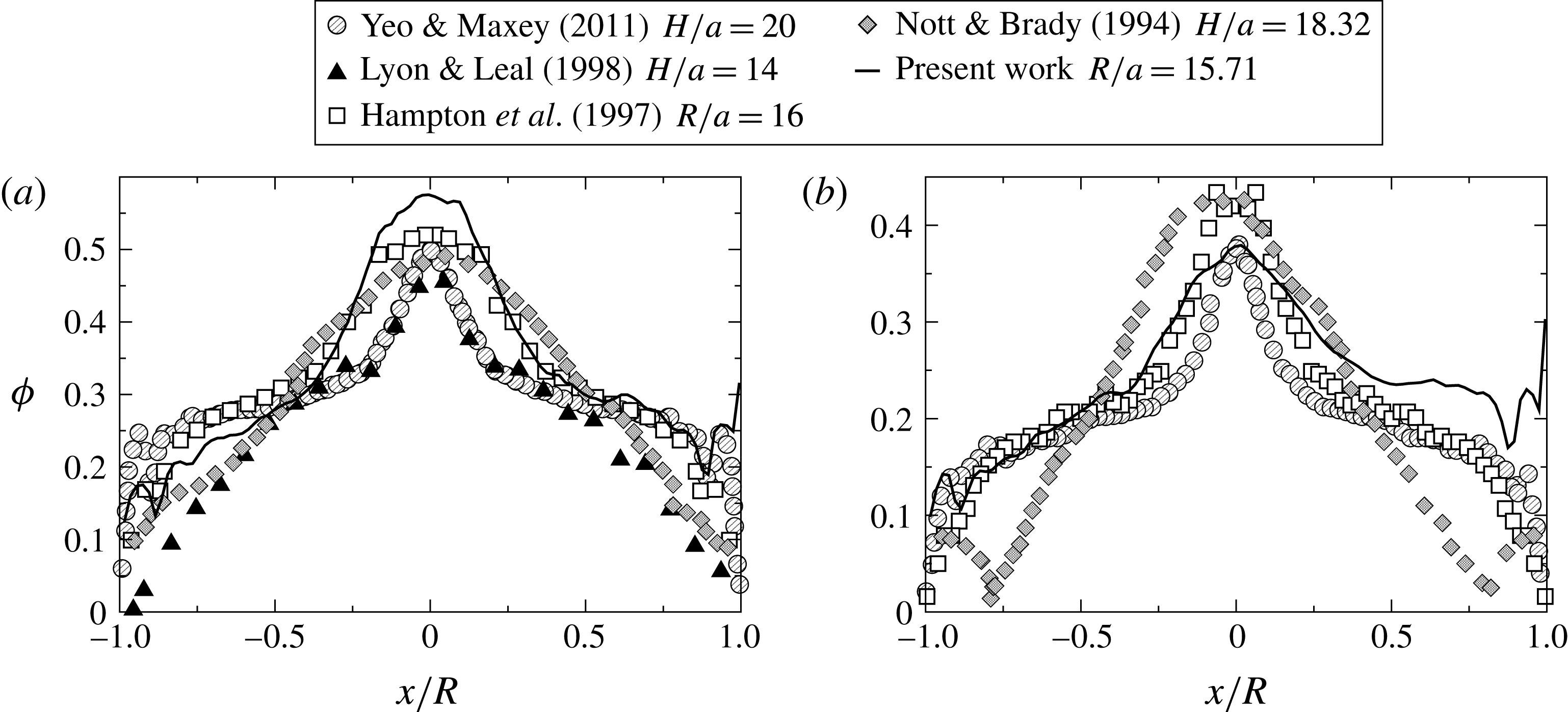
Steady-state results for (a)
 ${\it\phi}_{B}=30\,\%$
and (b)
 ${\it\phi}_{B}=20\,\%$
compared to previous experimental and numerical work at similar larger values of
 $R/a$
.

Figure 7 compares results for the particle volume fraction from the present work to the numerical simulations of Yeo & Maxey (Reference Yeo and Maxey2011) and the experimental measurements of Lyon & Leal (Reference Lyon and Leal1998). Although these previous results are for channel flow, comparisons are made at similar values of
 $H/a$
, where
 $H$
is half the channel height. The experiments reported here and the simulation results both exhibit the formation of layers of particles, though the experiments of Lyon & Leal (Reference Lyon and Leal1998) do not. All of the results shown indicate that the maximum concentration, which occurs at the centre of the tube, is lower than random maximum packing at
 ${\it\phi}_{B}=30\,\%$
. Figure 8 compares the present observations to the experimental results of Hampton et al. (Reference Hampton, Mammoli, Graham, Tetlow and Altobell1997) for pipe flow, as well as to numerical results (Nott & Brady Reference Nott and Brady1994; Yeo & Maxey Reference Yeo and Maxey2011) and the experimental results of Lyon & Leal (Reference Lyon and Leal1998) for channel flow. Again, the results here agree with numerical predictions of the existence of a particle layer near the wall. A decrease in maximum concentration with a decrease in bulk volume fraction was observed for all experimental and numerical results; most noticeably, the concentration at the centre of the tube is only approximately 0.4 for the bulk volume fraction of 20 %.
Steady-state results for the particle velocity compared to previous experimental work for (a)
 $R/a=8.21$
and (b)
 $R/a=15.71$
.

Results for the particle velocity in figure 9(a) show a stronger blunting of the velocity profile for flow in the tube as compared to results for channel flow. Comparisons in figure 9(b) with the results of Hampton et al. (Reference Hampton, Mammoli, Graham, Tetlow and Altobell1997), which were also performed in a circular tube, shows that the present observations are only slightly more blunt. Hence, the results are consistently indicating a significant difference in the steady velocity profile for the different tube shapes.
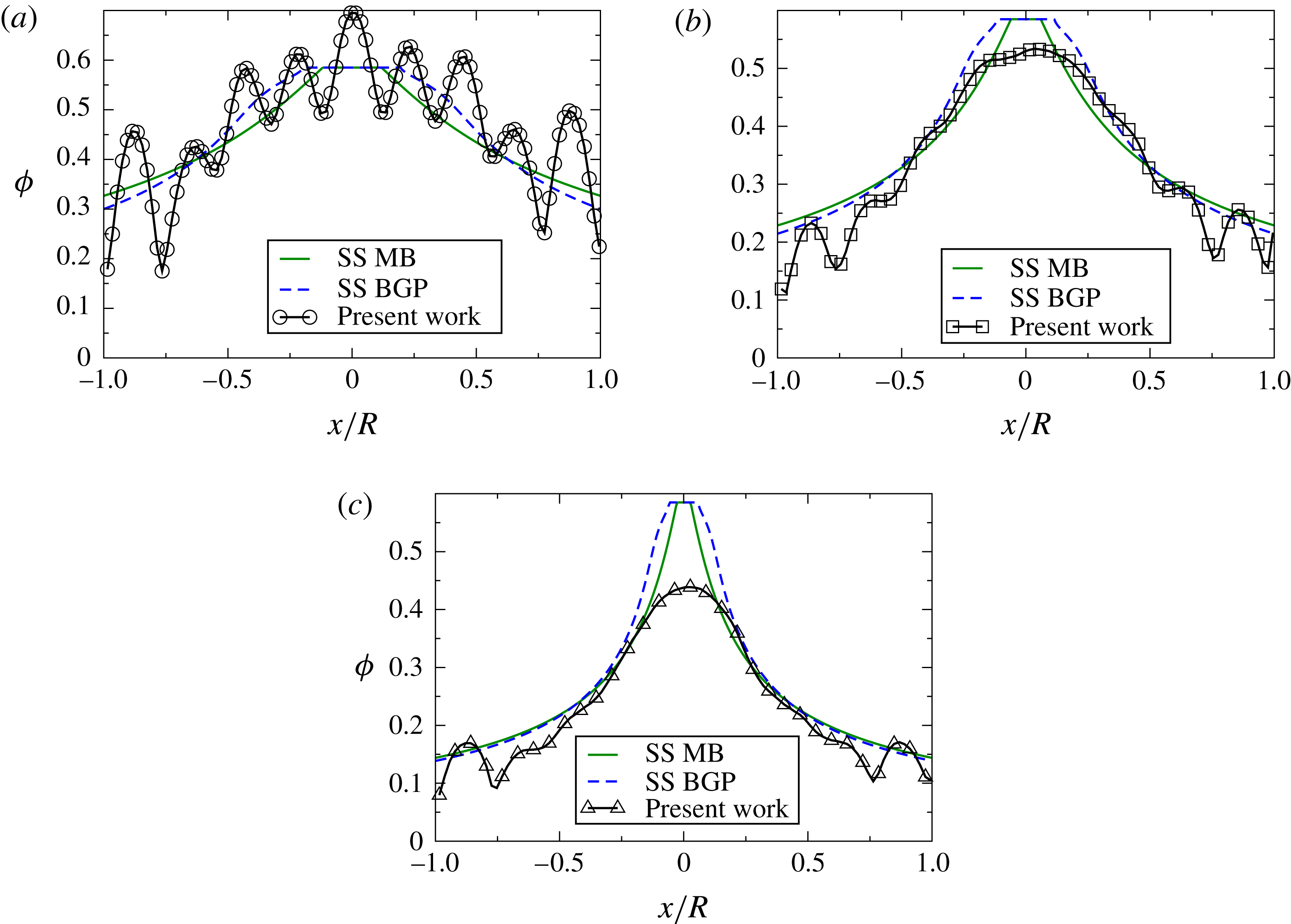
In figures 10 and 11, experiments are compared to the steady-state predictions of the SBM presented in § A.2.1 of the appendix A. This steady-state solution is calculated by requiring a net migration flux of zero and assuming that there is a jammed region at the centre of the pipe. Two slightly different models of the rheologies given by Morris & Boulay (Reference Morris and Boulay1999) and Boyer et al. (Reference Boyer, Guazzelli and Pouliquen2011a
) were used in the numerics. The SBM is a continuum model and thus does not predict the layering observed in the experiments. Nonetheless, taking into account only the average of the magnitude of the concentration profiles, figure 10(a) shows excellent agreement with the SBM predictions for
 ${\it\phi}_{B}=40\,\%$
and
 $R/a=8.21$
. Results in figure 10(b) for
 ${\it\phi}_{B}=30\,\%$
and
 $R/a=8.21$
show a small discrepancy between the numerical predictions and experimental observation for the maximum volume fraction at the centre. The SBM always predicts a centreline concentration equivalent to maximum random packing (
 ${\it\phi}_{m}=.585$
), but the measured concentration did not reach
 ${\it\phi}_{m}$
. This discrepancy increases for
 ${\it\phi}_{B}=20\,\%$
, as seen in figure 10(c).
Steady-state results for
 $R/a=8.21$
compared to the numerical predictions from the steady-state SBM using the Morris & Boulay (Reference Morris and Boulay1999) (MB in legend) and Boyer et al. (Reference Boyer, Guazzelli and Pouliquen2011a
) (BGP in legend) rheology at (a)
 ${\it\phi}=40\,\%$
, (b)
 ${\it\phi}=30\,\%$
, and (c)
 ${\it\phi}=20\,\%$
.

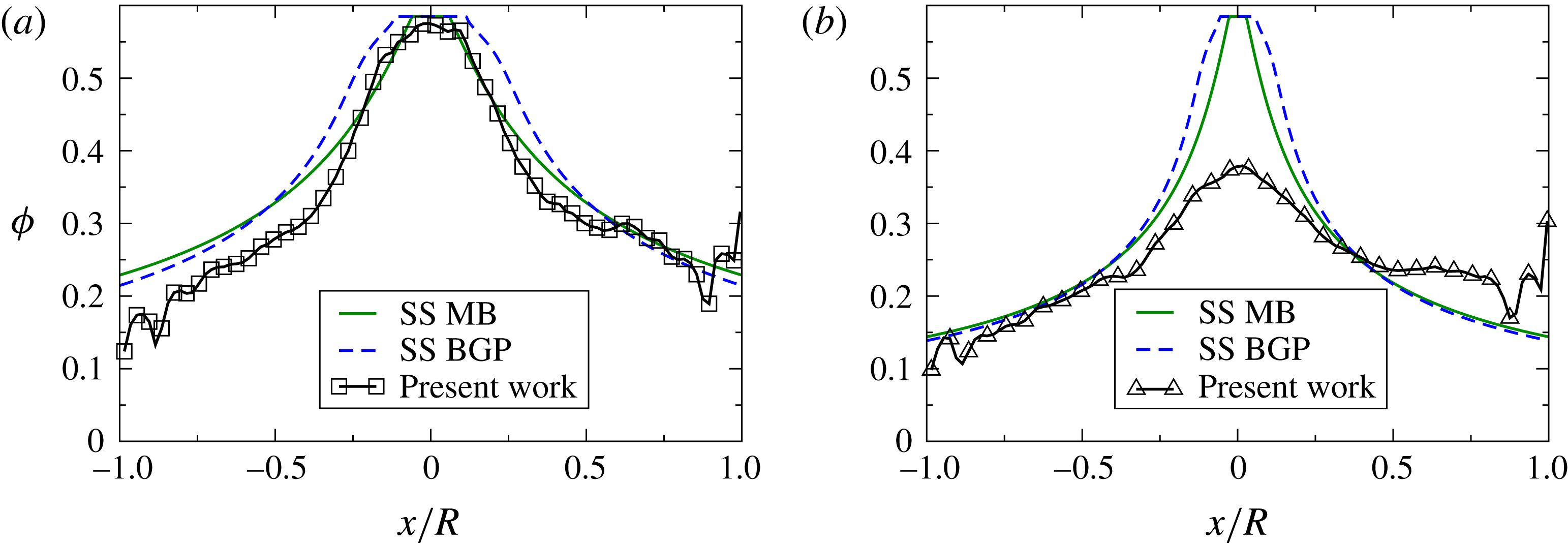
Steady-state results for
 $R/a=15.71$
at (a)
 ${\it\phi}=30\,\%$
and (b)
 ${\it\phi}=20\,\%$
compared to the numerical predictions from the steady-state SBM using the rheology of Morris & Boulay (Reference Morris and Boulay1999) and Boyer et al. (Reference Boyer, Guazzelli and Pouliquen2011a
).

Numerical predictions and experimental observations for the geometry
 $R/a=15.71$
are shown in figure 11. Good agreement is obtained for
 ${\it\phi}_{B}=30\,\%$
(figure 11
a). It should be noted that the experimental observations for
 $R/a=15.71$
are closer to maximum packing
 ${\it\phi}_{m}$
in the centre than those for
 $R/a=8.21$
. This is likely due to the experimental error artificially increasing the observed volume fraction for these particles, as mentioned previously. Results in figure 11(b) for
 ${\it\phi}_{B}=20\,\%$
show a large disagreement between the numerical predictions and the experimental observations in the centre of the pipe. Experimental steady-state data for the particle volume fraction and velocity are given as movies in supplementary materials available online at http://dx.doi.org/10.1017/jfm.2015.645.
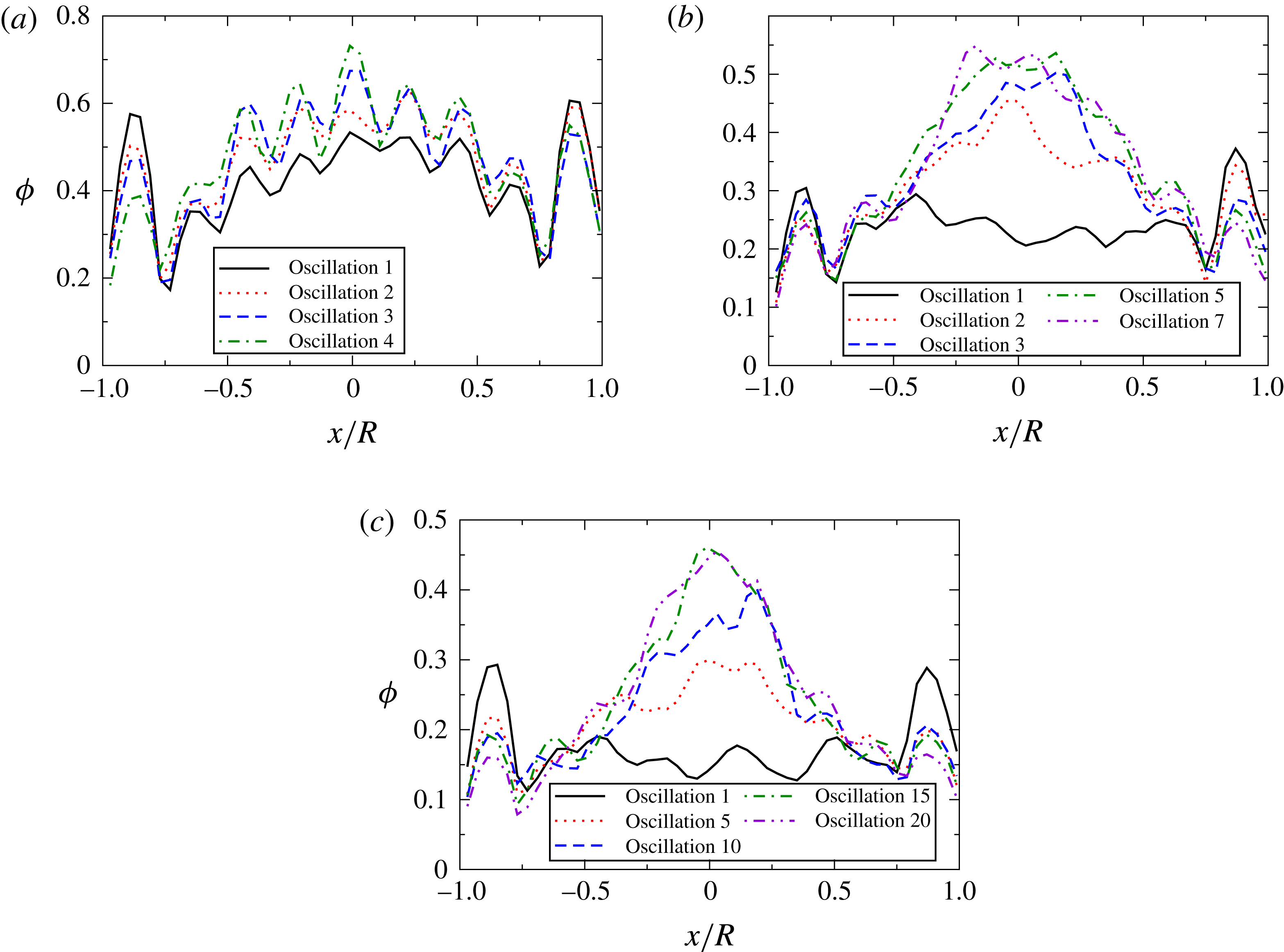
Experimental results for the temporal evolution of the particle volume fraction distributions at
 $R/a=8.21$
for (a)
 ${\it\phi}_{B}=40\,\%$
, (b)
 ${\it\phi}_{B}=30\,\%$
, and (c)
 ${\it\phi}=20\,\%$
.

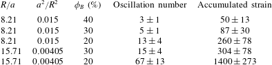
Number of oscillations (or accumulated strain) to steady state. Results are averaged across 3–6 different experiments.

Experimental results for the temporal evolution of the particle volume fraction distributions at
 $R/a=15.71$
for (a)
 ${\it\phi}_{B}=30\,\%$
and (b)
 ${\it\phi}_{B}=20\,\%$
.

3.2. Dynamics
Using the method described in § 2.4, the strain required to achieve the steady profile for the particle concentration has been calculated from the experimental results and reported in table 1. We have reported the average and standard deviation as computed from multiple experimental runs. Within the standard deviation, the accumulated strain to reach steady state is four times larger for the smaller particles, in agreement with the scaling of
 $a^{2}/R^{2}$
that is given by the SBM (see (A 12) of the appendix A). Interestingly, the three data points for
 $R/a=8.21$
indicate that the accumulated strain to reach steady state scales as approximately
 ${\it\phi}_{B}^{-2}$
.
The average
 ${\it\phi}$
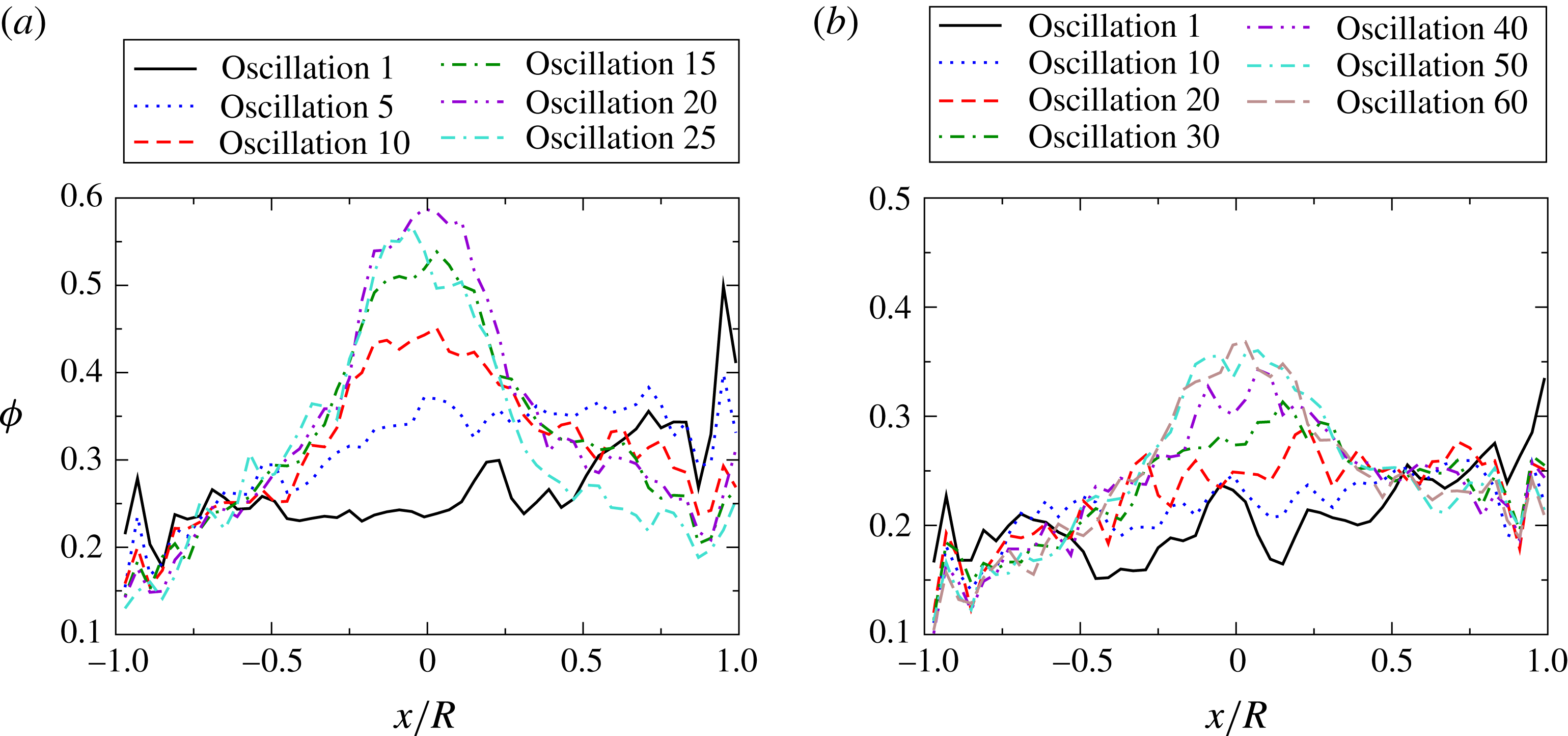
-distributions at different oscillations are shown in figure 12 for
 ${\it\phi}_{B}=20{-}40\,\%$
at
 $R/a=8.21$
and in figure 13 for
 ${\it\phi}_{B}=20\,\%$
and 30 % at
 $R/a=15.71$
. These results are calculated by first dividing an image into
 $50$
bins. Then for a given bin, volume fraction measurements are averaged across images 20–35. A smaller number of images is used as compared to the averaging process for the steady-state results described above, as the system is still dynamic and the objective is to observe the changing distribution. Lastly, results are averaged across the experimental runs for a given
 $R/a$
and
 ${\it\phi}_{B}$
. Particle migration is evidenced by the increase in particle volume fraction at the centre of the cylinder and its decrease at the edges. It is interesting that, despite the decrease in particle volume fraction at the edge, a particle layer is clearly maintained, likely due to the confinement. The dynamics of the migration process also are captured in the online movie 1 where, for every five oscillations, images 1–40 of the oscillation are shown (see supplementary movie 1). The same dynamic behaviour is seen in the averaged velocity profiles which evolve from Poiseuille to plug flows as particles migrate towards the centre of the pipe. Only the concentration profiles are used for quantitative analysis of the dynamics, as the velocity profiles are a less sensitive measure of the dynamics.
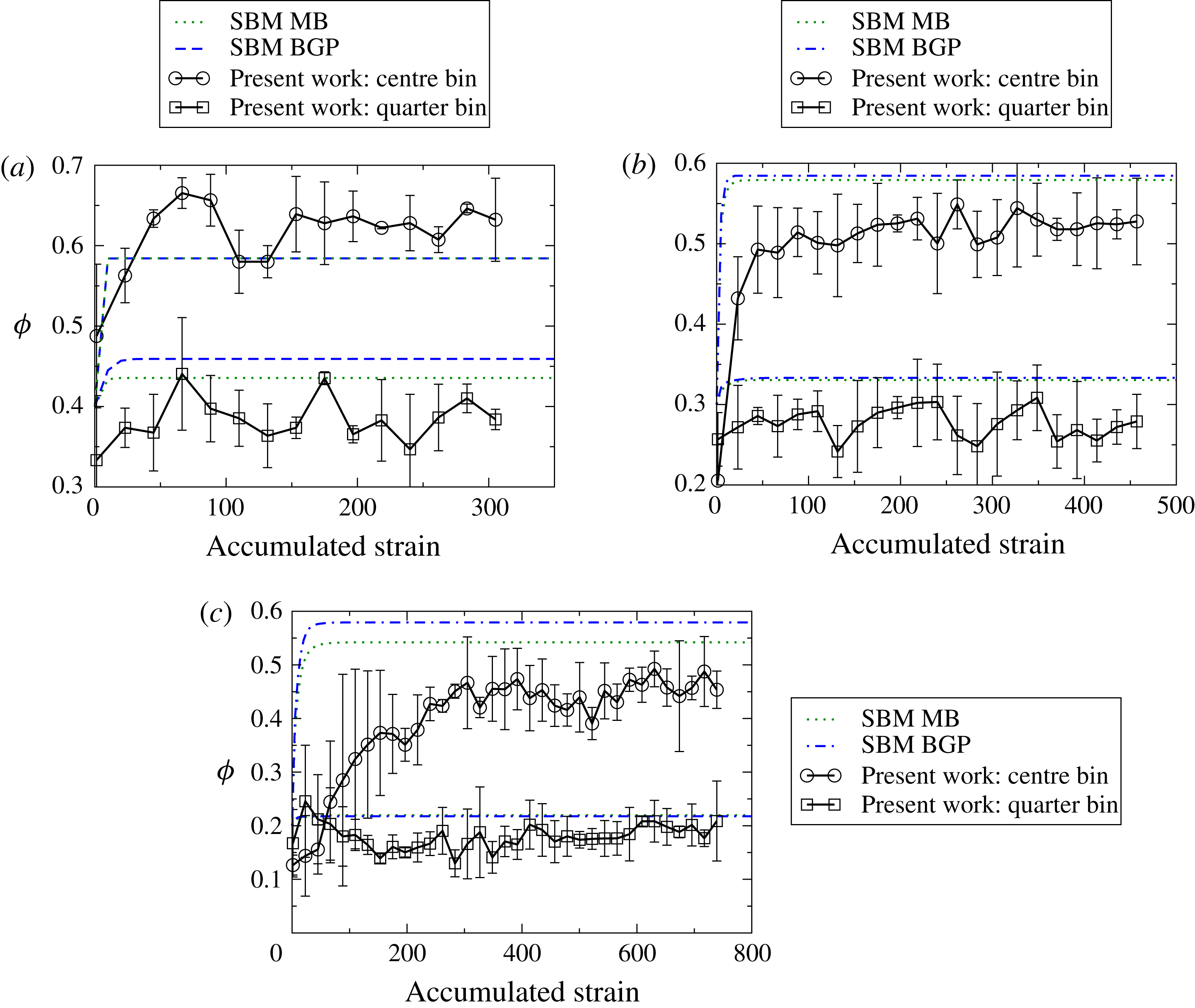
SBM predictions and experimental results for the temporal evolution of the local particle volume fraction at the centre and quarter bins at
 $R/a=8.21$
for (a)
 ${\it\phi}_{B}=40\,\%$
, (b)
 ${\it\phi}_{B}=30\,\%$
, and (c)
 ${\it\phi}=20\,\%$
.

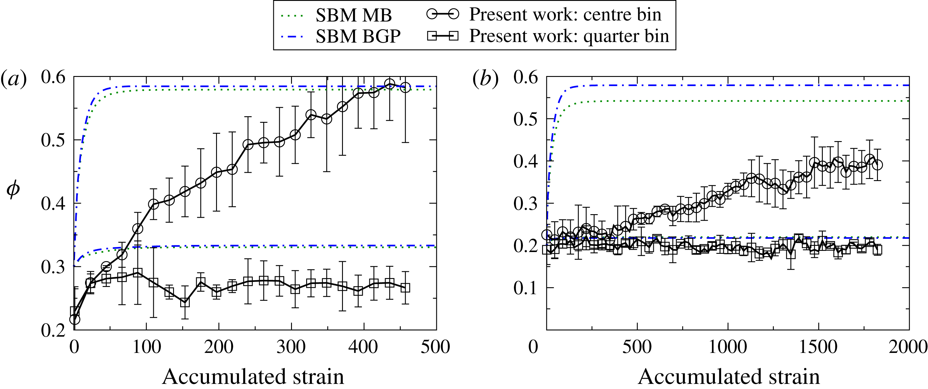
SBM predictions and experimental results for the temporal evolution of the local particle volume fraction at the centre and quarter bins at
 $R/a=15.71$
for (a)
 ${\it\phi}_{B}=30\,\%$
and (b)
 ${\it\phi}_{B}=20\,\%$
.

To examine further the temporal evolution of
 ${\it\phi}$
, dynamic experimental results are plotted in figures 14 and 15. The data are averaged across different experimental runs for each given bin location using images 20–35. The centre bin corresponds to
 $1/20$
th of the cylinder width, beginning at the centre of the tube, and the quarter bin corresponds to
 $1/20$
th of the tube width centred at one quarter of the total tube width. Dynamic predictions from the SBM, as described in § A.2.2 of the appendix A, are also plotted on these figures using the same centre and quarter bins. Note that the predictions using the rheology of Boyer et al. (Reference Boyer, Guazzelli and Pouliquen2011a
) always attains a concentration of
 ${\it\phi}_{m}$
at the centre bin when steady state is reached, while the predictions using the rheology of Morris & Boulay (Reference Morris and Boulay1999) do not. For the latter rheology, the extent of the central plug is smaller than the bin size, and hence the value is always a little lower than
 ${\it\phi}_{m}$
, whereas the central plug is larger when using the rheology of Boyer et al. (Reference Boyer, Guazzelli and Pouliquen2011a
) as can be seen in figures 10 and 11.
For the largest bulk volume fraction of
 ${\it\phi}_{B}=40\,\%$
at
 $R/a=8.21$
(figure 14), the experiments rapidly reach a high concentration at the centre of the tube, as predicted by the model. For the smaller bulk volume fraction of
 ${\it\phi}_{B}=30\,\%$
, the experimental observations show a slower evolution to steady state than predicted and, as noted previously, the experiments never reach the concentration predicted by the models for the centre bin. The discrepancy between the observed and predicted rates of migration increases at the lower
 ${\it\phi}_{B}$
of 20 %. The disagreement between the dynamic numerical predictions and experimental observations is even greater for
 $R/a=15.71$
, as seen in figure 15.
The data for the dynamics of the particle volume fraction distribution are included online; see supplementary materials. Experimental measurements of the evolution of the volume fraction for the centre and quarter bins are also available.
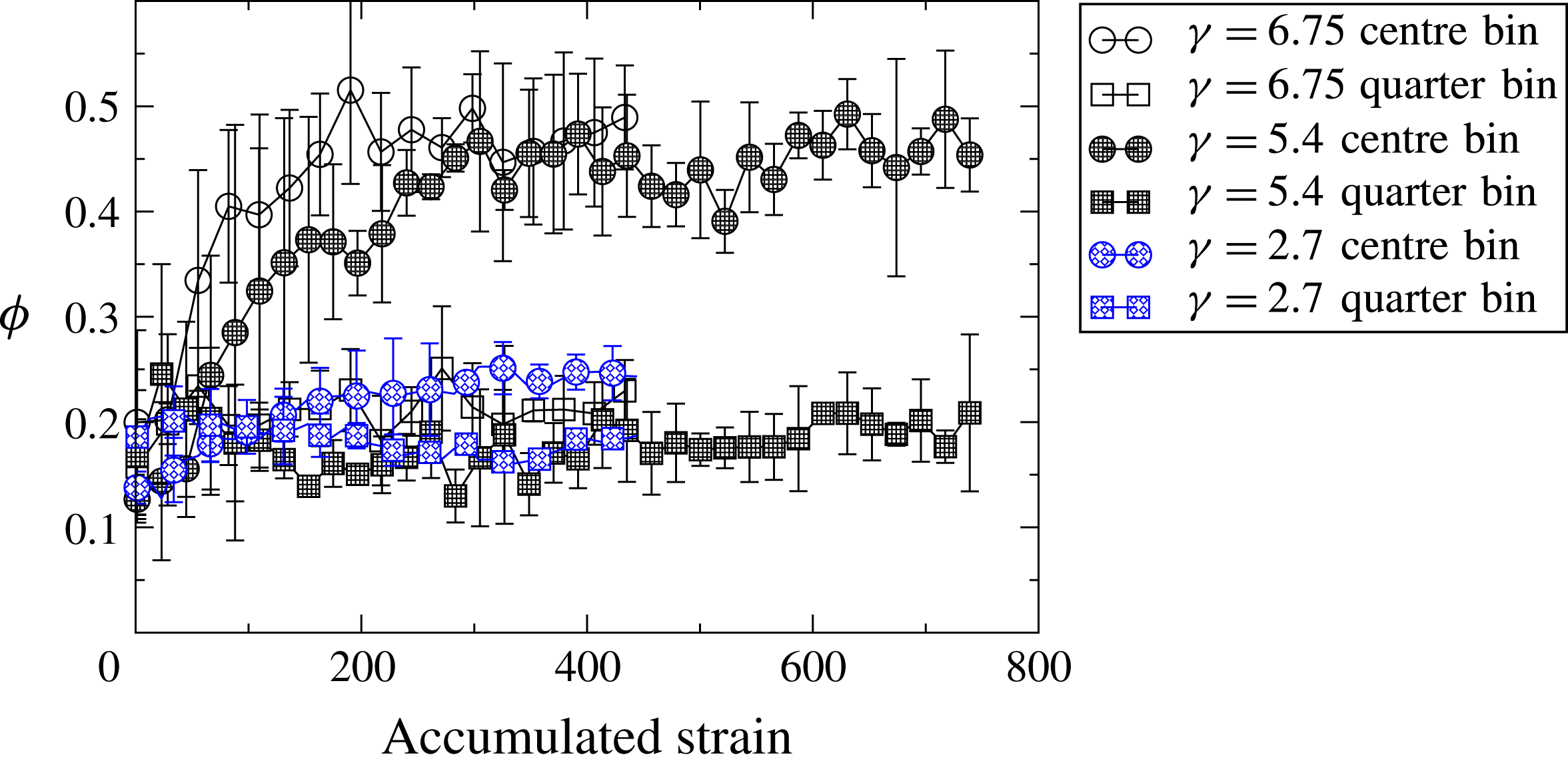
Temporal evolution of the local particle volume fraction at the centre (circle) and quarter (square) bins for
 $R/a=8.21$
at
 ${\it\phi}_{B}=20\,\%$
for
 ${\it\gamma}=2.7,5.4,$
and
 $6.75$
.

3.3. Migration dependence on concentration and strain
To test the effect of strain amplitude on the migration process, the amplitude was increased to
 ${\it\gamma}=6.75$
for
 $R/a=8.21$
and
 ${\it\phi}_{B}=20\,\%$
. Experimental measurements were averaged in the same way as in figures 14 and 15 and as described in § 3.2. Figure 16 shows that, within the experimental error, the volume fraction profile reaches the same steady state at approximately the same accumulated strain. Testing with a much larger amplitude
 ${\it\gamma}$
would have been desirable, but this would require a much longer tube to safely avoid end effects. Performing experiments at
 ${\it\phi}_{B}=20\,\%$
for a smaller strain amplitude of
 ${\it\gamma}=2.7$
generates little to no migration, as also plotted in figure 16.
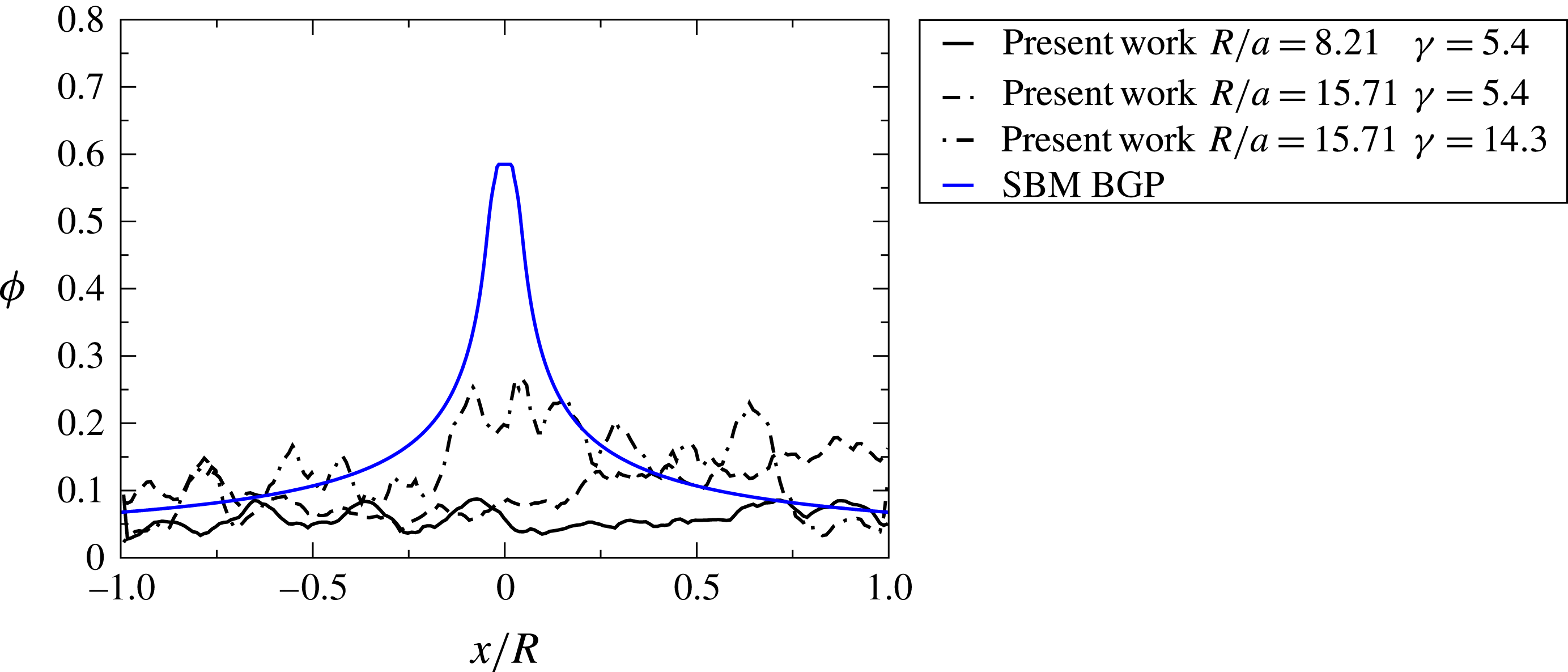
No migration was observed at
 ${\it\phi}_{B}=10\,\%$
for either particle size (
 $R/a=8.21$
and
 $R/a=15.71$
), as seen in figure 17. For
 $R/a=8.21$
, experiments were stopped after 50 oscillations, or an accumulated strain of 1085 at
 ${\it\gamma}=5.4$
; for
 $R/a=15.71$
, experiments were stopped after 30 oscillations, or an accumulated strain of 630. To further test the lack of observable migration, the amplitude was increased to 14.32 (or 225 particle radii) for
 $R/a=15.71$
at
 ${\it\phi}_{B}=10\,\%$
. After stopping the experiments after 20 oscillations (or an accumulated strain of 945), large fluctuations in the volume fraction profile can be seen, but no net migration is detected.
The experimentally observed volume fraction distribution at the beginning of the final oscillation for different
 $R/a$
and
 ${\it\gamma}$
at
 ${\it\phi}_{B}=10\,\%$
. No observable migration is exhibited in the experimental results, but the SBM using Boyer et al. (Reference Boyer, Guazzelli and Pouliquen2011a
) rheology (solid blue line) predicts migration.

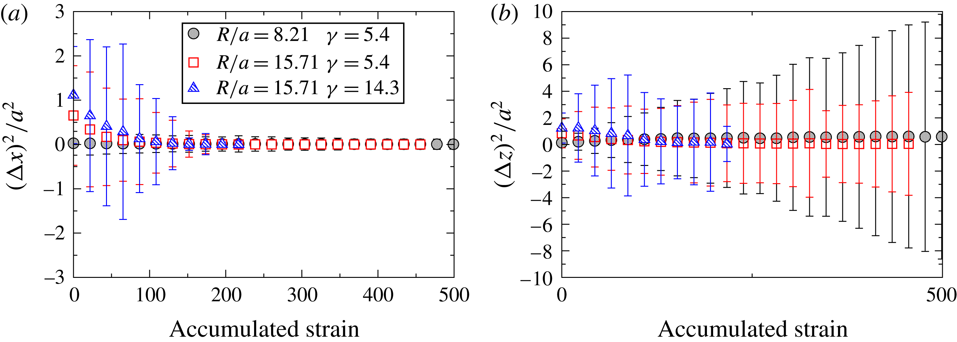
Mean-square displacement of the particles (a) transverse to the flow and (b) along the flow for different
 $R/a$
,
 ${\it\gamma}$
, and
 ${\it\phi}_{B}=10\,\%$
.

To investigate the absence of observed migration at
 ${\it\phi}_{B}=10\,\%$
, the mean-square displacement of the particles was measured and ensemble averaged across particles and experimental runs. The results are plotted in figure 18 and there is some limited evidence of a non-zero component of the displacements in directions transverse to the flow at small accumulated strains. However, even for those points, the mean-square displacements, if non-zero, are too small to measure with any accuracy and the particle motion can be considered as quasi reversible. Additional, direct evidence of the reversible particle motions can be seen in the online movie 2, where the suspension is shown stroboscopically across all oscillations (see supplementary movie 2). In contrast, the online movie 3 at
 ${\it\phi}_{B}=20\,\%$
displays strong irreversibility (see supplementary movie 3).
4. Discussion and conclusions
The spatial and temporal dependence of the particle volume fraction and velocity for suspensions of neutrally-buoyant spheres in oscillatory pipe flow was experimentally studied using direct imaging techniques. The bulk volume fraction
 ${\it\phi}_{B}$
was varied from 10 % to 40 % and the pipe to sphere radius was set at either
 $R/a=8.21$
or
 $R/a=15.71$
. Not only the final distributions, but also the dynamics of the shear-induced migration, were analysed and compared to previous work and to predictions of the SBM using two different rheological models.
The measurements at steady state of the volume fraction profiles and previous results from experiments and discrete-particle simulations are consistent when compared for similar values of concentration of 20 % or higher and tube-to-particle size ratio. This includes the observation of particle layering (see figure 7) which has been predicted in simulations of tube flow and seen in some experiments on simple shearing flows (Deshpande & Shapley Reference Deshpande and Shapley2010; Blanc et al.
Reference Blanc, Lemaire, Meunier and Peters2013), though not in tube flow. This particle layering is likely due to the strong confinement of the particles, or low ratio of
 $R/a$
; note that the layering is not as prominent for the data shown in figure 8, where the ratio of
 $R/a$
is nearly twice as large. The data comparisons of the steady profiles shown in figures 7 and 8 also consistently indicate that the volume fraction at the centre of the geometry drops as
 ${\it\phi}_{B}$
decreases.
Comparing the measurements with the steady-state calculations of the SBM (figures 10 and 11) demonstrate that the continuum calculation is unable, of course, to predict the particle layers. However, the model does roughly agree with the averaged data at large
 ${\it\phi}_{B}$
. At smaller values of
 ${\it\phi}_{B}$
, the SBM fails to predict that the steady concentration at the centre of the pipe falls below that of maximum packing, in contradiction to the observations.
The dynamics of the shear-induced migration process were also measured and reported as part of this work. The results concerning the dynamics can be compared only to the solutions given by the SBM, since data from previous experimental or discrete-particle numerical work are not readily available. Qualitatively, the SBM supports the experimental observations that the total strain to attain the steady profile is consistent with general scalings of
 $a^{2}/R^{2}$
and decreases with
 ${\it\phi}_{B}$
. However, the predictions reach steady state significantly faster than the experiments, save for the largest
 ${\it\phi}_{B}$
of 40 % that was studied here.
Importantly, we note that oscillating the flow with sufficiently large amplitudes does not change the steady-state results as compared to the alternative of driving the suspension flow with a steady pressure gradient through a very long tube. Firstly, the present oscillatory-flow data compare well with the steady-flow observations found in the literature, as argued above. Secondly, figure 16 shows that the steady results are equivalent for
 ${\it\gamma}\gtrsim 5.4$
, within the experimental error. This was also observed in previous oscillatory experiments and was suggested in modelling efforts (Butler et al.
Reference Butler, Majors and Bonnecaze1999; Morris Reference Morris2001; Yapici, Powell & Phillips Reference Yapici, Powell and Phillips2009). The question of whether the dependence of the dynamics on the strain, or time, in oscillatory flows are equivalent to those in steady flows is more difficult to assess, owing in part to the lack of previous dynamic experiments with which to compare. However, the direct test shown in figure 16 suggests that the dynamics is the same for large strain amplitudes (
 ${\it\gamma}\gtrsim 5.4$
), even at the relatively low concentration of
 ${\it\phi}_{B}=20\,\%$
.
Figure 16 also indicates that little migration, if any, occurs for sufficiently small strain amplitudes, at least over an accumulated strain of 450. Also, no migration was observed for
 ${\it\phi}_{B}=10\,\%$
as illustrated in figure 17, even for strain amplitudes as large as 14.3. Two possibilities to explain this latter result are feasible: no migration takes place at such low volume fractions even for steady flows, or the strain amplitude is too small to generate migration for
 ${\it\phi}_{B}=10\,\%$
. Regarding the former possibility, migration may simply not occur because normal stresses, which are mostly driven by contact forces, are too low or even non-existent for
 ${\it\phi}_{B}\lesssim 10\,\%$
. Previous experiments on steady flows through a pipe (Hampton et al.
Reference Hampton, Mammoli, Graham, Tetlow and Altobell1997) reported an absence of migration, but experiments in a channel by Koh & Leal (Reference Koh and Leal1994) and Stokesian dynamics simulations (Nott & Brady Reference Nott and Brady1994) did exhibit migration.
Assuming that migration should occur under steady flow for
 ${\it\phi}_{B}=10\,\%$
, the present experiments are evidence of an amplitude and a concentration threshold requirement for migration. The existence of an amplitude threshold is in agreement with previous work on pressure-driven flows (Butler et al.
Reference Butler, Majors and Bonnecaze1999; Guasto, Ross & Gollub Reference Guasto, Ross and Gollub2010) and is consistent with experiments on the reversibility of particle motion in oscillatory shear flows (Pine et al.
Reference Pine, Gollub, Brady and Leshansky2005). The threshold strain amplitude for the onset of irreversibility as a function of volume fraction (see figure 3 of Pine et al.
Reference Pine, Gollub, Brady and Leshansky2005) increases dramatically below
 ${\it\phi}_{B}=10\,\%$
and even seems to diverge. Note that the situation is far more complex for non-uniform strain as the transition is pushed to larger wall strain amplitudes (see figure 4 of Guasto et al.
Reference Guasto, Ross and Gollub2010) and occurs simultaneously across the channel. Consequently the lack of migration observed in the present experiments at
 ${\it\phi}_{B}=10\,\%$
may not be surprising.
The detailed experimental results provided by this work represent an opportunity for improving the continuum modelling of shear-induced migration (in particular the SBM) through direct comparisons. Two issues of concern are the prediction of the centreline concentration and the comparison of the rates of migration. To aid in resolving these issues in future studies, several points should be noted. Firstly, the two rheological laws used here are strictly valid for large
 ${\it\phi}_{B}$
and have been extrapolated for
 ${\it\phi}_{B}\leqslant 40\,\%$
. The rheological law of Morris & Boulay (Reference Morris and Boulay1999) was meant to match experimental results of migration at large
 ${\it\phi}_{B}$
and that of Boyer et al. (Reference Boyer, Guazzelli and Pouliquen2011a
) was obtained from measurements for
 ${\it\phi}_{B}\gtrsim 40\,\%$
. These rheologies may have to be altered for lower concentrations. Secondly, the phenomenological form for the normal stress of the particle phase was chosen for simplicity to have a similar concentration dependence in all directions, as proposed by Morris & Boulay (Reference Morris and Boulay1999). However, there may be some slow variation in the different directions which may need to be included in the model (Dbouk, Lobry & Lemaire Reference Dbouk, Lobry and Lemaire2013; Gallier et al.
Reference Gallier, Lemaire, Peters and Lobry2014). Finally, normal stresses near the pipe walls, where layering occurs due to confinement effects, may differ from those in the bulk middle region of the pipe as found in the force coupling simulations of Yeo & Maxey (Reference Yeo and Maxey2011) and in the fictitious domain simulations of Gallier (Reference Gallier2014). This is not captured by the present SBM which uses a rheology that is homogeneous across the pipe.
Applying a non-local correction to the SBM, regardless of the choice of the rheological model, can lower the concentration predicted at the centreline, but this option introduces additional issues. Non-local corrections have been introduced to account for particles sampling neighbouring flow regions over their own size scale or over the scale characteristic of interactions with near neighbours. Different approaches have been used (see e.g. Nott & Brady Reference Nott and Brady1994; Mills & Snabre Reference Mills and Snabre1995; Morris & Boulay Reference Morris and Boulay1999; Miller & Morris Reference Miller and Morris2006). In Nott & Brady (Reference Nott and Brady1994) the non-local stress is written as a function of the fluctuating motions of the particles, which leads to an additional field variable, the suspension temperature. In Mills & Snabre (Reference Mills and Snabre1995), the non-local stress is attributed to the effect of large-scale particle clusters and thus is integrated over the length scale of these large structures. In Morris & Boulay (Reference Morris and Boulay1999) and Miller & Morris (Reference Miller and Morris2006), the non-local stress corresponds to a spatial averaging of the shear rate in the constitutive law for the normal stresses. As demonstrated in § A.2.3 in appendix A, this latter approach leads to a significant decrease in maximum concentration at the centre of the pipe. However, the predicted profile for the volume fraction distribution is faulty at the centre of the pipe and the non-local stress modelling relies on ad hoc parameters.
Another alternative is to use a microstructural model of the rheology (Goddard Reference Goddard2006; Stickel, Phillips & Powell Reference Stickel, Phillips and Powell2006) for the inputs to the SBM. For steady shearing flows, there is little advantage to using such models over correlations such as those used in this work. However, unsteady flows exhibit a variety of phenomena that cannot be addressed by models derived from the steady shear rheology, such as the transient stresses exhibited during a shear reversal (Gadala-Maria & Acrivos Reference Gadala-Maria and Acrivos1980; Kolli, Pollauf & Gadala-Maria Reference Kolli, Pollauf and Gadala-Maria2002). Only simulations (Bricker & Butler Reference Bricker and Butler2007) or microstructural models (Stickel, Phillips & Powell Reference Stickel, Phillips and Powell2007) can predict those transient stresses. Yapici et al. (Reference Yapici, Powell and Phillips2009) applied the microstructural model of Stickel et al. (Reference Stickel, Phillips and Powell2006) to the calculation of migration in a pipe and, consistent with the findings of Butler et al. (Reference Butler, Majors and Bonnecaze1999) and those shown here, found that the migration profiles return toward those of steady flows for sufficiently large amplitudes. The use of an accurate microstructural model might predict a better estimate of the accumulated strain required to attain the fully developed and steady concentration profile, but at the cost of significant increases in the complexity of the model.
The present experimental data can be used as a benchmark not only for rheological models in the SBM, but also for particle interaction models in discrete-particle simulations. The experimental data and the Matlab codes used to produce the numerical solutions of the SBM are available as supplementary material.
Acknowledgements
This work is supported by the National Science Foundation under grant no. (0968313). It is also undertaken under the auspices of ANR project ‘Dense Particulate Systems’ (ANR-13-IS09-0005-01), ‘Laboratoire d’Excellence Mécanique et Complexité’ (ANR-11-LABX-0092), and the ‘Initiative d’Excellence’ A
 $^{\ast }$
MIDEX (ANR-11-IDEX-0001-02). B.S. acknowledges support from a Chateaubriand Fellowship provided by the Embassy of France. Additionally we would like to thank J. F. Morris for discussions.
Supplementary data
Supplementary data are available at http://dx.doi.org/10.1017/jfm.2015.645.
Appendix A. The suspension balance model (SBM)
A.1. Two-phase modelling
The SBM is derived from a two-phase modelling of the particulate suspension written at low Reynolds number (Nott & Brady Reference Nott and Brady1994; Morris & Boulay Reference Morris and Boulay1999; Lhuillier Reference Lhuillier2009; Nott et al. Reference Nott, Guazzelli and Pouliquen2011). The equations of motion are usually written for the suspension mixture and the particulate phase.
The balance equations for the suspension are
 $$\begin{eqnarray}\displaystyle & \displaystyle \boldsymbol{{\rm\nabla}}\boldsymbol{\cdot }\boldsymbol{u}=0, & \displaystyle\end{eqnarray}$$
 $$\begin{eqnarray}\displaystyle & \displaystyle \boldsymbol{{\rm\nabla}}\boldsymbol{\cdot }{\it\bf\Sigma}+{\it\rho}\boldsymbol{g}=0, & \displaystyle\end{eqnarray}$$
 $\boldsymbol{u}={\it\phi}\boldsymbol{u}^{\boldsymbol{p}}+(1-{\it\phi})\boldsymbol{u}^{\boldsymbol{f}}$
is the volume average velocity of the suspension (
 $\boldsymbol{u}^{\boldsymbol{p}}$
and
 $\boldsymbol{u}^{\boldsymbol{f}}$
are the local mean particle and fluid velocities, respectively),
 ${\it\rho}={\it\phi}{\it\rho}_{p}+(1-{\it\phi}){\it\rho}_{f}$
is the density of the suspension (
 ${\it\rho}_{p}$
and
 ${\it\rho}_{f}$
are the particle and fluid density, respectively) and
 ${\it\bf\Sigma}$
is the bulk average suspension stress.
The particle mass conservation equation yields
 $$\begin{eqnarray}\frac{\partial {\it\phi}}{\partial t}+\boldsymbol{{\rm\nabla}}\boldsymbol{\cdot }({\it\phi}\boldsymbol{u}^{\boldsymbol{p}})=0,\end{eqnarray}$$
which, using the incompressibility of the suspension (A 1), can be rewritten as
 $$\begin{eqnarray}\frac{\partial {\it\phi}}{\partial t}+\boldsymbol{u}\boldsymbol{\cdot }\boldsymbol{{\rm\nabla}}{\it\phi}=-\boldsymbol{{\rm\nabla}}\boldsymbol{\cdot }{\it\phi}(\boldsymbol{u}^{\boldsymbol{p}}-\boldsymbol{u}),\end{eqnarray}$$
to exhibit the migration flux
 ${\it\phi}(\boldsymbol{u}^{\boldsymbol{p}}-\boldsymbol{u})$
. The balance equation for the momentum of the particle phase is
 $$\begin{eqnarray}\boldsymbol{{\rm\nabla}}\boldsymbol{\cdot }{\it\bf\Sigma}^{\boldsymbol{p}}+n\langle \boldsymbol{F}^{\boldsymbol{H}}\rangle +{\it\phi}({\it\rho}_{p}-{\it\rho}_{f})\boldsymbol{g}=0,\end{eqnarray}$$
where the particle-phase stress
 ${\it\bf\Sigma}^{\boldsymbol{p}}$
comprises contact (or interparticle force) contributions as well as hydrodynamic contributions coming from the non-drag part of the interphase force (Lhuillier Reference Lhuillier2009; Nott et al.
Reference Nott, Guazzelli and Pouliquen2011). The hydrodynamic force
 $n\langle \boldsymbol{F}^{\boldsymbol{H}}\rangle$
is approximated by the drag force, which is proportional to the relative velocity between the phases and is given by
 $$\begin{eqnarray}\boldsymbol{F}^{\boldsymbol{D}}=-\frac{9{\it\eta}_{f}}{2a^{2}}\frac{{\it\phi}}{f({\it\phi})}(\boldsymbol{u}^{\boldsymbol{p}}-\boldsymbol{u})\end{eqnarray}$$
for spherical particles of radius
 $a$
; the viscosity of the pure fluid is
 ${\it\eta}_{f}z$
. The empirical hindered settling function proposed by Richardson & Zaki (Reference Richardson and Zaki1954),
 $$\begin{eqnarray}f({\it\phi})=(1-{\it\phi})^{n},\end{eqnarray}$$
is used with an exponent of
 $n\simeq 5$
for low Reynolds numbers.
For neutrally buoyant particles (
 ${\it\rho}={\it\rho}_{p}={\it\rho}_{f}$
), the momentum (A 5) together with the expression for the drag (A 6) provides the migration flux
 $$\begin{eqnarray}{\it\phi}(\boldsymbol{u}^{\boldsymbol{p}}-\boldsymbol{u})=\frac{2a^{2}f({\it\phi})}{9{\it\eta}_{f}}\boldsymbol{{\rm\nabla}}\boldsymbol{\cdot }{\it\bf\Sigma}^{\boldsymbol{p}}.\end{eqnarray}$$
Only the diagonal components of the particle-phase stress tensor
 ${\it\bf\Sigma}^{\boldsymbol{p}}$
, i.e. the normal stress tensor of the particle phase, generate a cross-stream migration flux. It is necessary to assume a phenomenological form which, for simplicity, can be chosen to have a viscous scaling and a similar
 ${\it\phi}$
-dependence in all directions (Morris & Boulay Reference Morris and Boulay1999):
 $$\begin{eqnarray}-{\it\eta}_{f}\dot{{\it\gamma}}\hat{{\it\eta}}_{n}({\it\phi})\left(\begin{array}{@{}ccc@{}}{\it\lambda}_{1} & 0 & 0\\ 0 & {\it\lambda}_{2} & 0\\ 0 & 0 & {\it\lambda}_{3}\end{array}\right),\end{eqnarray}$$
where
 $\dot{{\it\gamma}}$
is the shear rate, the
 ${\it\lambda}_{i}$
(
 $i=1,2,3$
) are scalar parameters which are independent of
 ${\it\phi}$
and
 $\hat{{\it\eta}}_{n}({\it\phi})$
is a dimensionless ‘normal viscosity’ that can be defined as
 $\hat{{\it\eta}}_{n}({\it\phi})=-{\it\Sigma}_{11}^{p}/{\it\eta}_{f}\dot{{\it\gamma}}$
to give
 ${\it\lambda}_{1}=1$
.
A.2. The SBM for pipe flow
For the axisymmetric pipe geometry, (A 8) is substituted into (A 4) and the resulting balance is written in cylindrical coordinates (
 $r,{\it\theta},z$
),
 $$\begin{eqnarray}\frac{\partial {\it\phi}}{\partial t}=-\frac{2a^{2}}{9{\it\eta}_{f}}\frac{\partial }{r\partial r}\left[rf({\it\phi})\left(\frac{\partial {\it\Sigma}_{rr}^{p}}{\partial r}+\frac{{\it\Sigma}_{rr}^{p}-{\it\Sigma}_{{\it\theta}{\it\theta}}^{p}}{r}\right)\right],\end{eqnarray}$$
which, using the phenomenological expressions (A 7) and (A 9), becomes
 $$\begin{eqnarray}\frac{\partial {\it\phi}}{\partial t}=\frac{2a^{2}}{9}\frac{\partial }{r\partial r}\left\{r(1-{\it\phi})^{n}\left[{\it\lambda}_{2}\frac{\partial \hat{{\it\eta}}_{n}\dot{{\it\gamma}}}{\partial r}+({\it\lambda}_{2}-{\it\lambda}_{3})\frac{\hat{{\it\eta}}_{n}\dot{{\it\gamma}}}{r}\right]\right\}.\end{eqnarray}$$
Note that the above expression assumes that any non-axial components of the volume-averaged velocity are small and that
 $\boldsymbol{u}\boldsymbol{\cdot }\boldsymbol{{\rm\nabla}}{\it\phi}\approx 0$
, since the cross-stream migration is much slower than the mean-flow dynamics. The shear rate is
 $\dot{{\it\gamma}}_{rz}=\text{d}u_{z}/\text{d}r$
.
In dimensionless form (using the pipe radius
 $R$
as the length scale and the mean velocity
 $U$
of the pipe flow as the velocity scale), (A 11) is
 $$\begin{eqnarray}\frac{\partial {\it\phi}}{\partial \hat{t}}=\frac{2a^{2}}{9R^{2}}\frac{\partial }{\hat{r}\partial \hat{r}}\left\{\hat{r}(1-{\it\phi})^{n}\left[{\it\lambda}_{2}\frac{\partial \hat{{\it\eta}}_{n}\hat{\dot{{\it\gamma}}}}{\partial \hat{r}}+({\it\lambda}_{2}-{\it\lambda}_{3})\frac{\hat{{\it\eta}}_{n}\hat{\dot{{\it\gamma}}}}{\hat{r}}\right]\right\}.\end{eqnarray}$$
The cross-stream migration flux (the term inside the brackets) has to be null on the pipe walls (
 $\hat{r}=1$
) as well as at the centre of the pipe (
 $\hat{r}=0$
).
The dimensionless shear rate
 $\hat{\dot{{\it\gamma}}}$
is obtained by solving the (steady-state) suspension momentum equation across the pipe radius which, in dimensionless form, is given by
 $$\begin{eqnarray}\hat{K}+\frac{1}{\hat{r}}\frac{\partial }{\partial \hat{r}}(\hat{r}\hat{{\it\eta}}_{s}\hat{\dot{{\it\gamma}}})=0,\end{eqnarray}$$
where the shear stress is
 ${\it\tau}={\it\Sigma}_{rz}={\it\eta}_{s}\dot{{\it\gamma}}$
,
 ${\it\eta}_{s}({\it\phi})$
is the viscosity of the suspension (
 $\hat{{\it\eta}}_{s}={\it\eta}_{s}/{\it\eta}_{f}$
) and
 $-K=-\partial {\it\Sigma}_{zz}/\partial z$
is the pressure gradient along the pipe which drives the flow (
 $\hat{K}=KR^{2}/{\it\eta}_{f}U$
). Integrating (A 13) across the pipe shows that the shear stress is linear in
 $r$
 $$\begin{eqnarray}\hat{{\it\eta}}_{s}\hat{\dot{{\it\gamma}}}=\left|-\frac{\hat{K}}{2}\right|\hat{r}.\end{eqnarray}$$
To solve these equations, rheological laws are needed for
 $\hat{{\it\eta}}_{s}$
and
 $\hat{{\it\eta}}_{n}$
. We have employed two constitutive laws that can be found in the literature:
-
(i) A rheological model proposed by Morris & Boulay (Reference Morris and Boulay1999):
 $\hat{{\it\eta}}_{s}({\it\phi})=1+(5/2){\it\phi}(1-{\it\phi}/{\it\phi}_{m})^{-1}+K_{s}({\it\phi}/{\it\phi}_{m})^{2}(1-{\it\phi}/{\it\phi}_{m})^{-2}$
and
$\hat{{\it\eta}}_{n}({\it\phi})=K_{n}({\it\phi}/{\it\phi}_{m})^{2}(1-{\it\phi}/{\it\phi}_{m})^{-2}$
with
$K_{s}=0.1$
and
$K_{n}=0.75$
. The exponent of the Richardson–Zaki correlation is
$n=4$
and
${\it\lambda}_{2}=0.8$
and
${\it\lambda}_{3}=0.5$
.
-
(ii) A rheological model recently proposed by Boyer et al. (Reference Boyer, Guazzelli and Pouliquen2011a ), which comes from rheological measurements of dense suspensions of neutrally-buoyant spheres using pressure-imposed rheometry:
$\hat{{\it\eta}}_{s}({\it\phi})=1+(5/2){\it\phi}(1-{\it\phi}/{\it\phi}_{m})^{-1}+{\it\mu}^{c}({\it\phi})({\it\phi}/{\it\phi}_{m})^{2}(1-{\it\phi}/{\it\phi}_{m})^{-2}$
and
$\hat{{\it\eta}}_{n}({\it\phi})=({\it\phi}/{\it\phi}_{m})^{2}(1-{\it\phi}/{\it\phi}_{m})^{-2}$
with
${\it\mu}^{c}({\it\phi})={\it\mu}_{1}+({\it\mu}_{2}-{\it\mu}_{1})/[1+I_{0}{\it\phi}^{2}({\it\phi}_{m}-{\it\phi})^{-2}]$
and
${\it\mu}_{1}=0.32,{\it\mu}_{2}=0.7,I_{0}=0.005$
. The exponent of the Richardson–Zaki correlation is
$n=5$
and
${\it\lambda}_{2}=0.95$
and
${\it\lambda}_{3}=0.6$
as deduced from the normal-stress-difference measurements of Boyer, Pouliquen & Guazzelli (Reference Boyer, Pouliquen and Guazzelli2011b
) and Couturier et al. (Reference Couturier, Boyer, Pouliquen and Guazzelli2011).


In both cases, we have taken the maximum packing fraction to be
 ${\it\phi}_{m}=0.585$
as found experimentally by Boyer et al. (Reference Boyer, Guazzelli and Pouliquen2011a
) for spherical particles similar to those used in the present experiments.
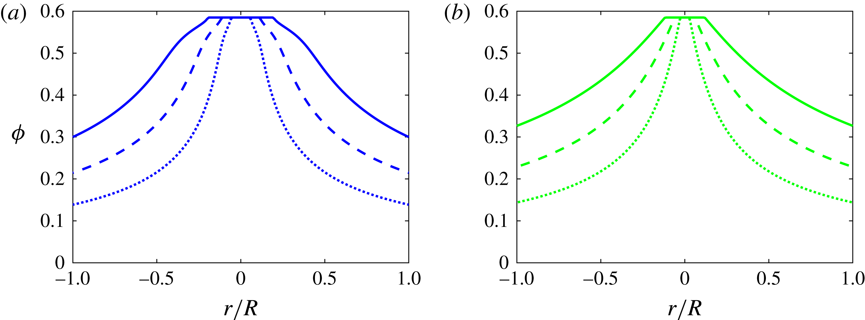
Fully developed concentration profiles with
 ${\it\phi}_{B}=20\,\%$
(dotted line), 30 % (dashed line) and 40 % (solid line) using the rheologies of Boyer et al. (Reference Boyer, Guazzelli and Pouliquen2011a
) (a) and of Morris & Boulay (Reference Morris and Boulay1999) (b).

A.2.1. Steady-state solution
When the flow is fully developed, (A 12) becomes (no flux, thus
 $\boldsymbol{{\rm\nabla}}\boldsymbol{\cdot }{\it\bf\Sigma}^{\boldsymbol{p}}=0$
)
 $$\begin{eqnarray}{\it\lambda}_{2}\frac{\partial \hat{{\it\eta}}_{n}\hat{\dot{{\it\gamma}}}}{\partial \hat{r}}+({\it\lambda}_{2}-{\it\lambda}_{3})\frac{\hat{{\it\eta}}_{n}\hat{\dot{{\it\gamma}}}}{\hat{r}}=0,\end{eqnarray}$$
which, together with the linear variation in
 $r$
of the shear stress
 ${\it\eta}_{s}\dot{{\it\gamma}}$
given by (A 14), provides the friction coefficient (Boyer et al.
Reference Boyer, Guazzelli and Pouliquen2011a
),
 $$\begin{eqnarray}{\it\mu}({\it\phi})=\frac{{\it\eta}_{s}({\it\phi})}{{\it\eta}_{n}({\it\phi})}={\it\mu}_{w}\hat{r}^{(2-{\it\lambda}_{3}/{\it\lambda}_{2})}.\end{eqnarray}$$
Here,
 ${\it\mu}_{w}$
is the friction coefficient at the pipe wall (
 $\hat{r}=1$
).
The suspension flow achieves a jammed state when the volume fraction
 ${\it\phi}$
reaches maximum packing fraction,
 ${\it\phi}_{m}$
. This occurs in a central jammed region of the pipe delimited by
 $\hat{r}_{jam}=[{\it\mu}({\it\phi}_{m})/{\it\mu}_{w}]^{1/(2-{\it\lambda}_{3}/{\it\lambda}_{2})}$
. Outside of this jammed region, the concentration profile is given by inverting the friction function (A 16). Ensuring that the total volume fraction in the pipe corresponds to the initial (uniform) volume fraction
 ${\it\phi}_{B}$
sets the value of
 ${\it\mu}_{w}$
. Both rheological models of Morris & Boulay (Reference Morris and Boulay1999) and Boyer et al. (Reference Boyer, Guazzelli and Pouliquen2011a
) which were described above can be tested. Note that
 ${\it\mu}({\it\phi}_{m})={\it\mu}_{1}$
in the Boyer et al. (Reference Boyer, Guazzelli and Pouliquen2011a
) rheology while
 ${\it\mu}({\it\phi}_{m})=K_{s}/K_{n}$
in the Morris & Boulay (Reference Morris and Boulay1999) rheology. Fully-developed concentration profiles at increasing
 ${\it\phi}_{B}$
are plotted for these two rheologies in figure 19. Both solutions clearly indicate the central plug, or region near the centre where the volume fraction is equal to
 ${\it\phi}_{m}$
.
This frictional approach circumvents the calculation of the singularity at the centre of the pipe which arises when directly integrating (A 15). This method is similar to that used by Lecampion & Garagash (Reference Lecampion and Garagash2014). However, we only consider an incompressible plug at the centre of the pipe, whereas Lecampion & Garagash (Reference Lecampion and Garagash2014) also addressed a central plug with a volume fraction that could exceed
 ${\it\phi}_{m}$
(see their figure 6). The Matlab codes used to calculate the steady profile are given as supplementary material for the two different rheologies of Boyer et al. (Reference Boyer, Guazzelli and Pouliquen2011a
) and Morris & Boulay (Reference Morris and Boulay1999).
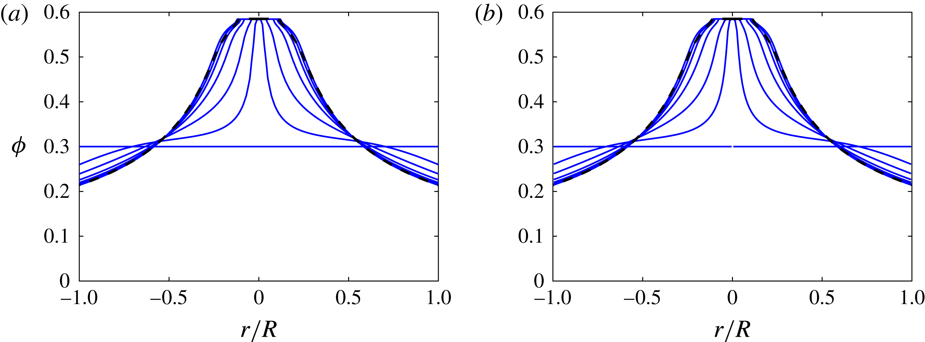
Evolution of the concentration profiles at 30 % and
 $a/R=0.0640$
using the rheology of Boyer et al. (Reference Boyer, Guazzelli and Pouliquen2011a
) for
 $\hat{t}=0,10,30,60,90,120,1000$
using a numerical integration with a
 $O(10^{-6})$
offset (a) and with a constraint on
 ${\it\phi}$
(b). The steady-state solution of § A.2.1 corresponds to the dashed line.

A.2.2. Dynamic solution
To obtain the dynamics, the migration (A 12) must be integrated numerically using the shear rate given by (A 14). In solving these equations, difficulties arise at the centreline of the pipe where the shear rate approaches zero and the volume fraction reaches the maximum packing fraction
 ${\it\phi}_{m}$
. This can be resolved by adding a minuscule,
 $O(10^{-6})$
, constant offset to the shear rate calculated using (A 14). For regions of the flow near the centre, where
 ${\it\phi}$
is close to maximum packing, the constant offset relieves the singularity; for the rest of the domain, the change to the solution is inconsequential. An alternative method places a constraint on the fluxes that prevents the volume fraction from exceeding
 ${\it\phi}_{m}$
. This latter approach utilises the same concept as the frictional approach presented in the preceding section. Both calculations give the same results and reproduce the steady-state solution, as seen in figure 20, with only a small error near the edges of the central plug due to the discretisation and the difficulty in evaluating the rheology near
 ${\it\phi}_{m}$
. The dynamic Matlab codes using the two different rheologies of Boyer et al. (Reference Boyer, Guazzelli and Pouliquen2011a
) and Morris & Boulay (Reference Morris and Boulay1999) are given as supplementary material.
A.2.3. Non-local correction
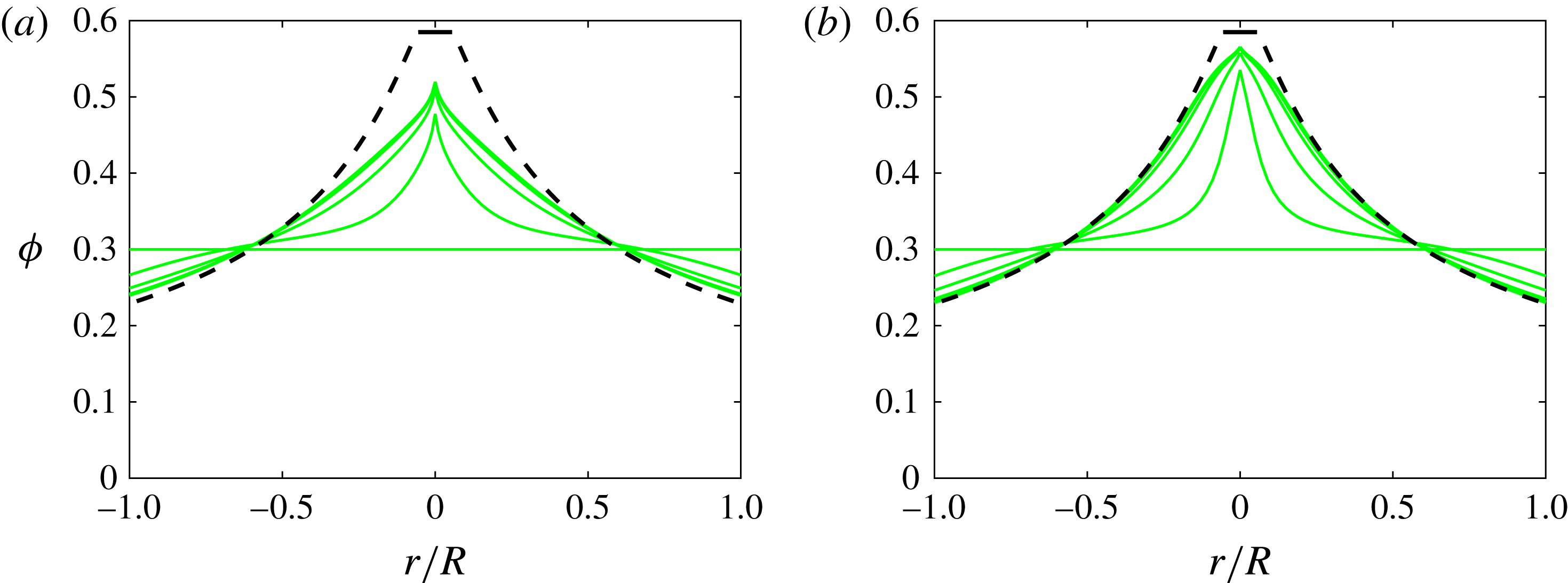
To avoid the singularity and reduce the concentration in the middle of the pipe, multiple researchers have used a ‘non-local’ correction to the stress (see e.g. Nott & Brady Reference Nott and Brady1994; Mills & Snabre Reference Mills and Snabre1995; Morris & Boulay Reference Morris and Boulay1999; Miller & Morris Reference Miller and Morris2006). For regions near the centre of the pipe, where the shear rate approaches zero, the argument is that the finite-sized particles should still experience a finite stress. To correct this shortcoming of the continuum approximation that is inherent within the SBM, a non-local stress correction has been suggested that accounts for the sampling of neighbouring flow regions by the particles over their own size scale. Several variations of the idea have been used and the different non-local stress models have aimed at mimicking this spatial averaging. Following Miller & Morris (Reference Miller and Morris2006), we calculated the volume fraction as a function of radial position while using a non-local correction that depends on the mean shear rate and the particle to the pipe size ratio according to
 $$\begin{eqnarray}\dot{{\it\gamma}}_{NL}=\frac{U}{R}\left(\frac{a}{R}\right)^{m},\end{eqnarray}$$
where the exponent
 $m$
can be adjusted to one or two. As can be seen in figure 21, the concentration in the middle of the pipe diminishes with decreasing
 $m$
. However, the plug region exhibits an a-physical cusp shape. The Matlab codes that employ the non-local correction are given as supplementary material for both the rheology of Boyer et al. (Reference Boyer, Guazzelli and Pouliquen2011a
) and the rheology of Morris & Boulay (Reference Morris and Boulay1999).
Evolution of the concentration profiles at 30 % and
 $a/R=0.0640$
using the rheology of Morris & Boulay (Reference Morris and Boulay1999) for
 $\hat{t}=0,10,30,60,90,120,1000$
using a non-local correction with
 $m=1$
(a) and
 $m=2$
(b). The steady-state solution of § A.2.1 corresponds to the dashed line.