
1. Introduction
Low-Reynolds-number incompressible flow of a single Newtonian fluid in a rigid porous medium is governed, at the microscopic (pore) scale, by Stokes equations. In the absence of rarefaction effects and of any source or sink, they are supplemented with a zero-velocity condition at the solid–fluid interface. Provided the medium can be regarded as statistically homogeneous at a scale much larger than the typical scale of its microstructure, the flow can be described, from a macroscopic point of view, by Darcy's law. This equation relates the local average of the fluid velocity to the gradient of the average pressure via the intrinsic permeability tensor, which depends only on the geometry of the microstructure and accounts for the macroscopic drag on the solid phase. Darcy's law can be formally obtained as the macroscopic momentum equation using various theoretical upscaling methodologies, such as homogenization based on multiple scale expansions or the volume averaging theory (see e.g. Sanchez-Palencia Reference Sanchez-Palencia1980; Whitaker Reference Whitaker1986; Mei, Auriault & Ng Reference Mei, Auriault and Ng1996; Davit et al. Reference Davit2013). As a result of the zero-mass-flux condition at the solid–fluid interface at the underlying pore scale, upscaling also yields a divergence-free average velocity as the macroscopic mass conservation equation. Subject to prescribed conditions at the external boundaries of the macroscopic domain, both equations can be used to solve the macroscopic problem.
In a variety of situations, however, the zero-mass-flux condition at the solid–fluid interface does not apply. This occurs, for example, when the fluid is released from the solid into the pore space or absorbed from the pore space into the solid, due to many possible mechanisms illustrated in the following. It is then a common practice to account for the volume source in the macroscopic mass conservation equation, while using Darcy's law taking the value of the intrinsic permeability, valid in the absence of a source (Lachaud et al. Reference Lachaud, Scoggins, Magin, Meyer and Mansour2017; Vu & Tsotsas Reference Vu and Tsotsas2018). However, the zero velocity at the solid–fluid interface is a key feature in the derivation of the classical form of Darcy's law. There is, a priori, no argument supporting that this equation remains unchanged if non-zero fluxes take place at the interface and, even if a Darcy term remains, the modification or not of the permeability must be carefully addressed. Therefore, it is of interest to determine if such a heuristic formulation is reliable or not. For example, in the presence of interfacial slip, it has been reported that Darcy's law is applicable at the cost that the permeability tensor is no longer intrinsic, as it depends on the Knudsen number, in agreement with the fact that the shear is modified by the existence of slip (Lasseux, Valdés-Parada & Porter Reference Lasseux, Valdés-Parada and Porter2016). When a normal flux is present, one may expect that, if a Darcy term is preserved, the permeability remains intrinsic as in the classical Darcy's law, since the drag is unaltered. However, how the macroscopic momentum equation is affected by the normal inward or outward flow at the pore walls remains to be elucidated.
Fundamentally, the problem under consideration raises the following questions: (i) Is the solenoidal nature of the macroscopic (average) velocity preserved? (ii) Is the Darcy model (macroscopic momentum balance equation) heuristically used for exuding media in some reported works in the literature a physically sound one? (iii) If a Darcy term persists in the macroscopic momentum equation, is the permeability still the intrinsic permeability? These questions are addressed in detail in the following sections. This is a very important problem, from both fundamental and potential applications points of view, which, to the best of our knowledge, has not yet been addressed in the literature. Derivation of a valid macroscopic model in such situations is therefore the purpose of the present work.
In the above description, and in some of the following examples, the solid phase is actually often a nanoporous material. Nevertheless, this nanoporous structure is generally too tight to actively participate in the flow within its volume at the scale of description of interest. Consequently, it can be considered as an apparent continuous solid material allowing fluid transfer between its surface and the neighbouring macropores. An example is provided by the exploitation of tight gas reservoirs, for which natural or induced fracturing is required to access the resource. The gas contained under high pressure in the nanoporous matrix is exuded at the fracture walls. Its flow towards the producing well through the fractures is described, in field-scale simulation models, by Darcy's law (Olorode et al. Reference Olorode, Freeman, Moridis and Blasingame2012; Jiang & Younis Reference Jiang and Younis2015), with a permeability that is deduced from the fracture geometrical characteristics in the absence of surface sources (Mourzenko, Thovert & Adler Reference Mourzenko, Thovert and Adler2018).
Drying or pyrolytic processes also induce interfacial sources, with water vapour or pyrolytic gases produced in the solid and exuded into the pore space. Water can be initially chemically bonded or confined in the liquid state in nanopores. Pyrolytic gases can result from thermal decomposition of biomass or organic compounds, such as kerogen trapped in the nanopores of oil shales. In the latter case, a largely predominant inert mineral matrix prevents the solid from deforming (Elayeb et al. Reference Elayeb, Debenest, Mourzenko and Thovert2017). Darcy's law and the usual intrinsic permeability are universally used in the macroscopic modelling of such situations (see e.g. Erriguible et al. (Reference Erriguible, Bernada, Couture and Roques2006) and Warning, Arquiza & Datta (Reference Warning, Arquiza and Datta2015) for drying, Shepel, Wakili & Hugi (Reference Shepel, Wakili and Hugi2010) for plaster dehydration, and Di Blasi (Reference Di Blasi1994), Larfeldt, Leckner & Melaaen (Reference Larfeldt, Leckner and Melaaen2000), Bryden, Ragland & Rutland (Reference Bryden, Ragland and Rutland2002) and Mahmoudi, Hoffmann & Peters (Reference Mahmoudi, Hoffmann and Peters2014) for pyrolysis).
Chemical reactions can also give rise to non-zero velocities at the solid–fluid interface. Consider, for instance, a carbonaceous solid and the heterogeneous reactions  $\mathrm {O}_2+2\mathrm {C}\rightarrow 2\mathrm {CO}$ (oxidation) or
 $\mathrm {CO}_2+\mathrm {C}\rightarrow 2\mathrm {CO}$ (gasification). In both cases, a single mole of O
 $_2$ or CO
 $_2$ is consumed and two moles of CO are produced. This volume increase, resulting from the net production of gas localized at the solid surface, can be accounted for by a normal velocity directed into the pores. Reactions between gaseous species can result in the same behaviour, if they require a catalyst contained in the solid, such as, for example, the methanation reaction
 $\mathrm {CO}_2+4\mathrm {H}_2\rightarrow \mathrm {CH}_4+2\mathrm {H}_2\mathrm {O}$, or the inverse process of steam reforming (Rönsch et al. Reference Rönsch, Schneider, Matthischke, Schlüter, Götz, Lefebvre, Prabhakaran and Bajohr2016). By converting five moles of gas into three, or conversely, it induces a velocity at the surface directed towards, or away from, the solid, respectively.
Fluxes at the pore–solid interface can also result from phase changes. Interesting examples are provided by the water ice–vapour system, with sublimation and/or condensation at the solid surface. The equilibrium vapour pressure depends on the surface curvature as described by Kelvin's law, giving rise to the isothermal snow ageing metamorphism, with vapour migration from surface sources to surface sinks (Flin et al. Reference Flin, Brzoska, Lesaffre, Coléou and Pieritz2003; Vetter et al. Reference Vetter, Sigg, Singer, Kadau, Herrmann and Schneebeli2010). It also depends on temperature. Thus, in a bubble enclosed in an ice mass subject to a temperature gradient, a water vapour transfer takes place from a surface source by sublimation on the warm side to a surface sink by condensation on the cold side. This phenomenon, in turn, induces the slow migration of the bubble (Shreve Reference Shreve1967; Dadic, Light & Warren Reference Dadic, Light and Warren2010).
In many of the above examples, the solid geometry is subject to evolution, by either mass loss or gain inducing shrinkage or growth. However, the characteristic time associated with the deformation is usually very large compared to that associated with the fluid displacement, so that the flow problem can be treated with a quasi-steady approximation within a fixed geometry. In the water ice–vapour system, for instance, this can be explained by the very large density contrast between solid and gas.
As a generic problem accounting for the above-mentioned situations, in this work interest is focused on the macroscopic description of flow in a porous material resulting from exuding at the solid–fluid interface at the pore scale, i.e. from a non-zero velocity normal component at this interface. The word ‘exuding’ is meant here in a general sense to include fluid release from the surface into the pores or, conversely, absorption from the pores into the solid through the interface. The key question then arises whether Darcy's law is still a valid model at the macroscopic scale, retaining the hypotheses of a Newtonian fluid and creeping incompressible flow conditions.
To address this issue, the article is organized as follows. In § 2, the pore-scale model is presented, the solution of which is illustrated in a simple case, showing that the classical Darcy's law fails and hence highlighting the necessity to derive a macroscopic model. Then § 3 is dedicated to the upscaling of the pore-scale problem, which yields macroscopic mass and momentum transport equations. The former involves a term accounting for the net mass that is released (or absorbed) through the solid–fluid interface, and the latter contains a correction term to Darcy's law. This term involves a local contribution of the exuding effect and a compensation for the periodicity assumption. The model is validated in § 4 by comparisons with pore-scale numerical simulations in a variety of physical situations. Discussion and concluding remarks are provided in § 5.
2. Pore-scale model
In this section, the boundary-value problem under consideration and an illustrative analytical solution in a simple case, justifying the analysis proposed in the following sections, are provided.
2.1. Pore-scale boundary-value problem
Consider a rigid and homogeneous porous medium,  $\mathscr {V}_M$, of typical size
 $L$ and of external macroscopic boundary
 $\partial \mathscr {V}_M$, made of a solid rigid skeleton (
 $\sigma$-phase) and saturated by a single fluid (
 $\beta$-phase) as sketched in figure 1(a). The situation of interest is when the
 $\beta$-phase is either released or absorbed at the solid–fluid interface
 $\mathscr {A}_{\beta \sigma }$. For this process, the
 $\beta$-phase is considered as Newtonian and the flow is assumed to remain in the incompressible creeping regime.
(a) Schematic representation of a porous medium saturated with a single fluid phase along with the averaging domain and characteristic lengths. (b) Position vectors associated with the averaging domain.

Let  $\mathscr {V}$, of measure
 $V$ and size
 $r_0$, in which the region occupied by the
 $\beta$-phase is denoted by
 $\mathscr {V}_\beta$ (of measure
 $V_\beta$), be a subdomain of
 $\mathscr {V}_M$ (
 $\mathscr {V}\subseteq \mathscr {V}_M$) referred to as the averaging domain in the following (see figure 1a). At any point located at
 $\boldsymbol {r}=\boldsymbol {x}+\boldsymbol {y}$ within
 $\mathscr {V}_\beta$, with
 $\boldsymbol {x}$ denoting the position of the centroid of
 $\mathscr {V}$ (see figure 1b), the fluid pressure may be decomposed into the form
 $p|_{\boldsymbol {r}} = \langle p \rangle ^\beta |_{\boldsymbol {r}}+ \tilde {p} |_{\boldsymbol {r}}$ (Gray Reference Gray1975). Application of the gradient operator leads to
 \begin{equation} \left.\boldsymbol{\nabla} p\right|_{\boldsymbol{r}} = \left.\boldsymbol{\nabla} \langle p \rangle^\beta \right|_{\boldsymbol{r}}+ \left. \boldsymbol{\nabla} \tilde{p} \right|_{\boldsymbol{r}}. \end{equation}
In these relationships,  $\langle \psi \rangle ^\beta |_{\boldsymbol {r}}$ denotes the intrinsic average of
 $\psi$ evaluated at
 $\boldsymbol {r}$. The averaging operator at any point
 $\boldsymbol {x}$ is defined as
 \begin{equation} \left. \langle \psi \rangle^\beta \right|_{\boldsymbol{x}} = \frac{1}{V_\beta}\int_{\mathscr{V}_\beta (\boldsymbol{x})} \psi\,\textrm{d}V, \end{equation}
while  $\tilde {\psi }$ represents the deviations of
 $\psi$ with respect to its intrinsic average. In the course of the development, the superficial average defined as
 \begin{equation} \left. \langle \psi \rangle\right|_{\boldsymbol{x}} = \frac{1}{V}\int_{\mathscr{V}_\beta (\boldsymbol{x})} \psi\, \textrm{d}V= \varepsilon \langle \psi \rangle ^\beta \end{equation}
will also be used, with  $\varepsilon$ being the porosity of the medium (
 $\varepsilon =V_\beta /V$), which is assumed to be constant. This is a reasonable assumption that is supported by the consideration of the geometrical homogeneity of the porous medium.
As in the double scale homogenization technique,  $\boldsymbol {x}$ may be understood as the macroscopic (or ‘slow’) variable, having a typical length scale of variation
 $L$, while
 $\boldsymbol {y}$ corresponds to the microscopic (or ‘rapid’) variable, having a characteristic length of variation
 $\ell _\beta$, typical of the pore dimensions (see figure 1b). As for any upscaling procedure, a separation of length scales is assumed, expressed as
 $\ell _\beta \ll r_0 \ll L$.
The gradient of the average pressure evaluated at  $\boldsymbol {r}$ in (2.1) may be further considered using the following Taylor series expansion written in a generic form as
 \begin{equation} \left. {\varPsi} \right|_{\boldsymbol{r}} = \left. {\varPsi} \right|_{\boldsymbol{x}} + \boldsymbol{y}\boldsymbol{\cdot} \boldsymbol{\nabla}\!\left. {\varPsi} \right|_{\boldsymbol{x}} + \tfrac{1}{2} \boldsymbol{y}\boldsymbol{y} \boldsymbol{:} \boldsymbol{\nabla}\boldsymbol{\nabla} \!\left. {\varPsi} \right|_{\boldsymbol{x}}+\cdots. \end{equation}
Performing an order-of-magnitude estimate on the first-order term in this expansion allows one to write
 \begin{equation} \left. {\varPsi} \right|_{\boldsymbol{r}} = \left. {\varPsi} \right|_{\boldsymbol{x}} + {O}\left( \frac{r_0}{L} \Delta {\varPsi} \right), \end{equation}
where  $\Delta {\varPsi }$ represents the characteristic variation of
 ${\varPsi }$ over the length scale
 $L$. Since the order of magnitude of
 $\Delta \varPsi$ can be at most as large as
 $\varPsi$, and as a result of the separation of length scales, it seems reasonable to use the approximation
 ${\varPsi } |_{\boldsymbol {r}} \simeq {\varPsi } |_{\boldsymbol {x}}$. When
 $\varPsi$ represents an average quantity
 $\langle \psi \rangle ^\beta$, and, from now on denoting
 $\langle \psi \rangle ^\beta |_{\boldsymbol {x}}\equiv \langle \psi \rangle ^\beta$, this readily implies
 \begin{equation} \langle \tilde{{\psi}} \rangle ^\beta \simeq 0. \end{equation}
When  $\varPsi$ is taken to be
 $\boldsymbol {\nabla } \langle p \rangle ^\beta$ and when the resulting approximation is introduced in (2.1), the flow problem under consideration can be written in
 $\mathscr {V}$ as
 \begin{gather} \boldsymbol{\nabla} \boldsymbol{\cdot} \boldsymbol{v}=0, \quad \text{in }\mathscr{V}_\beta, \end{gather}
 \begin{gather} \boldsymbol{0} = -\frac{1}{\mu} \boldsymbol{\nabla} \tilde{p} + {\nabla}^2 \boldsymbol{v} -\frac{1}{\mu} \boldsymbol{\nabla} \langle p\rangle^\beta, \quad \text{in }\mathscr{V}_\beta, \end{gather}
 \begin{gather} \boldsymbol{v} =-v_0 \boldsymbol{n}, \quad \text{at} \ \mathscr{A}_{\beta \sigma}. \end{gather}
In these equations,  $\boldsymbol {v}$ is the velocity in the
 $\beta$-phase, whose dynamic viscosity,
 $\mu$, is assumed to be constant. For the sake of simplicity, albeit keeping generality, no body force is considered in the analysis. In the exuding boundary condition at
 $\mathscr {A}_{\beta \sigma }$, (2.7c),
 $v_0$ denotes the rate of production (or consumption) of fluid per unit interfacial area. It is assumed to be a position-dependent but known function of space, a priori, and
 $\boldsymbol {n}$ is the unit normal vector at
 $\mathscr {A}_{\beta \sigma }$ directed from the
 $\beta$-phase to the
 $\sigma$-phase.
Additional boundary conditions at the entrances and exits,  $\mathscr {A}_{\beta e}$, of
 $\mathscr {V}$ must be prescribed in order to complete the problem statement. In a classical homogenization approach, one would certainly consider periodicity at
 $\mathscr {A}_{\beta e}$, as this is the classical way of carrying out the upscaling, assuming locality (Mei et al. Reference Mei, Auriault and Ng1996). However, taking the superficial average of the mass balance equation (2.7a), applying the divergence theorem and making use of the boundary condition at
 $\mathscr {A}_{\beta \sigma }$, yields
 \begin{equation} \frac{1}{V}\int_{\mathscr{A}_{\beta e}} \boldsymbol{n}\boldsymbol{\cdot} \boldsymbol{v}\,\textrm{d}A = \varphi_0 \end{equation}
with
 \begin{equation} \varphi_0=\frac{1}{V}\int_{\mathscr{A}_{\beta\sigma}} v_0\,\textrm{d}A . \end{equation}
Clearly, periodicity on  $\boldsymbol {v}$ at
 $\mathscr {A}_{\beta e}$ is not physically admissible unless
 $\varphi _0=0$. Even though it will be further considered later in the development, the boundary condition at
 $\mathscr {A}_{\beta e}$ is left unspecified at this point. The macroscopic boundary condition over
 $\mathscr {V}_M$ will nevertheless be denoted as
 \begin{equation} \mathscr{G}(\boldsymbol{v},p)=0, \quad \text{at} \ \mathscr{A}_{M\beta e}, \end{equation}
with  $\mathscr {A}_{M\beta e}$ denoting the portion of
 $\partial \mathscr {V}_M$ intersecting the fluid phase. Here, again,
 $\mathscr {G}(\boldsymbol {v},p)$ must be compliant with the equivalent of (2.8) when the entire macroscopic domain is considered.
2.2. Preliminary comments about the interpretation of Darcy's law
At this point of the analysis, it is pertinent to make a clear distinction between the superficial average of the pore-scale velocity (i.e.  $\langle \boldsymbol {v}\rangle$) and another definition of the seepage velocity (denoted
 $\boldsymbol {q}_s$ in the following) that is typically found in the porous media literature. To this end, let
 $\langle \boldsymbol {v}\rangle$ be expressed as follows:
 \begin{equation} \langle \boldsymbol{v}\rangle = \frac{1}{V}\int_{\mathscr{V}_\beta} \boldsymbol{\nabla} \boldsymbol{\cdot} (\boldsymbol{v}\boldsymbol{r})\,\textrm{d}V -\frac{1}{V}\int_{\mathscr{V}_\beta} (\boldsymbol{\nabla} \boldsymbol{\cdot} \boldsymbol{v})\boldsymbol{r}\,\textrm{d}V. \end{equation}
The last term in the above equation is zero due to the solenoidal nature of the pore-scale velocity. Using the divergence theorem in the remaining term, it follows that
 \begin{equation} \langle \boldsymbol{v}\rangle = \boldsymbol{q}_s + \frac{1}{V}\int_{\mathscr{A}_{\beta\sigma}} \boldsymbol{n} \boldsymbol{\cdot} (\boldsymbol{v}\boldsymbol{r})\,\textrm{d}A \end{equation}
with
 \begin{equation} \boldsymbol{q}_s = \frac{1}{V} \int_{\mathscr{A}_{\beta e}} \boldsymbol{n}\boldsymbol{\cdot} \boldsymbol{v} \boldsymbol{r}\,\textrm{d}A. \end{equation}
In the above equations,  $\boldsymbol {q}_s$ is recognized in the porous media literature (see, for instance, Adler Reference Adler1992) as the flux or seepage velocity. This definition of the seepage velocity is intuitively appealing and corresponds to a quantity that is easily measurable in the laboratory, with an empirical origin dating back to H. Darcy's pioneering experiments. In the classical Darcy's law, for which the velocity is zero at the solid–fluid interface, the last term in (2.12) is zero and the result is that
 $\langle \boldsymbol {v}\rangle =\boldsymbol {q}_s=-({1}/{\mu }) {\boldsymbol{\mathsf{K}}}\boldsymbol {\cdot } \boldsymbol {\nabla } \langle p\rangle ^\beta$ so that
 $\langle \boldsymbol {v} \rangle$ or
 $\boldsymbol {q}_s$ may be indifferently employed. However, in the case under study,
 $\boldsymbol {v}=-v_0\boldsymbol {n}$ at
 $\mathscr {A}_{\beta \sigma }$ and (2.12) takes the form
 \begin{equation} \langle \boldsymbol{v}\rangle = \boldsymbol{q}_s - \frac{1}{V}\int_{\mathscr{A}_{\beta\sigma}} v_0\boldsymbol{r}\,\textrm{d}A. \end{equation}
Two important remarks must be made on the expressions for  $\langle \boldsymbol {v} \rangle$ and
 $\boldsymbol {q}_s$. First, it should be noted that
 $\boldsymbol {q}_s$, as given in (2.13), is ill-defined because it explicitly depends on the origin of the system of coordinates when there are net sources in the domain. Conversely, the average velocity,
 $\langle \boldsymbol {v}\rangle$, does not and, consequently, this is the appropriate definition of the macroscopic velocity that must be used in an upscaled equation. Second, the definition of
 $\langle \boldsymbol {v}\rangle$ captures both the mean flow entering or leaving the porous medium (
 $\boldsymbol {q}_s$) and the local fluid displacements resulting from the interfacial sources and/or sinks. These local phenomena must be taken into account for a complete macroscopic description of the flow. The derivations presented in what follows are hence given in terms of
 $\langle \boldsymbol {v}\rangle$ and not of
 $\boldsymbol {q}_s$, which are different in the case under consideration.
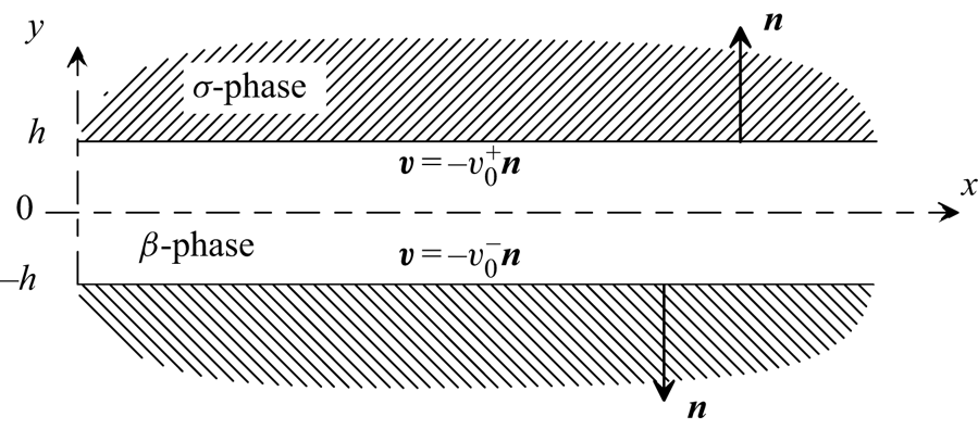
2.3. Solution for a two-dimensional flat channel
Before developing the macroscopic model and in order to illustrate the specific features of the problem, it is instructive to investigate a simple case for which an analytical solution can be achieved. To this end, a two-dimensional periodic layered medium is considered. Its unit cell contains a channel with aperture  $2h$ as illustrated in figure 2. The surface sources are denoted
 $v_0^+$ and
 $v_0^-$ at
 $y=h$ and
 $y=-h$, respectively, and are assumed to be independent of
 $x$, so that
 $\varphi _0=({\varepsilon }/{2h})(v_0^++v_0^-)$.
Two-dimensional flat channel made by a pair of plane parallel plates.

The analytical solution is derived by imposing  $v_x=0$ at
 $x=0$ with the idea that this is a plane of horizontal symmetry resulting from the fact that the channel is open to the atmosphere at both ends along
 $x$. The dimensionless solution for the horizontal and vertical velocities,
 $v_x^*$ and
 $v_y^*$, and pressure,
 $p^*$, in the unit cell is obtained using
 $2h$,
 $v_{ref}=\max (|v_0^+|,|v_0^-|)$ and
 $\mu ({v_{ref}}/{2h})$ as the reference length, velocity and pressure, respectively. This solution is given by
 \begin{gather} v_x^*=\frac{3}{2}\frac{\varphi_0^*}{\varepsilon}(1-4y^{*2} )x^*, \end{gather}
 \begin{gather} v_y^*=-\frac{3}{2}\frac{\varphi_0^*}{\varepsilon}\left(1-\frac{4}{3}y^{*2} \right)y^*-\frac{v_0^{+*}-v_0^{-*}}{2}, \end{gather}
 \begin{gather} p^*=p_1^*+6 \frac{\varphi_0^*}{\varepsilon}(y^{*2} -x^{*2}), \end{gather}
with  $p_1^*$ in (2.15c) being an arbitrary constant. If
 $\varphi _0^*$ is positive, the pressure decreases with
 $x^*$ and from the walls to the channel midplane. The opposite applies if
 $\varphi _0^*$ results in a net sink and
 $p^*$ remains constant if there is no net source or sink.
Although  $v_x^*$ can be identified as a Poiseuille-like solution at each position
 $x^*$, the flow remains two-dimensional. This contrast with respect to the classical flow induced by a pressure gradient along the channel may be better highlighted with the average expressions for
 $v_x^*$,
 $v_y^*$ and
 $p^*$ given by
 \begin{gather} \langle v_x^* \rangle^\beta=-\frac{1}{12} \frac{\partial \langle p^* \rangle^\beta}{\partial x^*}, \end{gather}
 \begin{gather} \langle v_y^* \rangle^\beta= -\frac{v_0^{+*}-v_0^{-*}}{2}, \end{gather}
 \begin{gather} \langle p^*\rangle^\beta=p_2^*-6 \frac{\varphi_0^*}{\varepsilon}x^{*2}, \end{gather}
with  $\langle \psi ^* \rangle ^\beta = \int ^{1/2}_{-1/2} \psi ^*\,{\textrm {d}\kern 0.05em y}$ and
 $p_2^*=p_1^*+\varphi _0^*/(2\varepsilon )$. Equation (2.16a), once multiplied by
 $\varepsilon$, corresponds to the classical Darcy's law, involving the dimensionless permeability,
 $\varepsilon /12$, of the channel system in the
 $x$-direction. For the
 $y$-component of the velocity, no analogy is possible with a Darcy-like flow. Note that this term accounts for the local fluid displacements and remains even if
 $\varphi _0=0$.
This simple example is a clear evidence that the upscaled model accounting for the presence of surface sources and/or sinks at the solid–fluid interfaces cannot be reduced, in general, to Darcy's law.
3. Upscaling
In this section, the derivation of a macroscopic model for the flow problem given in (2.7) is proposed. The macroscale mass equation is obtained following the classical volume averaging method (Whitaker Reference Whitaker1999). However, for the derivation of the upscaled momentum equation, an approach inspired by the adjoint homogenization method recently proposed by Bottaro (Reference Bottaro2019) is used.
3.1. Mass balance equation
In order to derive the macroscopic mass equation, it is convenient to recall the result given in (2.8) and use the relationship reported by Slattery (Reference Slattery1967),
 \begin{equation} \frac{1}{V}\int_{\mathscr{A}_{\beta e}} \boldsymbol{n}\boldsymbol{\cdot} \boldsymbol{v}\,\textrm{d}A = \boldsymbol{\nabla} \boldsymbol{\cdot} \langle \boldsymbol{v}\rangle , \end{equation}
in order to obtain
 \begin{equation} \boldsymbol{\nabla} \boldsymbol{\cdot} \langle \boldsymbol{v}\rangle = \varphi_0, \end{equation}
with  $\varphi _0$ given in (2.9). It should be noted that, except when
 $\varphi _0=0$, this result contrasts with the macroscopic mass balance equation obtained while deriving the classical Darcy's law with a zero velocity at
 $\mathscr {A}_{\beta \sigma }$ (Whitaker Reference Whitaker1986, Reference Whitaker1999) or when a slip flow boundary condition is considered (Lasseux et al. Reference Lasseux, Valdés-Parada and Porter2016). In other words, a consequence of the conservation of mass within the averaging domain is that
 $\langle \boldsymbol {v}\rangle$ has a non-solenoidal character, despite the fact that the flow is incompressible at the underlying pore scale. This non-solenoidal nature of the average velocity is an important modification to the classical Darcy model, as it accounts for the mass entering/exiting the system through the solid–fluid interface. At this point, the macroscopic model must be complemented with the momentum balance equation as proposed in the following subsection.
3.2. Momentum equation
An efficient and simple way to derive a macroscopic form of the momentum equation is to make use of the adjoint method proposed by Bottaro (Reference Bottaro2019). To this purpose, an adjoint problem can be conveniently defined with the minimum requirements as follows:
 \begin{gather} \boldsymbol{\nabla} \boldsymbol{\cdot} {\boldsymbol{\mathsf{D}}}=\boldsymbol{0}, \quad \text{in }\mathscr{V}_\beta, \end{gather}
 \begin{gather} \boldsymbol{0}=- \boldsymbol{\nabla} \boldsymbol{d} + \nabla^2 {\boldsymbol{\mathsf{D}}} +{\boldsymbol{\mathsf{I}}}, \quad \text{in }\mathscr{V}_\beta, \end{gather}
 \begin{gather} {\boldsymbol{\mathsf{D}}}=\boldsymbol{0}, \quad \text{at} \ \mathscr{A}_{\beta \sigma}. \end{gather}
Again, boundary conditions for  ${\boldsymbol{\mathsf{D}}}$ and
 $\boldsymbol {d}$ at
 $\mathscr {A}_{\beta e}$ are necessary for this problem to be well-posed. However, they are not specified here, as they are not required at this point of the development.
The derivation is carried out by adding the product of (2.7a) by  $\boldsymbol {d}$ to (2.7b) pre-multiplied by
 ${\boldsymbol{\mathsf{D}}}^{\textrm {T}}$. Forming the superficial average of the result leads to
 \begin{equation} \left\langle \boldsymbol{d} \boldsymbol{\nabla} \boldsymbol{\cdot} \boldsymbol{v} \right\rangle+ \left\langle {\boldsymbol{\mathsf{D}}}^{\textrm{T}}\boldsymbol{\cdot} \left( -\frac{1}{\mu} \boldsymbol{\nabla} \tilde{p}+\nabla^2 \boldsymbol{v} \right) \right\rangle =\frac{1}{\mu} \langle {\boldsymbol{\mathsf{D}}}^{\textrm{T}}\rangle \boldsymbol{\cdot} \boldsymbol{\nabla} \langle p\rangle^\beta. \end{equation}
The three terms on the left-hand side of the above equation can be respectively rewritten as
 \begin{gather} \langle \boldsymbol{d} \boldsymbol{\nabla} \boldsymbol{\cdot} \boldsymbol{v} \rangle= \langle \boldsymbol{\nabla} \boldsymbol{\cdot}(\boldsymbol{vd}) \rangle -\langle \boldsymbol{v}\boldsymbol{\cdot} \boldsymbol{\nabla} \boldsymbol{d} \rangle, \end{gather}
 \begin{gather} -\frac{1}{\mu} \langle {\boldsymbol{\mathsf{D}}}^{\textrm{T}}\boldsymbol{\cdot} \boldsymbol{\nabla} \tilde{p} \rangle= -\frac{1}{\mu} \langle \boldsymbol{\nabla} \boldsymbol{\cdot} ( \tilde{p}{\boldsymbol{\mathsf{D}}}) \rangle, \end{gather}
 \begin{gather} \langle {\boldsymbol{\mathsf{D}}}^{\textrm{T}}\boldsymbol{\cdot} \nabla^2 \boldsymbol{v} \rangle= \langle \boldsymbol{v} \boldsymbol{\cdot} \nabla^2 {\boldsymbol{\mathsf{D}}}\rangle+ \langle \boldsymbol{\nabla} \boldsymbol{\cdot} ( \boldsymbol{\nabla} \boldsymbol{v}\boldsymbol{\cdot} {\boldsymbol{\mathsf{D}}}-\boldsymbol{v} \boldsymbol{\cdot} (\boldsymbol{\nabla} {\boldsymbol{\mathsf{D}}})^{\textrm{T}1}) \rangle. \end{gather}
Equation (3.5b) is obtained while taking into account the divergence-free property of  ${\boldsymbol{\mathsf{D}}}$. Note that, in (3.5c), the superscript
 $\textrm {T}1$ denotes the transpose operator on the third-order tensor
 $\boldsymbol {\nabla } {\boldsymbol{\mathsf{D}}}$, which permutes the first and second indices, i.e.
 $(\boldsymbol {\nabla } {\boldsymbol{\mathsf{D}}} )^{\textrm {T}1}_{ijk}=(\boldsymbol {\nabla } {\boldsymbol{\mathsf{D}}} )_{jik}$. Introducing these expressions into (3.4) and making use of (3.3b) allows
 $\langle \boldsymbol {v} \rangle$ to be expressed as
 \begin{equation} \langle \boldsymbol{v} \rangle= -\frac{1}{\mu} \langle {\boldsymbol{\mathsf{D}}}^{\textrm{T}} \rangle \boldsymbol{\cdot} \boldsymbol{\nabla} \langle p \rangle^\beta + \left \langle \boldsymbol{\nabla} \boldsymbol{\cdot} \left[\boldsymbol{v} \boldsymbol{\cdot} ( {\boldsymbol{\mathsf{I}}} \boldsymbol{d}-\left( \boldsymbol{\nabla} {\boldsymbol{\mathsf{D}}} \right)^{\textrm{T}1} )+\left( -\frac{1}{\mu} \tilde{p}{\boldsymbol{\mathsf{I}}}+\boldsymbol{\nabla} \boldsymbol{v} \right)\boldsymbol{\cdot} {\boldsymbol{\mathsf{D}}} \right] \right \rangle. \end{equation}
This last expression can be reformulated using the divergence theorem together with the boundary conditions for  $\boldsymbol {v}$ and
 ${\boldsymbol{\mathsf{D}}}$ at
 $\mathscr {A}_{\beta \sigma }$ given in (2.7c) and (3.3c) in order to obtain
 \begin{align} \langle \boldsymbol{v}\rangle &= -\frac{1}{\mu} \left\langle {\boldsymbol{\mathsf{D}}}\right\rangle^{\textrm{T}} \boldsymbol{\cdot} \boldsymbol{\nabla} \langle p\rangle^\beta -\frac{1}{V} \int_{\mathscr{A}_{\beta\sigma} } v_0 \left( \boldsymbol{d} - \boldsymbol{nn} \boldsymbol{:} \boldsymbol{\nabla} {\boldsymbol{\mathsf{D}}} \right) \,\textrm{d}A \nonumber\\ &\quad +\frac{1}{V} \int_{\mathscr{A}_{\beta e}} \boldsymbol{n}\boldsymbol{\cdot} \left( -\frac{1}{\mu}\tilde{p}{\boldsymbol{\mathsf{I}}} +\boldsymbol{\nabla} \boldsymbol{v}\right)\boldsymbol{\cdot} {\boldsymbol{\mathsf{D}}}\,\textrm{d}A -\frac{1}{V} \int_{\mathscr{A}_{\beta e}} \boldsymbol{n}\boldsymbol{\cdot} [\boldsymbol{v} \boldsymbol{\cdot} ( - {\boldsymbol{\mathsf{I}}} \boldsymbol{d} +(\boldsymbol{\nabla} {\boldsymbol{\mathsf{D}}})^{\textrm{T}1} ) ]\,\textrm{d}A. \end{align}
Here, the fact that  $\boldsymbol {nn} \boldsymbol {:} (\boldsymbol {\nabla } {\boldsymbol{\mathsf{D}}})^{\textrm {T}1}=\boldsymbol {nn} \boldsymbol {:} \boldsymbol {\nabla } {\boldsymbol{\mathsf{D}}}$ was taken into account as a result of the symmetry property of the tensor
 $\boldsymbol {n} \boldsymbol {n}$. It must be noted that (3.7) is valid whatever boundary conditions at
 $\mathscr {A}_{\beta e}$ are imposed for both the physical (2.7) and adjoint (3.3) problems and that the only approximation is that associated with (2.5).
To make further progress towards a closed form of this macroscopic momentum equation, it is now assumed that the porous structure can be assimilated to a periodic one and that  $v_0$ is also periodic. Under theses circumstances,
 $\mathscr {V}$ is selected as the smallest periodic unit cell satisfying these properties. Moreover, periodic boundary conditions on
 ${\boldsymbol{\mathsf{D}}}$ and
 $\boldsymbol {d}$ can be considered for the adjoint problem, as this does not imply any physical or mathematical contradiction. This choice is retained in the remainder of the development. Nevertheless, appropriate boundary conditions at
 $\mathscr {A}_{\beta e}$ for the physical problem are still required, keeping in mind that periodicity on
 $\boldsymbol {v}$ is incompatible with (2.8) when
 $\varphi _0\neq 0$. To handle this situation, it is proposed, as an ansatz, to consider periodic boundary conditions for both
 $\boldsymbol {v}$ and
 $\tilde {p}$ at
 $\mathscr {A}_{\beta e}$ and then compensate for this assumption, as explained below. For the moment, it suffices to note that, on the basis of periodic boundary conditions for both the physical and adjoint problems, (3.7) reduces to
 \begin{equation} \langle \boldsymbol{v}\rangle = -\frac{1}{\mu} \left\langle {\boldsymbol{\mathsf{D}}}^{\textrm{T}}\right\rangle \boldsymbol{\cdot} \boldsymbol{\nabla} \langle p\rangle^\beta -\frac{1}{V} \int_{\mathscr{A}_{\beta\sigma} } v_0 \boldsymbol{d}\,\textrm{d}A + \frac{1}{V} \int_{\mathscr{A}_{\beta\sigma} } v_0 \boldsymbol{nn} \boldsymbol{:} \boldsymbol{\nabla} {\boldsymbol{\mathsf{D}}} \,\textrm{d}A. \end{equation}
An additional simplification can be made regarding the last term in the above expression for  $\langle \boldsymbol {v} \rangle$. Taking into account the fact that
 $\boldsymbol {v}$ is a solenoidal field allows one to write
 \begin{equation} \langle {\boldsymbol{\mathsf{D}}}^{\textrm{T}} \boldsymbol{\cdot} (\boldsymbol{\nabla} \boldsymbol{\cdot}(\boldsymbol{\nabla} \boldsymbol{v})^{\textrm{T}}) \rangle = \langle \boldsymbol{\nabla} \boldsymbol{\cdot} ((\boldsymbol{\nabla} \boldsymbol{v})^{\textrm{T}} \boldsymbol{\cdot} {\boldsymbol{\mathsf{D}}} - \boldsymbol{v \boldsymbol{\cdot} \boldsymbol{\nabla} {\boldsymbol{\mathsf{D}}}} ) \rangle = \boldsymbol{0}. \end{equation}
Applying the divergence theorem to the term in the middle of (3.9) leads to
 \begin{equation} \frac{1}{V} \int_{\mathscr{A}_{\beta\sigma} } v_0 \boldsymbol{nn} \boldsymbol{:} \boldsymbol{\nabla} {\boldsymbol{\mathsf{D}}}\,\textrm{d}A +\frac{1}{V} \int_{\mathscr{A}_{\beta e}} \boldsymbol{n}\boldsymbol{\cdot} \left( \boldsymbol{\nabla} \boldsymbol{v}\right)^{\textrm{T}}\boldsymbol{\cdot} {\boldsymbol{\mathsf{D}}}\,\textrm{d}A -\frac{1}{V} \int_{\mathscr{A}_{\beta e}} \boldsymbol{n}\boldsymbol{\cdot} \left( \boldsymbol{v} \boldsymbol{\cdot} \boldsymbol{\nabla} {\boldsymbol{\mathsf{D}}} \right)\,\textrm{d}A = \boldsymbol{0}. \end{equation}
When periodic boundary conditions for both  $\boldsymbol {v}$ and
 ${\boldsymbol{\mathsf{D}}}$ are considered, the two last terms on the left-hand side of this last relationship are zero, which means that
 \begin{equation} \frac{1}{V} \int_{\mathscr{A}_{\beta\sigma} } v_0 \boldsymbol{nn} \boldsymbol{:} \boldsymbol{\nabla} {\boldsymbol{\mathsf{D}}}\,\textrm{d}A = \boldsymbol{0}. \end{equation}
This allows (3.8) to be simplified to
 \begin{equation} \langle \boldsymbol{v}\rangle = -\frac{1}{\mu} \left\langle {\boldsymbol{\mathsf{D}}}\right\rangle^\textrm{T} \boldsymbol{\cdot} \boldsymbol{\nabla} \langle p\rangle^\beta -\frac{1}{V} \int_{\mathscr{A}_{\beta\sigma} } v_0 \boldsymbol{d}\,\textrm{d}A. \end{equation}
It must be kept in mind that this form is an approximation of  $\langle \boldsymbol {v} \rangle$, as a result of the application of periodic boundary conditions for
 $\boldsymbol {v}$ at
 $\mathscr {A}_{\beta e}$. Moreover, at this stage of the derivations, an important point remains to be carefully addressed. Indeed, the adjoint problem for
 ${\boldsymbol{\mathsf{D}}}$ and
 $\boldsymbol {d}$ given in (3.3), complemented with periodic boundary conditions, remains ill-posed, as
 $\boldsymbol {d}$ can only be determined to within an arbitrary additive constant, and this leaves the expression of
 $\langle \boldsymbol {v} \rangle$ undetermined due to the last integral term on the right-hand side of (3.12). When
 $v_0$ is uniformly zero, i.e. when the problem reduces to the derivation of Darcy's law, it can be shown that an additional constraint can be imposed on
 $\boldsymbol {d}$ by setting
 $\langle \boldsymbol {d} \rangle ^\beta$ equal to an arbitrary constant for the adjoint problem to be well-posed. This is due to the fact that, in this particular case, the closed macroscopic momentum equation only involves
 $\langle {\boldsymbol{\mathsf{D}}} \rangle$ and that the field of
 ${\boldsymbol{\mathsf{D}}}$ is insensitive to any additive constant superimposed onto the field of
 $\boldsymbol {d}$. Indeed, the only source of the physical problem originates from the gradient of the average pressure reflected in the source term
 ${\boldsymbol{\mathsf{I}}}$ in (3.3b). However, when a non-zero exuding flux is present,
 $\boldsymbol {d}$ must be uniquely defined in (3.12) to obtain a closed expression for
 $\langle \boldsymbol {v} \rangle$. This feature results from the fact that periodic boundary conditions have been considered for
 $\boldsymbol {v}$, while the solution for
 $\langle \boldsymbol {v} \rangle$ depends on both the internal surface source or sink,
 $v_0$, and the macroscopic boundary conditions.
To circumvent this difficulty, it is convenient to consider the decomposition of  $\boldsymbol {d}$ under its intrinsic average
 $\boldsymbol {\lambda }= \langle \boldsymbol {d} \rangle ^\beta$ and deviation
 $\boldsymbol {d}_1=\tilde {\boldsymbol {d}}$ as
 \begin{equation} \boldsymbol{d}= \boldsymbol{\lambda}+\boldsymbol{d}_1. \end{equation}
Keeping in mind that, within the periodic unit cell,  $\mathscr {V}$, one has
 $\langle \boldsymbol {d}_1 \rangle ^\beta = \boldsymbol {0}$ (see (2.6) with
 $\tilde {\psi }=\boldsymbol {d}_1$) and that
 $\boldsymbol {\lambda }$ can be considered as a constant (see (2.5) with
 $\varPsi =\boldsymbol {\lambda }$ together with the ensuing approximation), the adjoint problem for
 $\boldsymbol {d}_1$ and
 ${\boldsymbol{\mathsf{D}}}$ can be written as
 \begin{gather} \boldsymbol{\nabla} \boldsymbol{\cdot} {\boldsymbol{\mathsf{D}}}=\boldsymbol{0}, \quad \text{in } \mathscr{V}_\beta, \end{gather}
 \begin{gather} \boldsymbol{0}=- \boldsymbol{\nabla} \boldsymbol{d}_1 + \nabla^2 {\boldsymbol{\mathsf{D}}} +{\boldsymbol{\mathsf{I}}}, \quad \text{in }\mathscr{V}_\beta, \end{gather}
 \begin{gather} {\boldsymbol{\mathsf{D}}}=\boldsymbol{0} \quad \text{at} \ \mathscr{A}_{\beta \sigma}, \end{gather}
 \begin{gather} \psi(\boldsymbol{r}+\boldsymbol{l}_i)=\psi(\boldsymbol{r}), \quad i=1,2,3,\ \psi=\boldsymbol{d}_1, {\boldsymbol{\mathsf{D}}}, \end{gather}
 \begin{gather} \langle \boldsymbol{d}_1\rangle^\beta =\boldsymbol{0}, \end{gather}
where  $\boldsymbol {l}_i$ are the periodic lattice vectors of
 $\mathscr {V}$. This problem exactly corresponds to the closure problem (
 ${\boldsymbol{\mathsf{D}}}$ and
 $\boldsymbol {d}_1$ being the closure variables) involved in the derivation of the classical Darcy's law from which the intrinsic permeability tensor
 ${\boldsymbol{\mathsf{K}}}$ is given by Whitaker (Reference Whitaker1986, Reference Whitaker1999), Mei et al. (Reference Mei, Auriault and Ng1996) and Mei & Vernescu (Reference Mei and Vernescu2010):
 \begin{equation} {\boldsymbol{\mathsf{K}}}=\langle {\boldsymbol{\mathsf{D}}} \rangle. \end{equation}
The introduction of the decomposition for  $\boldsymbol {d}$ into (3.12) while taking into account that K is a symmetric tensor (see e.g. Lasseux & Valdés-Parada Reference Lasseux and Valdés-Parada2017) yields
 \begin{equation} \langle \boldsymbol{v}\rangle = -\frac{1}{\mu} {\boldsymbol{\mathsf{K}}} \boldsymbol{\cdot} \boldsymbol{\nabla} \langle p\rangle^\beta +\boldsymbol{v}_s, \end{equation}
where the vector  $\boldsymbol {v}_s$, denoting the correction velocity to Darcy's law due to the surface source or sink,
 $v_0$, is defined as
 \begin{equation} \boldsymbol{v}_s=\underbrace{-\frac{1}{V} \int_{\mathscr{A}_{\beta\sigma} } v_0 \boldsymbol{d}_1\,\textrm{d}A}_{\boldsymbol{v}_{d}}\underbrace{-\boldsymbol{\lambda} \varphi_0}_{\boldsymbol{v}_\lambda}. \end{equation}
It should be noted that both  ${\boldsymbol{\mathsf{K}}}$ and
 $\boldsymbol {v}_d$ are obtained from the same closure (adjoint) problem that is intrinsic to the structure under consideration and it corresponds to the same closure problem yielding
 ${\boldsymbol{\mathsf{K}}}$ in the classical Darcy's law. This is novel in the volume averaging method, where it is usually required to produce a distinct closure problem for each source in the pore-scale model. In addition, it should be noted that
 $\boldsymbol {v}_d$, like
 ${\boldsymbol{\mathsf{K}}}$, is independent of the fluid viscosity, but, unlike
 ${\boldsymbol{\mathsf{K}}}$, it is unmodified in a homothetic change of scale of the microstructure.
To clarify the physical meaning of the terms involved in the macroscopic momentum equation (3.16), it is instructive to rewrite it in the following alternative form
 \begin{equation} -\frac{{\boldsymbol{\mathsf{K}}}}{\mu}\boldsymbol{\cdot} \boldsymbol{\nabla} \langle p\rangle^\beta = -\frac{{\boldsymbol{\mathsf{K}}}}{\mu}\boldsymbol{\cdot}\frac{1}{V_\beta}\int_{\mathscr{A}_{\beta \sigma}} \boldsymbol{n}\boldsymbol{\cdot} {\boldsymbol{\mathsf{T}}}\,\textrm{d}A = \boldsymbol{v}_1=\langle \boldsymbol{v}\rangle - \boldsymbol{v}_s, \end{equation}
where  ${\boldsymbol{\mathsf{T}}}$ is the total stress tensor (
 ${\boldsymbol{\mathsf{T}}}=-p{\boldsymbol{\mathsf{I}}}+\mu (\boldsymbol {\nabla } \boldsymbol {v}+ (\boldsymbol {\nabla } \boldsymbol {v})^{\textrm {T}})$). In this formulation,
 $\boldsymbol {v}_1$, which identifies as the Darcy term, corresponds to the average contribution of the microscale flow field that induces a force on the solid phase (which translates into the macroscopic pressure gradient). Conversely,
 $\boldsymbol {v}_s$ is the contribution that does not induce such a force but is nevertheless not zero due to the local fluid displacements.
In the expression of  $\boldsymbol {v}_s$, the first term (i.e.
 $\boldsymbol {v}_d$) accounts for the local effect of
 $v_0$ whereas the second term (i.e.
 $\boldsymbol {v}_\lambda$) is a compensation of the effect of the periodic boundary condition applied to
 $\boldsymbol {v}$ at the level of the unit cell. The idea here is that
 $\boldsymbol {\lambda }$ can be computed from (3.16) with
 $\langle \boldsymbol {v}\rangle$ obtained by solving the pore-scale flow problem in a domain potentially significantly smaller than
 $\mathscr {V}_M$ with the same macroscopic boundary condition (see (2.10)). If such reduction is not possible, then it should be evaluated from a flow solution over the entire domain. Nevertheless, as illustrated in § 4 below,
 $\boldsymbol {\lambda }$ has no significant contribution in many circumstances, even if it can be crucial in some very specific cases. The correction term
 $\boldsymbol {v}_\lambda$ in
 $\boldsymbol {v}_s$ does not even exist when
 $\varphi _0=0$ and this is consistent with the fact that, in that case, periodic boundary conditions for
 $\boldsymbol {v}$ at
 $\mathscr {A}_{\beta e}$ are physically admissible.
A particular feature of  $\boldsymbol {v}_d$ must be pointed out when the structure is non-percolating in a direction,
 $\boldsymbol {e}_k$, of space. In such circumstances, the projection of the closure problem on
 $\boldsymbol {e}_k$ admits the unique solution
 \begin{equation} {\boldsymbol{\mathsf{D}}} \boldsymbol{\cdot} \boldsymbol{e}_k=\boldsymbol{0} \end{equation}
and consequently
 \begin{equation} \boldsymbol{d}_1\boldsymbol{\cdot} \boldsymbol{e_k}=\left(\boldsymbol{r}-\boldsymbol{r}_G \right)\boldsymbol{\cdot} \boldsymbol{e}_k, \end{equation}
with  $\boldsymbol {r}_G$ being the barycentre of
 $\mathscr {V}_\beta$. From (3.19b), it appears that
 $\boldsymbol {v}_d\boldsymbol {\cdot } \boldsymbol {e}_k$ is the first moment of
 $v_0$ in the
 $\boldsymbol {e}_k$-direction. Hence, an average velocity may be induced in a non-percolating direction of the medium in the absence of a macroscopic pressure gradient, as already noted in the case of the flat channel (see (2.16b)). This is further illustrated in § 4.
The fact that the correction to Darcy's law given in (3.16) is a vector implies that, for situations in which the microstructure and the distribution of  $v_0$ are both isotropic,
 $\boldsymbol {v}_s$ should be zero due to the absence of a privileged direction. Isotropy can also result from statistical reasons, such as the averaging of the randomness in real media. In addition,
 $\boldsymbol {v}_d$ may also be evanescent because of an uncorrelated combination of
 $\boldsymbol {d}_1$ and
 $v_0$. In other words,
 $\boldsymbol {v}_s$ plays a role only if there is some spatial alignment in the local geometrical and/or fluid exuding distribution properties, in particular, when
 $v_0$ presents some kind of polarization between releasing and absorbing interfaces. Moreover, an order-of-magnitude estimate can be performed on
 $\boldsymbol {v}_d$ and
 $\boldsymbol {v}_\lambda$ as reported in appendix A. It shows that both
 $\boldsymbol {v}_d$ and
 $\boldsymbol {v}_\lambda$ are, at most, of order
 $v_0$.
As a summary, the upscaled (or macroscopic) model describing flow in porous media of a Newtonian fluid in the creeping incompressible regime, induced by a rigid and homogeneous exuding solid matrix, is given by
 \begin{gather} \boldsymbol{\nabla} \boldsymbol{\cdot} \langle \boldsymbol{v}\rangle =\varphi_0, \end{gather}
 \begin{gather}\langle \boldsymbol{v} \rangle = - \frac{{\boldsymbol{\mathsf{K}}}}{\mu}\boldsymbol{\cdot} \boldsymbol{\nabla} \langle p\rangle^\beta +\boldsymbol{v}_s, \end{gather}
in which  $\varphi _0$ and
 $\boldsymbol {v}_s$ are given by (2.9) and (3.17), respectively, and this represents the salient result of this work. Clearly, the macroscopic momentum equation (3.20b) differs from Darcy's law by the correction term
 $\boldsymbol {v}_s$, while
 $\langle \boldsymbol {v} \rangle$ is not a divergence-free field, except when
 $\varphi _0=0$.
4. Results
The purpose of this section is to assess the validity of the macroscale model derived in § 3 for a variety of situations. First, flow in two geometries of corrugated two-dimensional channels is considered for three configurations of  $v_0$ at the solid–fluid interface. Second, flow in both isotropic and anisotropic two-dimensional model porous media is analysed. Finally, the case of exuding within spherical bubbles is investigated, a situation that may be thought of as a simple representation of the migration of water vapour bubbles in ice.
In all the situations studied here, the reference macroscale velocity and pressure results are those obtained from averaging the numerical solution of the governing flow equations at the pore scale carried out in  $\mathscr {V}_M$. The pore-scale numerical simulations (PSNS) of the flow problem, as well as the solutions of the closure problem given in (3.14) and of the upscaled model (UM) are carried out using the finite element solver Comsol Multiphysics 5.5. The smoothed aggregation algebraic multigrid solver was chosen for the fluid flow variables considering preconditioning. In addition, typical tests of convergence in terms of the relative tolerance and number of mesh elements were performed so that the results presented here are independent of these numerical degrees of freedom.
For the developments reported below, it is convenient to introduce the following dimensionless variables and parameters:
 \begin{gather} \boldsymbol{r}^*= \frac{\boldsymbol{r}}{\ell_{cell}}, \quad \boldsymbol{v}^*= \frac{\boldsymbol{v}}{v_{ref}}, \quad v_0^* = \frac{v_0}{v_{ref}}, \quad p^* = \frac{p \ell_{cell}}{\mu v_{ref}}, \quad \varphi_0^* = \frac{\varphi_0 \ell_{cell}}{v_{ref}}, \nonumber\\ {\boldsymbol{\mathsf{K}}}^*= \frac{{\boldsymbol{\mathsf{K}}}}{\ell_{cell}^2}, \quad \boldsymbol{\lambda}^* = \frac{\boldsymbol{\lambda}}{\ell_{cell}}, \quad \boldsymbol{d}_1^* = \frac{\boldsymbol{d}_1}{\ell_{cell}}, \quad {\boldsymbol{\mathsf{D}}}^* = \frac{{\boldsymbol{\mathsf{D}}}}{\ell_{cell}^2}. \end{gather}
Here  $v_{ref}=\max (|v_0|)$ whereas
 $\ell _{cell}$ is the length of the geometrical periodic unit cell used to construct the solution domain.
Before presenting the numerical results, the analytical solution obtained from the macroscopic model in the case of the flat channel is compared to the flow solution reported in § 2.3, keeping the same conditions. In that case,  $\ell _{cell}=2h$ and the analytical solution of (3.14) for
 ${\boldsymbol{\mathsf{D}}}^*$ and
 $\boldsymbol {d}_1^*$ is given by
 \begin{gather} D^*_{xx}=\frac{1}{2}\left( -y^{*2}+\frac{1}{2} \right), \quad D^*_{yx}=0, \quad d_{1x}^*=0, \end{gather}
 \begin{gather} D^*_{xy}=0, \quad D^*_{yy}=0, \quad d_{1y}^*=y^*. \end{gather}
Note that the results in (4.2b) correspond to the solution in (3.19), as expected. Once these results are inserted into (3.16), it yields
 \begin{gather} \langle v_x^* \rangle=-\frac{\varepsilon}{12} \frac{\partial \langle p^* \rangle ^\beta}{\partial x^*}, \end{gather}
 \begin{gather} \langle v_y^* \rangle=-\frac{\varepsilon(v_0^{+*}-v_0^{-*})}{2}. \end{gather}
Combining the macroscopic mass and momentum equations (3.20) leads to the following average dimensionless pressure equation:
 \begin{equation} {-}\frac{\varepsilon}{12}\frac{\partial^2\langle p^* \rangle^\beta}{\partial x^{*2}}=\varphi_0^*=\varepsilon \left(v_0^{+*}+v_0^{-*}\right). \end{equation}
The solution of this equation is obtained by considering that  $\langle v_x^* \rangle =0$ (i.e.
 $\partial \langle p^* \rangle ^\beta /\partial x^*=0$) at
 $x^*=0$ and it can be written as
 \begin{equation} \langle p^*\rangle^\beta=p^*_2-6 \frac{\varphi_0^*}{\varepsilon}x^{*2}, \end{equation}
with  $p_2^*$ being an arbitrary constant. The results given in (4.3) and (4.4b) coincide with those obtained from the flow solution (see (2.16)). In particular,
 $\boldsymbol {v}_\lambda ^*$ is zero and the result from the macroscopic model is exact in that case.
4.1. Flow in corrugated channels
In this section, two types of two-dimensional channels, for which the macroscopic domain,  $\mathscr {V}_M$, is composed of
 $N$ repetitions (
 $N=11$ here) along
 $x$ of a geometrical periodic unit cell, are considered. This geometry may be viewed as a simple model to study flow in exuding fractures (cf. Rasoulzadeh et al. Reference Rasoulzadeh, Yekta, Deng and Ghahfarokhi2020). For the first channel geometry, namely the wavy channel, the lower wall at
 $y^*=0$ is flat, while the upper wall follows the oscillatory function
 $y^* = 0.35+0.25\cos (2{\rm \pi} x^*)$. The developed dimensionless length of the upper wall is denoted by
 $A_{upper}^*$. The second type of geometry, referred to as the shark-fin channel, is such that the lower wall is corrugated and not symmetric. It presents a positive undulation over the baseline
 $y^*=0$ while the upper wall is flat, positioned at
 $y^*=1$. In the following numerical evaluations, the dimensionless height of the unit cell is taken equal to the maximum dimensionless channel aperture, i.e. 0.6 and 1 for the wavy and shark-fin channels, respectively. The interest is to examine the following four configurations.
(i) Case a:
 $v_0^*=1$ at the upper wall and $v_0^* = -A_{upper}^*$ at the lower wall in the wavy channel, so that $\varphi _0^*=0$.
(ii) Case b:
$v_0^*=1$ at $\mathscr {A}_{\beta \sigma }$ in the wavy channel.(iii) Case c:
$v_0^*=1$ at the solid–fluid interfaces located in the right half and $v_0^*=0$ in the left half of each geometrical unit cell in the wavy channel (a Janus-type configuration, named after the ancient Roman two-faced sculpture).(iv) Case d:
$v_0^*=1$ at $\mathscr {A}_{\beta \sigma }$ in the shark-fin channel.


To complete the problem statement, the following form of  $\mathscr {G}^*(\boldsymbol {v}^*,p^*)$ for the condition at the macroscopic boundaries
 $\mathscr {A}_{M \beta e}$ (see (2.10)) is imposed for all the pore-scale numerical simulations:
 \begin{equation} \mathscr{G}^*(\boldsymbol{v}^*,p^*)=\boldsymbol{n}\boldsymbol{\cdot} [-p^*{\boldsymbol{\mathsf{I}}}+ \boldsymbol{\nabla}^* \boldsymbol{v}^* +(\boldsymbol{\nabla}^* \boldsymbol{v}^*)^{\textrm{T}} ] =\boldsymbol{0}, \end{equation}
with  $\boldsymbol {n}$ being the unit normal vector at
 $\mathscr {A}_{M \beta e}$ pointing out of the
 $\beta$-phase.
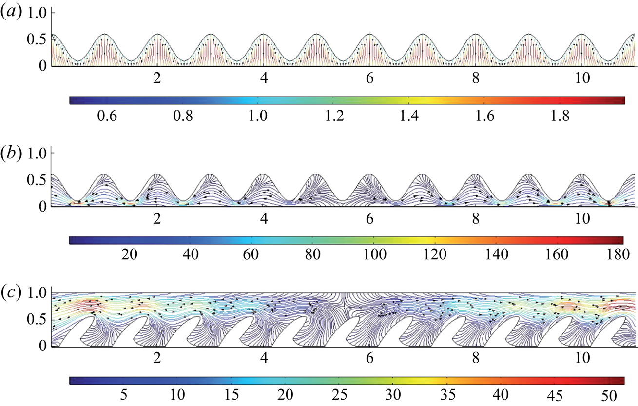
The PSNS were performed considering a channel composed of 11 geometrical unit cells, and it was verified that similar results were obtained considering larger values of  $N$. In all the simulations, the origin of the coordinate axes is located at the lower left corner of the system. The pore-scale streamlines for the three cases listed above are presented in figure 3. Regarding these results, the following comments are in order:
(i) In case a, the streamlines appear to be periodic from one geometric unit cell to another. Since
$\varphi _0^*=0$, fluid is released from the upper wall and absorbed at the lower wall at the same rate so that the net flow is directed from the upper to the lower wall and no overall flow is directed towards $\mathscr {A}_{M\beta e}$. In fact, similar results are obtained if, instead of (4.5), one imposes periodic boundary conditions at $\mathscr {A}_{M \beta e}$, which complies with mass conservation in this case.(ii) In cases b and d, there is a net fluid source, with
$\varphi _0^*>0$. Consequently, the fluid tends to move from the channel centre towards $\mathscr {A}_{M \beta e}$. Notice that, in case d, the streamlines do not follow a symmetric pattern: the velocity is larger near the left macroscopic boundary than near the right one.(iii) The results for case c are equivalent to those shown in figure 3(b), except that the maximum values are divided by a factor of 2, and they are not reported in this figure for the sake of brevity.


Pore-scale streamlines corresponding to (a) case a, (b) case b and (c) case d. Case c is not reported for the sake of brevity.

The predictions from the macroscopic model derived here are compared with these PSNS for the above four cases. Comparisons are made in terms of the horizontal and vertical components of the average velocity vector,  $\langle \boldsymbol {v}^* \rangle$, and the intrinsic average pressure,
 $\langle p^* \rangle ^\beta$. It should be noted that a straightforward consequence of the mass equation for these geometries is that the profiles of
 $\langle v_x^* \rangle$ along
 $x^*$ are linear with a slope equal to
 $\varphi _0^*$, a feature that was recovered in all the four cases with the PSNS and the macroscale predictions.
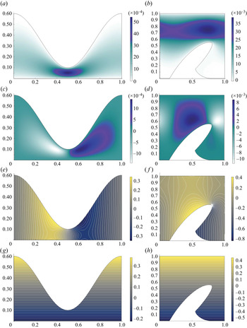
A salient feature of the upscaling approach presented in § 3 is that it is necessary to solve only one closure problem (see (3.14)) in order to compute the field of  ${\boldsymbol{\mathsf{D}}} ^*$, from which
 ${\boldsymbol{\mathsf{K}}}^*$ is obtained, and the field of
 $\boldsymbol {d}_1^*$, from which
 $\boldsymbol {v}_d^*$ can be deduced, for any source distribution. The fields of the closure variables are presented for both channel geometries in figure 4. Specifically, the fields of the
 $xx$- and
 $yx$-components of the closure tensor
 ${\boldsymbol{\mathsf{D}}}^*$ are presented in figure 4(a–d). Since the channels do not percolate in the
 $y$-direction, the
 $xy$- and
 $yy$-components of
 ${\boldsymbol{\mathsf{D}}}^*$ are zero for both geometries (see (3.19a)). In addition, the fields of the
 $x$- and
 $y$-components of the closure variable vector
 $\boldsymbol {d}_1^*$ are shown in figure 4(e–g). As expected, the fields of
 $d_{1y}^*$ in figure 4(g,h) are in agreement with (3.19b). From the solution for
 ${\boldsymbol{\mathsf{D}}}^*$, it follows that the components of the permeability tensor are
 $K_{yx}^*= K_{xy}^*=K_{yy}^* =0$ for both channels, while the only non-zero term is
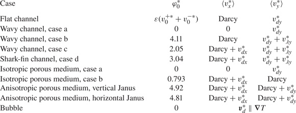
 $K_{xx}^*$. Its values are reported in table 1.
Fields of the closure variables corresponding to (a,c,e,g) the wavy channel and (b,d, f,h) the shark-fin channel: (a,b)  $D_{xx}^*$, (c,d)
 $D_{yx}^*$, (e, f)
 $d_{1x}^*$ with isolines, and (g,h)
 $d_{1y}^*$ with isolines. The fields of
 $D_{xy}^*$ and
 $D_{yy}^*$ are zero and are not represented here.

Values of the permeability ( ${\boldsymbol{\mathsf{K}}}^*$) and the components of
 $\boldsymbol {v}_s^*$ for all the numerical simulation cases. Note that
 $v_{\lambda x}^*$ was found to be irrelevant in all cases.

Under these circumstances, the equation resulting from the combination of the macroscale mass and momentum equations reduces to
 \begin{equation} K_{xx}^*\frac{\textrm{d}^2\langle p^*\rangle^\beta}{{\textrm{d}x}^{*2}} =-\varphi_0^*, \end{equation}
which is subject to the following boundary conditions:
 \begin{gather} \text{at }x^*=x_0^*, \quad \langle p^*\rangle^\beta = p_0^*, \end{gather}
 \begin{gather}\text{at }x^*=x_L^*, \quad \langle p^*\rangle^\beta = p_L^*. \end{gather}
Here,  $p_0^*$ and
 $p_L^*$ are the values of the dimensionless intrinsic average pressure obtained from the PSNS at the first and last unit cell, located at
 $x_0^*= 0.5$ and
 $x_L^*=10.5$, respectively. The analytical solution of this boundary-value problem is
 \begin{equation} \langle p^*\rangle^\beta=p_0^*+\frac{(p_L^*-p_0^*)(x^*-x_0^*)}{(x_L^*-x_0^*)}-\frac{\varphi_0^* }{2K_{xx}^*}[x^{*2}-x_0^{*2}-(x_L^*+x_0^*)(x^*-x_0^*)]. \end{equation}
From the above expression, it is easy to obtain
 \begin{equation} \frac{\textrm{d}\langle p^*\rangle^\beta}{{\textrm{d}x}^*} = \frac{(p_L^*-p_0^*)}{(x_L^*-x_0^*)} -\frac{\varphi_0^* }{2 K^*_{xx}}[2x^*-(x_L^*+x_0^*)], \end{equation}
which is further used to compute the Darcy term.
The values of the two terms  $\boldsymbol {v}_d^*$ and
 $\boldsymbol {v}_\lambda ^*$ change for each case study as reported in table 1. Nevertheless, some insight can be obtained from the results in figure 4(e). In this graph, it is observed that
 $d_{1x}^*$ is antisymmetric around
 $x^*=0.5$ at both solid–fluid interfaces. This means that the contributions from
 $v_{dx}^*$ should be zero for the wavy channel when
 $v_0^*$ is uniform at
 $\mathscr {A}_{\beta \sigma }$. However, this is not true for the shark-fin channel. In this configuration, the contributions from both
 $d_{1x}^*$ and
 $d_{1y}^*$ are relevant because no particular antisymmetry condition is observed. Furthermore, since the permeability is zero in the
 $y$-direction, it follows that
 ${v}_{sy}^*$ should be the only relevant term in the predictions of
 $\langle v_y^*\rangle$ in both channel geometries.
Regarding the predictions of  $\boldsymbol {\lambda }^*$, its values are obtained from a combination of the macroscale model and PSNS in a reduced macroscale domain. As mentioned in § 3.2, the pore-scale equations can be solved in a subdomain of
 $\mathscr {V}_M$ containing either three or five geometric unit cells in order to obtain the values of
 $\langle v_x^*\rangle$ and
 $\langle v_y^*\rangle$. These values show periodic oscillations about a geometric unit cell. Once smoothed by a second spatial average over a moving unit cell, as suggested by Barrère (Reference Barrère1990), and substituted into the macroscale momentum equations, they allow
 $\lambda _x^*$ and
 $\lambda _y^*$ to be computed. For the cases described above, it was found that
 $\lambda _x^*$ is irrelevant, i.e.
 $v_{\lambda x}^*=0$. However, the same is not true for
 $\lambda _y^*$ (
 $v_{\lambda y}^*\neq 0$). Moreover, it was noted that a subdomain made of three unit cells is sufficient, as the same value of
 $\lambda _y^*$ was obtained on the central unit cell for a subdomain made of five (or even more) unit cells.
4.1.1. Case a: wavy channel, $\varphi _0^*=0$

In this case, the macroscopic pressure is constant along the system and, therefore, the Darcy term plays no role in the prediction of  $\langle \boldsymbol {v}^* \rangle$. In addition,
 $\boldsymbol {v}_{\lambda }^*=\boldsymbol {0}$ because
 $\varphi _0^*=0$ and, since
 $v_{dx}^*=0$, as already noted,
 $\langle v_x^*\rangle =0$. Furthermore, the vertical component of the macroscale velocity is completely determined by
 $v_{dy}^*$ (see value in table 1) and, in this case, it has the value of
 $\langle v_y^*\rangle = -0.854$. These macroscopic results were checked to be in perfect agreement with those from the PSNS.
4.1.2. Case b: wavy channel, $v_0^*=1$

In this case, the mean flow goes from the centre of the system towards  $\mathscr {A}_{M\beta e}$, as shown in figure 3(b). Hence, the macroscale velocity and pressure are
 $x$-dependent along the channel. As shown in figure 5, the macroscopic variables
 $\langle p^* \rangle ^\beta$ and
 $\langle v_y^* \rangle$ obtained from PSNS exhibit an oscillatory behaviour, with a period corresponding to that of the geometrical unit cell. The PSNS profiles can be subject to a double spatial smoothing as described above in order to eliminate the spatial oscillations. These non-oscillatory results (referred to as PSNS (smoothed) in figure 5) are in excellent agreement with the predictions from the UM derived here. In this way, the macroscopic pressure follows a parabolic profile, with its maximum located at the centre of the domain that is correctly described by (4.7). The linear profile of the
 $x$-component of the macroscale velocity is in agreement with the Darcy-term contribution. For the
 $y$-component of the macroscopic velocity, the values of
 $v_{dy}^*$ and
 $v_{\lambda y} ^*$ reported in table 1 lead to
 $\langle v_y^*\rangle = -0.3$. This value matches the smoothed PSNS result, as shown in figure 5(c). From this point on, the doubly smoothed PSNS results are no longer reported for the sake of brevity in presentation.
Comparisons of the averaged results of the PSNS with the predictions from the UM for (a)  $\langle p^*\rangle ^\beta$, (b)
 $\langle v_x^*\rangle$ and (c)
 $\langle v_y^*\rangle$. These results correspond to case b for flow in a wavy channel, in which
 $v_0^*=1$ at
 $\mathscr {A}_{\beta \sigma }$.

4.1.3. Case c: wavy channel, Janus-type configuration
This case is of interest because  $v_0^*$ features a heterogeneous distribution along the channel walls. Nevertheless, as expected, the global amount of exuded fluid in this case is half that in case b, i.e.
 $\varphi _0^*= 2.05$. Results obtained from the PSNS are qualitatively equivalent to those reported in figures 3(b) and 5, all values being affected only by a coefficient
 $1/2$. In contrast to case b,
 $\langle v_x^* \rangle$ is shifted by
 $v_{dx}^*$, which is non-zero in the present case (see value in table 1) due to the uneven source distribution. As indicated in table 1,
 $v_{dy}^*$ is half the value reported for case b. In addition, the value of
 $\lambda _y^*$ was found to remain unaltered in comparison to case b, so that
 $\langle v_y^*\rangle = -0.15$, which is half the value found in case b. This is again in excellent agreement with the smoothed value obtained from the PSNS, and the same comment applies to the profiles of
 $\langle p^*\rangle ^\beta$ and
 $\langle v_x^* \rangle$. These results are not represented here for the sake of brevity in presentation.
4.1.4. Case d: shark-fin channel, $v_0^*=1$

The last channel case considered here corresponds to the shark-fin configuration with  $v_0^*=1$ throughout
 $\mathscr {A}_{\beta \sigma }$. In contrast to case b, now
 $v_{dx}^*$ is non-zero due to the non-symmetric geometry. Furthermore, taking the values of
 $v_{dy}^*$ and
 $v_{\lambda y}^*$ reported in table 1,
 $\langle v^*_y \rangle =0.725$, which, again, exactly coincides with the PSNS result as shown in figure 6(c). In the same figure, it is evident that
 $\langle p^*\rangle ^\beta$ and
 $\langle v_x^*\rangle$ are also in agreement with the PSNS results. Contrary to the previous cases,
 $\langle p^*\rangle ^\beta$ and
 $\langle v_y^*\rangle$ are not evenly distributed at the macroscopic boundaries and, interestingly, they exhibit less-pronounced oscillations along the domain than those observed in figures 5(a) and 5(c). Finally,
 $\langle v_x^*\rangle$ follows a linear profile, which is not entirely described by the Darcy term since it is shifted by
 $v_{dx}^*\neq 0$.
Comparisons of the averaged results of the PSNS with the predictions from the UM for (a)  $\langle p^*\rangle ^\beta$, (b)
 $\langle v_x^*\rangle$ and (c)
 $\langle v_y^*\rangle$. These results correspond to case d for flow in a shark-fin channel, in which
 $v_0^*=1$ at
 $\mathscr {A}_{\beta \sigma }$.

4.2. Flow in porous media
A second set of numerical experiments was performed in simple two-dimensional model porous media constructed by  $x$ and
 $y$ repetitions of a periodic unit cell with isotropic and anisotropic geometries for the solid phase. The following two types of distributions are considered for
 $v_0^*$ in the isotropic geometry.
(i) Case a: a sine-like exuding condition for which
$\varphi _0^*=0$.(ii) Case b: Janus exuding grains, which refers to a single object featuring two-sided contrasted properties, namely
$v_0^*=1$ and $v_0^*=0$ on each half-part of the grain surface.


The last  $v_0^*$ distribution is also applied in the anisotropic geometry.
4.2.1. Isotropic geometry
Consider a porous medium made up of an array of periodic unit cells in which the solid phase is modelled as a circular obstacle, as shown in figure 7. The macroscopic domain is modelled as a square of side length  $L=N\ell _{cell}$, with
 $N=11$, although similar results were observed for larger values of
 $N$. The porosity is taken equal to 0.8.
Representation of a model porous medium of characteristic length  $L$, made of an array of periodic unit cells of length
 $\ell _{cell}$. The solid phase is modelled as a circular obstacle of diameter
 $\ell _\sigma$.

4.2.1.1 Case a: sine-like exuding condition.
As a first case study, consider a situation in which  $v_0^*$ obeys the following sinusoidal function:
 \begin{equation} v_0^* = \frac{2(y^*-y^*_0)}{\ell_\sigma^*}=\sin(\theta), \quad \text{at }\mathscr{A}_{\beta\sigma}, \end{equation}
where  $\theta$ is the inclination of the position vector of a point on
 $\mathscr {A}_{\beta \sigma }$ on the horizontal axis (see figure 7). In addition,
 $y_0^*$ is the dimensionless
 $y$-coordinate of the centroid of each solid inclusion, whereas
 $\ell _\sigma ^*$ is the dimensionless diameter of the inclusion. In this way,
 $v_0^*$ is position-dependent at
 $\mathscr {A}_{\beta \sigma }$, albeit periodic. Furthermore, the boundary condition given in (4.9) leads to
 $\varphi _0^*=0$. This means that, in this case, it is physically acceptable to impose periodic boundary conditions at
 $\mathscr {A}_{M \beta e}$ instead of (4.5) without compromising conservation of mass. Hence, it is not necessary to solve the pore-scale problem in
 $\mathscr {V}_M$ made of the
 $N\times N$ unit cells; it suffices to carry out the solution in only one geometrical unit cell.
The pore-scale velocity fields are presented in figure 8 both at  $\mathscr {A}_{\beta \sigma }$ (figure 8a) and in the unit cell domain (figure 8b,c), as a result of the PSNS. The pressure fields are not reported in this figure, as they are uniformly zero. Both components of the velocity exhibit an oscillatory behaviour at
 $\mathscr {A}_{\beta \sigma }$; however,
 $v_x^*$ has cancelling amplitudes and
 $v_y^*\ge 0$. Consequently, it is not surprising that
 $\langle v_x^*\rangle =0$; in addition,
 $\langle v_y^*\rangle =0.404$.
Dimensionless pore-scale fields of (a)  $v_x^*=\sin (\theta ) \cos (\theta )$ and
 $v_y^*=\sin ^2(\theta )$ at the solid–fluid interface corresponding to the sinusoidal distribution of
 $v_0^*$, (b)
 $v_x^*$ and (c)
 $v_y^*$ in the unit cell domain.

Focusing now on the UM, the closure problem was solved in the periodic unit cell sketched in figure 7. The resulting fields of the closure variables are represented in figure 9. Clearly, the diagonal components of tensor  ${\boldsymbol{\mathsf{D}}}^*$ are
 $x$- and
 $y$-symmetric fields, whereas the off-diagonal components are antisymmetric. As a consequence,
 ${\boldsymbol{\mathsf{K}}}^*$ is a spherical tensor, i.e.
 ${\boldsymbol{\mathsf{K}}} ^*=K^*{\boldsymbol{\mathsf{I}}}$, and the value of
 $K^*$ is reported in table 1.
Fields of the closure variables (a)  $D_{xx}^*$, (b)
 $D_{yx}^*$, (c)
 $D_{xy}^*$, (d)
 $D_{yy}^*$, (e)
 $d_{1x}^*$ and ( f)
 $d_{1y}^*$ in the periodic unit cell sketched in figure 7 for a porosity value of 0.8.

Regarding the fields of the closure vector  $\boldsymbol {d}_1^*$, the results for the
 $x$- and
 $y$-components are represented in figures 9(e) and 9( f), showing that
 $d_{1x}$ and
 $d_{1y}$ are antisymmetric about the vertical and horizontal directions, respectively. It is worth recalling that these results are intrinsic to the geometry, i.e. they are independent of
 $v_0^*$. In addition, since there is no macroscopic pressure gradient in any direction, it follows that the Darcy term in the macroscale momentum equation (3.20b) is zero, thus simplifying the model to
 $\langle \boldsymbol {v}^*\rangle =\boldsymbol {v}_s^*$. Finally, since
 $\varphi _0^*=0$ in this case,
 $\boldsymbol {v}_\lambda ^*=\boldsymbol {0}$ and
 $\boldsymbol {v}_s^*=\boldsymbol {v}_d^*$. With the values reported in table 1, this leads to a perfect match with the PSNS data.
4.2.1.2 Case b: Janus exuding grains.
The second case study deals with a Janus-type configuration for  $v_0^*$, such that
 \begin{equation} v_0^* = \begin{cases} 1 & \text{when} \ 0<\theta <{\rm \pi}/2\ \text{and} \ 3{\rm \pi}/2 < \theta < 2{\rm \pi},\\ 0 & \text{when} \ {\rm \pi}/2 <\theta < 3{\rm \pi}/2. \end{cases} \end{equation}
Solving the governing equations at the pore scale subject to the macroscopic boundary condition provided in (4.5) gives rise to the velocity and pressure fields reported in figure 10. The field of  $v_x^*$ is
 $y$-symmetric but not
 $x$-symmetric, whereas the field of
 $v_y^*$ is
 $x$-symmetric and
 $y$-antisymmetric. The pressure field is
 $x$- and
 $y$-symmetric, with a maximum value located at the centre of the domain.
Fields of (a)  $v_x^*$, (b)
 $v_y^*$ and (c)
 $p^*$ obtained from pore-scale numerical simulations considering the Janus exuding grains.

These observations suggest that the solution of the governing macroscale pressure differential equation
 \begin{equation} \nabla^{*2} \langle p^*\rangle^\beta = -\frac{\varphi_0^* }{K^*} \end{equation}
can be performed in one quarter of the macroscopic domain. Note that, in the above equation, the isotropic nature of the permeability tensor was taken into account. Locating the origin of the coordinate axes at the macroscopic domain centre, the solution of (4.11a) is subject to the following set of boundary conditions:
 \begin{gather} \text{at } x^*=0, \quad \frac{\partial \langle p^*\rangle^\beta}{\partial x^*} =0, \end{gather}
 \begin{gather}\text{at } y^*=0, \quad \frac{\partial \langle p^*\rangle^\beta}{\partial y^*} =0, \end{gather}
 \begin{gather}\text{at } x^*=x_L^*, \quad \langle p^*\rangle^\beta =p_{Lx}^*(y^*), \end{gather}
 \begin{gather}\text{at } y^*=y_L^*, \quad \langle p^*\rangle^\beta =p_{Ly}^*(x^*). \end{gather}
The first two boundary conditions follow from the macroscale pressure-field symmetries. As in the analysis of the corrugated channels,  $x_L^*$ and
 $y_L^*$ locate the positions of the last centroids of the unit cells where the PSNS data were collected (i.e.
 $x^*=y^*=5$). Hence, the functions
 $p_{Lx}^*(y^*)$ and
 $p_{Ly}^*(x^*)$ are extracted from the PSNS.
Owing to the  $y$-antisymmetry of
 $d_{1y}^*$ exhibited in figure 9( f), it follows that
 $v_{dy}^*=0$. With the data reported in table 1 for
 $v_{dx}^*$ and
 $\varphi _0^*$, it is possible to carry out the UM solution and compute the profiles of the macroscale velocity and pressure. These results are reported in figure 11 and they are compared with those arising from the average PSNS data for various values of
 $y^*$. The simulations from the UM are found to be in good agreement with the PSNS without requiring the computation of
 $\boldsymbol {v}_\lambda ^*$. In order to appreciate the relevance of
 $\boldsymbol {v}_d^*$, the predictions of
 $\langle v_x^*\rangle$, considering only the Darcy term, are compared with the PSNS results in figure 11(b), showing a clear discrepancy. The two sets of curves differ by a constant vertical shift, corresponding to
 $v_{dx}^*$. It should be noted that the magnitude of the macroscopic pressure gradient builds up while moving away from the centre of the domain, thus increasing
 $\langle v_x^* \rangle$. Consequently, since
 $\boldsymbol {v}_d^*$ is a constant vector, its relative contribution decreases when the Darcy term becomes dominant.
Comparison of the macroscopic velocity (a–c) and pressure (d) profiles obtained from the UM and PSNS for the Janus exuding grains. In (b), the horizontal averaged velocity results from PSNS are compared with those from Darcy's law.

When considering the results for  $\langle v_y^* \rangle$ and
 $\langle p^* \rangle ^\beta$ represented in figures 11(c) and 11(d), respectively, it is observed that the averaged PSNS results follow an oscillatory behaviour, more prominent for
 $\langle v_y^*\rangle$. Nevertheless, the predictions from the UM are in excellent agreement with the PSNS results once doubly smoothed for all the values of
 $y^*$ considered here.
4.2.2. Anisotropic geometry
A further illustration may now be considered consisting of flow in an anisotropic medium with porosity  $\varepsilon =0.621$, constructed by an
 $N\times N$ repetition in the
 $x$- and
 $y$-directions (
 $N=11$ in the present case) of the periodic unit cell shown in figure 12. For this case,
 $v_0^*=1$ at the blue shaded part of
 $\mathscr {A}_{\beta \sigma }$ shown in this figure, while
 $v_0^*=0$ at the remaining part of the solid–fluid interfaces. This arrangement is referred to as a vertical Janus configuration in the following paragraphs. Imposing the boundary condition given in (4.5) at
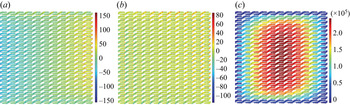
 $\mathscr {A}_{M \beta e}$, and carrying out PSNS, yields the velocity and pressure fields shown in figure 13. The numerical results are somewhat similar to those presented in figure 11 in the sense that the fluid tends to move from the centre towards the macroscopic boundaries.
Periodic unit cell used to construct the anisotropic porous medium. The boundaries at which  $v_0^*$ is set to one are shaded in blue.

Pore-scale fields of (a)  $v_x^*$, (b)
 $v_y^*$ and (c)
 $p^*$ obtained from the vertical Janus configuration in the anisotropic geometry.

The fields of all the closure variables, obtained after solving the closure problem in the geometric unit cell shown in figure 12, are represented in figure 14. Clearly, no symmetric or antisymmetric property is observed. From this solution, the components of the permeability tensor, which is now a full matrix, can be computed and the results are reported in table 1 along with the values of  $\varphi _0^*$,
 ${v}_{dx}^*$ and
 ${v}_{dy}^*$.
Fields of the closure variables (a)  $D_{xx}^*$, (b)
 $D_{yx}^*$, (c)
 $D_{xy}^*$, (d)
 $D_{yy}^*$, (e)
 $d_x^*$ and ( f)
 $d_y^*$ for the anisotropic geometry.

Since no symmetry properties are applicable to the pressure, the UM must be solved in the entire macroscopic domain,  $\mathscr {V}_M$. Locating the origin of the coordinate axes at the system centre, the macroscale pressure solves the following boundary-value problem:
 \begin{gather} {\boldsymbol{\mathsf{K}}}^* \boldsymbol{:} \boldsymbol{\nabla}^*\boldsymbol{\nabla}^* \langle p^*\rangle^\beta = -\varphi_0^*, \end{gather}
 \begin{gather}\text{at } x^*=-x_L^*, \quad \langle p^*\rangle^\beta = p_{0x}^*(y^*), \end{gather}
 \begin{gather}\text{at } x^*=x_L^*, \quad \langle p^*\rangle^\beta = p_{Lx}^*(y^*), \end{gather}
 \begin{gather}\text{at } y^*=-y_L^*, \quad \langle p^*\rangle^\beta = p_{0y}^*(x^*), \end{gather}
 \begin{gather}\text{at } y^*=y_L^*, \quad \langle p^*\rangle^\beta = p_{Ly}^*(x^*). \end{gather}
As in the previous case,  $x_L^*=y_L^*=5$, while
 $p_{0i}^*$ and
 $p_{Li}^*$ (
 $i=x,y$) are functions of position that are obtained from the PSNS. Despite the fact that this problem was solved in the entire domain, the comparisons with the PSNS data are reported in figure 15 for only one quarter of
 $\mathscr {V}_M$ for the sake of brevity in presentation. The macroscale velocity and pressure profiles barely change for
 $y^*=0$, 1 and 2, and, for this reason, the results corresponding to
 $y^*=1$ and
 $y^*=2$ are not reported in this figure. These results are in excellent agreement with the predictions from the UM without considering the contribution from
 $\boldsymbol {v}_\lambda ^*$. Note that, as in case a for the isotropic porous medium, the relative importance of
 $\boldsymbol {v}_d^*$ with respect to the
 $\langle \boldsymbol {v}^* \rangle$ decreases while moving away from the centre of the domain.
Comparison of the macroscopic velocity (a,b) and pressure (c) obtained from the UM and the PSNS for the vertical Janus configuration in the anisotropic medium.

Finally, it is worth considering another distribution of  $v_0^*$ in the same porous medium, which can be viewed as a horizontal Janus exuding pattern. As for the vertical Janus distribution of
 $v_0^*$, an excellent agreement is found between the averaged PSNS results and the solution of the UM, without taking into account
 $\boldsymbol {v}_\lambda ^*$, which is again irrelevant in that case. The values of
 $\varphi _0^*$ and
 $\boldsymbol {v}_d^*$ are given in table 1. Most interestingly, if the contribution from
 $\boldsymbol {v}_s^*$ is neglected and if the results are normalized by
 $\varphi _0^*$, then the macroscale velocity and pressure profiles from the vertical Janus match those from the horizontal Janus. This is expected, since, when the net volume sources and outer boundary conditions are identical, the macroscopic model (3.20) predicts that the velocity fields differ only by the value of
 $\boldsymbol {v}_s^*$ associated with a particular distribution of the interfacial sources. This is a relevant result, which may be of interest in practical situations in which one may only account for
 $\varphi _0^*$ at the macroscale.
4.3. Migration of water vapour bubbles in ice
To conclude this section, an extension of this work to the migration of water vapour bubbles in ice is briefly discussed. To this end, consider an ice mass containing a dilute population of spherical bubbles. For simplicity, assume that the bubbles contain pure water vapour, so that internal mass transfer does not involve diffusion. Each bubble is assumed to be in global equilibrium, i.e. its internal pressure is equal to the saturation pressure at the temperature of the surrounding ice and its volume is constant. Any deviation would result in a net ice sublimation or vapour condensation rate, with pressure and volume variations, until an equilibrium state is reached ultimately.
Despite the global equilibrium, an overall temperature gradient can exist in the ice mass, as occurs in glaciers or polar ice caps (Mellor Reference Mellor1960). The resulting slight temperature difference across the bubble causes sublimation to take place at the warm part of its surface, and condensation on the opposite cold side. This, in turn, induces a migration of the bubble in the direction of increasing temperature. Under a quasi-steady approximation, it is reasonable to neglect interfacial displacement, so that the transfers at a bubble boundary correspond to
 \begin{equation} v_0^*= \frac{\rho_i}{\rho_v} \boldsymbol{n}\boldsymbol{\cdot} \underbrace{\left(\frac{3 k_i}{\rho_i L_s v_{ref}} \boldsymbol{\nabla} T \right)}_{\boldsymbol{v}_B^*}, \quad \text{at }\mathscr{A}_{\beta\sigma}. \end{equation}
Here  $\rho _i$ and
 $\rho _v$ denote the densities of ice and water vapour, respectively. In addition,
 $k_i$ is the thermal conductivity of the ice,
 $L_s$ is the latent heat of sublimation and
 $\boldsymbol {\nabla } T$ is the overall temperature gradient. Finally, the term in parentheses in the above equation corresponds to the dimensionless bubble velocity,
 $\boldsymbol {v}_B^*$. Its expression results from an energy balance, and shows that it does not depend on the bubble size (Shreve Reference Shreve1967). The source distribution in (4.13) results in
 $\varphi _0^*=0$, in agreement with the global equilibrium hypothesis.
A simple way to derive an expression for the macroscopic vapour velocity, without actually solving the flow problem, is by noticing that  $\boldsymbol {v}^*=\boldsymbol {\nabla }^*\boldsymbol {\cdot }(\boldsymbol {v}^*\boldsymbol {r}^*)$ and applying the intrinsic averaging operator together with the divergence theorem to obtain
 \begin{equation} \langle \boldsymbol{v}^*\rangle^\beta = -\frac{1}{V_\beta^*}\int_{\mathscr{A}_{\beta\sigma}} v_0^* \boldsymbol{r}^*\,\textrm{d}A^* = -\frac{\rho_i}{\rho_v} \boldsymbol{v}_B^*. \end{equation}
The last equality results from substitution of  $v_0^*$ from (4.13) in the integral. In fact, this interfacial integral can be identified as the source dipole. For instance, if the source and sinks were concentrated at two points, it would reduce to a usual point-source dipole (Pozrikidis Reference Pozrikidis2003; Spagnolie & Lauga Reference Spagnolie and Lauga2012).
Since the pore space in the ice is made of disconnected cavities, its permeability coefficient is zero, hence the Darcy term in (3.16) vanishes and the macroscopic velocity reduces to  $\langle \boldsymbol {v}^*\rangle =\boldsymbol {v}_s^*=\boldsymbol {v}_d^*$ because
 $\varphi _0^*=0$. In this way, the closure problem given in (3.14) can be solved in a unit cell containing a single bubble. It is readily apparent that
 ${\boldsymbol{\mathsf{D}}}^*=\boldsymbol {0}$ (and therefore
 ${\boldsymbol{\mathsf{K}}}^*=\boldsymbol {0}$) and
 $\boldsymbol {d}_1^*=\boldsymbol {r}^*-\boldsymbol {r}_G^*$ as mentioned in § 3.2 (see (3.19)). Substitution of this result into (3.17), along with the expression for
 $v_0^*$ given in (4.13), taking into account the fact that
 $\varphi _0^*=0$, leads to an expression for
 $\langle \boldsymbol {v}^*\rangle$, which, when divided by the porosity, allows the result given in (4.14) to be recovered. This can be straightforwardly extended to periodic media where the unit cell contains any number of bubbles, possibly with different sizes. Thus, the UM established in the previous section accommodates this peculiar situation of a non-percolating porous medium, and predicts the correct mean gas velocity.
To summarise the different situations investigated with the above examples, the features of the macroscopic velocity components are reported in table 2, highlighting the richness of the problem. Note that the Darcy model is applicable in the minority of the cases studied here. When  $\varphi _0^*=0$, there is no Darcy term in the macroscale model.
Summary of the macroscopic velocity features in the different case studies. The values of  $v_{dx}^*$,
 $v_{dy}^*$ and
 $v_{\lambda y}^*$ are reported in table 1. In the last two columns, the term ‘Darcy’ denotes the projection of
 $-{\boldsymbol{\mathsf{K}}}^*\boldsymbol {\cdot } \boldsymbol {\nabla }^*\langle p^*\rangle ^\beta$ on the corresponding direction.

5. Discussion and conclusions
In this work, a macroscale model describing incompressible, Newtonian and creeping flow in exuding rigid and homogeneous porous media was derived. The governing transport equations at the pore scale correspond to those involved in the derivation of Darcy's law, with the difference that a normal mass flux is present at the solid–fluid interface. Despite the apparent simplicity of this problem, this physical situation is quite rich. Indeed, mass conservation prevents, in general, the simplification of the problem to a single periodic unit cell. Therefore, the use of periodic boundary conditions in the course of the upscaling process must be treated with caution. Nevertheless, a common practice in the literature is to use the classical Darcy's law at the macroscopic level, which raises the question about the pertinence of such an equation and/or whether or not the permeability tensor can remain intrinsic.
The upscaling of the governing pore-scale equations developed in this work contrasts to the Darcy model in two respects. First, the macroscopic velocity field is non-solenoidal. The non-solenoidal nature of the average velocity (despite the fact that the flow is incompressible) is a relevant modification to the classical Darcy model, albeit not the only one, as it accounts for the mass entering or exiting the system through the solid–fluid interface. Second, the macroscale momentum equation involves the classical Darcy term (with the intrinsic permeability) and a correction term. The correction term,  $\boldsymbol {v}_s$, in the macroscopic momentum equation is the sum of a contribution,
 $\boldsymbol {v}_d$, due to the local effect of
 $v_0$ and a term,
 $\boldsymbol {v}_\lambda$, that compensates for the periodicity assumption. The magnitudes of both
 $\boldsymbol {v}_d$ and
 $\boldsymbol {v}_\lambda$ were found to be, at most, of the order of
 $v_0$. Since
 $\boldsymbol {v}_s$ is a vector, the correction only applies in one spatial direction. This can only occur if the system features privileged directions resulting from geometrical and/or
 $v_0$ distribution anisotropy. A salient feature of the model derived here is that a unique intrinsic closure problem, exactly corresponding to that involved in the classical Darcy case, is required to predict both the intrinsic permeability tensor and
 $\boldsymbol {v}_d$. The correction term,
 $\boldsymbol {v}_s$, accounts for the local fluid displacement induced by the exuding phenomenon at the solid–fluid interfaces. This effect is not captured by the Darcy term, which only accounts for the macroscopic drag. This correction term,
 $\boldsymbol {v}_s$, identifies as the average of a contribution to the flow field that does not induce any macroscopic force on the solid skeleton of the porous material.
The performance of the UM was validated in a variety of physical situations ranging from flow in flat and corrugated channels to isotropic and anisotropic porous media. For channels, the component along the channel axis of the correction term in the macroscopic momentum equation results from a complex interplay of the distribution of  $v_0$ and the geometry of the walls. This component is zero in the case of the plane channel (it can be shown that this result holds whatever
 $v_0$) or in the sine channel when
 $v_0$ is uniform. In more complex cases, a correction is needed in the axial direction and it can only be obtained from the solution of the adjoint problem. The different channel examples illustrate the pertinence of the correction in various flow situations; a detailed analysis of the role played by the topology and
 $v_0$ distribution is out of the scope of this work.
The macroscale model solution requires physically sound boundary conditions at the macroscopic boundaries. In this work, they were obtained by fitting data from the pore-scale numerical simulations at the macroscopic boundaries. Certainly, it is tempting to impose heuristic boundary conditions, such as  $\langle p\rangle ^\beta =0$ at
 $\mathscr {A}_{M\beta e}$. However, it was verified that using this approach leads to relative percentage errors larger than 10 %, especially near the macroscopic boundaries. In contrast, the approach used here leads to an error below 1 %. Certainly, this issue requires further analysis, since the derivation of macroscopic boundary conditions is still a developing research subject not specific to the exuding problem investigated here.
For the cases in which  $\varphi _0=0$ (plane channel when
 $\varphi _0=0$, wavy channel case a, isotropic porous medium case a, and bubbles in ice), periodicity is physically justified and the macroscopic model is exact to within the approximation associated with the classical length scale constraint. Since no macroscopic pressure gradient is present, it follows that a Darcy-type model is incapable of predicting the constant velocity. This result is accurately predicted by
 $\boldsymbol {v}_d$ with
 $\boldsymbol {v}_\lambda =\boldsymbol {0}$.
When the distribution of  $v_0$ is such that
 $\varphi _0\ne 0$, many different situations can occur. The pertinence of the constant correction term
 $\boldsymbol {v}_d$ with respect to the Darcy term is particular to each application. Moreover, the correction term
 $\boldsymbol {v}_\lambda$ was found to be generally irrelevant for the cases studied here. The exception is in the corrugated channel cases, for which
 $\boldsymbol {v}_\lambda$ plays a role in the non-percolating direction of the channel.
The above indicates that a Darcy-type model may be pertinent whenever the pressure gradient spatially develops so that the Darcy term overcomes the contribution from  $\boldsymbol {v}_s$. Nevertheless, it should be noted that, even if a Darcy model were to provide acceptable predictions of the macroscopic velocity, in some particular situations,
 $\boldsymbol {v}_s$ may not be neglected (see table 2). Indeed, it can trigger some mechanisms, like instability for instance, if flow is coupled to another nonlinear phenomenon, which may be overlooked if a pure Darcy model is employed.
As a matter of perspective, the combination of the UM from this work with species and/or heat transport models can be used to predict an ample variety of transport processes in porous media involving internal flow sources, such as mineral dissolution in rough fractures, as recently studied by Rasoulzadeh et al. (Reference Rasoulzadeh, Yekta, Deng and Ghahfarokhi2020). Finally, the results from this work should also call for complementary experimental investigation.
Acknowledgements
D.L. and F.J.V.-P. wish to thank A. Bottaro (University of Genoa) for insightful discussions.
Funding
D.L. would like to gratefully acknowledge support from UAM (CDMX) in November 2018 and 2019, periods during which part of this work was completed. F.J.V.-P. would like to thank the CNRS for the support for a one-month stay at I2M during 2019.
Declaration of interests
The authors report no conflict of interest.
Appendix A. Order-of-magnitude estimates
The purpose of this appendix is to provide order-of-magnitude estimates for the correction vectors  $\boldsymbol {v}_d$ and
 $\boldsymbol {v}_\lambda$. To this end, it is convenient to commence the analysis by examining the boundary-value problem given in equations (3.3), which are subject to homogeneous boundary conditions at
 $\mathscr {A}_{\beta e}$. This means that this problem is driven by the unitary volume source in (3.3b). From this observation, the following order-of-magnitude estimate can be made
 \begin{equation} \boldsymbol{d} = {O}(\ell_\beta). \end{equation}
Since  $\boldsymbol {\lambda }=\langle \boldsymbol {d}\rangle ^\beta$, it follows that
 $\boldsymbol {\lambda }= {O}(\ell _\beta )$, with the idea that this represents an upper bound. Directing attention to the closure problem defined in (3.14), a similar analysis leads to the estimate
 \begin{equation} \boldsymbol{d}_1 = {O}(\ell_\beta). \end{equation}
Taking these results into account, the order-of-magnitude estimates for  $\boldsymbol {v}_d$ and
 $\boldsymbol {v}_\lambda$ are derived as
 \begin{gather} \boldsymbol{v}_d = -\frac{1}{V}\int_{\mathscr{A}_{\beta\sigma}} v_0 \boldsymbol{d}_1\,\textrm{d}A = {O}( v_0 ), \end{gather}
 \begin{gather}\boldsymbol{v}_\lambda = -\boldsymbol{\lambda} \varphi_0 = {O}( v_0 ), \end{gather}
which are again upper bounds. With these results, it immediately follows that  $\boldsymbol {v}_s = {O}(v_0)$ and this concludes the derivations.