1 Introduction
The non-equilibrium thermokinetic problem (in a liquid) that includes electrokinetic phenomena usually becomes an extremely challenging problem. What makes the problem difficult? One major reason is the lack of a cross-sectional integrated physical concept, even excepting the fact that non-equilibrium thermodynamics has not yet been completely established, although many challenging works have been devoted to this purpose (Würger Reference Würger2010). The thermokinetic phenomena have been known as the Soret effect since the nineteenth century and they are recognized as important phenomena, which can be used for various biomedical applications, such as efficient separation techniques for macro-molecules (Giddings Reference Giddings1993) and a molecular trap for DNA (Duhr & Braun Reference Duhr and Braun2006a
). That is, under the existence of a temperature gradient
 $\unicode[STIX]{x1D735}T$
, the thermal drift velocity is described as
 $$\begin{eqnarray}\boldsymbol{u}=-D_{T}\unicode[STIX]{x1D735}T\end{eqnarray}$$
based on Onsager’s reciprocal theorem with the definition of a Soret coefficient
 $$\begin{eqnarray}S_{T}\equiv D_{T}/D,\end{eqnarray}$$
where
 $D$
is the ordinary diffusion coefficient of Einstein and
 $D_{T}$
is the thermodiffusion coefficient. Here,
 $D_{T}$
and
 $S_{T}$
are generally considered just as phenomenological parameters determined by experiments in spite of many theoretical efforts; i.e. the generally accepted complete theory that accounts for the puzzling behaviours of
 $D_{T}$
(or
 $S_{T}$
) for all situations does not exist and many unsolved problems remain in this field (Würger Reference Würger2007, Reference Würger2008, Reference Würger2010; Eslamian & Saghir Reference Eslamian and Saghir2009; Huang et al.
Reference Huang, Lundstrom, Holmden, Glessner, Kieffer and Lesher2010). Note that difficulty exists in the remarkable sensitivity of
 $S_{T}$
(and
 $D_{T}$
) to many factors (Huang et al.
Reference Huang, Lundstrom, Holmden, Glessner, Kieffer and Lesher2010), e.g. size (Duhr & Braun Reference Duhr and Braun2006b
) and temperature (Putnam, Cahill & Wong Reference Putnam, Cahill and Wong2007). This is why this field is challenging.
It is natural to consider the extended Nernst–Plank (NP) equations that consider the thermokinetic term using an Eastman entropy transfer
 $Q^{\ast }/T$
(Eastman Reference Eastman1926, Reference Eastman1928) as a fundamental equation at least for a colloidal particle that has an electric double layer, where
 $Q^{\ast }$
is a ionic heat of transfer which is studied extensively by Agar, Mou & Long Lin (Reference Agar, Mou and Long Lin1989). Further, although researchers in the field of thermokinetics often neglect the electrokinetic term, some researchers have pointed out the importance of the electrokinetic term, an effect that has long been recognized as the thermoelectric effect by Guthrie, Wilson & Schomaker (Reference Guthrie, Wilson and Schomaker1949), Putnam et al. (Reference Putnam, Cahill and Wong2007) and Würger (Reference Würger2010). For example, Guthrie et al. (Reference Guthrie, Wilson and Schomaker1949) succeeded in explaining the anomalous difference between the thermal diffusion coefficient of an ion in the presence and in the absence of another electrolyte based on an equation that considers molecular diffusion, thermal diffusion and electrophoretic terms (Guthrie et al.
Reference Guthrie, Wilson and Schomaker1949). Putnam & Cahill (Reference Putnam and Cahill2005) showed that
 $D_{T}$
of charged latex spheres in aqueous suspensions is controlled by the Seebeck coefficient of the electrolyte (
 $S_{e}$
). Würger (Reference Würger2008) showed that
 $D_{T}$
of charged colloids is determined by the thermoelectric effect to a large extent by using explicitly the extended NP equation that comprises a thermodiffusion term described by the Eastman entropy as a fundamental equation for the system. Furthermore, Majee & Würger (Reference Majee and Würger2012) predicted charging phenomena of heated colloidal particles based on the extended NP equation along with the electrolyte or fluidic Seebeck effect. Thus, in this paper, we also use the extended NP equation as the fundamental equation toward a step to a general design base that bridges both electrokinetic and thermokinetic studies.
The study of the fluidic Seebeck effect is usually based on the extended NP equation (Agar et al.
Reference Agar, Mou and Long Lin1989; Bonetti et al.
Reference Bonetti, Nakamae, Roger and Guenoun2011; Majee & Würger Reference Majee and Würger2012); i.e. the fluidic Seebeck effect is defined as a thermoelectric effect that occurs in a liquid and it is often characterized by the Seebeck coefficient
 $S_{e}$
derived by the zero current condition for the extended NP equation (Würger Reference Würger2008; Bonetti et al.
Reference Bonetti, Nakamae, Roger and Guenoun2011; Majee & Würger Reference Majee and Würger2012). The fluidic Seebeck effect has also attracted much attention because of the potential for an innovative thermogalvanic cell. For example, Bonetti et al. (Reference Bonetti, Nakamae, Roger and Guenoun2011) showed a huge Seebeck effect in a non-aqueous electrolyte. Hu et al. (Reference Hu, Cola, Haram, Barisci, Lee, Stoughton, Wallace, Too, Thomas, Gestos, dela Cruz, Ferraris, Zakhidov and Baughman2010) demonstrated a high-performance thermogalvanic cell using a carbon nanotube. However, the importance of the boundary conditions and the distribution of ions have been just recently recognized and investigated by Chikina, Shikin & Varlamov (Reference Chikina, Shikin and Varlamov2012, Reference Chikina, Shikin and Varlamov2015), in a pioneering work. Thus, extensive research for the thermokinetic boundary conditions is desirable.
Just recently, a metal capped insulating particle called a Janus particle has attracted much attention from the viewpoint of a self-propulsion mechanism and possible applications such as microswimmers and nanomachines. For example, Jiang, Yoshinaga & Sano (Reference Jiang, Yoshinaga and Sano2010) experimentally showed that a Janus particle irradiated by a laser can move in the direction of the dielectric end in water by thermophoresis due to the local temperature gradient in a particle. Bickel, Majee & Würger (Reference Bickel, Majee and Würger2013) theoretically showed the flow around a metal capped Janus particle by assuming a thermophoretic surface-slip velocity proportional to the temperature gradient. However, the polarizable characteristics of a self-propelled Janus particle have not yet been considered in spite of its importance. In particular, the experimental thermokinetic velocity of a self-propelled Janus particle
 $u_{J}$
(Jiang et al.
Reference Jiang, Yoshinaga and Sano2010) is not proportional to
 $\unicode[STIX]{x1D735}T$
globally in the sense that the line of the dependence (
 $u_{J}$
versus
 $\unicode[STIX]{x1D735}T$
) does not go through the zero point. Thus, the thermokinetic phenomena in the vicinity of a polarizable material should be explored.
The electrokinetic phenomena in the vicinity of a polarizable material such as a metal particle and an electrode have only recently been recognized (Ramos et al.
Reference Ramos, Morgan, Green and Castellanos1999, Reference Ramos, Gonzalez, Castellanos, Green and Morgan2003; Bazant & Squires Reference Bazant and Squires2004; Bazant et al.
Reference Bazant, Kilic, Storey and Ajdari2009) and this new knowledge forces us to reconsider many fundamental issues on surface science in electrolytes with the expectation of tremendous microfluidic applications (Squires Reference Squires2009; Sugioka Reference Sugioka2015b
), although the study of electrokinetic phenomena is often considered to be mature. Namely, an electrokinetic vortex flow due to the interaction between a charge in an electric double layer and a tangential electric field near the surface of planar electrodes was first recognized as AC electroosmosis (ACEO) in 1999 (Ramos et al.
Reference Ramos, Morgan, Green and Castellanos1999). Immediately, these phenomena were recognized as more general phenomena near a polarizable material and termed induced-charge electroosmosis (ICEO) in 2004 (Bazant & Squires Reference Bazant and Squires2004). Here, ICEO includes ACEO and it results from the general interaction between the electric field and charges in the electric double layer formed by the polarizing effect. In particular, ICEO is typically observed as a quadrupolar vortex flow around the conductive cylinder in an electrolyte subject to an external electric field and it is characterized by a flow velocity proportional to the square of the applied electric field; i.e. ICEO is a nonlinear electrokinetic phenomenon. Various microfluidic applications such as pumps, valves, mixers, self-propelled Janus particles (a particle containing metallic and insulating surfaces), etc. (Bazant & Squires Reference Bazant and Squires2004; Sugioka Reference Sugioka2010, Reference Sugioka2015a
) have been proposed because of the large flow velocity (
 ${\sim}1~\text{mm}~\text{s}^{-1}$
) at small voltages (
 ${\sim}1$
V) examined experimentally (Urbanski et al.
Reference Urbanski, Thorsen, Levian and Bazant2006; Gangwal et al.
Reference Gangwal, Cayre, Bazant and Velev2008; Pascall & Squires Reference Pascall and Squires2010) in this decade; these have attracted much attention as promising leading-edge technologies in microfluidics. However, even now, the characteristics of ICEO have not been clarified completely and a challenging study trying to establish a design base for ICEO devices has been continued extensively (Bazant et al.
Reference Bazant, Kilic, Storey and Ajdari2009; Squires Reference Squires2009; Sugioka Reference Sugioka2015b
, Reference Sugioka2016). In particular, ICEO under the existence of a temperature gradient has not been discussed well except in our previous study (Sugioka Reference Sugioka2014b
), although a large temperature gradient often exists in microfluidic systems because of the heat flow from the electric integrated circuit of the driver or the use of heating devices in a channel. Thus, the study of ICEO under a large temperature gradient is important.
In the previous study (Sugioka Reference Sugioka2014b
), we proposed a novel mechanism to produce nonlinear thermokinetic phenomena around a metal cylinder under a large temperature gradient on the basis of analytical discussion. The most characteristic aspect of the nonlinear thermokinetic phenomena is the generation of quadrupolar vortex flows, for which the flow velocity is proportional to the square of the temperature gradient (i.e.
 $|\boldsymbol{u}|\propto (\unicode[STIX]{x1D735}T)^{2}$
), and a Janus particle, using this phenomenon, can move to both hotter and colder regions in a temperature gradient by changing the direction of its dielectric end (Sugioka Reference Sugioka2014b
). However, since nonlinear thermokinetic phenomena are very complex phenomena related to the fluidic Seebeck effect and ICEO, the details of the nonlinear thermokinetic phenomenon (NTKP) have not yet been explored. In particular, the non-steady behaviour of ions near metals under a large temperature gradient has not yet been explored, although a pioneering study on the linear thermokinetic phenomena in metals exists (Giddings, Shinude & Semenov Reference Giddings, Shinude and Semenov1995). On the other hand, several groups (Gregersen et al.
Reference Gregersen, Andersen, Soni, Meinhart and Bruus2009; Davidson, Andersen & Mani Reference Davidson, Andersen and Mani2014; Sugioka Reference Sugioka2014a
, Reference Sugioka2016) have developed direct calculation methods that calculate ICEO flows directly based on the governing equations without using a thin double layer approximation, although the direct calculation method that can calculate both the fluidic Seebeck effect and ICEO has not yet been reported to the best of the author’s knowledge.
Therefore, in this paper, we focus on non-steady direct simulation around a metal cylinder under the large temperature gradient and fundamentally clarify the nonlinear thermokinetic phenomena due to the thermoelectric effect and ICEO. In particular, by using the two-dimensional (2-D) non-steady direct simulation technique that considers the modified Nernst–Planck (NP) equation that comprises a thermophoretic diffusion term with the Stokes and Poisson equations, we will show that the quadrupolar vortex flows due to the nonlinear thermokinetic phenomena are naturally generated and become the steady state.
This paper is presented in five sections. In § 2, we describe the theories for a geometry model, a primitive mechanism, a numerical method, the dimensionless formulations, the considered modes and the simple analytical model. Based on these theories, the results for the basic non-steady analysis for various modes are presented in § 3. Following a discussion in § 4, our conclusions are summarized in § 5.
2 Theory
2.1 Geometry model
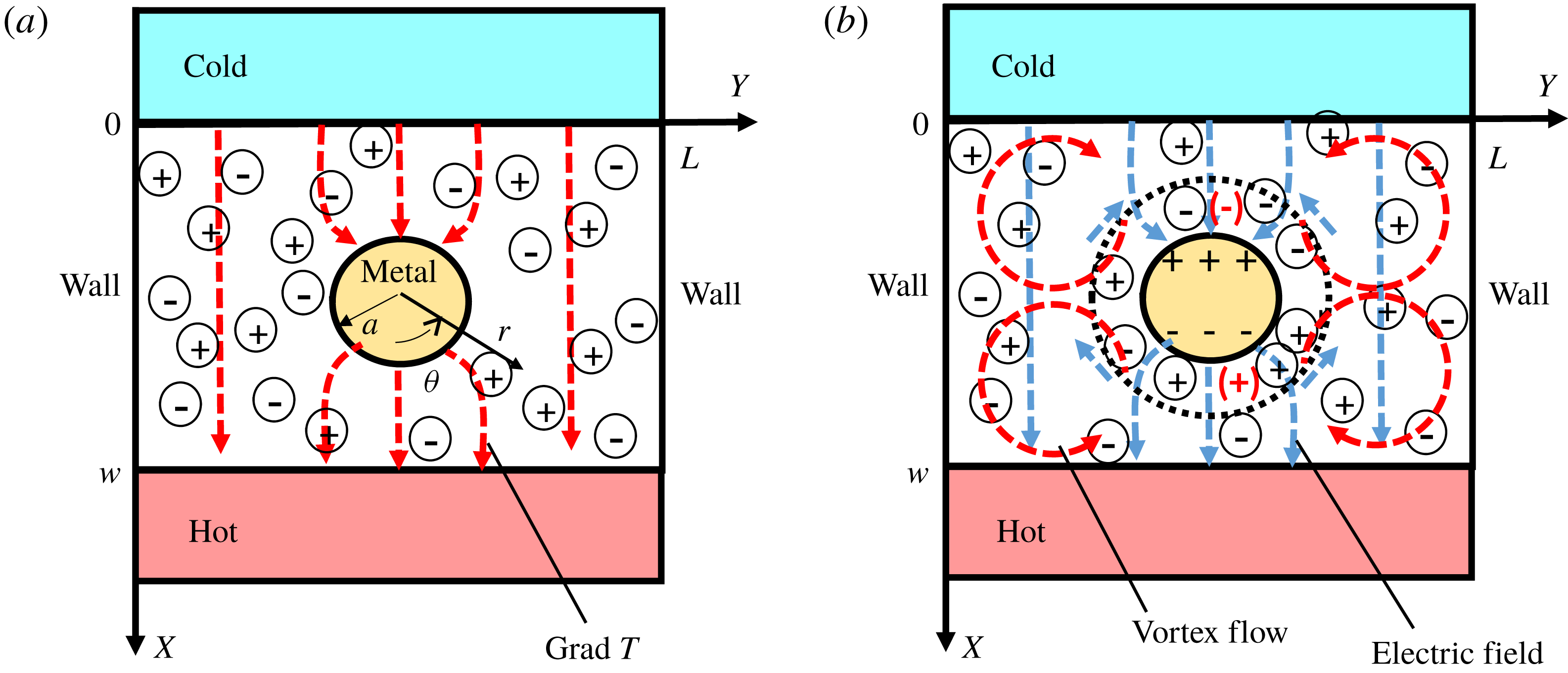
In figure 1, we consider a system having a metal cylinder of radius
 $a=0.1$
W at the centre position
 $(x,y)=(X/W,Y/W)=(0.5,0.75)$
in an electrolyte (typically water) between hot and cold parallel plates, for which the distance and length are
 $W~(=50~\unicode[STIX]{x03BC}\text{m})$
and
 $L~(=1.5~\text{W})$
, respectively. Since the thermal conductivity of a metal
 $\unicode[STIX]{x1D706}_{m}$
is usually much larger than that of the surrounding electrolyte
 $\unicode[STIX]{x1D706}_{e}$
, we can assume that
 $\unicode[STIX]{x1D706}_{m}=\infty$
. Furthermore, since the thermal diffusivity (of water) is also much larger than the molecular diffusivity, the temperature distribution becomes a steady state much faster than the ion distribution. Thus, the temperature around the metal cylinder can be approximated analytically (Sugioka Reference Sugioka2014b
) as
 $$\begin{eqnarray}T\simeq T_{a}+\left(1-\frac{a^{2}}{r^{2}}\right)(\unicode[STIX]{x1D735}T)_{0}r\cos \unicode[STIX]{x1D703},\end{eqnarray}$$
on the basis of the solution of the steady heat diffusion equation
 $\unicode[STIX]{x1D6FB}^{2}T=0$
for an unbounded problem, where
 $T_{a}(=300\,\text{K})$
is the temperature of the cylinder,
 $r$
is the radial coordinate and
 $\unicode[STIX]{x1D703}$
is the angular coordinate. Note that the effectiveness of (2.1) is also examined through our simulations.
Primitive mechanism and considered system of the nonlinear thermokinetic phenomenon (NTKP) in our direct simulation. Here,
 $(\unicode[STIX]{x1D735}T)_{a}(=~1\,\text{K}~\unicode[STIX]{x03BC}\text{m}^{-1})$
is an externally applied temperature gradient,
 $a=0.1~\text{W}$
is the radius of a metal cylinder and
 $W(=50~\unicode[STIX]{x03BC}\text{m})$
is the distance between the hot and cold boundaries.

2.2 Primitive mechanism
At temperature of (2.1), the positive and negative ions (e.g.
 $\text{H}^{+}$
and
 $\text{Cl}^{-}$
) move in the direction of the colder region along the heat flux, as shown in figure 1(a). However, because of the difference of the thermal diffusivity of the ions, net negative (positive) charge is generated in the colder (hotter) region of the metal cylinder. Thus, the counter-charges are induced on the surface of the metal cylinder and form an electric double layer. Note that, although the induced charge cancels the electric field in the diffused ion region, the tangential electric field remains. Thus, quadrupolar vortex flows are generated around the metal cylinder as shown in figure 1(b). Here, we neglect the convection flow due to the difference of the density as a first step since it is usually suppressed in a thermophoretic measurement.
2.3 Governing equations
We consider the Poisson equation, the extended Nernst–Planck (NP) equation including the thermokinetic diffusion term with the advection flow term, the diffusion–advection equation for the temperature field and the Stokes equation as follows:
 $$\begin{eqnarray}\displaystyle & \displaystyle \unicode[STIX]{x1D700}\unicode[STIX]{x1D6FB}^{2}\unicode[STIX]{x1D6F7}+\unicode[STIX]{x1D70C}=0, & \displaystyle\end{eqnarray}$$
 $$\begin{eqnarray}\displaystyle & \displaystyle \frac{\unicode[STIX]{x2202}C_{\pm }}{\unicode[STIX]{x2202}t}=-\unicode[STIX]{x1D735}\boldsymbol{\cdot }\left[-D_{\pm }\left(\unicode[STIX]{x1D735}C_{\pm }\pm \frac{ze}{kT}C_{\pm }\unicode[STIX]{x1D735}\unicode[STIX]{x1D6F7}+\frac{Q_{\pm }}{kT}C_{\pm }\frac{\unicode[STIX]{x1D735}T}{T}\right)+C_{\pm }\boldsymbol{u}\right], & \displaystyle\end{eqnarray}$$
 $$\begin{eqnarray}\displaystyle & \displaystyle \frac{\unicode[STIX]{x2202}T}{\unicode[STIX]{x2202}t}=-\unicode[STIX]{x1D735}\boldsymbol{\cdot }(-a_{T}\unicode[STIX]{x1D735}T+T\boldsymbol{u}), & \displaystyle\end{eqnarray}$$
 $$\begin{eqnarray}\displaystyle & \displaystyle -\unicode[STIX]{x1D735}P+\unicode[STIX]{x1D707}\unicode[STIX]{x1D6FB}^{2}\boldsymbol{u}-\unicode[STIX]{x1D70C}\unicode[STIX]{x1D735}\unicode[STIX]{x1D6F7}=0,\quad \unicode[STIX]{x1D735}\boldsymbol{\cdot }\boldsymbol{u}=0, & \displaystyle\end{eqnarray}$$
where
 $\unicode[STIX]{x1D700}=80\unicode[STIX]{x1D700}_{0}$
is the dielectric permittivity of the solvent (typically water),
 $\unicode[STIX]{x1D700}_{0}$
is the vacuum permittivity,
 $t$
is time,
 $\boldsymbol{u}_{d}[=(u_{x},u_{y})]$
is the flow velocity,
 $\unicode[STIX]{x1D6F7}$
is the potential,
 $\unicode[STIX]{x1D707}({\sim}1~\text{mPa}~\text{s})$
is the viscosity,
 $k$
is the Boltzmann constant,
 $P$
is the pressure,
 $ze$
is the ion charge and
 $\unicode[STIX]{x1D70C}~[=ze(C_{+}-C_{-})]$
is the charge density.
Furthermore,
 $C_{\pm }$
,
 $D_{\pm }$
and
 $Q_{\pm }$
are the ion concentration, the ion diffusivity and the ionic heat of transport, respectively, of the positive and negative ions;
 $a_{T}(=\unicode[STIX]{x1D706}/\unicode[STIX]{x1D70C}_{m}c)=148\times 10^{-9}~\text{m}^{2}~\text{s}^{-1}$
for water is the thermal diffusivity,
 $\unicode[STIX]{x1D706}$
is the thermal conductivity,
 $c$
is the specific heat, and
 $\unicode[STIX]{x1D70C}_{m}$
is the density of electrolyte.
2.4 Dimensionless formulations
It is useful to consider dimensionless formulations corresponding to (2.2)–(2.5) as follows:
 $$\begin{eqnarray}\displaystyle & \displaystyle 2\unicode[STIX]{x1D716}^{2}\unicode[STIX]{x1D6FB}_{n}^{2}\unicode[STIX]{x1D719}+\unicode[STIX]{x1D70C}_{n}=0, & \displaystyle\end{eqnarray}$$
 $$\begin{eqnarray}\displaystyle & \displaystyle \frac{\unicode[STIX]{x2202}c_{\pm }}{\unicode[STIX]{x2202}\unicode[STIX]{x1D70F}}=-\unicode[STIX]{x1D735}_{n}\boldsymbol{\cdot }\boldsymbol{f}_{\pm }, & \displaystyle\end{eqnarray}$$
 $$\begin{eqnarray}\displaystyle & \displaystyle \boldsymbol{f}_{\pm }=-\tilde{D}_{\pm }\left(\unicode[STIX]{x1D735}_{n}c_{\pm }\pm c_{\pm }\frac{\unicode[STIX]{x1D735}_{n}\unicode[STIX]{x1D719}}{\tilde{T}}+2\frac{\unicode[STIX]{x1D6FC}_{\pm }}{\tilde{T}}c_{\pm }\frac{\unicode[STIX]{x1D735}_{n}\tilde{T}}{\tilde{T}}\right)+c_{\pm }\boldsymbol{u}_{n}, & \displaystyle\end{eqnarray}$$
 $$\begin{eqnarray}\displaystyle & \displaystyle \frac{\unicode[STIX]{x2202}\tilde{T}}{\unicode[STIX]{x2202}\unicode[STIX]{x1D70F}}=-\unicode[STIX]{x1D735}_{n}\boldsymbol{\cdot }\left(-\frac{a_{T}}{D_{0}}\unicode[STIX]{x1D735}_{n}\tilde{T}+\tilde{T}\boldsymbol{u}\right), & \displaystyle\end{eqnarray}$$
 $$\begin{eqnarray}\displaystyle & \displaystyle -\unicode[STIX]{x1D735}_{n}p+\tilde{\unicode[STIX]{x1D707}}\unicode[STIX]{x1D6FB}_{n}^{2}\boldsymbol{u}_{n}-F_{0}\unicode[STIX]{x1D70C}_{n}\unicode[STIX]{x1D735}_{n}\unicode[STIX]{x1D719}=0,\quad \unicode[STIX]{x1D735}_{n}\boldsymbol{\cdot }\boldsymbol{u}_{n}=0, & \displaystyle\end{eqnarray}$$
where
 $\boldsymbol{u}_{n}(=~\boldsymbol{u}/u_{c})$
,
 $\unicode[STIX]{x1D719}(=~\unicode[STIX]{x1D6F7}/\unicode[STIX]{x1D6F7}_{c})$
,
 $c_{\pm }(=~C_{\pm }/C_{0})$
,
 $\unicode[STIX]{x1D70C}_{n}(=~\unicode[STIX]{x1D70C}/\unicode[STIX]{x1D70C}_{c}=c_{+}-c_{-})$
,
 $\unicode[STIX]{x1D70F}(=~t/T_{0})$
,
 $p(=~P/P_{c})$
,
 $\tilde{T}(=~T/T_{a})$
,
 $\tilde{\unicode[STIX]{x1D707}}(=~\unicode[STIX]{x1D707}/\unicode[STIX]{x1D707}_{0})$
,
 $\tilde{D_{\pm }}(=~D_{\pm }/D_{0})$
and
 $(x,y)[=~(x/W,Y/W)]$
are the non-dimensional values of the flow velocity, potential, concentration, charge density, time, pressure, temperature, viscosity, diffusivity and position, respectively. Further,
 $\unicode[STIX]{x1D735}_{n}=\unicode[STIX]{x1D735}/W$
,
 $\unicode[STIX]{x1D716}=\unicode[STIX]{x1D706}_{D}/W$
,
 $\boldsymbol{f}_{+}$
(
 $\boldsymbol{f}_{-}$
) is a non-dimensional flux of a positive (negative) ion,
 $\unicode[STIX]{x1D706}_{D}(\equiv \sqrt{\unicode[STIX]{x1D700}kT_{a}/2z^{2}e^{2}C_{0}})$
denotes the Debye length,
 $T_{0}(=~W^{2}/D_{0})$
(typically, 2.5 s) is a diffusion time,
 $F_{0}=kT_{a}C_{0}T_{0}/\unicode[STIX]{x1D707}_{0}$
is a non-dimensional number related to the strength of the Coulomb force;
 $T_{a}$
(300 K),
 $\unicode[STIX]{x1D707}_{0}$
(1 mPa s),
 $D_{0}$
(
 $10^{-9}~\text{m}^{2}~\text{s}^{-1}$
),
 $u_{c}=W/T_{0}$
(typically, 20
 $\unicode[STIX]{x03BC}\text{m}~\text{s}^{-1}$
),
 $P_{c}=\unicode[STIX]{x1D707}_{0}/T_{0}$
,
 $\unicode[STIX]{x1D6F7}_{c}=kT_{a}/ze$
and
 $\unicode[STIX]{x1D70C}_{c}=zeC_{0}$
are the reference values of the temperature, viscosity, diffusivity, flow velocity, pressure, potential and charge density, respectively. Furthermore, we define
 $\unicode[STIX]{x1D6FC}_{\pm }$
as follows:
 $$\begin{eqnarray}\unicode[STIX]{x1D6FC}_{\pm }=\frac{Q_{\pm }}{2kT_{a}}.\end{eqnarray}$$
2.5 Considered modes (Modes 1–6)
2.5.1 Boundary conditions
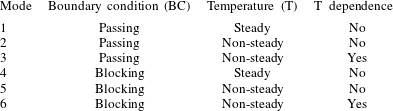
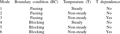
We summarize the considered modes in table 1. We assume a passing boundary condition at the edges for Modes 1–3, whereas we assume a blocking boundary condition for Modes 4–6; i.e. at
 $x=0$
and 1,
 $$\begin{eqnarray}\displaystyle & \displaystyle \boldsymbol{f}_{\pm }\neq 0\quad (\text{for passing problems}), & \displaystyle\end{eqnarray}$$
 $$\begin{eqnarray}\displaystyle & \displaystyle \boldsymbol{f}_{\pm }=0\quad (\text{for blocking problems}). & \displaystyle\end{eqnarray}$$
Here, the ion passing condition means that ions at the colder edge (i.e.
 $x=0$
) can diffuse to the hotter edge (i.e.
 $x=1$
) promptly through an external electrical circuit; i.e. we use a kind of periodic boundary condition for ion transportation and we assume an artificial flux (Sugioka Reference Sugioka2014a
) to expel the ion near the edges as
 $$\begin{eqnarray}\displaystyle \boldsymbol{f}_{\pm }=-\bar{\tilde{D_{\pm }}}\frac{c_{\pm }^{x=\unicode[STIX]{x0394}x/2}-c_{\pm }^{1-\unicode[STIX]{x0394}x/2}}{x_{m}}\boldsymbol{i}, & & \displaystyle\end{eqnarray}$$
where
 $\boldsymbol{i}$
is a unit vector in the direction of
 $x$
,
 $\unicode[STIX]{x0394}x_{m}$
is the
 $x$
width of the upper and lower cells next to the upper and lower edges in the finite volume method (FVM) for the NP equation, and
 $\bar{\tilde{D_{\pm }}}~[=(D_{\pm }^{x=0}+D_{\pm }^{x=1})/2]$
is the average ion diffusivity at the edges. Physically, the ion passing condition has various meanings as discussed in appendix C of Sugioka (Reference Sugioka2014a
); e.g. it corresponds to an experiment using an idealized thermogalvanic cell, in which the chemical reactions are assumed to occur at the edges. However, here we use it just as the better approximation for the unbounded problem, since the chemical reactions due to thermophoresis are very complex phenomena and beyond the scope of this paper.
List of modes.
Further, the ion blocking condition means that ions next to the assumed wall at the edges cannot pass them and physically this corresponds to a thermophoretic experiment using a glass chamber or open electrodes that do not go through a Faraday current. Note that we do not consider the zero-electric-field boundary condition that is often used at the wall in a glass chamber (Chikina et al.
Reference Chikina, Shikin and Varlamov2012, Reference Chikina, Shikin and Varlamov2015; Majee & Würger Reference Majee and Würger2012), since it is more artificial than our method in which ions cannot go through the wall at the edges. In addition, we also assume the ion blocking condition on the metal cylinder for all of the modes; i.e.
 $\boldsymbol{f}_{\pm }=0$
at
 $\tilde{r}=0.1$
. Further, we assume that the flow velocity is zero at the left and right walls, the upper and lower plates and the surface of the metal cylinder; i.e.
 $\boldsymbol{u}_{n}=0$
at
 $x=0$
and 1,
 $y=0$
and 1.5 and
 $\tilde{r}=0.1$
. Furthermore, for simplicity, we assume that
 $\unicode[STIX]{x1D6F7}=0$
on the surface of the metal cylinder.
2.5.2 Calculation method of the temperature
We assume (2.1) for Modes 1 and 4, whereas we consider the non-steady temperature obtained by (2.9) under the condition that
 $\tilde{T}(x,y)=1$
at
 $\unicode[STIX]{x1D70F}=0$
for Modes 2, 3, 5 and 6. In (2.9),
 $a_{T}/D_{0}$
(typically, 148 for water) is the non-dimensional number related to the thermal and ion diffusivities; since
 $a_{T}/D_{0}\gg 1$
, we can assume (2.1) if we are not interested in the non-steady effect. Note that the non-dimensional form of (2.1) is
 $$\begin{eqnarray}\tilde{T}\simeq 1+\left(1-\frac{\tilde{a}^{2}}{\tilde{r}^{2}}\right)(\unicode[STIX]{x1D735}_{n}\tilde{T})_{0}\tilde{r}\cos \unicode[STIX]{x1D703},\end{eqnarray}$$
where
 $\tilde{a}=(a/W)$
,
 $\tilde{r}=(r/W)$
and
 $(\unicode[STIX]{x1D735}_{n}\tilde{T})_{0}=(\unicode[STIX]{x1D735}_{n}T)_{0}(W/T_{a})$
(typically,
 $(1~\text{K}/1~\unicode[STIX]{x03BC}\text{m})\times (50~\unicode[STIX]{x03BC}\text{m}/300~\text{K})=0.167$
). Since the initial temperature distribution (
 $\tilde{T}(x,y)=1$
or (2.15)) may affect the result of a flow velocity in steady state, we examine the effect in this paper.
2.5.3 Temperature dependence of the parameters
The temperature around the metal cylinder is
 $T_{a}$
and our concerned phenomena can be generated in an electric double layer of thickness
 $\unicode[STIX]{x1D706}_{D}$
(1
 $\unicode[STIX]{x03BC}\text{m}$
, throughout this paper); i.e. the temperature difference of the concerned region is approximately 2 K. Thus, the effects of the temperature dependence are assumed to be small. Nevertheless, one may criticize that the variation of the coefficients of viscosity
 $\unicode[STIX]{x1D707}$
, electrophoretic and thermophoretic mobility and ion diffusivity cannot be negligible. Thus, we examine these effects in this paper. However, it is not a good idea to consider the complex temperature dependence of all parameters from the beginning since we cannot recognize the main effects of our system because of the complexity. Thus, we assume the temperature dependence only for Modes 3 and 6.
Specifically, for a dilute HCl solution, we assume as follows:
 $$\begin{eqnarray}\displaystyle & \displaystyle \tilde{\unicode[STIX]{x1D707}}=\tilde{a}_{\unicode[STIX]{x1D707}}\exp \left(\frac{\tilde{b}_{\unicode[STIX]{x1D707}}}{\tilde{T}}\right), & \displaystyle\end{eqnarray}$$
 $$\begin{eqnarray}\displaystyle & \displaystyle \tilde{D_{\pm }}=\tilde{a}_{\pm }\exp \left(\frac{-\tilde{b}_{\pm }}{\tilde{T}}\right), & \displaystyle\end{eqnarray}$$
where (2.16) is known as the Andrade equation (Andrade Reference Andrade1952) and the parameters are determined from the well-known data for water (JSME 2009) as
 $\tilde{a}_{\unicode[STIX]{x1D707}}=1.369$
and
 $\tilde{b}_{\unicode[STIX]{x1D707}}=6.475$
; equation (2.17) is known as the Arrhenius equation and the parameters are determined by the data in Li & Gregory (Reference Li and Gregory1974) as
 $\tilde{a}_{+}=2358$
and
 $\tilde{b}_{+}=5.500$
for a
 $\text{H}^{+}$
ion, and
 $\tilde{a}_{-}=4169$
and
 $\tilde{b}_{-}=7.580$
for a
 $\text{Cl}^{-}$
ion. Further, electroosmotic mobilities for positive and negative ions are described by the Einstein relation as
 $$\begin{eqnarray}\unicode[STIX]{x1D705}_{e,\pm }=\frac{D_{\pm }}{kT},\end{eqnarray}$$
and it is already considered in (2.3). Thus, by using (2.17), the temperature dependence of
 $\unicode[STIX]{x1D705}_{e,\pm }$
is considered completely. Furthermore, thermoosmotic mobilities for positive and negative ions are described as
 $$\begin{eqnarray}\unicode[STIX]{x1D705}_{T,\pm }=\unicode[STIX]{x1D705}_{e,\pm }S_{\pm }=\frac{D_{\pm }}{kT}\frac{Q_{\pm }}{T},\end{eqnarray}$$
as already considered in (2.3). Here,
 $S_{\pm }=(Q_{\pm }/T)$
is the Eastman entropy for positive and negative ions. Thus, by considering (2.16) and (2.17), the temperature dependence of
 $\unicode[STIX]{x1D705}_{T,\pm }$
is considered almost completely. Note that Eastman’s heat of transfer is often measured under the condition of a temperature difference of 20 K (Agar Reference Agar, Delahay and Tobias1963) and thus the temperature dependence of
 $Q_{\pm }$
is usually considered to be neglected.
2.6 Numerical method using a multi-physics simulation technique
We use the finite volume method (FVM) for the NP part and the heat conduction part to ensure the ion conserving condition, whereas we use the finite element method (FEM) for the parts of the Poisson and Stokes equations to ensure the accuracy of the calculations; i.e. our calculations are performed in the framework of the FVM–FEM coupling method described in Sugioka (Reference Sugioka2014a
). Specifically, we first generate unstructured meshes around the metal cylinder and structured meshes at positions far from the cylinder; then, for the completely non-steady calculations (Modes 2, 3, 5 and 6 in table 1), we solve the heat conduction equation of (2.9) by the FVM, the extended NP equation of (2.7) by the FVM, the Poisson equation of (2.6) by the FEM and the Stokes equation of (2.10) by the FEM, iteratively. Further, for the incompletely non-steady calculations (Modes 1 and 4 in table 1), we use the solution of (2.15) without solving (2.9). Note that most of the algorithms of our calculations are the same as those described in appendix A of Sugioka (Reference Sugioka2014a
) except in terms of the thermophoretic motions of the ions. Thus, here, we briefly describe the main differences; since the difference of
 $\tilde{D}_{+}$
and
 $\tilde{D}_{-}$
is intrinsic for non-equilibrium thermokinetic study, we consider the discretized matrix formulation of the PN part (equations (2.7) and (2.8)) for the FVM as follows:
 $$\begin{eqnarray}\displaystyle & & \displaystyle \left(1+\mathop{\sum }_{j}^{j=4}\tilde{D}_{\pm ,ij}G_{ij}^{A}\right)c_{\pm }^{i,n+1}-\mathop{\sum }_{j}^{j=4}\tilde{D}_{\pm ,ij}G_{ij}^{A}c_{\pm }^{j,n}=c_{\pm }^{i,n}\mp \mathop{\sum }_{j}^{j=4}\frac{\tilde{D}_{\pm ,ij}}{\tilde{T}^{ij,n}}G_{ij}^{A}c_{\pm ,ij}^{n+1}\unicode[STIX]{x1D6FF}\unicode[STIX]{x1D719}^{ij,n}\nonumber\\ \displaystyle & & \displaystyle \qquad \quad -\,\mathop{\sum }_{j}^{j=4}G_{ij}^{B}c_{\pm ,ij}^{n}\boldsymbol{u}_{ij}^{n}\boldsymbol{\cdot }\boldsymbol{n}_{ij}-\mathop{\sum }_{j}^{j=4}\frac{2\tilde{D}_{\pm ,ij}\unicode[STIX]{x1D6FC}_{\pm }}{(\tilde{T}^{ij,n})^{2}}G_{ij}^{A}c_{\pm ,ij}^{n}\unicode[STIX]{x1D6FF}\tilde{T}^{ij,n},\end{eqnarray}$$
where
 $\unicode[STIX]{x1D6FF}\unicode[STIX]{x1D719}^{ij,n}=\unicode[STIX]{x1D719}^{i,n}-\unicode[STIX]{x1D719}^{j,n}$
,
 $\unicode[STIX]{x1D6FF}\tilde{T}^{ij,n}=\tilde{T}^{i,n}-\tilde{T}^{j,n}$
,
 $\tilde{T}^{ij,n}=(\tilde{T}^{i,n}+\tilde{T}^{j,n}/2)$
,
 $G_{ij}^{A}=(\unicode[STIX]{x0394}tS_{ij}/V_{i}d_{ij})(\,\boldsymbol{j}_{ij}\boldsymbol{\cdot }\boldsymbol{n}_{ij})$
, and
 $G_{ij}^{B}=(\unicode[STIX]{x0394}tS_{ij}/V_{i})$
. Here,
 $V_{i}$
is the volume of the
 $i$
th finite element at
 $\boldsymbol{x}_{i}$
,
 $S_{ij}$
is the boundary area and
 $\boldsymbol{n}_{ij}$
is the outward unit vector normal to
 $S_{ij}$
. Further,
 $\boldsymbol{u}_{ij}^{n}$
is the velocity between the
 $i$
th and
 $j$
th cells,
 $c_{\pm ,ij}^{n}=(c_{\pm }^{i,n}+c_{\pm }^{j,n})/2$
,
 $d_{ij}$
is the distance between the
 $i$
th and
 $j$
th centre points,
 $\unicode[STIX]{x1D719}^{i,n+1}(=(1/4)\sum _{\unicode[STIX]{x1D6FD}=1}^{4}\unicode[STIX]{x1D719}_{\unicode[STIX]{x1D6FD}})$
is the centre value of
 $\unicode[STIX]{x1D719}$
at the
 $i$
th cell,
 $\boldsymbol{j}_{ij}=(\boldsymbol{x}^{j}-\boldsymbol{x}^{i})/|\boldsymbol{x}^{j}-\boldsymbol{x}^{i}|$
, and the suffixes
 $n$
and
 $n+1$
show the value at
 $t=t_{n}$
and
 $t_{n+1}$
, respectively.
2.7 Simple analytical theory
We consider a simple analytical theory based on Sugioka (Reference Sugioka2014b ) as follows:
 $$\begin{eqnarray}\displaystyle & \displaystyle u^{max}=fu_{ntkp}, & \displaystyle\end{eqnarray}$$
 $$\begin{eqnarray}\displaystyle & \displaystyle u_{ntkp}=\frac{\unicode[STIX]{x1D700}a}{\unicode[STIX]{x1D707}}E_{ntkp}^{2}, & \displaystyle\end{eqnarray}$$
 $$\begin{eqnarray}\displaystyle & \displaystyle E_{ntkp}=S_{e}(\unicode[STIX]{x1D735}T)_{0}, & \displaystyle\end{eqnarray}$$
 $$\begin{eqnarray}\displaystyle & \displaystyle S_{e}=\frac{D_{+}\unicode[STIX]{x1D6FC}_{+}-D_{-}\unicode[STIX]{x1D6FC}_{-}}{D_{+}+D_{-}}\frac{2k}{eZ}, & \displaystyle\end{eqnarray}$$
where
 $S_{e}$
is a Seebeck coefficient (e.g.
 $S_{e}=374~\unicode[STIX]{x03BC}\text{V}~\text{K}^{-1}$
for a HCl solution);
 $u_{ntkp}$
and
 $E_{ntkp}$
are the theoretical maximum flow velocity and electric field predicted for the unbounded problem (Sugioka Reference Sugioka2014b
) of the nonlinear thermokinetic phenomena; e.g.
 $u_{ntkp}=0.495~\unicode[STIX]{x03BC}\text{m}~\text{s}^{-1}$
and
 $E_{ntkp}=374~\text{V}~\text{m}^{-1}$
at
 $(\unicode[STIX]{x1D735}T)_{0}=1~\text{K}~\unicode[STIX]{x03BC}\text{m}^{-1}$
;
 $f$
is the relative magnification factor for the maximum flow velocity and it is determined by the numerical value of
 $u^{max}$
at
 $(\unicode[STIX]{x1D735}T)_{0}=1~\text{K}~\unicode[STIX]{x03BC}\text{m}^{-1}$
. Note that although an analytical expression for the NTKP velocity is described as
 $u_{ntkp}^{slip}=2u_{ntkp}$
(Sugioka Reference Sugioka2014b
),
 $u_{ntkp}$
provides the maximum peak value observed in numerical calculations because of the boundary condition that
 $\boldsymbol{u}=0$
.
3 Results
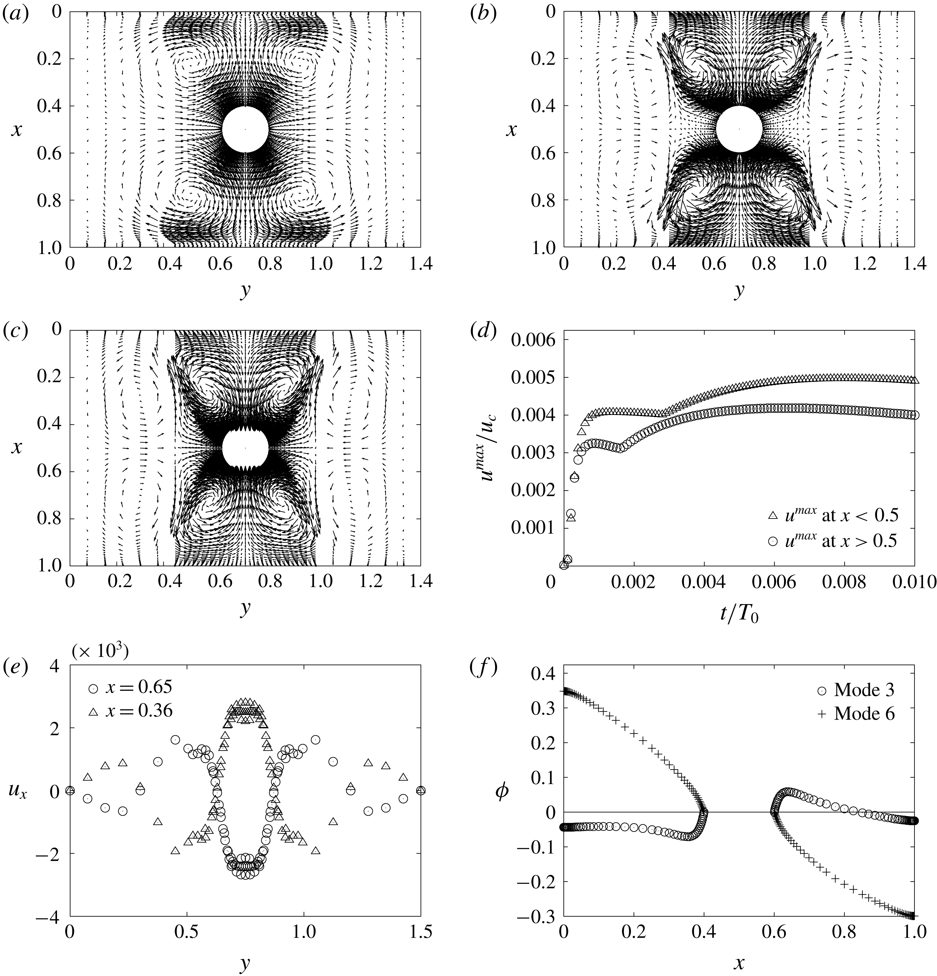
3.1 NTKP vortex flows in Mode 1
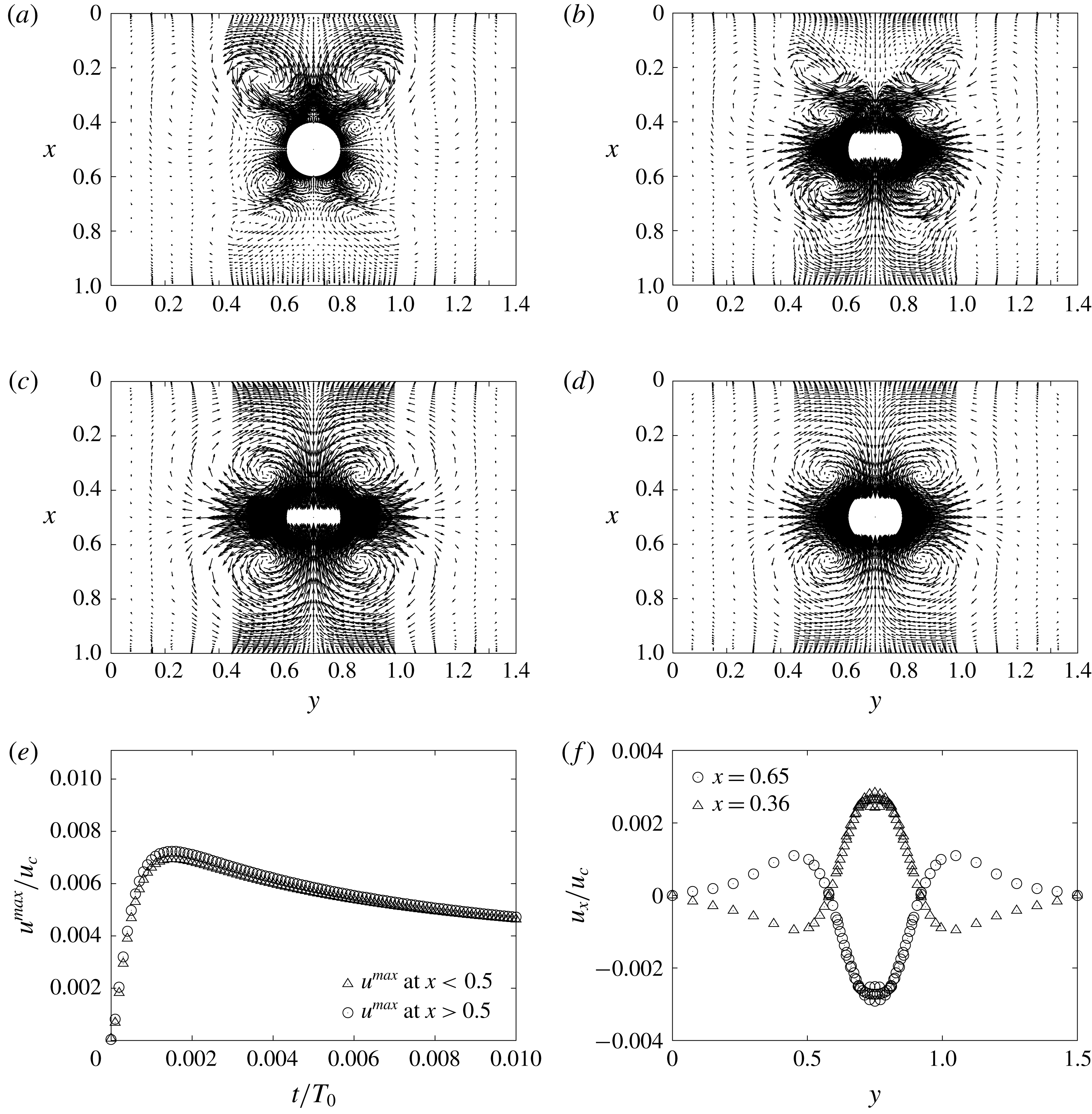
NTKP vortex flows in Mode 1. (a) AVF at
 $t/T_{0}=2\times 10^{-5}$
(
 $f^{\prime }=200$
). (b) AVF and SVF at
 $t/T_{0}=1\times 10^{-4}$
(
 $f^{\prime }=30$
). (c) SVF at
 $t/T_{0}=1.5\times 10^{-3}$
(
 $f^{\prime }=3$
). (d) SVF at
 $t/T_{0}=1\times 10^{-2}$
(
 $f^{\prime }=3$
). (d) Dependence of
 $u^{max}$
on
 $t$
. (e) Dependence of
 $u_{x}$
on
 $y$
at
 $t/T_{0}=1\times 10^{-2}$
.
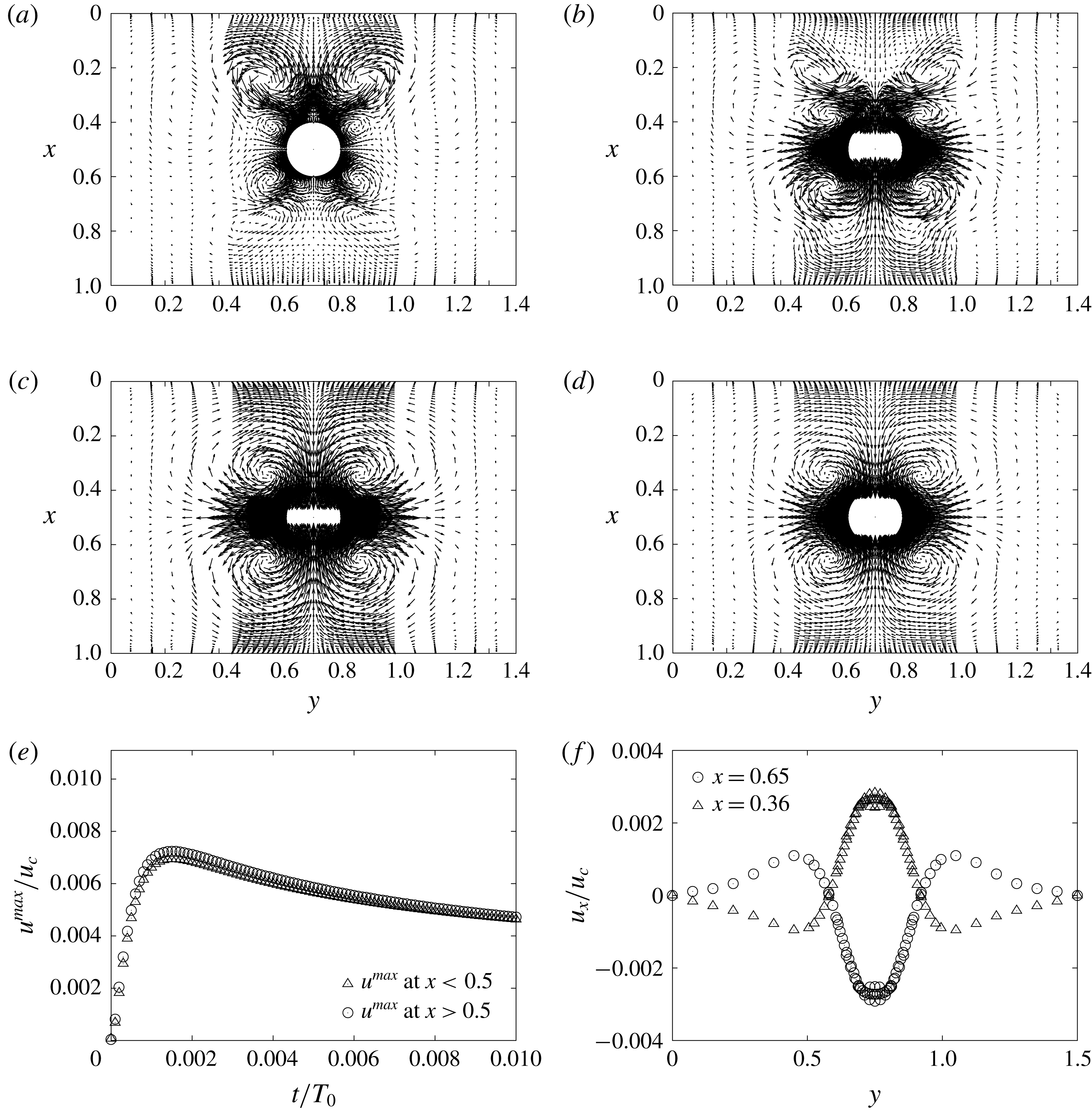
Figure 2 shows the NTKP vortex flows in Mode 1. Here,
 $(\unicode[STIX]{x1D735}T)_{0}=1~\text{K}~\unicode[STIX]{x03BC}\text{m}^{-1}$
,
 $f^{\prime }$
is the relative magnification factor for the flow vector,
 $T_{0}=W^{2}/D_{0}(=~2.5~\text{s})$
is a diffusion time,
 $a/W=0.1$
,
 $W=50~\unicode[STIX]{x03BC}\text{m}$
,
 $D_{0}=10^{-9}~\text{m}^{2}~\text{s}^{-1}$
,
 $u_{c}=W/T_{0}(=~20~\unicode[STIX]{x03BC}\text{m}~\text{s}^{-1})$
is the reference flow velocity,
 $D_{-}=2.03D_{0}$
,
 $\unicode[STIX]{x1D6FC}_{+}=2.666$
,
 $\unicode[STIX]{x1D6FC}_{-}=0.106$
,
 $D_{+}=9.31D_{0}$
,
 $Q_{-}=0.53~\text{kJ}~\text{mol}^{-1}$
,
 $Q_{+}=13.3~\text{kJ}~\text{mol}^{-1}$
,
 $C_{0}=10^{-7}~\text{mol}~\text{l}^{-1}$
,
 $\unicode[STIX]{x1D706}_{D}=1~\unicode[STIX]{x03BC}\text{m}$
and
 $F_{0}=623.6$
. Note that the same parameters are used throughout this paper except
 $(\unicode[STIX]{x1D735}T)_{0}$
. At
 $t/T_{0}=2\times 10^{-5}$
(in figure 2
a), we initially observe an anomalous vortex flow (AVF) around a metal cylinder; then, at
 $t/T_{0}=1\times 10^{-4}$
(in figure 2
b), we observe a standard vortex flow (SVF) at
 $x>0.3$
and the AVF at
 $x<0.3$
, where the flow direction of the AVF is opposite to that of the SVF (at steady state). Gradually, the AVF fades out until
 $t/T_{0}\simeq 2\times 10^{-4}$
; the SVF grows until
 $t/T_{0}\simeq 1.5\times 10^{-3}$
(in figure 2
c); then, the SVF gradually decays and reaches a quasi-steady state at
 $t/T_{0}\simeq 1\times 10^{-2}$
(in figure 2
d). Thus, our previous prediction (Sugioka Reference Sugioka2014b
) for the NTKP is correct as a whole. Moreover, figure 2(e) shows the dependence of
 $u^{max}$
on
 $t$
, where
 $u^{max}$
is the maximum value of
 $|\boldsymbol{u}|$
. In figure 2(e),
 $u^{max}$
has the peak value (
 $u^{max,peak}\simeq 0.007u_{c}=0.14~\unicode[STIX]{x03BC}\text{m}~\text{s}^{-1}$
) at
 $t/T_{0}=1.5\times 10^{-3}$
. Further, the flow velocity of the SVF in a steady state is almost symmetrical to the plane
 $x=0.5$
, as shown in figure 2(f).
3.2 NTKP vortex flows in Mode 3
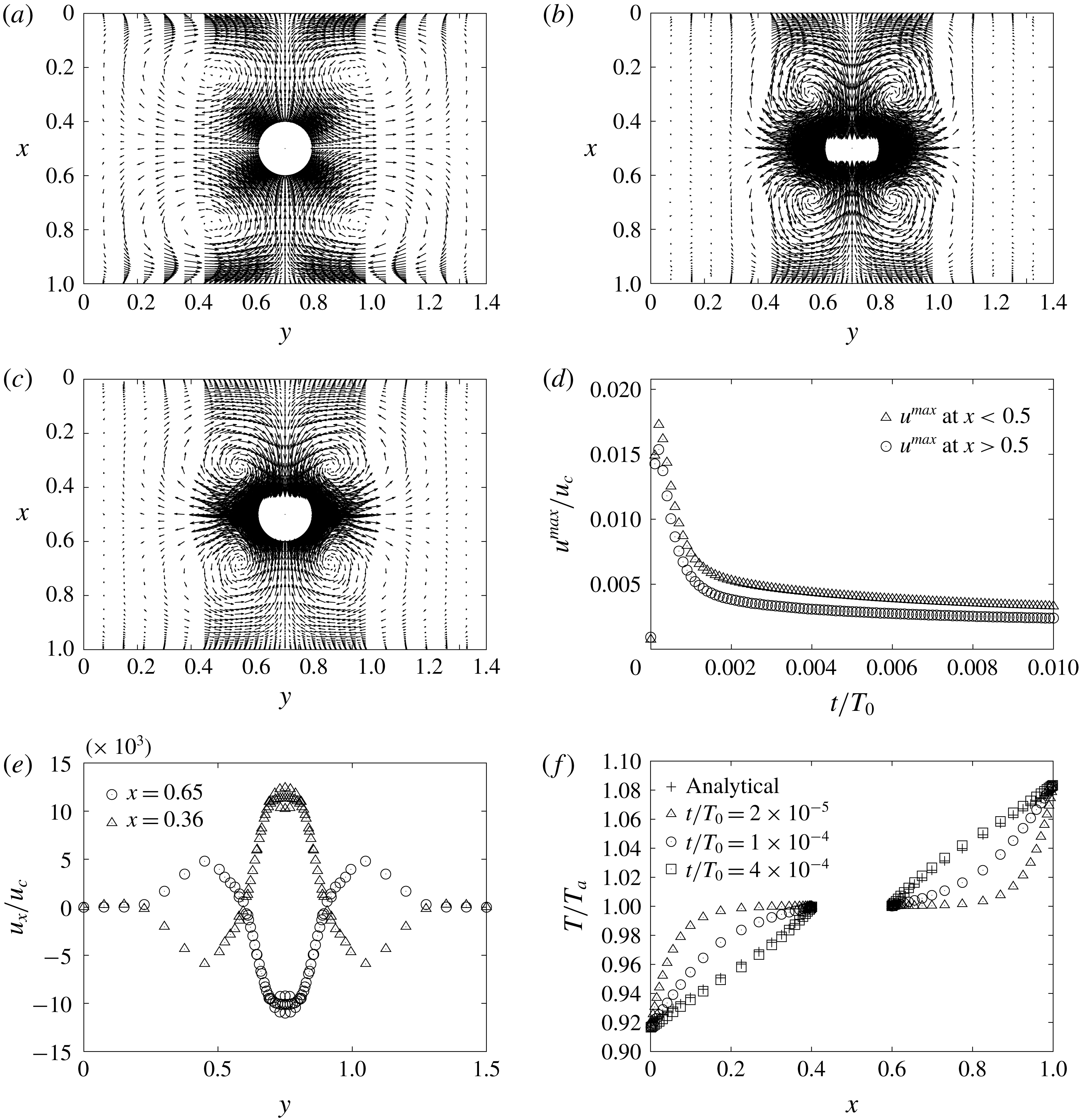
NTKP vortex flow in Mode 3. (a) SVF at
 $t/T_{0}=2\times 10^{-5}$
(
 $f^{\prime }=8$
). (b) SVF at
 $t/T_{0}=2\times 10^{-4}$
(
 $f^{\prime }=1$
). (c) SVF at
 $t/T_{0}=2\times 10^{-3}t$
(
 $f^{\prime }=3$
). (d) Dependence of
 $u^{max}$
on
 $t$
. (e) Dependence of
 $u_{x}$
on
 $y$
at
 $t/T_{0}=2\times 10^{-4}$
. (f) Dependence of
 $\tilde{T}$
on
 $x$
at
 $y=0.75$
.
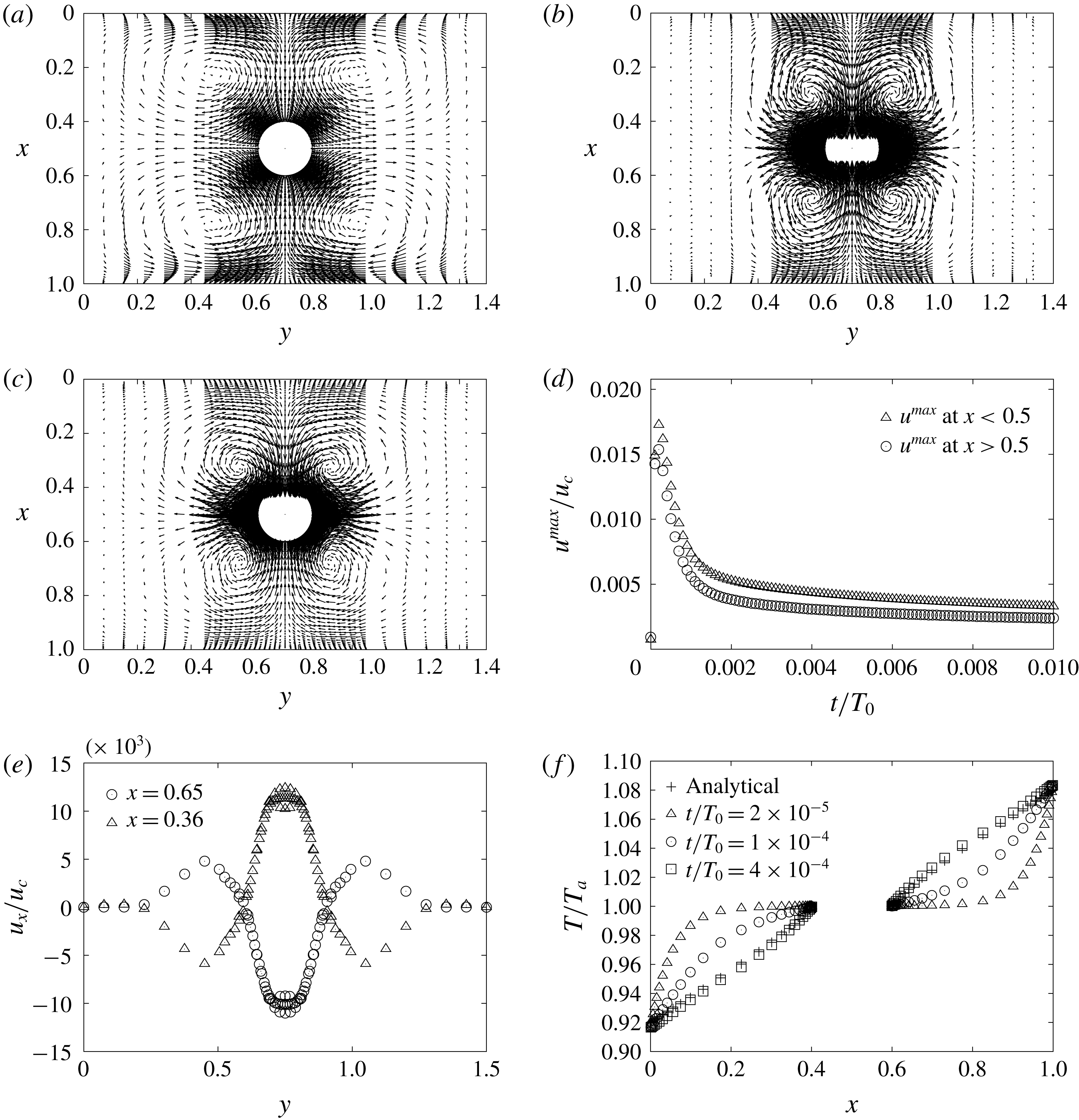
Figure 3 shows the NTKP vortex flows in Mode 3. At
 $t/T_{0}=2\times 10^{-5}$
(in figure 3
a), different from the result of Mode 1, we initially observe a moderately strong SVF around a metal cylinder; then, the velocity of the SVF grows rapidly until
 $t/T_{0}<2\times 10^{-4}$
(in figure 3
b); then, it decays with a time constant
 $\unicode[STIX]{x1D70F}^{decay,mode3}\simeq 0.002$
and reaches a quasi-steady state at
 $t/T_{0}=0.002$
(in figure 3
c). Further, figure 3(d) shows the dependence of
 $u^{max}$
on
 $t$
. In figure 3(d),
 $u^{max}$
has the peak value (
 $u^{max,peak}\simeq 0.019u_{c}=0.38~\unicode[STIX]{x03BC}\text{m}~\text{s}^{-1}$
) at
 $t/T_{0}=2.0\times 10^{-4}$
. Further, from figure 3(e), we find that the velocity of the SVF in a peak state is approximately symmetrical to the plane
 $x=0.5$
similar to Mode 1. In addition, since
 $u^{max}$
of Mode 3 at
 $x>0.002$
is almost the same as that of Mode 1, Modes 1 and 3 show similar characteristics as a whole except the transient period of the temperature at
 $t/T_{0}<10^{-4}$
. Figure 3(f) shows the dependence of temperature on
 $x$
at
 $y=0.75$
at
 $t/T_{0}=2.0\times 10^{-5}$
,
 $1.0\times 10^{-4}$
and
 $4.0\times 10^{-4}$
. In figure 3(f), the numerical results of the temperature distribution at
 $t/T_{0}\geqslant 0.4\times 10^{-3}$
are in good agreement with the analytical results. However, the temperature gradient at
 $t/T_{0}=2.0\times 10^{-5}$
is very steep; thus, leading to a large thermophoretic velocity at the edges.
3.3 NTKP vortex flows in Mode 6
NTKP vortex flow in Mode 6. (a) SVF at
 $t/T_{0}=2\times 10^{-5}$
(
 $f^{\prime }=400$
). (b) 8-pole vortex flow at
 $t/T_{0}=2\times 10^{-4}$
(
 $f^{\prime }=15$
). (c) 8-pole vortex flow at
 $t/T_{0}=2\times 10^{-3}$
(
 $f^{\prime }=3$
). (d) Dependence of
 $u^{max}$
on
 $t$
. (e) Dependence of
 $u_{x}$
on
 $y$
at
 $t/T_{0}=0.002$
. (f) Dependence of
 $\unicode[STIX]{x1D719}$
on
 $x$
at
 $y=0.75$
at
 $t/T_{0}=0.002$
.
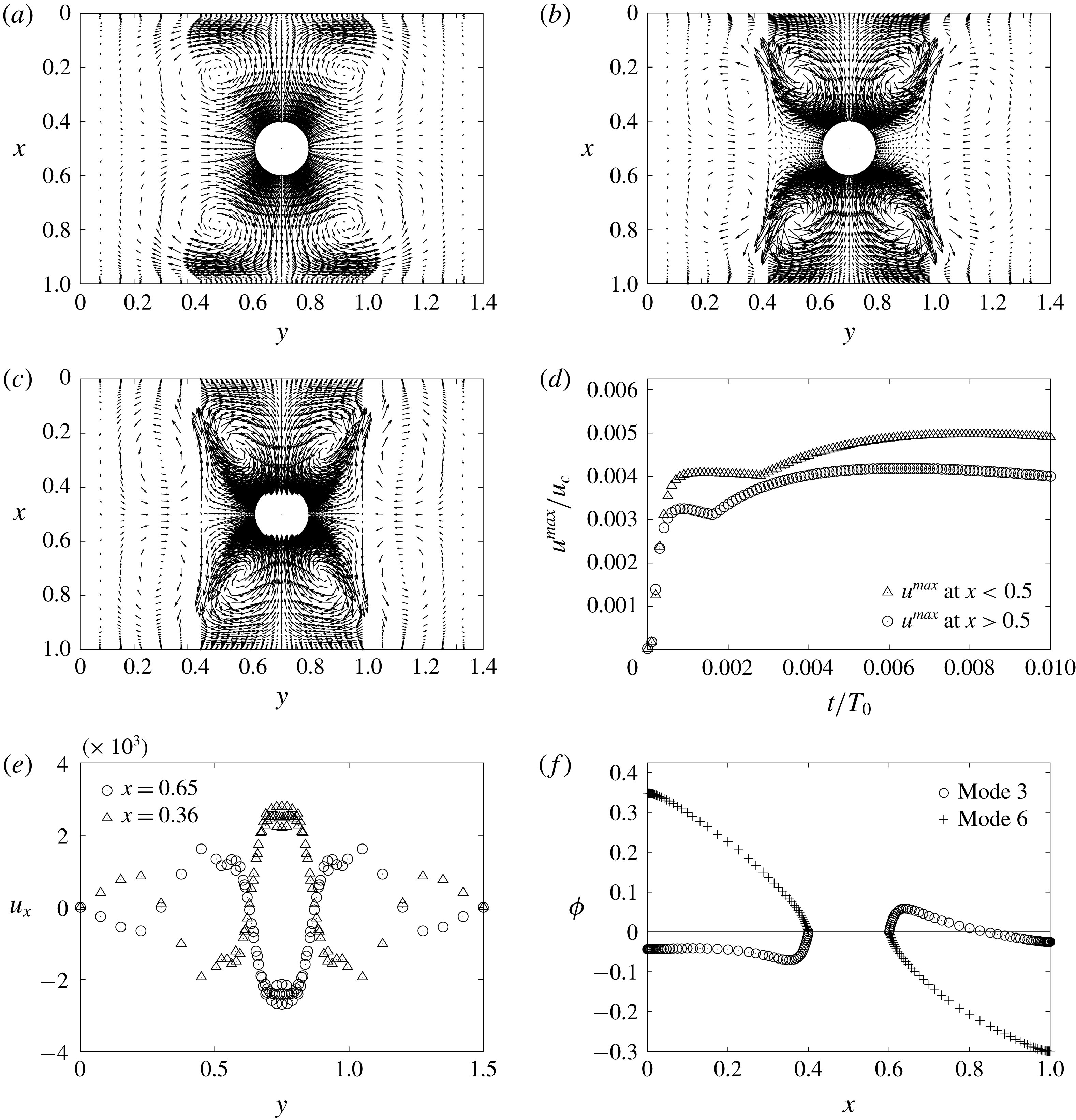
Figure 4 shows the NTKP vortex flows in Mode 4. Surprisingly, different from the result in Mode 3, we observe only a very weak SVF at
 $t/T_{0}=2\times 10^{-5}$
in figure 4(a); then, we observe an 8-pole vortex flow at
 $t/T_{0}=2\times 10^{-4}$
and
 $2\times 10^{-3}$
in figure 4(b,c). Figure 4(d) shows the dependence of
 $u^{max}$
on
 $t$
. In figure 4(d), the response time of Mode 6 is
 ${\sim}0.001T_{0}$
(i.e.
 $\unicode[STIX]{x1D70F}_{Mode6}\simeq 0.001T_{0}$
) and
 $u_{max}$
at
 $x<0.5$
is slightly larger than that at
 $x>0.5$
, although
 $u_{x}$
is almost symmetrical to the plain
 $x=0.5$
in figure 4(e). Further, in figure 4(e), we observe the complex change of the flow direction corresponding to the 8-pole vortex flow. Figure 4(f) shows the dependence of
 $\unicode[STIX]{x1D719}$
on
 $x$
for Modes 3 and 6. From figure 4(f), we can recognize that the blocking boundary condition forms much larger potential difference than the passing boundary condition. Here, owing to the blocking boundary condition, the electric field in the
 $x$
direction due to the Seebeck effect not only suppresses the nonlinear thermokinetic phenomena but also induces a different type of NTKP vortex, which will be discussed later.
3.4 NTKP characteristics
Nonlinear dependence of
 $u_{max}$
on
 $(\unicode[STIX]{x1D735}T)_{0}$
. (a) NTKP (passing BC,
 $t/T_{0}=0.02$
). (b) NTKP (blocking BC,
 $t/T_{0}=0.02$
). (c) NTKP of Mode 2 at the peak time. (d) NTKP of Mode 3 at the peak and steady states.

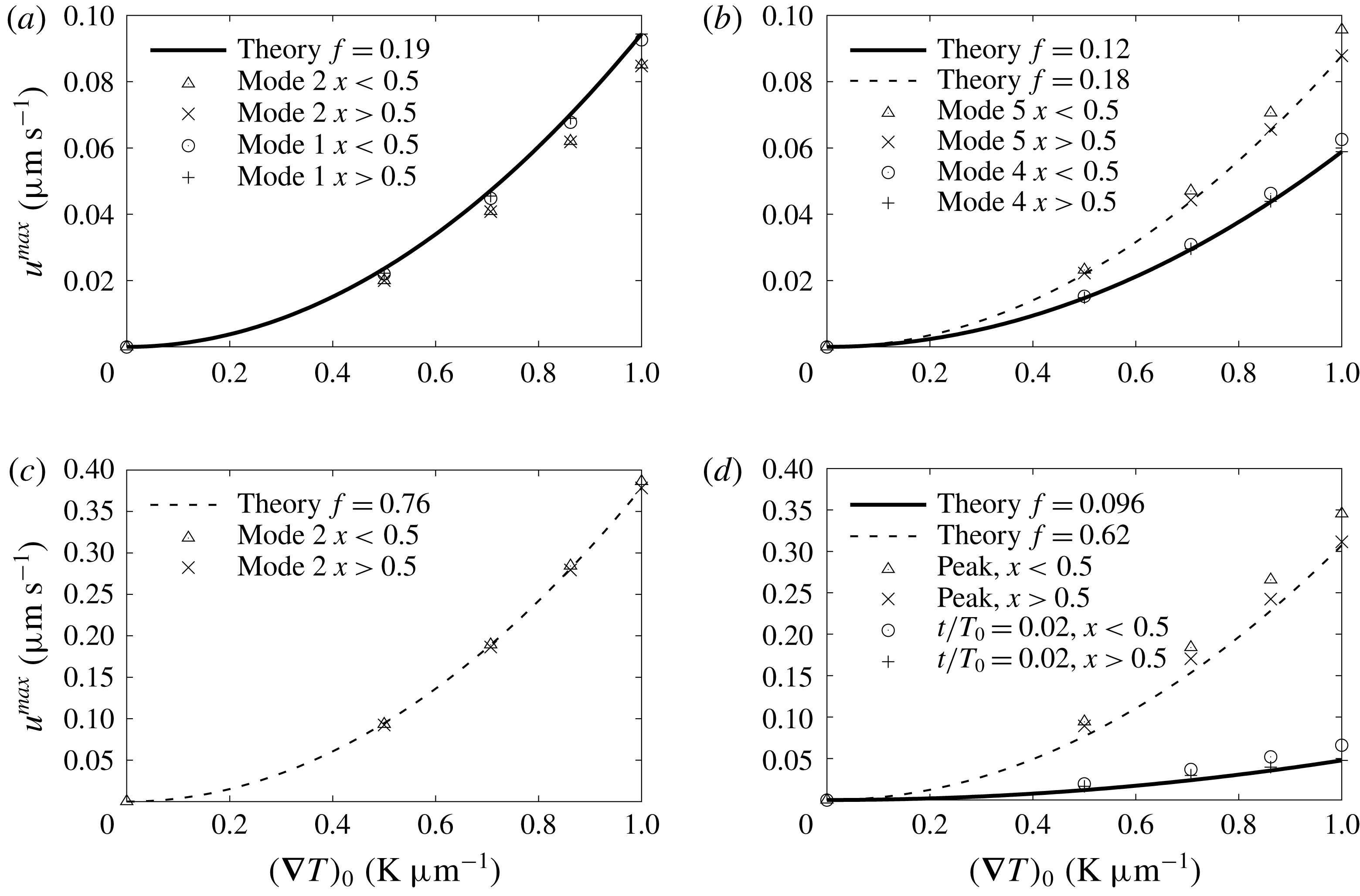
Figure 5(a,b) shows the dependence of
 $u_{max}$
on
 $(\unicode[STIX]{x1D735}T)_{0}$
for the passing and blocking boundary conditions, respectively. In figure 5(a), solid lines denote the analytical results described by (2.21) with
 $f=0.19$
; i.e. we find that
 $u_{max}\propto (\unicode[STIX]{x1D735}T)_{0}^{2}$
for the passing boundary condition. Further, since the results of the steady state for Modes 1 and 2 agree with each other, we can recognize that the difference of the initial stage does not affect the steady state under the passing boundary condition. In figure 5(b), solid and broken lines denote the theoretical curves described by (2.21) with
 $f=0.12$
and 0.18 for Modes 4 and 5, respectively in the region
 $x>0.5$
; i.e. we also find that
 $u_{max}\propto (\unicode[STIX]{x1D735}T)_{0}^{2}$
under the blocking boundary condition. Further, from figure 5(a,b), we find that the difference of the initial behaviour affects the flow velocities in Modes 4 and 5.
Figure 5(c) shows the NTKP at the peak and the broken line denotes the analytical result described by (2.21) with
 $f=0.76$
. Here, since we theoretically expect
 $f=1$
for an unbounded problem (Sugioka Reference Sugioka2014b
), the values of
 $f(=~0.76)$
are acceptable as the first attempt. Figure 5(d) shows the NTKP of Mode 3 and the solid and broken lines denote the analytical results described by (2.21) with
 $f=0.096$
and 0.62, respectively. i.e. we also find that approximately
 $u^{max}\propto (\unicode[STIX]{x1D735}T)_{0}^{2}$
for Mode 3. However, in detail, the numerical results of Mode 3 are slightly different from the relation [
 $u^{max}\propto (\unicode[STIX]{x1D735}T)_{0}^{2}$
] because of the consideration of the temperature dependences of the parameters.
3.5 Two kinds of NTKP relevant to the passing and blocking boundary conditions
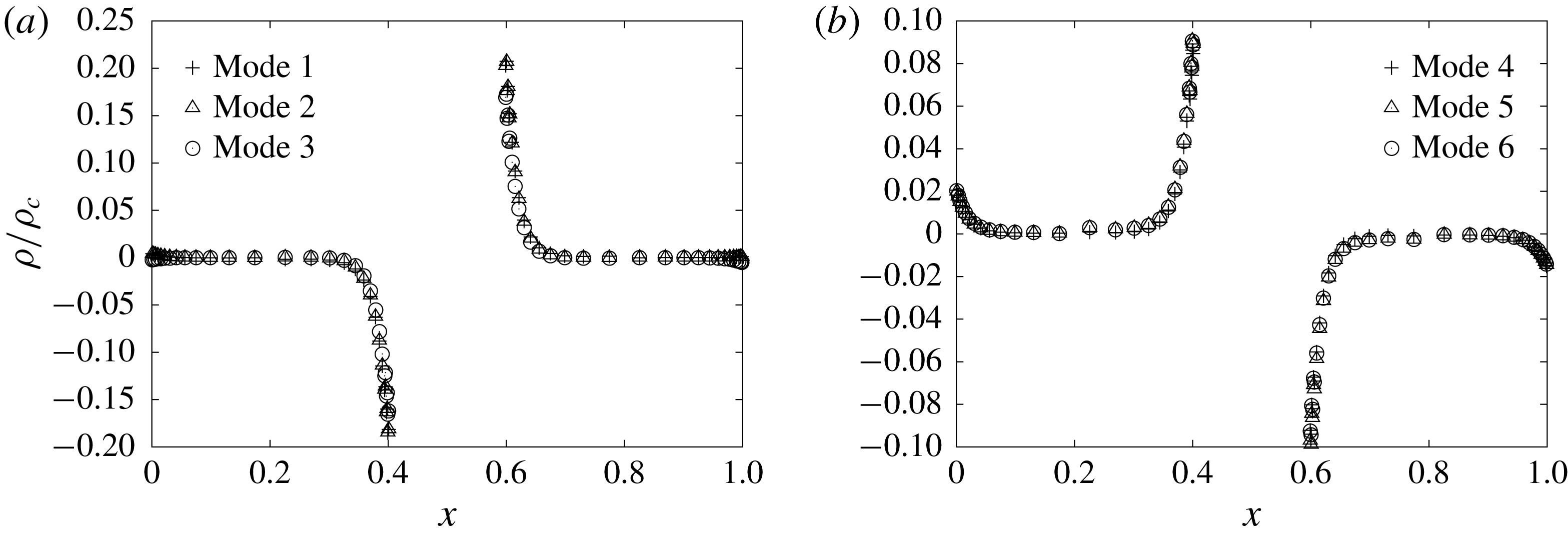
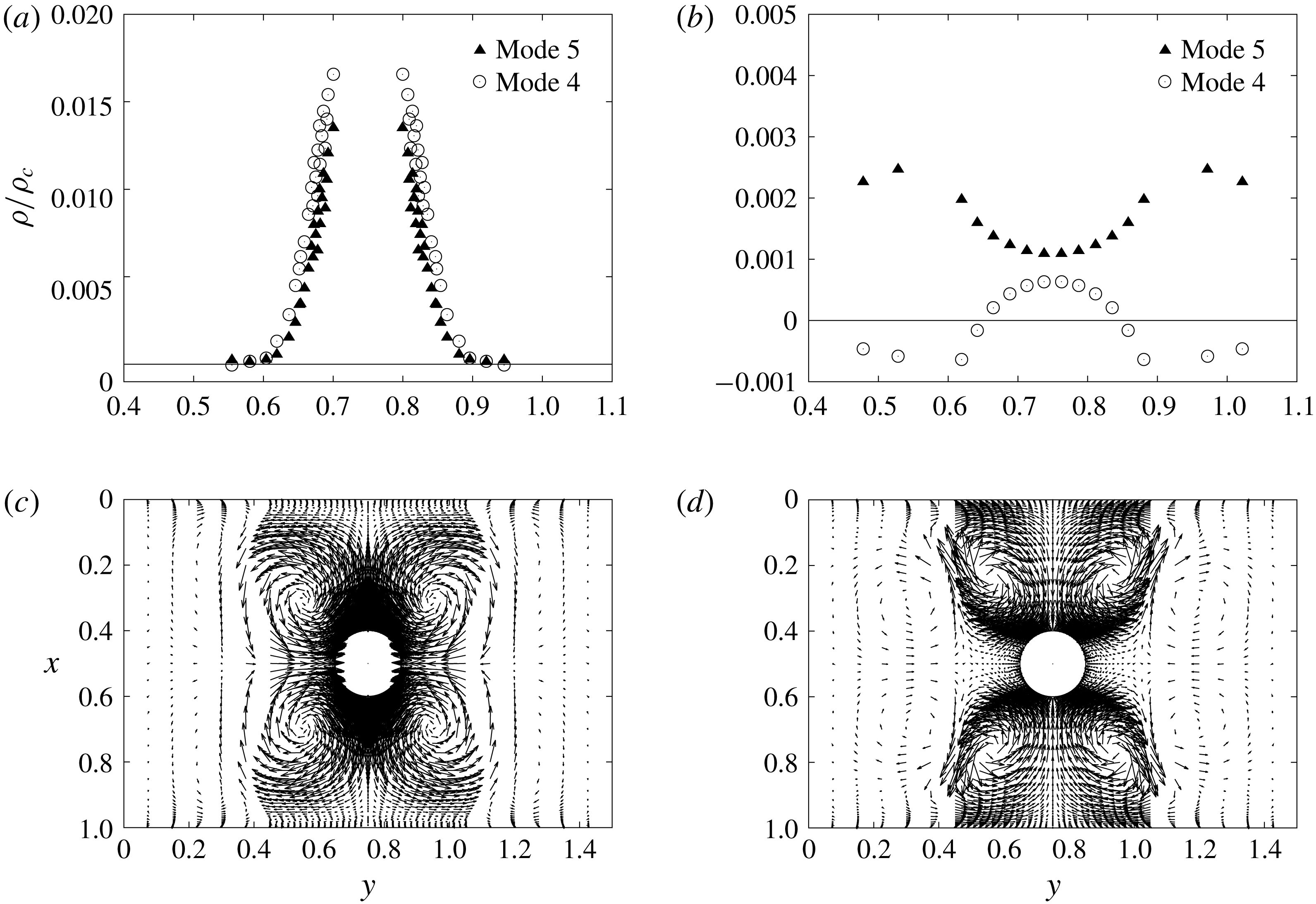
Figure 6(a,b) shows the dependence of
 $\unicode[STIX]{x1D70C}$
on
 $x$
at
 $y=0.75$
for the passing and blocking boundary conditions, respectively. From figure 6, we find that the sign of the charge around the metal cylinder for the blocking boundary condition is the opposite to that for the passing boundary condition. In other words, figure 6 clearly shows that there exist two kinds of NTKP corresponding to the passing and blocking boundary conditions; i.e. the Seebeck effect (SE) type NTKP and the image effect (IE) type NTKP. Here, the image (charge) effect is a kind of induced-charge phenomenon of metal and the IE-NTKP is approximately explained by the primitive model in figure 1. Further, SE-NTKP is the NTKP that is generated by the electric field in the
 $x$
direction due to the Seebeck effect (
 $\boldsymbol{E}^{Seebeck}$
); thus, because of the polarization of the metal cylinder, the sign of the net ion charge at
 $x\simeq 0.4$
and 0.6 becomes positive and negative, as shown in figure 6(b). Note that in IE-NTKP, the charge on the metal is induced through the image effect by the existence of the charge around the metal cylinder, whereas it is induced by the electric field due to the charge near the wall in SE-NTKP.
Dependence of
 $\unicode[STIX]{x1D70C}_{n}$
on
 $x$
at
 $y=0.75$
at
 $t/T_{0}=0.01$
. (a,b) Show the different origins of the NTKP due to the boundary conditions. (a) Value of
 $\unicode[STIX]{x1D70C}$
for the passing BC (b) Value of
 $\unicode[STIX]{x1D70C}$
for the blocking BC.

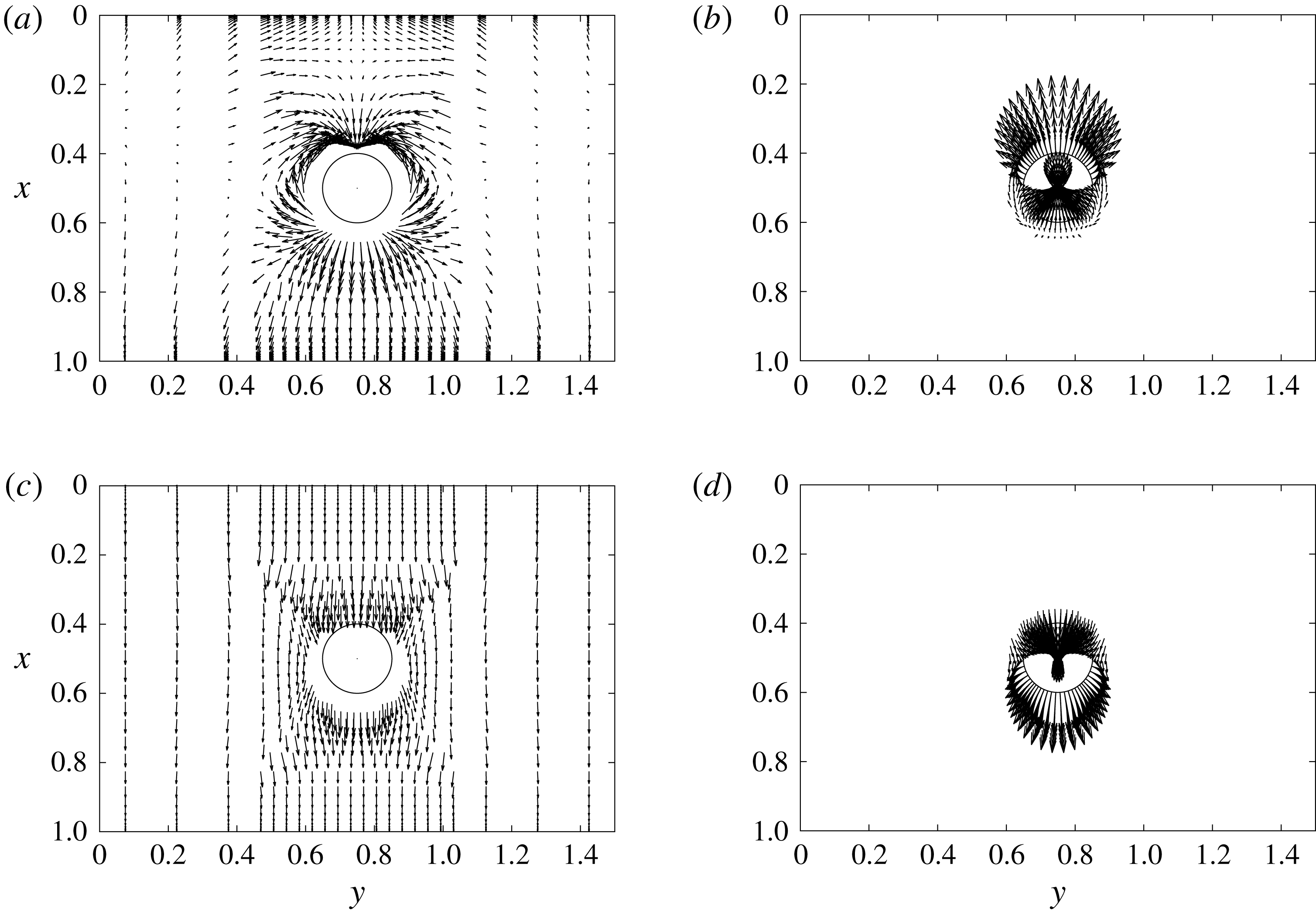
Figure 7 shows the outside and inside electric fields in Modes 3 and 6. In figure 7(b,d), the direction of the inside electric field in Mode 3 (i.e. IE-NTKP) is opposite to that in Mode 6 (i.e. SE-NTKP). On the one hand, in IE-NTKP (Mode 3), the charge around the metal cylinder dominates the phenomena. Thus, the electric field in
 $|\boldsymbol{r}|>1.5a$
is much smaller than that in
 $|\boldsymbol{r}|<1.5a$
in figure 7(a,b). Further, by considering positive and negative charges at
 $x\simeq 0.6$
and 0.4, we can understand that the direction of the electric fields is reasonable; e.g. the circular electric field from
 $x\simeq 0.6$
to
 $x\simeq 0.4$
is explained in figure 7(a,b). On the other hand, in SE-NTKP (Mode 6), the charge near the wall dominates the phenomena. Thus, the electric field in
 $|\boldsymbol{r}|>1.5a$
is similar to that in
 $|\boldsymbol{r}|<1.5a$
in figure 7(c,d). Further, the direction of the outside and inside electric fields are simply explained by considering the existence of positive and negative charges at
 $x\simeq 0$
and 1.
Outside and inside electric fields in Modes 3 and 6. (a) Outside electric field in Mode 3 at
 $t/T_{0}=0.01$
(
 $|\boldsymbol{r}|>1.5a$
,
 $f^{\prime \prime }=10$
). (b) Inside electric field in Mode 3 at
 $t/T_{0}=0.01$
(
 $|\boldsymbol{r}|<1.5a$
,
 $f^{\prime \prime }=2$
). (c) Outside electric field in Mode 6 at
 $t/T_{0}=0.002$
(
 $|\boldsymbol{r}|>1.5a$
,
 $f^{\prime \prime }=2$
). (d) Inside electric field in Mode 6 at
 $t/T_{0}=0.002$
(
 $|\boldsymbol{r}|<1.5a$
,
 $f^{\prime \prime }=2$
).

3.6 Memory and non-steady effects
Time dependence of
 $u^{max}$
(memory and non-steady effects). (a) Modes 1 and 2 (passing BC). (b) Modes 2 and 3 (passing BC). (c) Modes 4 and 5 (blocking BC). (d) Modes 5 and 6 (blocking BC).

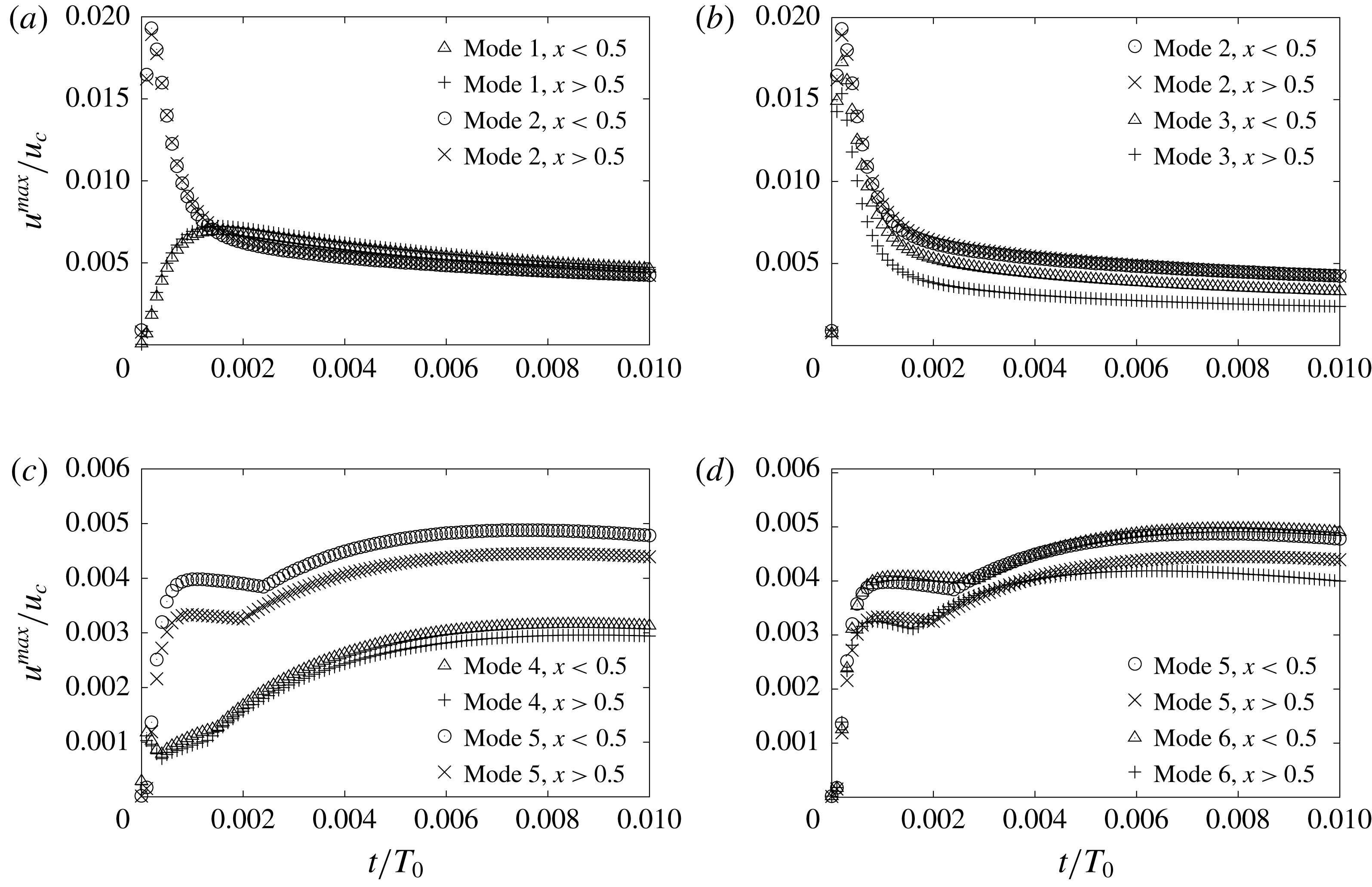
Figure 8 shows the time dependence of
 $u^{max}$
. In figure 8(a), we find a large peak of
 $u^{max,peak}\simeq 0.02$
due to the non-steady effect of Mode 2. Further, we find that the non-steady temperature effect disappears at approximately
 $t/T_{0}>0.002$
and
 $u^{max}$
becomes almost the same for Modes 1 and 2. Further, because of the effect of the temperature dependence of
 $\unicode[STIX]{x1D707}$
and
 $D_{\pm }$
,
 $u^{max,peak}$
in Mode 3 becomes
 $11$
–17% smaller than that in Mode 2, as shown in figure 8(b), although the time-dependent behaviours are almost the same qualitatively. Further, in figure 8(c), we find a significant memory effect in Modes 4 and 5; i.e. the difference of
 $u^{max}$
during the transient state affects the flow velocity of the steady state under the blocking boundary condition (in figure 8
c), whereas the difference in the transient state does not affect the flow velocity of the steady state under the passing ion condition (in figure 8
a). In addition, in figure 8(d), the time-dependent behaviours are almost the same in Modes 5 and 6; i.e. the effect using the temperature dependence of the parameter is rather small for the blocking boundary condition.
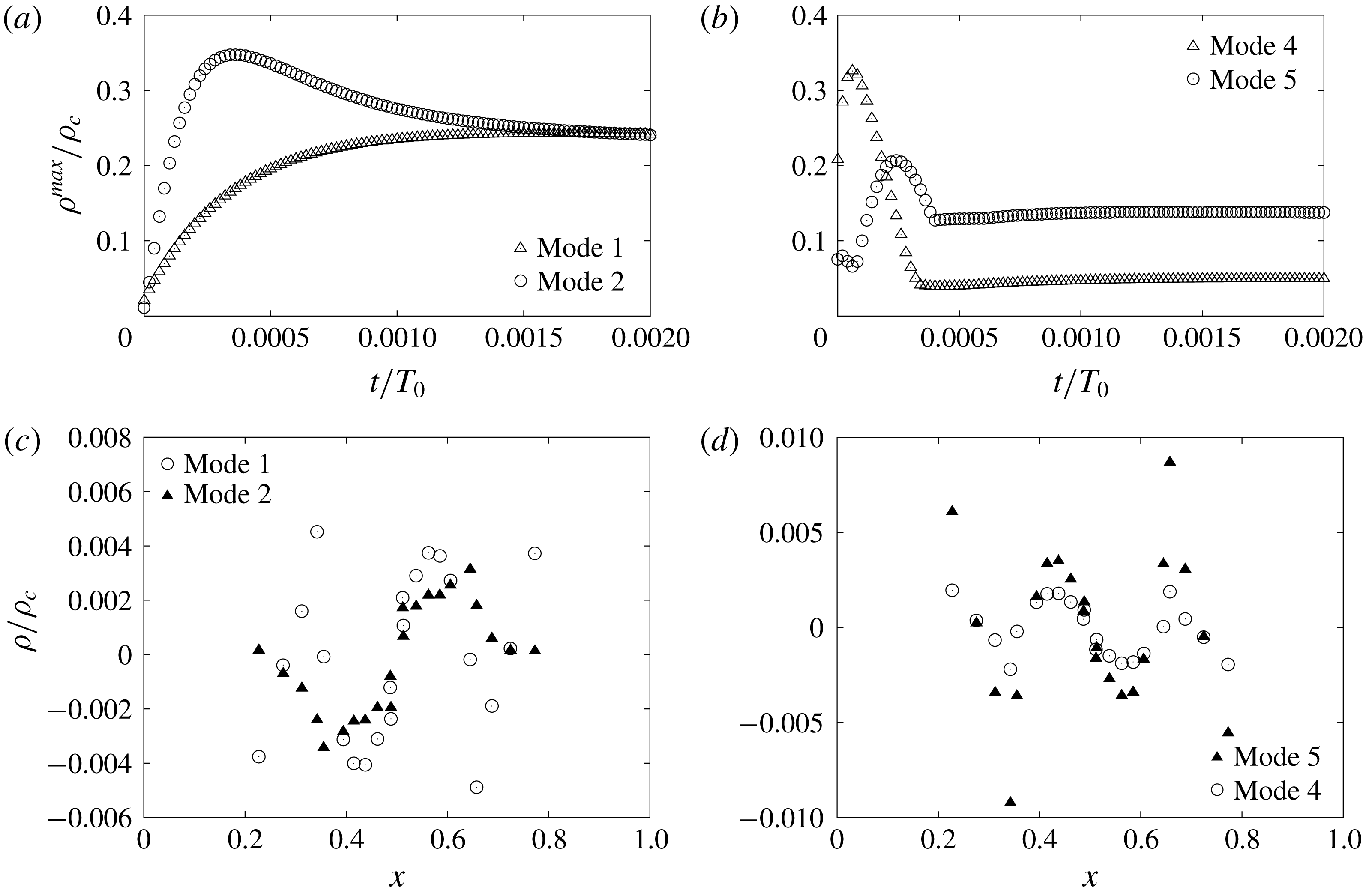
Figure 9(a,b) shows the time evolution the maximum value of
 $\unicode[STIX]{x1D70C}$
(i.e.
 $\unicode[STIX]{x1D70C}^{max}$
) at
 $x>0.5$
. We find that the memory effect for
 $\unicode[STIX]{x1D70C}^{max}$
exists for the blocking boundary condition, whereas it does not exist for the passing boundary condition. Further, figure 9(c,d) shows the dependence of
 $\unicode[STIX]{x1D70C}$
on
 $x$
at
 $y=0.6$
and
 $t/T_{0}=0.01$
. In figure 9(d), we find that a significant difference of
 $\unicode[STIX]{x1D70C}$
exists between Modes 4 and 5, whereas the difference of
 $\unicode[STIX]{x1D70C}$
is rather small between Modes 1 and 2 in figure 9(c). Note that the dependence of
 $\unicode[STIX]{x1D70C}$
on
 $x$
at
 $y=0.75$
(i.e. at the mid-position) for Mode 5 is the same as that for Mode 4 at
 $t/T=0.01$
, as shown in figure 6(b); thus, we consider that the hysteresis of
 $\unicode[STIX]{x1D70C}$
(in figure 9
b,d) causes the memory effect of Modes 4–6.
The time evolution of
 $\unicode[STIX]{x1D70C}^{max}$
at
 $x>0.5$
and the dependence of
 $\unicode[STIX]{x1D70C}$
on
 $x$
at
 $t/T_{0}=0.01$
. (a)
 $\unicode[STIX]{x1D70C}$
for the passing BC (
 $x>0.5$
). (b)
 $\unicode[STIX]{x1D70C}$
for the blocking BC (
 $x>0.5$
). (c)
 $\unicode[STIX]{x1D70C}$
for the passing BC (
 $y=0.6$
). (d)
 $\unicode[STIX]{x1D70C}$
for the blocking BC (
 $y=0.6$
).

3.7 Time evolution of the ion distributions in Modes 3 and 6
Time evolution of the ion distributions in Mode 3 (IE-NTKP). (a) Dependence of
 $C_{+}$
on
 $x$
at
 $y=0.75$
. (b) Dependence of
 $C_{-}$
on
 $x$
at
 $y=0.75$
. (c) Dependence of
 $\unicode[STIX]{x1D70C}_{e}$
on
 $x$
at
 $y=0.75$
. (d) Dependence of
 $\unicode[STIX]{x1D719}$
on
 $x$
at
 $y=0.75$
.

Time evolution of the ion distributions in Mode 6 (SE-NTKP). (a) Dependence of
 $C_{+}$
on
 $x$
at
 $y=0.75$
. (b) Dependence of
 $C_{-}$
on
 $x$
at
 $y=0.75$
. (c) Dependence of
 $\unicode[STIX]{x1D70C}_{e}$
on
 $x$
at
 $y=0.75$
. (d) Dependence of
 $\unicode[STIX]{x1D719}$
on
 $x$
at
 $y=0.75$
.

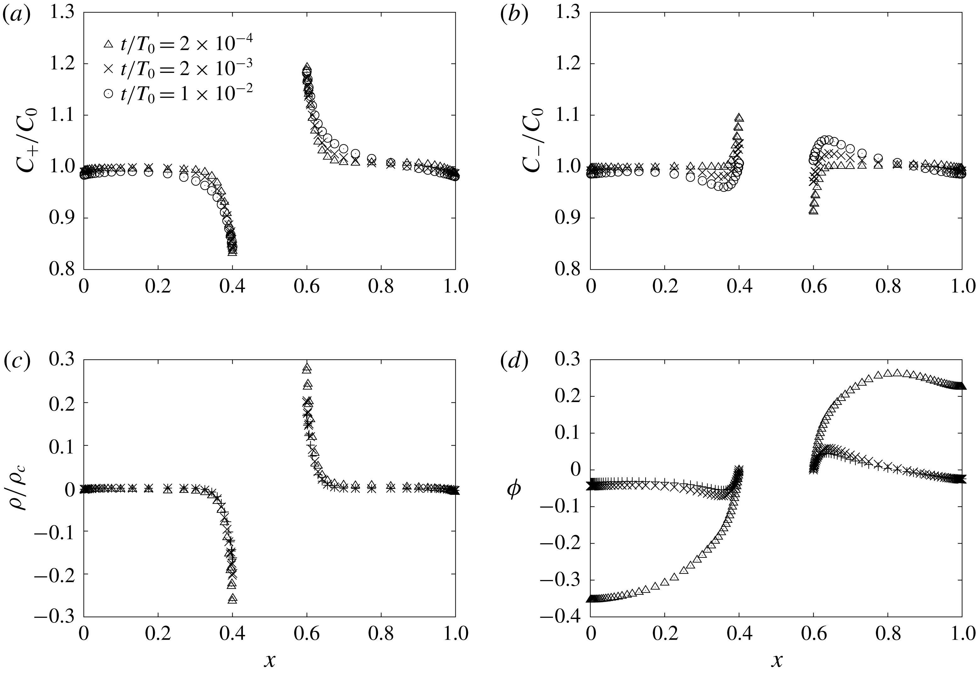
Figure 10 shows the dependence of
 $C_{+}$
,
 $C_{-}$
,
 $\unicode[STIX]{x1D70C}$
and
 $\unicode[STIX]{x1D719}$
on
 $x$
at
 $y=0.75$
at
 $t/T_{0}=0.0002$
, 0.002 and 0.01 in Mode 3. Since the thermal mobility factor of H
 $^{+}$
(
 $2\unicode[STIX]{x1D6FC}_{+}D_{+}=49.6D_{0}$
) is much larger than that of
 $\text{Cl}^{-}$
(
 $2\unicode[STIX]{x1D6FC}_{-}D_{-}=0.431D_{0}$
) (Agar et al.
Reference Agar, Mou and Long Lin1989; Majee & Würger Reference Majee and Würger2012), the positive ion (H
 $^{+}$
) moves from a hotter region to a colder region with a much faster velocity than the negative ion (
 $\text{Cl}^{-}$
). Thus, in figure 10(a,b),
 $C_{+}$
becomes much larger than
 $C_{-}$
at
 $x\simeq 0.6$
whereas
 $C_{-}$
becomes much larger than
 $C_{+}$
at
 $x\simeq 0.4$
. Consequently, in figure 10(c), we can observe a positive charge region at the hotter side of the metal cylinder, whereas we can observe a negative charge region at the colder side. In detail, the time evolution of
 $C_{-}$
around the metal cylinder (in figure 10
b) is complex and it should be explained by the image charge effect of the positive ion (H
 $^{+}$
). Further, we find that the arrival of the fast ion in the initial stage (at
 $t/T_{0}=0.0002$
) induces a large transient charge density around the metal through the image charge effect and a large electric field in the
 $-x$
direction, whereas the arrival of the slow ion in the final stage (at
 $t/T_{0}=0.01$
) suppresses the charge and the electric field around the metal. This is the reason why
 $u^{max}$
in Modes 2 and 3 is large in the initial stage and suppressed in the final stage (in figure 8
b). Note that in Mode 3, the concentrations of ions at the edges are almost the same as the bulk concentration (in figure 10
a,b) and the charges at the edges are almost zero (in figure 10
c).
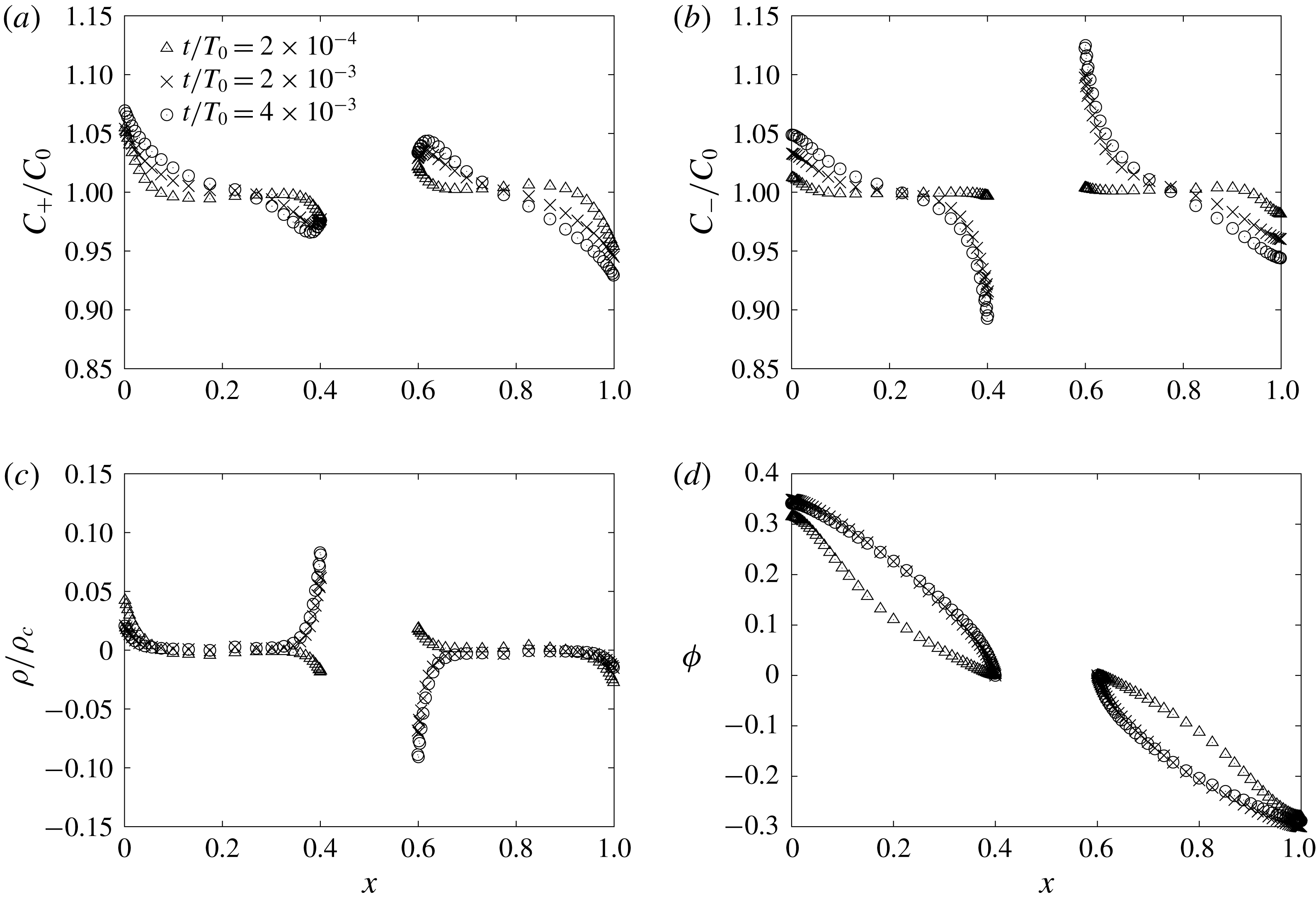
Figure 11 shows the dependences of
 $C_{+}$
,
 $C_{-}$
,
 $\unicode[STIX]{x1D70C}$
and
 $\unicode[STIX]{x1D719}$
on
 $x$
at
 $y=0.75$
at
 $t/T_{0}=0.0002$
, 0.002 and 0.01 in Mode 6. Since ions cannot go through the edges in Mode 6, the concentration of ions at the colder (hotter) edge is larger (smaller) than the bulk concentration (in figure 11
a,b) and the charge at the colder (hotter) edge becomes positive (negative) in Mode 6 (in figure 11
c). As a result, the potential difference between the edges becomes large in Mode 6 (in figure 11
d). Thus, the large electric field in the
 $x$
direction is generated through the Seebeck effect and it drives ICEO phenomena around the metal.
4 Discussion
4.1 The gradient of ion concentration for the blocking boundary condition at the wall
If we can neglect the effect of the charge of ions, we can estimate the gradient of ion concentrations due to thermokinetic phenomena for the blocking boundary condition by using (2.8) and (2.13) as follows:
 $$\begin{eqnarray}\displaystyle & \displaystyle \unicode[STIX]{x1D735}_{n}c_{+}=-2\frac{\unicode[STIX]{x1D6FC}_{+}}{\tilde{T}}c_{+}\frac{\unicode[STIX]{x1D735}_{n}\tilde{T}}{\tilde{T}}\simeq -2\unicode[STIX]{x1D6FC}_{+}(\unicode[STIX]{x1D735}_{n}\tilde{T})_{0}, & \displaystyle\end{eqnarray}$$
 $$\begin{eqnarray}\displaystyle & \displaystyle \unicode[STIX]{x1D735}_{n}c_{-}=-2\frac{\unicode[STIX]{x1D6FC}_{-}}{\tilde{T}}c_{-}\frac{\unicode[STIX]{x1D735}_{n}\tilde{T}}{\tilde{T}}\simeq -2\unicode[STIX]{x1D6FC}_{-}(\unicode[STIX]{x1D735}_{n}\tilde{T})_{0}, & \displaystyle\end{eqnarray}$$
where
 $\unicode[STIX]{x1D6FC}_{+}\simeq 2.7$
(for H
 $^{+}$
),
 $\unicode[STIX]{x1D6FC}_{-}\simeq 0.1$
(for Cl
 $^{-}$
),
 $\unicode[STIX]{x1D735}_{n}\tilde{T}\simeq (\unicode[STIX]{x1D735}_{n}\tilde{T})_{0}[=(1~\text{K}/1~\unicode[STIX]{x03BC}\text{m})\times (50~\unicode[STIX]{x03BC}\text{m}/300~\text{K})=0.167]$
,
 $\tilde{T}\simeq 1$
and
 $c_{\pm }\simeq 1$
. That is,
 $\unicode[STIX]{x1D735}_{n}c_{+}\gg \unicode[STIX]{x1D735}_{n}c_{-}$
in the first stage and the tendencies toward
 $\unicode[STIX]{x1D735}_{n}c_{+}\simeq -2\times 2.7\times 0.167\simeq -0.9$
and
 $\unicode[STIX]{x1D735}_{n}c_{-}-2\times 0.1\times 0.167\simeq -0.03$
are the basic driving forces of the phenomenon. However, since the difference of
 $\unicode[STIX]{x1D735}_{n}c_{\pm }$
produces a net space charge, we need to consider the effect of the electric field on the ion distributions. Namely, by using the numerical result
 $(\unicode[STIX]{x1D735}_{n}\unicode[STIX]{x1D719})_{c}\simeq -0.6$
in figure 11(d), we can estimate as follows:
 $$\begin{eqnarray}\displaystyle \unicode[STIX]{x1D735}_{n}c_{+}=-2\frac{\unicode[STIX]{x1D6FC}_{+}}{\tilde{T}}c_{+}\frac{\unicode[STIX]{x1D735}_{n}\tilde{T}}{\tilde{T}}-c_{\pm }\frac{\unicode[STIX]{x1D735}_{n}\unicode[STIX]{x1D719}}{\tilde{T}}\simeq -2\unicode[STIX]{x1D6FC}_{+}(\unicode[STIX]{x1D735}_{n}\tilde{T})_{0}-(\unicode[STIX]{x1D735}_{n}\unicode[STIX]{x1D719})_{c}. & & \displaystyle\end{eqnarray}$$
Since the numerical value of
 $\unicode[STIX]{x1D735}_{n}c_{+}$
is approximately
 $-0.35~(\simeq -0.07/0.2)$
in figure 11(a), the estimation (
 $\unicode[STIX]{x1D735}_{n}c_{+}\simeq -2\times 2.7\times 0.167+0.6\simeq -0.3$
) of (4.3) is reasonable. Note that the generation of an electric field due to thermophoresis also affects
 $\unicode[STIX]{x1D735}_{n}c_{-}$
and it increases the gradient of
 $c_{-}$
. Thus,
 $\unicode[STIX]{x1D735}_{n}c_{-}$
takes a value similar to
 $\unicode[STIX]{x1D735}_{n}c_{+}$
in the bulk region and the existence of charge is limited in the wall region of thickness approximately
 $\unicode[STIX]{x1D706}_{D}$
, as shown in figure 11(a–c). Usually, this process is simply explained by the Seebeck effect described by (2.24), which is derived from (2.8) under the zero current condition and the assumption
 $c_{+}\simeq c_{-}$
in the bulk region. Thus,
 $\unicode[STIX]{x1D735}_{n}\unicode[STIX]{x1D719}$
can be estimated by (2.24). For instance, since
 $S_{e}=374~\unicode[STIX]{x03BC}\text{V}~\text{K}^{-1}$
for a HCl solution, the potential difference
 $\unicode[STIX]{x0394}\unicode[STIX]{x1D719}=-374\times 50\simeq -18.7$
mV (
 $-0.72\unicode[STIX]{x1D6F7}_{c}$
) for
 $W=50~\unicode[STIX]{x03BC}\text{m}$
; thus, we obtain
 $\unicode[STIX]{x1D735}_{n}\unicode[STIX]{x1D719}\simeq -0.72$
, which approximately agrees with the result of figure 11(d) (i.e.
 $\unicode[STIX]{x1D735}_{n}\unicode[STIX]{x1D719}\simeq -0.6$
and
 $\unicode[STIX]{x0394}\unicode[STIX]{x1D719}\simeq 0.6$
), where
 $\unicode[STIX]{x1D6F7}_{c}=kT_{a}/ze=25.9$
mV.
4.2 The influence of the electrolyte concentration near the wall
Since
 $\unicode[STIX]{x1D706}_{D}\equiv \sqrt{\unicode[STIX]{x1D700}kT_{a}/2z^{2}e^{2}C_{0}}$
,
 $\unicode[STIX]{x1D706}_{D}$
decreases as
 $C_{0}$
increases. As discussed in § 4.1, for the blocking boundary condition,
 $c_{\pm }$
(and
 $\unicode[STIX]{x1D735}_{n}c_{\pm }$
) takes the same value except in the wall region of thickness
 $\unicode[STIX]{x1D706}_{D}$
because of the interaction between the positive and negative ions with the screening effect of the electric field. Moreover, in our understanding,
 $\unicode[STIX]{x1D735}_{n}c_{+}$
and
 $\unicode[STIX]{x1D735}_{n}c_{-}$
near the wall region are approximated by the maximum gradient of
 $c_{+}$
of (4.1) and zero, respectively; i.e.
 $\unicode[STIX]{x1D735}_{n}c_{+}^{wall}\simeq -0.9$
and
 $\unicode[STIX]{x1D735}_{n}c_{-}^{wall}\simeq 0$
. Thus, we estimate the maximum charge density near the wall as
 $$\begin{eqnarray}\displaystyle \unicode[STIX]{x1D70C}^{wall}/\unicode[STIX]{x1D70C}_{c}\simeq |\unicode[STIX]{x1D735}_{n}c_{+}^{wall}|\frac{\unicode[STIX]{x1D706}_{D}}{W}\simeq |2\unicode[STIX]{x1D6FC}_{+}(\unicode[STIX]{x1D735}_{n}\tilde{T})_{0}|\frac{\unicode[STIX]{x1D706}_{D}}{W}, & & \displaystyle\end{eqnarray}$$
where
 $|2\unicode[STIX]{x1D6FC}_{+}(\unicode[STIX]{x1D735}_{n}\tilde{T})_{0}|\simeq 0.9$
,
 $\unicode[STIX]{x1D706}_{D}=1~\unicode[STIX]{x03BC}\text{m}$
, and
 $W=50~\unicode[STIX]{x03BC}\text{m}$
; i.e.
 $\unicode[STIX]{x1D70C}^{wall}/\unicode[STIX]{x1D70C}_{c}\simeq 0.02$
. Since the numerical result of
 $\unicode[STIX]{x1D70C}^{wall}/\unicode[STIX]{x1D70C}_{c}$
at
 $x=0$
for the steady state in figure 11(c) is also
 $\simeq 0.02$
, our simple argument of (4.4) explains the thermokinetic phenomena near the wall to some extent.
Further, the charge per unit area near the wall is written as
 $\unicode[STIX]{x1D70E}^{wall}=\unicode[STIX]{x1D70C}^{wall}\unicode[STIX]{x1D706}_{D}$
. Thus, the electric field produced by the charge near the wall in SE-NTKP is described as
 $$\begin{eqnarray}\displaystyle E_{se(1)}\simeq \frac{\unicode[STIX]{x1D70C}^{wall}\unicode[STIX]{x1D706}_{D}}{\unicode[STIX]{x1D700}}\simeq 2\unicode[STIX]{x1D6FC}_{+}(\unicode[STIX]{x1D735}_{n}\tilde{T})_{0}\frac{\unicode[STIX]{x1D706}_{D}^{2}}{W\unicode[STIX]{x1D700}}\unicode[STIX]{x1D70C}_{c}. & & \displaystyle\end{eqnarray}$$
Namely, for the current condition, we obtain
 $E_{se(1)}=245.7~\text{V}~\text{m}^{-1}$
and find that the potential difference across the chamber is
 $\unicode[STIX]{x0394}\unicode[STIX]{x1D6F7}=E_{se(1)}W=12.3$
mV (
 ${\sim}0.5\unicode[STIX]{x1D6F7}_{c}$
). Since this approximately agrees with the numerical result of
 $\unicode[STIX]{x0394}\unicode[STIX]{x1D6F7}\simeq 0.6\unicode[STIX]{x1D6F7}_{c}$
in figure 11(d), equation (4.5) is reasonable. Consequently, according to our argument, we can understand that
 $E_{se(1)}$
and
 $\unicode[STIX]{x1D70E}^{wall}$
does not change even if
 $C_{0}$
changes, although
 $\unicode[STIX]{x1D70C}^{wall}$
is proportional to
 $\sqrt{C_{0}}$
.
4.3 The gradient of ion concentration around the metal cylinder in IE-NTKP
From (2.1), we obtain
 $$\begin{eqnarray}\frac{\unicode[STIX]{x2202}T}{\unicode[STIX]{x2202}r}\simeq \left(1+\frac{a^{2}}{r^{2}}\right)(\unicode[STIX]{x1D735}T)_{0}\cos \unicode[STIX]{x1D703}.\end{eqnarray}$$
Thus, we can approximate that
 $\unicode[STIX]{x1D735}_{n}\tilde{T}\simeq 2(\unicode[STIX]{x1D735}_{n}\tilde{T})_{0}=0.334$
at
 $x=0.4$
and 0.6. Therefore, by using a similar argument to that in § 4.1, if we can neglect the charge of the particles and the image effect of the metal, we can estimate the gradient of ions around the metal as follows:
 $$\begin{eqnarray}\displaystyle & \displaystyle \unicode[STIX]{x1D735}_{n}c_{+}^{metal}\simeq -4\unicode[STIX]{x1D6FC}_{+}(\unicode[STIX]{x1D735}_{n}\tilde{T})_{0}, & \displaystyle\end{eqnarray}$$
 $$\begin{eqnarray}\displaystyle & \displaystyle \unicode[STIX]{x1D735}_{n}c_{-}^{metal}\simeq -4\unicode[STIX]{x1D6FC}_{-}(\unicode[STIX]{x1D735}_{n}\tilde{T})_{0}. & \displaystyle\end{eqnarray}$$
That is, the tendencies toward
 $\unicode[STIX]{x1D735}_{n}c_{+}^{metal}\simeq -1.8$
and
 $\unicode[STIX]{x1D735}_{n}c_{-}^{metal}\simeq -0.06$
are the basic driving forces of the phenomenon around the metal cylinder. Different from the argument of § 4.1, as a first step we can neglect the second term of (4.3) because of the existence of the image charge of the metal cylinder. Further, since
 $\unicode[STIX]{x1D735}_{n}c_{+}\simeq -0.2/0.1\simeq -2$
at
 $x\simeq 0.4$
and 0.6 in figure 10(a), the estimation of (4.7) is reasonable. Similar to the discussion in §§ 4.1 and 4.2,
 $c_{\pm }$
(and
 $\unicode[STIX]{x1D735}_{n}c_{\pm }$
) takes the same value except in the surrounding region of the metal cylinder of thickness
 $\unicode[STIX]{x1D706}_{D}$
because of the interaction between the positive and negative ions with the screening effect of the electric field. However, because of the existence of the image charge of the metal cylinder, the maximum charge density near the metal cylinder becomes twice that near the unpolarizable wall:
 $$\begin{eqnarray}\displaystyle \unicode[STIX]{x1D70C}_{ie.m(1)}/\unicode[STIX]{x1D70C}_{c}\simeq 8\unicode[STIX]{x1D6FC}_{+}(\unicode[STIX]{x1D735}_{n}\tilde{T})_{0}\frac{\unicode[STIX]{x1D706}_{D}}{W}. & & \displaystyle\end{eqnarray}$$
In fact, different from
 $c_{-}$
at
 $x\simeq 0.6$
in figure 11(b),
 $c_{-}$
at
 $x\simeq 0.6$
in figure 10(b) decreases as the position approaches the surface of the metal because of the image effect and thus the charge increases rapidly near the metal. In addition, because of the polarization effect of the metal due to the existence of the excess counter-ions at the other side, the maximum charge density becomes twice again with respect to the left side value of (4.9); i.e.
 $$\begin{eqnarray}\displaystyle \unicode[STIX]{x1D70C}_{ie.m(2)}/\unicode[STIX]{x1D70C}_{c}\simeq 16\unicode[STIX]{x1D6FC}_{+}(\unicode[STIX]{x1D735}_{n}\tilde{T})_{0}\frac{\unicode[STIX]{x1D706}_{D}}{W}. & & \displaystyle\end{eqnarray}$$
Since
 $\unicode[STIX]{x1D70C}_{ie.m(2)}/\unicode[STIX]{x1D70C}_{c}\simeq 0.014$
, the numerical result of
 $\unicode[STIX]{x1D70C}/\unicode[STIX]{x1D70C}_{c}\sim 0.2$
at
 $x\simeq 0.6$
in figure 10(c) is approximately explained by our simple argument. Further, since
 $\unicode[STIX]{x1D70C}_{ie.m(2)}\unicode[STIX]{x1D706}_{D}$
represents the charge per unit area at the hotter side of the metal, we can estimate the zeta potential at
 $x\simeq 0.6$
in IE-NTKP as
 $$\begin{eqnarray}\displaystyle \unicode[STIX]{x1D701}_{ie}^{\prime }\simeq \frac{\unicode[STIX]{x1D706}_{D}^{2}}{\unicode[STIX]{x1D700}}\unicode[STIX]{x1D70C}_{ie.m(2)}\simeq 16\unicode[STIX]{x1D6FC}_{+}(\unicode[STIX]{x1D735}_{n}\tilde{T})_{0}\frac{\unicode[STIX]{x1D706}_{D}^{3}\unicode[STIX]{x1D70C}_{c}}{\unicode[STIX]{x1D700}W}. & & \displaystyle\end{eqnarray}$$
Here,
 $\unicode[STIX]{x1D701}_{ie}^{\prime }$
corresponds to the peak value of
 $\unicode[STIX]{x1D719}$
(
 $\simeq 0.07$
) at
 $x\simeq 0.6$
in figure 10(d); thus,
 $\unicode[STIX]{x1D701}_{ie}^{\prime }\simeq 2.0$
mV (
 $0.076\unicode[STIX]{x1D6F7}_{c}$
) in (4.11) explains the peak value to some extent.
4.4 Theory of IE-NTKP
Based on the Smoluchowski formula, we can describe the IE-NTKP flow velocity as
 $$\begin{eqnarray}\displaystyle u_{ie}^{slip}=\frac{\unicode[STIX]{x1D700}\unicode[STIX]{x1D701}_{ie}^{\prime \prime }}{\unicode[STIX]{x1D707}}E_{ie}, & & \displaystyle\end{eqnarray}$$
where
 $E_{ie}$
denotes an apparent external electric field in IE-NTKP, which acts on the charge in the electric double layer around the metal cylinder, and
 $\unicode[STIX]{x1D701}_{ie}^{\prime \prime }$
is a zeta potential around the metal at the
 $\unicode[STIX]{x1D703}=45^{\circ }$
in IE-NTKP. Since
 $\unicode[STIX]{x1D701}\propto \cos \unicode[STIX]{x1D703}$
around the metal cylinder, we can approximate
 $$\begin{eqnarray}\displaystyle \unicode[STIX]{x1D701}_{ie}^{\prime \prime }\simeq \frac{\unicode[STIX]{x1D701}_{ie}^{\prime }}{\sqrt{2}}\simeq 8\sqrt{2}\unicode[STIX]{x1D6FC}_{+}(\unicode[STIX]{x1D735}_{n}\tilde{T})_{0}\frac{\unicode[STIX]{x1D706}_{D}^{3}\unicode[STIX]{x1D70C}_{c}}{\unicode[STIX]{x1D700}W}. & & \displaystyle\end{eqnarray}$$
Further, the electric field in figure 7(a) shows that
 $E_{ie}$
in IE-NTKP should be described as
 $$\begin{eqnarray}\displaystyle E_{ie}\simeq -\frac{2\unicode[STIX]{x1D701}_{ie}^{\prime }}{\unicode[STIX]{x03C0}(a+\unicode[STIX]{x1D706}_{D})}\simeq -32\unicode[STIX]{x1D6FC}_{+}(\unicode[STIX]{x1D735}_{n}\tilde{T})_{0}\frac{\unicode[STIX]{x1D706}_{D}^{3}\unicode[STIX]{x1D70C}_{c}}{\unicode[STIX]{x1D700}W}. & & \displaystyle\end{eqnarray}$$
By substituting (4.13) and (4.14) into (4.12), we obtain
 $$\begin{eqnarray}\displaystyle u_{ie}^{slip}\simeq -\frac{\sqrt{2}\unicode[STIX]{x1D700}{\unicode[STIX]{x1D701}^{\prime }}^{2}}{\unicode[STIX]{x03C0}(a+\unicode[STIX]{x1D706}_{D})\unicode[STIX]{x1D707}}. & & \displaystyle\end{eqnarray}$$
Thus, the numerically observable maximum velocity is provided as
 $$\begin{eqnarray}\displaystyle u_{ie}\simeq \frac{1}{2}u_{ie}^{slip}\simeq -\frac{\unicode[STIX]{x1D700}\left[16\unicode[STIX]{x1D6FC}_{+}(\unicode[STIX]{x1D735}_{n}\tilde{T})_{0}{\displaystyle \frac{\unicode[STIX]{x1D706}_{D}^{3}\unicode[STIX]{x1D70C}_{c}}{\unicode[STIX]{x1D700}W}}\right]^{2}}{\sqrt{2}\unicode[STIX]{x03C0}(a+\unicode[STIX]{x1D706}_{D})\unicode[STIX]{x1D707}}. & & \displaystyle\end{eqnarray}$$
In (4.15) and (4.16), a negative value shows the flow is in the
 $-x$
direction near
 $x\simeq 0.6$
. From (4.13), (4.14) and (4.16), we obtain that
 $\unicode[STIX]{x1D701}_{ie}^{\prime \prime }\simeq 0.054\unicode[STIX]{x1D6F7}_{c}\simeq 1.4$
mV,
 $E_{ie}\simeq -209~\text{V}~\text{m}^{-1}$
and
 $u_{ie}\simeq -0.051u_{c}\simeq -0.10~\unicode[STIX]{x03BC}\text{m}~\text{s}^{-1}$
, under the current conditions. Numerical calculation shows that
 $u^{max}\simeq 0.19u_{ntkp}\simeq 0.094~\unicode[STIX]{x03BC}\text{m}~\text{s}^{-1}$
for IE-NTKP in figure 5(a). Thus, equation (4.16) explains the flow velocity of IE-NTKP reasonably. Consequently, our new theory on IE-NTKP is justified to some extent.
4.5 Theory of SE-NTKP
By the Smoluchowski formula, the SE-NTKP flow velocity is described as
 $$\begin{eqnarray}\displaystyle u_{se}^{slip}=\frac{\unicode[STIX]{x1D700}\unicode[STIX]{x1D701}_{se}^{\prime \prime }}{\unicode[STIX]{x1D707}}E_{se}, & & \displaystyle\end{eqnarray}$$
where
 $E_{se}$
denotes an apparent external electric field in SE-NTKP, which acts on the charge in the electric double layer around the metal cylinder, and
 $\unicode[STIX]{x1D701}_{se}^{\prime \prime }$
is a zeta potential around the metal at the
 $\unicode[STIX]{x1D703}=45^{\circ }$
(
 $x\simeq 0.576$
) in SE-NTKP. Further, SE-NTKP is mainly driven by the charge near the wall and thus, on the basis of ICEO theory, the zeta potential due to
 $E^{se(1)}$
(provided by (4.5)) at the hotter side of the metal is described as
 $$\begin{eqnarray}\displaystyle \unicode[STIX]{x1D701}_{se.m(1)}^{\prime }\simeq -2aE_{se(1)}. & & \displaystyle\end{eqnarray}$$
Furthermore, since
 $\unicode[STIX]{x1D70E}=(\unicode[STIX]{x1D700}/\unicode[STIX]{x1D706}_{D})\unicode[STIX]{x1D701}_{se.m(1)}^{\prime }$
, the charge density due to
 $E_{se(1)}$
is described as
 $$\begin{eqnarray}\displaystyle \unicode[STIX]{x1D70C}_{se.m(1)}\simeq -\frac{2aE_{se(1)}\unicode[STIX]{x1D700}}{\unicode[STIX]{x1D706}_{D}^{2}}. & & \displaystyle\end{eqnarray}$$
However, there exists an intrinsic charge density
 $\unicode[STIX]{x1D70C}_{se.m(2)}$
due to the thermophoretic force at the hotter side of the metal in SE-NTKP. That is, similar to the discussion of (4.6) and (4.7), it is described as
 $$\begin{eqnarray}\displaystyle \unicode[STIX]{x1D70C}_{se.m(2)}\simeq 8\unicode[STIX]{x1D6FC}_{+}(\unicode[STIX]{x1D735}_{n}\tilde{T})_{0}\unicode[STIX]{x1D70C}_{c}\frac{\unicode[STIX]{x1D706}_{D}}{W}. & & \displaystyle\end{eqnarray}$$
Note that there are no counter-ions at the other side in SE-NTKP. Thus,
 $\unicode[STIX]{x1D70C}_{se.m(2)}=0.5\unicode[STIX]{x1D70C}_{ie.m(2)}$
. Therefore, by considering the principle of superposition, we obtain a net charge density at the hotter side of the metal in SE-NTKP as
 $$\begin{eqnarray}\displaystyle \unicode[STIX]{x1D70C}_{se.m}\simeq \unicode[STIX]{x1D70C}_{se.m(1)}+\unicode[STIX]{x1D70C}_{se.m(2)}. & & \displaystyle\end{eqnarray}$$
Thus, the corresponding zeta potential is
 $$\begin{eqnarray}\displaystyle \unicode[STIX]{x1D701}_{se}^{\prime }\simeq \frac{\unicode[STIX]{x1D706}_{D}^{2}\unicode[STIX]{x1D70C}_{se.m}}{\unicode[STIX]{x1D700}}. & & \displaystyle\end{eqnarray}$$
As discussed before, we can approximate
 $$\begin{eqnarray}\displaystyle \unicode[STIX]{x1D701}_{se}^{\prime \prime }\simeq \frac{\unicode[STIX]{x1D701}_{se}^{\prime }}{\sqrt{2}}\simeq 2\sqrt{2}\unicode[STIX]{x1D6FC}_{+}(\unicode[STIX]{x1D735}_{n}\tilde{T})_{0}\frac{\unicode[STIX]{x1D706}_{D}^{2}\unicode[STIX]{x1D70C}_{c}}{\unicode[STIX]{x1D700}}\left(-\frac{a}{W}+2\frac{\unicode[STIX]{x1D706}_{D}}{W}\right). & & \displaystyle\end{eqnarray}$$
In addition, by using (4.20), the intrinsic zeta potential around the metal due to
 $\unicode[STIX]{x1D70C}_{se.m(2)}$
is described as
 $$\begin{eqnarray}\displaystyle \unicode[STIX]{x1D701}_{se(2)}^{\prime }\simeq \frac{\unicode[STIX]{x1D706}_{D}^{2}\unicode[STIX]{x1D70C}_{se.m(2)}}{\unicode[STIX]{x1D700}}. & & \displaystyle\end{eqnarray}$$
Thus, the intrinsic electric field
 $E_{se(2)}$
due to
 $\unicode[STIX]{x1D701}_{se.m(2)}^{\prime }$
in SE-NTKP is described as
 $$\begin{eqnarray}\displaystyle E_{se(2)}\simeq -\frac{2\unicode[STIX]{x1D701}_{se(2)}^{\prime }}{\unicode[STIX]{x03C0}(a+\unicode[STIX]{x1D706}_{D})}~\left(=\frac{1}{2}E_{ie}\right). & & \displaystyle\end{eqnarray}$$
Since the electric field outside the electric double layer around the metal at
 $\unicode[STIX]{x1D703}$
is described as
 $E=2E_{0}\sin \unicode[STIX]{x1D703}$
using the external average electric field
 $E_{0}$
in standard ICEO theory (Squires & Bazant Reference Squires and Bazant2004; Sugioka Reference Sugioka2011), we obtain
 $$\begin{eqnarray}\displaystyle E_{se}\simeq 2(E_{se(1)}+E_{se(2)})\sin \frac{\unicode[STIX]{x03C0}}{4}=2\sqrt{2}\unicode[STIX]{x1D6FC}_{+}(\unicode[STIX]{x1D735}_{n}\tilde{T})_{0}\frac{\unicode[STIX]{x1D706}_{D}^{2}\unicode[STIX]{x1D70C}_{c}}{W\unicode[STIX]{x1D700}}\left[1-\frac{8\unicode[STIX]{x1D706}_{D}}{\unicode[STIX]{x03C0}(a+\unicode[STIX]{x1D706}_{D})}\right]. & & \displaystyle\end{eqnarray}$$
Therefore, by substituting (4.23) and (4.26) into (4.17), we obtain
 $$\begin{eqnarray}\displaystyle u_{se}^{slip}\simeq 4\frac{\unicode[STIX]{x1D700}}{\unicode[STIX]{x1D707}}[\unicode[STIX]{x1D6FC}_{+}(\unicode[STIX]{x1D735}_{n}\tilde{T})_{0}]^{2}\left(\frac{\unicode[STIX]{x1D706}_{D}^{2}\unicode[STIX]{x1D70C}_{c}}{W\unicode[STIX]{x1D700}}\right)^{2}W\left(-\frac{a}{W}+2\frac{\unicode[STIX]{x1D706}_{D}}{W}\right)\left[1-\frac{8\unicode[STIX]{x1D706}_{D}}{\unicode[STIX]{x03C0}(a+\unicode[STIX]{x1D706}_{D})}\right]. & & \displaystyle\end{eqnarray}$$
Further, the observable maximum velocity is provided as
 $$\begin{eqnarray}\displaystyle u_{se}\simeq {\textstyle \frac{1}{2}}u_{se}^{slip}. & & \displaystyle\end{eqnarray}$$
Thus, from (4.23), (4.26) and (4.28), we obtain
 $\unicode[STIX]{x1D701}_{se}^{\prime \prime }\simeq 0.040\unicode[STIX]{x1D6F7}_{c}=-1.0$
mV,
 $E_{se}\simeq 200~\text{V}~\text{m}^{-1}$
, and
 $u_{se}\simeq -0.0037u_{c}\simeq -0.074~\unicode[STIX]{x03BC}\text{m}~\text{s}^{-1}$
. Numerical calculation shows that
 $u^{max}=f_{4}u_{ntkp}\simeq 0.12u_{ntkp}$
for Mode 4 and
 $u^{max}=f_{5}u_{ntkp}\simeq 0.18u_{ntkp}$
for Mode 5 for SE-NTKP (in figure 5
b). That is, the average relative magnification factor
 $\bar{f}_{e5}=(f_{4}+f_{5})/2=0.15$
. Since
 $0.15u_{ntkp}\simeq 0.074~\unicode[STIX]{x03BC}\text{m}~\text{s}^{-1}$
, equation (4.28) explains the flow velocity of SE-NTKP reasonably. Consequently, our new theory on SE-NTKP is justified to some extent.
Physical pictures of IE- and SE-NTKP.

4.6 Summary of physical pictures of IE- and SE-NTKP
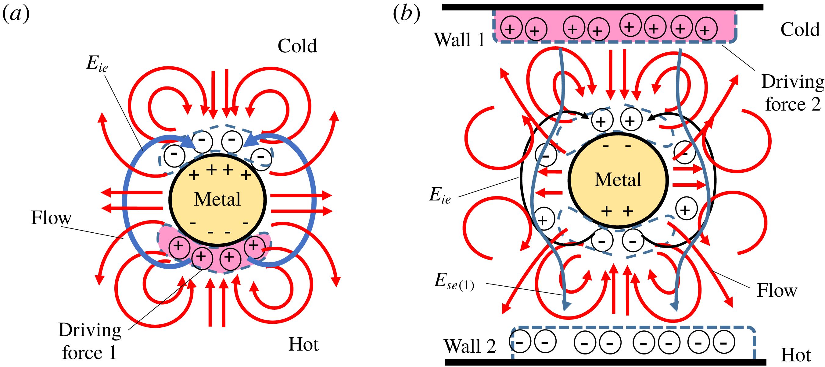
Figure 12 shows physical pictures of IE- and SE-NTKP. Namely, on the one hand, as shown in figure 12(a), IE-NTKP is driven by the excess positive ions that are pushed on the hotter side of the metal by the thermophoretic force. Namely, by the existence of the positive charge due to the excess charge on the hotter side of the metal, a negative charge is induced at the inside of the metal in the hotter region due to the image effect, whereas a positive charge is induced at the inside of the metal in the colder region because of the electrically neutral condition. Then, the positive charge at the inside of the metal attracts negative ions to the colder side of the metal. Consequently, two kinds of electric double layer are formed at the hotter and colder sides of the metal. Then, an electric field (
 $E_{ie}$
) from the positive charge at the hotter side to the negative charge at the colder side is generated and produces a quadrupolar vortex flow similar to ICEO, as shown in figure 12(a).
On the other hand, as shown in figure 12(b), SE-NTKP is driven by the excess positive ions that are pushed to the colder wall by the thermophoretic force. Namely, by the existence of the positive charge due to the excess charge at the colder wall, an electric field (
 $E_{se(2)}$
) in the hotter direction is generated and this induces positive and negative charges at the inside of the metal in the hotter and colder regions. Then, similar to the ordinary ICEO, the positive and negative ions attract counter-ions and form two kinds of electric double layer at the hotter and colder regions. However, different from the ordinary ICEO, the excess positive and negative ions that exist intrinsically near the hotter and colder sides due to the thermophoretic force weakens the zeta potential due to
 $E_{se(1)}$
around the metal. Further, at the same time, the latent excess ions generate an electric field (
 $E_{se(2)}=0.5E_{ie}$
) and suppress the tangential electric field outside of the double layer to the level of
 $E_{se(1)}-E_{se(2)}$
. The intrinsic positive ions are pushed out to the left and right sides in the hotter region, whereas the intrinsic negative ions are pushed out to the left and right sides in the colder region, as partially shown in figure 9(d). Consequently, an 8-pole vortex flow is generated for Modes 5 and 6, as shown in figure 12(b). Note that we observe an ordinary quadrupolar vortex flow for Mode 4 because of the difference in the early states which results in a difference in the memory effect, as will be discussed later.
4.7 AVF at the early stage
A weak AVF is generated at the early stage for Mode 1 as shown in figure 2(a), whereas an AVF is not generated for Mode 3, as shown in figure 3(a). This is because in Mode 1, positive and negative space charges are generated at
 $x\sim 0.3$
and 0.7, respectively, by the concentration polarization due to the charging current at the electric double layer of the metal. Similarly, by the thermophoretic flow near the wall, excess negative and positive space charges are generated at
 $x\sim 0.1$
and 0.9, respectively and thus an electric field in the
 $-x$
direction is generated. Consequently, an AVF is generated at the early stage. Further, the motion of the excess positive ions that forms a positive charge at the colder region are accelerated by the thermokinetic force, whereas the motion of the excess negative ions that forms a negative charge at the hotter region is suppressed by the thermokinetic force. Thus, the AVF at the colder region is stronger than for the hotter region. However, in Mode 3, a strong electric field in the
 $-x$
direction is generated, as shown in figure 10(d), because of the large temperature gradient near the wall at the early stage (in figure 3
f), whereas a space charge cannot be generated around the particle because of the low temperature gradient near the particle at the early stage (in figure 3
f). Thus, an AVF is not generated in Mode 3. Further, similar to the discussion of Mode 3, an AVF is not generated in Mode 6 because of the lack of a space charge region around the particle, as shown in figure 4(a).
4.8 Response time and the strong peak in Modes 2 and 3
Similar to the charging time of the electric double layer, we can define the characteristic time for the thermokinetic motion of the positive and negative ions as
 $$\begin{eqnarray}\displaystyle t_{\pm }=\frac{\unicode[STIX]{x1D706}_{D}^{2}}{2D_{\pm }\unicode[STIX]{x1D6FC}_{\pm }}. & & \displaystyle\end{eqnarray}$$
That is,
 $t_{+}/T_{0}\simeq 0.8\times 10^{-5}$
and
 $t_{+}/T_{0}\simeq 1.0\times 10^{-4}$
for the HCl solution. Here,
 $t_{+}$
corresponds to the peak time of
 $u_{max}$
for Modes 2 and 3 in figures 3(d) and 8(a) and this is the time during which H
 $^{+}$
ions move a distance of
 $\unicode[STIX]{x1D706}_{D}$
. Namely, since Cl
 $^{-}$
almost cannot move during
 $t_{+}$
, the strong electric field
 $E_{cp}$
in the
 $-x$
direction (in figure 10
d) occurs due to the concentration polarization owing to the strong flow of H
 $^{+}$
ions near the walls resulting from a large temperature gradient in the early stage, whereas there is no space charge around the metal. Thus, we consider that
 $E_{cp}$
produces a strong vortex flow of
 $f=0.76$
based on the ordinary ICEO mechanism at
 $t\simeq t_{+}\simeq 10^{-5}T_{0}$
in Modes 2 and 3 in figures 3(d) and 8(a) and it decays as
 $E_{cp}$
becomes small because of the passing boundary condition. Further, Cl
 $^{-}$
ions move a distance of
 $\unicode[STIX]{x1D706}_{D}$
during
 $t_{-}$
and thus the relaxation process is completed for Mode 1 at
 $t\simeq t_{-}\simeq 0.001T_{0}$
.
Mechanism of the memory effect. (a) Dependence of
 $\unicode[STIX]{x1D70C}$
on
 $y$
at
 $x=0.58$
and
 $t/T_{0}=2.0\times 10^{-4}$
. (b) Dependence of
 $\unicode[STIX]{x1D70C}$
on
 $y$
at
 $x=0.70$
and
 $t/T_{0}=2.0\times 10^{-4}$
. (c) AVF in Mode 4 at
 $t/T_{0}=2.0\times 10^{-4}$
(
 $f^{\prime }=15$
). (d) SVF (8-pole vortex flow) in Mode 5 at
 $t/T_{0}=2.0\times 10^{-4}$
(
 $f^{\prime }=15$
).

4.9 Mechanism of the memory effect
In figure 8(c),
 $u^{max}$
of Mode 4 has a small peak at
 $t/T_{0}=10^{-4}$
, whereas
 $u^{max}$
of Mode 5 continues to grow and it reaches a quasi-steady state at
 $t/T_{0}\simeq t_{-}\simeq 10^{-3}$
. We consider that this branching is the origin of the memory effect. Namely, similar to the discussion in §§ 4.7 and 4.8, more positive ions are transported to the hotter side of the metal cylinder in Mode 4 than Mode 5 at the early stage (
 $t/T_{0}=2\times 10^{-4}$
), as shown in figure 13(a). At the same time, the current causes negative charge regions around
 $(x,y)\simeq (0.7,0.6)$
and
 $(0.7,0.9)$
owing to the concentration polarization in Mode 4, as shown in figure 13(b). Thus, in Mode 4, the positive charge around
 $(x,y)\simeq (0.7,0.75)$
moves to the
 $x$
direction and the negative charge around
 $(x,y)\simeq (0.7,0.6)$
and
 $(0.7,0.9)$
moves to the metal. Consequently, an AVF is observed at
 $t/T_{0}=2\times 10^{-4}$
for Mode 4 in figure 13(c). In this mode, the positive charge is transported to negative charge region, whereas the negative charge is transported to the positive region. Thus, the maximum positive charge at
 $x>0.5$
decreases rapidly in Mode 4, as shown in figure 9(b) and the AVF changes to a SVF as the sign of the charge density around
 $(x,y)\simeq (0.6,0.75)$
changes from a positive to a negative value.
Further, in Mode 5, since the positive charge around
 $(x,y)\simeq (0.7,0.55)$
and
 $(0.7,0.95)$
is much larger than the positive charge around
 $(x,y)\simeq (0.7,0.75)$
, an SVF of the 8-pole type is observed at
 $t/T_{0}=2\times 10^{-4}$
, as shown in figure 13(d). In this mode, the positive charge is transported to the positive charge region. Thus, the maximum positive charge
 $\unicode[STIX]{x1D70C}^{max}$
at
 $x>0.5$
does not decrease rapidly in Mode 5, as shown in figure 9(b). We consider that the difference in the preserved maximum positive charge density at
 $x>0.5$
(the preserved maximum negative charge density at
 $x<0.5$
) in the laminate vortex flow at low Reynolds number is the main reason for the memory effect of NTKP. In addition, we consider that once the excess positive charge is pressed on the metal in the early stage (as shown in figure 13
a), the effect remains under the specific flows of Modes 4 and 5 because of the electrostatic attraction force between the image charge and the excess ions, even if the other induced charge is generated by the Seebeck effect; i.e. we consider that the electrostatic attraction force due to the image effect is the other main reason for the memory effect of NTKP.
4.10 Summary of the 1-D thermokinetic theory near the wall
By the discussion of §§ 4.1 and 4.2, with the Poisson equation we can write
 $$\begin{eqnarray}\displaystyle \unicode[STIX]{x1D70C}=\unicode[STIX]{x1D70C}_{wall}\text{e}^{-X/\unicode[STIX]{x1D706}_{D}}=-\unicode[STIX]{x1D700}\frac{\text{d}^{2}\unicode[STIX]{x1D6F7}}{\text{d}X^{2}} & & \displaystyle\end{eqnarray}$$
near the wall for the 1-D thermokinetic problem under the blocking boundary condition. Thus, by integrating (4.30) from
 $X=X$
to
 $X=\infty$
under the condition that
 $(-\unicode[STIX]{x1D700}(\text{d}\unicode[STIX]{x1D6F7}/\text{d}X))_{X=\infty }=Se(\unicode[STIX]{x1D735}T)_{0}$
, we obtain the electric field near the wall as
 $$\begin{eqnarray}\displaystyle E(X)~\left(=-\frac{\text{d}\unicode[STIX]{x1D6F7}}{\text{d}X}\right)=Se(\unicode[STIX]{x1D735}T)_{0}-\frac{\unicode[STIX]{x1D70C}_{wall}\unicode[STIX]{x1D706}_{D}}{\unicode[STIX]{x1D700}}\text{e}^{-X/\unicode[STIX]{x1D706}_{D}}. & & \displaystyle\end{eqnarray}$$
Here,
 $Se$
is a Seebeck coefficient in a general sense. Therefore, by using
 $\unicode[STIX]{x1D70E}=\unicode[STIX]{x1D70C}_{wall}\unicode[STIX]{x1D706}_{D}=\unicode[STIX]{x1D700}Se(\unicode[STIX]{x1D735}t)_{0}$
, we obtain
 $$\begin{eqnarray}\displaystyle E(0)=Se(\unicode[STIX]{x1D735}T)_{0}-\frac{\unicode[STIX]{x1D70C}_{wall}\unicode[STIX]{x1D706}_{D}}{\unicode[STIX]{x1D700}}=0. & & \displaystyle\end{eqnarray}$$
That is, we can understand that the ion blocking boundary condition corresponds to the zero-electric-field condition, which is often used in this field; see Majee & Würger (Reference Majee and Würger2012), Chikina et al. (Reference Chikina, Shikin and Varlamov2012, Reference Chikina, Shikin and Varlamov2015). In fact, we find that
 $(\unicode[STIX]{x2202}\unicode[STIX]{x1D719}/\unicode[STIX]{x2202}x)=0$
at
 $x=0$
and 1 at
 $t/T_{0}=0.004$
in figure 11(d).
Further, by the discussion of §§ 4.1 and 4.2, we can write
 $$\begin{eqnarray}\displaystyle & \displaystyle C_{+}\simeq C_{+0}\text{e}^{-X/l_{a}}+C_{0}, & \displaystyle\end{eqnarray}$$
 $$\begin{eqnarray}\displaystyle & \displaystyle C_{-}\simeq C_{+}-\frac{\unicode[STIX]{x1D70C}}{ez}\simeq C_{+}-\frac{\unicode[STIX]{x1D70C}_{0}}{ez}\text{e}^{-X/\unicode[STIX]{x1D706}_{D}}, & \displaystyle\end{eqnarray}$$
 $$\begin{eqnarray}\displaystyle & \displaystyle \frac{\text{d}C_{+}}{\text{d}X}\simeq -\frac{C_{+0}}{l_{a}}\text{e}^{-X/l_{a}}\simeq -2\unicode[STIX]{x1D6FC}_{+}(\unicode[STIX]{x1D735}T)_{0}C_{0}, & \displaystyle\end{eqnarray}$$
where
 $l_{a}$
is an apparent thermal characteristic length and
 $C_{+0}=C_{+}-C_{0}$
at
 $X=0$
. Although we obtain
 $$\begin{eqnarray}\displaystyle l_{a}\simeq \frac{C_{+0}}{2\unicode[STIX]{x1D6FC}_{+}(\unicode[STIX]{x1D735}T)_{0}}, & & \displaystyle\end{eqnarray}$$
 $l_{a}$
is not a universal value. Instead, it is defined as the distance, at which
 $\unicode[STIX]{x1D735}C_{+}=\unicode[STIX]{x1D735}C_{-}=0$
and thus
 $E(X)=\text{const}.$
Namely, since
 $\text{e}^{-4}\simeq 0.02$
, we can estimate
 $$\begin{eqnarray}\displaystyle l_{a}\sim 4\unicode[STIX]{x1D706}_{D}. & & \displaystyle\end{eqnarray}$$
In other words, although the universal characteristic length of the system is
 $\unicode[STIX]{x1D706}_{D}$
, an apparent characteristic length exists. In fact,
 $(C_{+}-C_{0})/C_{0}$
decays to
 $1/e$
times of
 $C_{+0}$
at
 $X\sim 0.08W=4\unicode[STIX]{x1D706}_{D}=4~\unicode[STIX]{x03BC}\text{m}$
in figure 11(a).
NTKP for a dielectric particle. (a) Dielectric-passing type NTKP (DP-NTKP). (b) Dielectric-blocking type NTKP (DB-NTKP).

4.11 The effect of conductance of the particle on NTKP
Interestingly, even when the particle (or cylinder) is made of a dielectric material, we can predict that a similar kind of vortex flow is generated under the existence of the large temperature gradient, as shown in figure 14. That is, a dielectric-passing type NTKP (DP-NTKP) and dielectric-blocking type NTKP (DB-NTKP) exist for the dielectric particle. Similar to IE-NTKP, the swifter positive ions are pressed onto the hotter side of the particle under the passing ion boundary condition and thus the concentration of the positive ion increases at the hotter side due to the thermophoretic force, whereas the concentration of the negative ion decreases at the colder side of the particle. Thus, a vortex flow similar to IE-NTKP is generated for DP-NTKP, as shown in figure 14(a). However, different from metal particles, we cannot expect the focusing effect of temperature described by (4.6) and the image effect of the metal. Thus, the zeta potential of the dielectric particle
 $\unicode[STIX]{x1D701}_{ie.d}^{\prime \prime }$
and the driving electric field of the dielectric particle
 $E_{ie.d}$
become
 $1/8$
times those of the metal; i.e.
 $\unicode[STIX]{x1D701}_{ie.d}^{\prime \prime }=(1/8)\unicode[STIX]{x1D701}_{ie}^{\prime \prime }$
and the driving electric field of the dielectric particle
 $E_{ie.d}=(1/8)E_{ie}$
. Therefore, the maximum flow velocity
 $u_{passing}^{dielectric}\simeq (1/64)u_{ie}$
. That is, we obtain the observable maximum flow velocity around the dielectric particle for the passing ion boundary condition as
 $$\begin{eqnarray}\displaystyle & \displaystyle u_{dp}\simeq \frac{\unicode[STIX]{x1D700}\unicode[STIX]{x1D701}_{ie.d}^{\prime \prime }}{2\unicode[STIX]{x1D707}}E_{ie.d}, & \displaystyle\end{eqnarray}$$
 $$\begin{eqnarray}\displaystyle & \displaystyle \unicode[STIX]{x1D701}_{ie.d}^{\prime \prime }\simeq \sqrt{2}\unicode[STIX]{x1D6FC}_{+}(\unicode[STIX]{x1D735}_{n}\tilde{T})_{0}\frac{\unicode[STIX]{x1D706}_{D}^{3}\unicode[STIX]{x1D70C}_{c}}{\unicode[STIX]{x1D700}W}, & \displaystyle\end{eqnarray}$$
 $$\begin{eqnarray}\displaystyle & \displaystyle E_{ie.d}\simeq -\frac{4\unicode[STIX]{x1D6FC}_{+}(\unicode[STIX]{x1D735}_{n}\tilde{T})_{0}{\displaystyle \frac{\unicode[STIX]{x1D706}_{D}^{3}\unicode[STIX]{x1D70C}_{c}}{\unicode[STIX]{x1D700}W}}}{\unicode[STIX]{x03C0}(a+\unicode[STIX]{x1D706}_{D})}. & \displaystyle\end{eqnarray}$$
Further, similar to SE-NTKP, the swifter positive ions are pressed onto the colder side of the wall under the blocking ion boundary condition and thus the concentration of the positive ion increases at the colder wall due to the thermophoretic force, whereas the concentration of the negative ion decreases at the hotter wall. However, different from metal particles, the excess swifter positive ions still exists on the hotter side of the particle and the shortage of the swifter positive ions exists at the colder side, since the image (or induced charge) effect of a dielectric particle is almost negligible compared to that of metal. Thus, the positive and negative charges on the hotter and colder sides of the particle move by the Seebeck electric field due to the charge near the wall. Therefore, a quadrupolar but asymmetrical vortex flow is generated around the dielectric particle for DB-NTKP under the blocking boundary condition, as shown in figure 14(b). Further, similar to the discussion of (4.11) and (4.5), we obtain the observable maximum flow velocity around the dielectric particle for the blocking ion boundary condition as
 $$\begin{eqnarray}\displaystyle & \displaystyle u_{db}\simeq \frac{\unicode[STIX]{x1D700}\unicode[STIX]{x1D701}_{db}^{\prime \prime }}{2\unicode[STIX]{x1D707}}E_{db}, & \displaystyle\end{eqnarray}$$
 $$\begin{eqnarray}\displaystyle & \displaystyle \unicode[STIX]{x1D701}_{db}^{\prime \prime }\simeq \sqrt{2}\unicode[STIX]{x1D6FC}_{+}(\unicode[STIX]{x1D735}_{n}\tilde{T})_{0}\frac{\unicode[STIX]{x1D706}_{D}^{3}\unicode[STIX]{x1D70C}_{c}}{\unicode[STIX]{x1D700}W}, & \displaystyle\end{eqnarray}$$
 $$\begin{eqnarray}\displaystyle & \displaystyle E_{db}\simeq 2E_{se(1)}\sin \frac{\unicode[STIX]{x03C0}}{4}\simeq 2\sqrt{2}\unicode[STIX]{x1D6FC}_{+}(\unicode[STIX]{x1D735}_{n}\tilde{T})_{0}\frac{\unicode[STIX]{x1D706}_{D}^{2}\unicode[STIX]{x1D70C}_{c}}{\unicode[STIX]{x1D700}W}, & \displaystyle\end{eqnarray}$$
where we assume that the effect of
 $E_{ie.d}$
is negligible for the dielectric particle.
Note that we consider that the charge on the hotter side is negligible in DP- and DB-NTKP because of the continuous instant supply of positive ions from the hotter region and thus the vortex flow at the colder side is negligible, as expressed by the broken lines in figure 13. Further, by using (4.38)–(4.43), we obtain
 $E_{db}\simeq 350~\text{V}~\text{m}^{-1}$
,
 $\unicode[STIX]{x1D701}_{db}^{\prime \prime }\simeq 0.17$
mV and
 $u_{db}\simeq 0.021~\unicode[STIX]{x03BC}\text{m}~\text{s}^{-1}$
in DB-NTKP;
 $E_{dp}\simeq 26~\text{V}~\text{m}^{-1}$
,
 $\unicode[STIX]{x1D701}_{dp}^{\prime \prime }\simeq 0.17$
mV and
 $u_{dp}\simeq 0.0016~\unicode[STIX]{x03BC}\text{m}~\text{s}^{-1}$
in DP-NTKP. Thus, there is a possibility of observing DB-NTKP, although DP-NTKP might be difficult to observe.
Relevant experiments on NTKP.

4.12 Relevant experiments
Discussion of DB-NTKP provides a simple theory for the thermophoresis (or Soret effect) of the electrically neutral dielectric particle, although a thermophoretic theory for charged colloids was provided by Würger (Reference Würger2008). Namely, the thermophoretic velocity
 $U$
of the dielectric particle is provided as
 $$\begin{eqnarray}\displaystyle U_{th.d}\sim u_{db}\sim \frac{\unicode[STIX]{x1D700}\unicode[STIX]{x1D706}_{D}}{2\unicode[STIX]{x1D707}}[2\unicode[STIX]{x1D6FC}_{+}(\unicode[STIX]{x1D735}_{n}\tilde{T})_{0}]^{2}\left(\frac{\unicode[STIX]{x1D706}_{D}^{2}\unicode[STIX]{x1D70C}_{c}}{\unicode[STIX]{x1D700}W}\right)^{2}\sim \frac{\unicode[STIX]{x1D700}\unicode[STIX]{x1D706}_{D}}{2\unicode[STIX]{x1D707}}[Se(\unicode[STIX]{x1D735}T)_{0}]^{2}, & & \displaystyle\end{eqnarray}$$
where
 $(\unicode[STIX]{x1D706}_{D}^{2}\unicode[STIX]{x1D70C}_{c}/\unicode[STIX]{x1D700}W)=(1/2)\unicode[STIX]{x1D6F7}_{c}\simeq 12.9$
mV. The surprising aspect of (4.44) is that the Soret effect due to an ion that is thermokinetically pressed onto the particle is considered to be a kind of NTKP since
 $u_{th.d}\propto (\unicode[STIX]{x1D735}T)_{0}^{2}$
; thus,
 $D_{T}$
and
 $S_{T}$
are proportional to
 $\unicode[STIX]{x1D735}T$
. In addition, our theory predicts that a dielectric particle moves toward the colder region when the thermokinetically swifter ion is a positive ion (e.g. H
 $^{+}$
) in the electrolyte, as shown in figure 14(b), whereas a dielectric particle moves toward the hotter region when the thermokinetically swifter ion is a negative ion (e.g. OH
 $^{-}$
) in the electrolyte as shown in figure 15(a); this prediction agrees with the experimental results of Vigolo, Buzzaccaro & Piazza (Reference Vigolo, Buzzaccaro and Piazza2010). Further, our theory predicts that
 $u_{th.d}$
decreases as
 $C_{0}$
increases through
 $\unicode[STIX]{x1D706}_{D}$
and this prediction also agrees with the experimental results of Vigolo et al. (Reference Vigolo, Buzzaccaro and Piazza2010).
We consider that the self-propelled motion of the Janus particle irradiated by the laser (Jiang et al.
Reference Jiang, Yoshinaga and Sano2010) can be explained by NTKP theory, since the experimental thermokinetic velocity of the self-propelled Janus particle
 $u_{J}$
(Jiang et al.
Reference Jiang, Yoshinaga and Sano2010) is not proportional to
 $\unicode[STIX]{x1D735}T$
globally in the sense that the line of the dependence (
 $u_{J}$
versus
 $\unicode[STIX]{x1D735}T$
) does not go through the zero point, as mentioned before. Namely, since
 $\unicode[STIX]{x1D6FC}_{+}^{H^{+}}=2.7$
and
 $\unicode[STIX]{x1D6FC}_{-}^{OH^{-}}=3.4$
in water, the swifter negative ions are pressed onto the colder dielectric surface, whereas the slower positive ions remain on the colder dielectric surface, as illustrated in figure 15(b). Then, a negative induced charge is generated on the metal surface, whereas a positive induced charge is generated at the interface between the metal and the dielectric material and this attracts negative ions toward the metal region. Consequently, the strong surface flow toward the metal region occurs on the dielectric surface. Thus, the Janus particle moves toward the dielectric end in water. Further, by a similar mechanism, the Janus particle moves toward the metal end in a Triton X-solution because of the decrease in the pH due to the effect of the hydroxy group of the Triton X-solution. This explanation agrees with the experimental results (Jiang et al.
Reference Jiang, Yoshinaga and Sano2010) and thus our theory is justified to some extent.
4.13 Three-dimensional model and the general picture of NTKP
Through the discussion of the previous sections, we recognized that NTKP is a general phenomenon that can be found in both metal and dielectric particles. That is, the original driving force of NTKP is the excess ions pressed onto the particle by the thermokinetic force due to the thermal gradient and the flow around the particle is generated by the interaction between the excess ions and the electric field that is made by the excess ions themselves and/or the Seebeck electric fields due to the blocking boundary condition on the wall of the liquid chamber; thus, the flow velocity is intrinsically proportional to the square of the temperature gradient. The difference between the metal NTKP and the dielectric NTKP is the strength of the polarization of the particle resulting from the permittivity
 $\unicode[STIX]{x1D700}$
and the strength of the local temperature gradient of the particle resulting from the thermal conductivity
 $\unicode[STIX]{x1D706}$
. Namely, by the difference of
 $\unicode[STIX]{x1D700}$
and
 $\unicode[STIX]{x1D706}$
, the flow velocity of the metal NTKP is approximately eight times of that of the dielectric NTKP.
Here, we consider a 3-D model using the Debye–Hükel approximation for the thick electric double layer (i.e.
 $\unicode[STIX]{x1D706}_{D}\gg a$
). That is, for the 3-D dielectric particle, we can approximate that
 $(\unicode[STIX]{x03C0}a^{2}\unicode[STIX]{x1D700}Se\unicode[STIX]{x1D735}T)E_{interact}\simeq 6\unicode[STIX]{x1D707}Ua$
for the blocking boundary condition, where
 $q\simeq \unicode[STIX]{x1D700}Se\unicode[STIX]{x1D735}T$
is the charge of the swifter excess ions on the hotter side,
 $U$
is the velocity of the particle and
 $E_{interact}$
is an electric field that interacts with the charge around the particle; i.e. we obtain that
 $$\begin{eqnarray}\displaystyle U_{dielectric}^{\unicode[STIX]{x1D706}_{D}\gg a}\sim \frac{\unicode[STIX]{x1D700}a}{6\unicode[STIX]{x1D707}}(Se\unicode[STIX]{x1D735}T)E_{interact}. & & \displaystyle\end{eqnarray}$$
Further, by multiplying
 $(3/2)$
and (4.45), we obtain
 $U$
for the thin electric double layer (i.e.
 $\unicode[STIX]{x1D706}_{D}\ll a$
); i.e.
 $$\begin{eqnarray}\displaystyle U_{dielectric}^{\unicode[STIX]{x1D706}_{D}\ll a}\sim \frac{\unicode[STIX]{x1D700}a}{4\unicode[STIX]{x1D707}}(Se\unicode[STIX]{x1D735}T)E_{interact}. & & \displaystyle\end{eqnarray}$$
Although
 $U$
generally depends on the difference between the velocities of the vortex flows on the hotter and colder sides of the particle,
 $u^{max}$
is generally described as
 $$\begin{eqnarray}\displaystyle u_{general}^{max}\sim f_{p}f_{\unicode[STIX]{x1D705}}\frac{\unicode[STIX]{x1D700}a}{4\unicode[STIX]{x1D707}}(Se\unicode[STIX]{x1D735}T)E_{interact}, & & \displaystyle\end{eqnarray}$$
where
 $f_{p}$
is the factor due to
 $\unicode[STIX]{x1D700}$
and
 $\unicode[STIX]{x1D706}$
and
 $f_{\unicode[STIX]{x1D705}}$
is the factor due to
 $\unicode[STIX]{x1D705}=a/\unicode[STIX]{x1D706}_{D}$
. Note that
 $f_{p}\simeq 8$
for the metal and
 $f_{p}\simeq 1$
for the dielectric particle;
 $f_{\unicode[STIX]{x1D705}}\simeq 1$
at
 $\unicode[STIX]{x1D705}=\infty$
and
 $f_{\unicode[STIX]{x1D705}}\simeq (2/3)$
at
 $\unicode[STIX]{x1D705}=0$
;
 $E_{interact}\sim Se\unicode[STIX]{x1D735}T$
.
4.14 The influence of the electrolyte concentration on IE- and SE-NTKP
From (4.16) and (4.28), the maximum flow velocities of IE- and SE-NTKP depend on the concentration since
 $\unicode[STIX]{x1D706}_{D}\propto 1/\sqrt{C_{0}}$
and
 $\unicode[STIX]{x1D70C}_{c}=ezC_{0}$
. In detail,
 $u_{ie}\propto 1/C_{0}$
and thus
 $u_{ie}\rightarrow 0$
at
 $C_{0}\rightarrow \infty$
in IE-NTKP. Further,
 $u_{se}$
increases as
 $C_{0}$
increases in SE-NTKP. This is because
 $E_{se}$
increases as
 $C_{0}$
increases, since
 $E_{se(2)}\propto 1/\sqrt{C_{0}}$
and
 $E_{se(1)}$
is constant. In addition,
 $|\unicode[STIX]{x1D701}_{se}^{\prime \prime }|$
increases as
 $C_{0}$
increases, since
 $\unicode[STIX]{x1D70C}_{se.m(2)}(\unicode[STIX]{x1D706}_{D}^{2}/\unicode[STIX]{x1D700})\propto 1/\sqrt{C_{0}}$
and
 $\unicode[STIX]{x1D70C}_{se.m(1)}(\unicode[STIX]{x1D706}_{D}^{2}/\unicode[STIX]{x1D700})$
is constant. Thus, at
 $C_{0}\rightarrow \infty$
, we obtain
 $$\begin{eqnarray}\displaystyle u_{se}\rightarrow -\frac{\unicode[STIX]{x1D700}a}{\unicode[STIX]{x1D707}}[2\unicode[STIX]{x1D6FC}_{+}(\unicode[STIX]{x1D735}_{n}\tilde{T})_{0}]^{2}\left(\frac{\unicode[STIX]{x1D706}_{D}^{2}\unicode[STIX]{x1D70C}_{c}}{\unicode[STIX]{x1D700}W}\right)^{2}, & & \displaystyle\end{eqnarray}$$
which is consistent with (4.47). Namely, as a whole, our new theories of IE-, SE-, DP- and DB-NTKP are consistent with each other and they explain various numerical results under the various conditions reasonably well, as discussed in the previous sections. Thus, our new theories are useful. Nevertheless, we may need to develop a more precise theory in the future, since (4.47) suggests that
 $u_{ie}=\text{const}.$
for various
 $C_{0}$
. In addition, we may need to reconsider ‘
 $Se$
’ in relation to NTKP in the future since
 $E_{interact}$
may change continuously from zero to
 $S_{e}(\unicode[STIX]{x1D6FB}T)_{0}$
defined by (2.23) for the passing boundary condition; e.g.
 $E_{interact}$
on a vertical plate between the hotter and colder electrodes is probably small since there are no pressed excess ions on the wall, whereas
 $E_{interact}$
on a horizontal plate between the hotter and colder electrodes is provably near to the value of
 $S_{e}(\unicode[STIX]{x1D6FB}T)_{0}$
of (2.23).
4.15 Convection flow
We neglect convection flow for our calculation. This is because, at least theoretically, it is prevented when the hotter wall is placed at the higher place. Moreover, the Rayleigh number
 $Ra\equiv (g\unicode[STIX]{x1D6FD}\unicode[STIX]{x0394}TW^{3}/\unicode[STIX]{x1D708}a_{T})\simeq 2.29\times 10^{-14}\ll 1$
, Marangoni number
 $|Ma|\equiv ((\unicode[STIX]{x2202}\unicode[STIX]{x1D70E}/\unicode[STIX]{x2202}T)\unicode[STIX]{x0394}TW/\unicode[STIX]{x1D707}a_{T})\simeq 0.42\times 10^{-3}\ll 1$
and
 $Ra/|Ma|=(g(\unicode[STIX]{x2202}\unicode[STIX]{x1D70C}/\unicode[STIX]{x2202}T)W^{2}/(\unicode[STIX]{x2202}\unicode[STIX]{x1D70E}/\unicode[STIX]{x2202}T))\simeq 5.5\times 10^{-11}\ll 1$
, where
 $\unicode[STIX]{x1D70E}$
is the surface tension,
 $\unicode[STIX]{x1D707}=0.668~\text{m}^{2}~\text{s}^{-1}$
is the kinematic viscosity,
 $\unicode[STIX]{x1D6FD}=-(1/\unicode[STIX]{x1D70C})(\unicode[STIX]{x2202}\unicode[STIX]{x1D70C}/\unicode[STIX]{x2202}T)=0.38\times 10^{-3}$
is the coefficient of thermal expansion,
 $\unicode[STIX]{x0394}T=50~\text{K}$
,
 $W=50~\unicode[STIX]{x03BC}\text{m}$
,
 $\unicode[STIX]{x0394}\unicode[STIX]{x1D70E}=8.26~\text{mN}~\text{m}^{-1}$
,
 $\unicode[STIX]{x1D707}=0.653$
mPa s,
 $a_{T}=1.52~\text{m}^{2}~\text{s}^{-1}$
and
 $g=9.8~\text{m}~\text{s}^{-2}$
. Thus, in our system, Marangoni convection (due to the difference in surface tension) and Rayleigh convection (due to the difference in density) are suppressed because of the viscous force. In fact, convection flow is usually suppressed in experiments in this field (Agar Reference Agar, Delahay and Tobias1963; Bonetti et al.
Reference Bonetti, Nakamae, Roger and Guenoun2011). For example, Bonetti et al. (Reference Bonetti, Nakamae, Roger and Guenoun2011) prevented a convection flow and reported huge Seebeck coefficients in non-aqueous electrolytes by using a Teflon hollow cylinder (15 mm high) sealed by 5 mm thick sapphire window plates and setting the hotter sapphire plate (
 $T=28$
–
 $75\,^{\circ }\text{C}$
) at the higher position and the colder sapphire plate (
 $T=24\,^{\circ }\text{C}$
) at the lower position; i.e. experimentally a convection flow can be suppressed significantly under the condition of a temperature difference of 4–51 K over a gap distance of 15 mm. Thus, to neglect convection flow in our simulation is justified. Note that the vertically sandwiched configuration that places the hotter plate at the higher position is useful to minimize a natural convection flow since convection flow occurs by the upward motion of the lower density solution at the lower position. Further, sapphire plates of large thermal conductivity were used to establish a uniform heating of the sample cross-section and a stable temperature gradient.
4.16 The effect of the temperature dependence of
 $D_{\pm }$
and
$\unicode[STIX]{x1D707}$


In figure 5, the effect of the temperature dependence of
 $D_{\pm }$
and
 $\unicode[STIX]{x1D707}$
is rather small. This is because (2.3) already includes the main temperature dependence of the parameters even if we assume that
 $D_{\pm }$
and
 $\unicode[STIX]{x1D707}$
are constant. Further, the NTKP characteristic is mainly governed in the region of an electric double layer of thickness
 $\unicode[STIX]{x1D706}_{D}$
(
 $\simeq 1~\unicode[STIX]{x03BC}\text{m}$
) and the surface temperature of the metal cylinder is assumed to be constant; i.e. the dominant temperature difference is considered as
 $\unicode[STIX]{x0394}T^{dominant,ntkp}\simeq 2\unicode[STIX]{x1D706}_{D}(\unicode[STIX]{x1D735}T)_{0}=2~\text{K}$
and thus the effect of the temperature dependence of the parameters is small. Note that the dominant temperature difference for the ordinary linear thermokinetic phenomenon (LTKP) is usually considered as
 $\unicode[STIX]{x0394}T^{dominant,ltkp}\simeq 2a(\unicode[STIX]{x1D735}T)_{0}=10~\text{K}$
since the thermal conductivity of a non-polarizable particle is assumed to be compatible with that of the surrounding solution. Thus, the effect of the temperature dependence of the parameters of the NTKP is much smaller than that of the ordinary thermokinetic phenomena.
4.17 Physical meaning of the comparative study of the various modes
By comparing the numerical results for the passing and blocking boundary conditions, we first recognized the precise physical picture of NTKP. Thus, those boundary conditions are needed for our analysis. Specifically, only the blocking boundary condition (or only the zero-electric-field condition) is usually considered at the wall in the field of thermokinetics, although the researchers into thermogalvanic cells might be interested in the passing boundary condition. However, since SE-NTKP includes the effect of IE-NTKP, the blocking boundary condition is required to clarify IE-NTKP. Further, the passing and blocking boundary conditions are known as major boundary conditions to understand the phenomena in the field of electrokinetics. Thus, even in the field of the thermokinetic phenomena, we consider that the passing boundary condition will be important in the future.
Further, by comparing the numerical results for the different initial conditions on the temperature distribution, we find that the memory effect (or hysteresis effect of the temperature) exists in SE-NTKP. Specifically, we consider (2.1) as the limit of
 $a_{T}\rightarrow \infty$
for Modes 1 and 4 and the suddenly applied hot and cold temperatures at the walls for Modes 2 and 5. Here, the suddenly applied hot and cold temperatures are idealized conditions with instant heating and cooling of walls. However, at least instant heating can be realized to some extent experimentally by using a thin film heater in the water and thus a situation similar to Modes 2 and 5 will occur experimentally. Thus, the initial conditions for temperature are useful to understand non-steady phenomena, as a first step.
In addition, since we consider the temperature difference
 $\unicode[STIX]{x0394}T$
is 50 K across the chamber, the variation of the coefficients of viscosity, mobility and diffusion is not negligible as a general (but too strict) argument. However, consideration of the temperature dependences of these parameters complicates the intrinsic phenomena in NTKP. Thus, as a challenging study, we calculate both situations. Through these time-consuming calculations, we first succeed in clarifying NTKP and answering the general criticism, although the effect of the temperature dependence is reasonably small as a result, as discussed in § 4.16.
5 Conclusion
In conclusion, we clarified the general physical picture of NTKP. That is, by performing a non-steady multi-physics direct simulation, we have shown the following. (i) The maximum flow velocity around a metal is generally proportional to the square of the temperature gradient. (ii) NTKP is classified into two types according to its mechanism; i.e. IE-NTKP for the passing boundary condition and SE-NTKP for the blocking boundary condition. (iii) The memory effect appears in SE-NTKP via the difference in the temperature gradient at the early stage. (iv) The strong peak of
 $u^{max}$
appears at the early stage for the passing boundary condition. (v) The temperature dependence effect of the parameters is rather small, but detectable. (vi) Further, through the discussion, new theories on IE-NTKP and SE-NTKP are provided and they explain the numerical results in a self-consistent manner. (vii) AVF is explained by the concentration polarization due to the rapid transportation of the swifter ions in the early stage. (viii) Response time is explained by the thermokinetic diffusion time; i.e.
 $t_{\pm }=\unicode[STIX]{x1D706}_{D}^{2}/2D_{\pm }\unicode[STIX]{x1D6FC}_{\pm }$
. (ix) The memory effect in SE-NTKP (in particular Mode 5) is qualitatively explained by the attractive force due to the image effect and the preserving effect of the initial charge due to the 8-pole vortex flow. (x) A simple 1-D thermokinetic theory is provided and it shows that the blocking boundary condition leads to the zero-electric-field condition and
 $\unicode[STIX]{x1D706}_{D}$
is the only true characteristic length for our system, although an apparent thermal characteristic length (
 $l_{a}\sim 4\unicode[STIX]{x1D706}_{D}$
) exists. (xi) A theory of NTKP for the dielectric particle is provided and it seems to explain the Soret effect of a neutral dielectric particle to some extent. (xii) Self-propelled motion of the Janus particle irradiated by a laser is successfully explained as the framework of NTKP theory. (xiii) A simple 3-D model of NTKP is provided and it clarifies NTKP for the general particle. We believe that our findings give new insights into the better understanding of the general thermokinetic phenomena ranging from a metallic particle to a dielectric particle. In particular, the most surprising aspect of our findings is that there is the possibility that NTKP exists universally. Further, similar to ICEO, the 3-D NTKP effects of the 3-D particles or structures (e.g. the transportation effect due to the broken symmetry, the rotation effect of an ellipsoid particle, the connecting effect due to the hydrodynamic interaction between particles, etc.) will be explored with promising applications in the future.
Acknowledgement
This work was partially supported by JSPS KAKENHI Grant No. JP16K05650.