1 Introduction
The flow induced by the impulsive rotation of a sphere, immersed in a body of fluid, is an example of a very simple system that exhibits a wide range of fundamental and important fluid mechanical phenomena, each with a broad range of applicability to other spatially and temporally developing flows. One of the most important phenomena that arises in this flow is the collision in the boundary layer that develops on the sphere’s surface; the centrifugal force that arises due to the spinning sphere serves to advect the fluid in the boundary layer from the poles to the equator where a collision occurs. The study of this boundary-layer development process, and the subsequent collision, was first considered by Howarth (Reference Howarth1951) and subsequently by Banks (Reference Banks1965, Reference Banks1976) and Banks & Zaturska (Reference Banks and Zaturska1979). The latter study served to provide an explanation of the boundary-layer collision in the context of the development of a finite-time singularity in the boundary-layer equations. The structure of this singularity, and the time at which it occurs, have been the focus of numerous studies; for example Simpson & Stewartson (Reference Simpson and Stewartson1982), and later Dennis & Duck (Reference Dennis and Duck1988), were primarily focussed upon the singularity structure, whereas the work of van Dommelen (Reference van Dommelen1990) exploited the Lagrangian approach developed by Cowley, van Dommelen & Lam (Reference Cowley, van Dommelen and Lam1990), to obtain a more accurate prediction of the time of the onset of the finite-time singularity.
In addition to their relevance to impulsively started flows, boundary-layer collisions are also important in the context of unsteady boundary-layer separation, and also arise in a number of other simple, but important, fluid flow problems. One such example is found in the starting flow in a curved pipe; Riley (Reference Riley1998) demonstrated that the sudden imposition of a constant pressure gradient results in a collision of boundary layers at the inside bend of the pipe, the collision being another manifestation of a finite-time singularity in the boundary-layer equations. Another physical manifestation of this type of boundary-layer breakdown occurs in the entry flow in a curved duct. Stewartson, Cebeci & Chang (Reference Stewartson, Cebeci and Chang1980) demonstrated that the breakdown gives rise to a thickening of the boundary layer on the duct wall. Experimental evidence for this collision process, and the subsequent thickening of the boundary layer, has been provided by Kluwick & Wohlfahrt (Reference Kluwick and Wohlfahrt1986) (for the entry flow in a curved duct) and Boirin, Deplano & Pelissier (Reference Boirin, Deplano and Pelissier2007) (for the starting flow in curved duct).
Our concern here is not with internal flows but the flow due to a rigid sphere, suddenly imparted with angular momentum. This much studied flow has been used as the paradigm for the exploration of both the development of finite-time singularities in the boundary-layer equations, and the consequential unsteady boundary-layer separation that results from the singularity. Unfortunately, the flow dynamics after the development of this singularity is not (yet) amenable to asymptotic analysis (at high Reynolds numbers), and no suitable asymptotic description is possible at lower Reynolds numbers. To further elucidate the behaviour of this flow, one must therefore resort to either experimental means or computational methods, or both.
The first experiments on the flow due to a rotating sphere were undertaken in the early 1960s by Bowden and colleagues (Bowden & Lord Reference Bowden and Lord1963; Bowden & Harbour Reference Bowden and Harbour1966), in which a metal sphere was magnetically levitated and spun using induction. The induction served to heat the surface of the sphere, which, in turn, modified the density of the fluid (air, and other more exotic gases) within the boundary layer at the sphere’s surface. The result was a radial jet ejected from the sphere’s surface with a slightly different density from that of the surrounding quiescent fluid. This density difference allowed Bowden & Lord (Reference Bowden and Lord1963) to make use of schlieren photography to visualise the radial jets. Later experiments by Calabretto et al. (Reference Calabretto, Levy, Denier and Mattner2015a ) used simple dye-flow visualisation techniques to render the radial jet visible.
Those first experiments by Bowden & Lord (Reference Bowden and Lord1963) did not report the ambient temperature of the air in the experiment, thus making comparison with more recent results (and the results to be presented here) somewhat difficult. Assuming that Bowden & Lord’s working medium was air, that the experiments were conducted at atmospheric pressure and that the ambient temperature in the laboratory was
 $20\,^{\circ }\text{C}$
, then a reasonable estimate for the fluid’s kinematic viscosity is
 $\unicode[STIX]{x1D708}=15~\text{mm}^{2}~\text{s}^{-1}$
(Batchelor Reference Batchelor1967). Bowden & Lord (Reference Bowden and Lord1963) used a metal sphere of
 $\frac{1}{2}$
in. diameter (radius
 $a=0.00635$
m) and reported experiments with angular velocities
 $\unicode[STIX]{x1D6FA}$
in the range
 $6~\text{m s}^{-1}$
to
 $18~\text{m s}^{-1}$
. With the Reynolds number defined, in Bowden & Lord (Reference Bowden and Lord1963), as
 $$\begin{eqnarray}Re=\frac{a^{2}\unicode[STIX]{x1D6FA}}{\unicode[STIX]{x1D708}},\end{eqnarray}$$
their experiments covered Reynolds numbers from
 $Re\approx 2500$
to
 $Re\approx 7500$
, respectively. This range of Reynolds numbers puts their experiments below the theoretical predictions, derived from a linear stability analysis, of Garret & Peake (Reference Garret and Peake2002) who found a critical Reynolds number of around
 $Re=11\,000$
. It is worth noting that Bowden & Lord (Reference Bowden and Lord1963) comment that the flow in their work may be assumed to be laminar. They base this upon the fact that, at the time their experiments were conducted, the critical value of the Reynolds number for transition to turbulence on a disk was approximately
 $3\times 10^{5}$
, and that the highest Reynolds numbers in their experiments were below this critical value. Nevertheless, no mention is made in Bowden & Lord (Reference Bowden and Lord1963) of any instabilities being observed.
Since those early experiments of Bowden, there have been a number of other experimental studies of the rotating sphere, with a particular emphasis on the transition to turbulence within the boundary layer on the surface of the sphere. Most important amongst these are those conducted by Kohama & Kobayashi (Reference Kohama and Kobayashi1983) who clearly demonstrate that an instability develops within the boundary layer at a latitude of approximately
 $70^{\circ }$
from the pole at Reynolds numbers above approximately
 $Re=11\,000$
.
Later experimental work of Hada & Ito (Reference Hada and Ito2003) demonstrated that the radial jet that arises from the boundary-layer collision, develops an absolute instability at a Reynolds number of
 $2600$
(we have converted Hada & Ito’s (Reference Hada and Ito2003) rotation rates, using a value for the kinematic viscosity, of air at
 $20\,^{\circ }\text{C}$
, of
 $\unicode[STIX]{x1D708}=15~\text{mm}^{2}~\text{s}^{-1}$
, a radius of
 $50$
mm, a value of
 $\unicode[STIX]{x1D6FA}=147~\text{rev}~\text{min}^{-1}=2\unicode[STIX]{x03C0}\times 147/60~\text{rad}~\text{s}^{-1}$
, to give a Reynolds number defined by (1.1) of
 $2600$
), which is an order of magnitude lower than the critical Reynolds number for the boundary layer reported by Kohama & Kobayashi (Reference Kohama and Kobayashi1983). There is no evidence of this instability in the Bowden & Lord experiments at such a low Reynolds number (see their figure 2
a), although at higher
 $Re$
there is a clear shortening of the radial jet. This suggests that the low critical Reynolds number found by Hada & Ito (Reference Hada and Ito2003) may be due to an asymmetry introduced through their experimental set-up.
We note that the computational results of Calabretto et al. (Reference Calabretto, Levy, Denier and Mattner2015a ) demonstrate the natural development of an absolute instability in the radial jet. By natural, we mean in the sense that the computational scheme is not forced through, or by, the imposition of any external disturbance. The absolute instability of the radial jet, observed in Calabretto et al. (Reference Calabretto, Levy, Denier and Mattner2015a ), develops at a much higher Reynolds number than that seen in the experiments of Hada & Ito (Reference Hada and Ito2003).
Here we will focus on two fundamental aspects of this problem, namely the boundary-layer collision, and the jet development and its subsequent instability. To date, there have been two competing theories put forward for the high-Reynolds-number structure of the (steady) post-collisional flow near the equator. The first, by Stewartson (Reference Stewartson and Görtler1958), posits a dual layer structure, consisting of an outer, inviscid, ‘corner’ region at the equator/sphere junction. This outer
 $O(Re^{-1/2})\times O(Re^{-1/2})$
-thick layer is supplemented by a largely passive inner viscous layer. Without solving the equations in this region, Stewartson provides a heuristic argument for the existence of small region of reversed flow near the sphere’s equator. The second theory, put forward by Smith & Duck (Reference Smith and Duck1977), predicts a large-scale recirculation region, symmetric with respect to the equator. This description requires an
 $O(Re^{-3/14})\times O(Re^{-3/14})$
-thick distinguished asymptotic structure. We will explore this post-collision structure through a combination of experiment and high resolution direct numerical simulation of the flow, at never before achieved Reynolds numbers. We will also explore the mechanism behind the jet instability, demonstrating one possible receptivity mechanism that can arise if any small asymmetry exists in the experimental apparatus.
The structure of the paper is then as follows: after providing a description of the experimental set-up in § 2, we present the results of a new series of experiments that demonstrate the boundary-layer collision, radial jet development and subsequent absolute instability. These are prefaced by some computational results, for moderate Reynolds numbers, that help provide some context for our experimental results. This is followed in § 4 with new computational results, on flows up to
 $Re=O(10^{5})$
, allowing us to shed further light on the steady, post-singularity structure of the global flow at very high Reynolds numbers. We close in § 5 with a summary of our findings and some thoughts on possible future work.
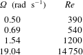
Experimentally measured rotation rates and corresponding Reynolds numbers.

2 Experimental set-up
A solid sphere (in our case an ‘
 $8$
-ball’) of diameter
 $57.15\pm 0.127$
mm (these tolerances are as quoted by the manufacturer, and were verified using digital callipers), was mounted on a
 $4$
mm metal rod. This was achieved by drilling a hole through the (approximate) centre of the sphere, then gluing the rod into the hole. With the rod mounted through the sphere, the tolerance of this sphere/rod system was determined optically and found to be accurate to within
 $0.1$
mm. The rod was placed in a Perspex tank, with a depth and width of
 $600$
mm and height of
 $300$
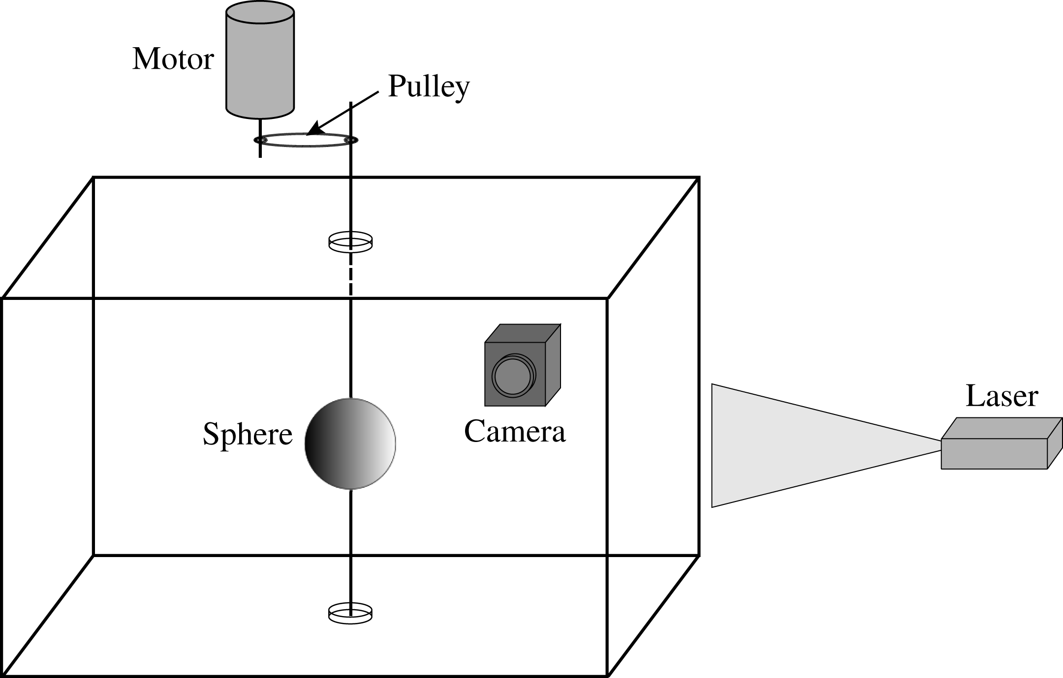
mm, and held in place at the top and bottom of the tank with small, circular Perspex brackets. The rod length was chosen so that it extended out through a hole in the tank lid, allowing for a variable speed DC motor to be attached, thus facilitating the rotation of the rod and, hence, the sphere. The sphere/rod–motor assembly was connected using a pulley system, which was designed to minimise any vibrational effects from the motor being transferred to the rod; it also had the additional advantage of allowing for the sphere’s angular velocity to be changed by changing the gearing ratio between the pulleys, which were mounted on the rod and motor. This configuration gave access to a wider range of angular velocities than would have been available had a simpler direct-drive approach been adopted. The sphere’s motion was initiated by applying a direct current to the motor.
The tank was filled with water and the temperature monitored using a digital, dual-channel thermometer mounted to the outside of the tank. Some small fluctuations in the temperature of the water (approximately
 $\pm 1\,^{\circ }\text{C}$
) were recorded between different sets of experiments on different days. Over the period of the experiments a typical (average) temperature was
 $18\,^{\circ }\text{C}$
. All Reynolds numbers reported here will be based upon a kinematic viscosity appropriate to water at this temperature,
 $\unicode[STIX]{x1D708}=1.0541\pm 0.03~\text{mm}^{2}~\text{s}^{-1}$
(see Batchelor Reference Batchelor1967). The rotation rates of the sphere were chosen so as to give a spread of Reynolds numbers, in the range
 $O(10^{2})$
–
 $O(10^{4})$
; the precise values are given in table 1, with the Reynolds number defined in (1.1).
Schematic of the experimental set-up.

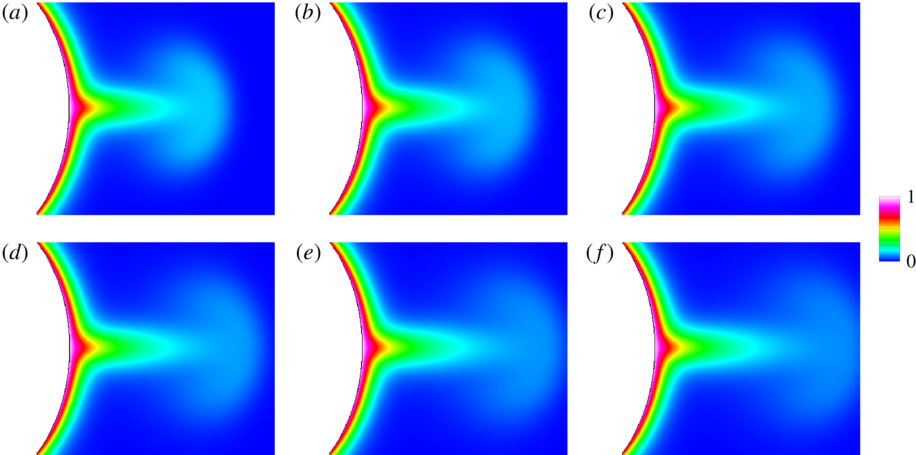
Contours of azimuthal velocity for a Reynolds number
 $Re=390$
for times (a)
 $t=15.8$
, (b)
 $17.1$
, (c)
 $18.3$
, (d)
 $19.6$
, (e)
 $20.8$
and (f)
 $22.1$
0.

Time-resolved particle image velocimetry (TR-PIV) of the flow was conducted. For PIV data acquisition, a laser sheet was generated perpendicular to the sphere (shown schematically in figure 1). Hollow glass spheres (density
 ${\approx}1.05~\text{kg}~\text{m}^{-3}$
, diameter
 ${\approx}10~\unicode[STIX]{x03BC}\text{m}$
) were used as tracer particles. The PIV system consisted of a 5 W CW Nd: YVO4 laser from Spectra-Physics Millenia and a Lumenera 4.0 Megapixel 90 f.p.s. USB3 camera mounted with a Tokina 100 mm,
 $f/2.8$
lens. Cropping of the active area of the camera sensor allowed for image capture rates up to
 $500$
f.p.s. The velocity flow field was obtained by cross-correlating 50% overlapping windows of
 $32\times 32$
pixels, or
 $16\times 16$
pixels depending upon the size of the active area of the camera sensor, yielding fields of up to
 $160\times 128$
vectors.
3 Results
3.1 A computational prelude to the experimental results
Before presenting our experimental data, we first present and discuss some results from an allied computational study of the (axisymmetric) flow around an impulsively rotated sphere. (In order to simulate a change in rotation rate of the sphere from
 $0$
, for
 $t\leqslant 0$
, to a constant rate
 $\unicode[STIX]{x1D6FA}$
, for
 $t>0$
, it is necessary to consider a frequency,
 $\tilde{\unicode[STIX]{x1D6FA}}(t)$
which changes from
 $0$
to the constant
 $\unicode[STIX]{x1D6FA}$
in a fixed time; for the computations reported here this was done using a simple linear variation over a ‘spin-up’ time of
 $t_{s}=0.05$
.) These calculations were obtained using a spectral-element discretisation of the flow domain (which was taken to be axisymmetric); the computational flow domain was chosen to mimic our experimental facility. Full details of the computational methodology have been reported elsewhere; see Calabretto et al. (Reference Calabretto, Levy, Denier and Mattner2015a
) and Calabretto, Mattner & Denier (Reference Calabretto, Mattner and Denier2015b
). In this section we will only present results which are pertinent to the discussion of our experimental data.
We solve this problem numerically using Semtex, a quadrilateral spectral-element direct numerical solver, whose capabilities are well suited to flows involving cylindrical coordinate systems (see Blackburn & Sherwin Reference Blackburn and Sherwin2004), and which is readily adapted to the spherical geometry considered here. For the problem to be computationally tractable, we first embed the sphere within a larger volume of fluid contained in a large, cylindrical container (thus mimicking our experimental tank). This allows us to apply full physical no-slip boundary conditions on all rigid surfaces (that is, the sphere surface and the bounding container). The computational container dimensions were suitably large so as to ensure that the outer rigid boundaries did not affect the flow dynamics, at least for the
 $O(1)$
times immediately following the spin-up and the subsequent boundary-layer collision.
To appropriately capture the behaviour of the boundary layer, we employ a fine mesh around the circumference of the sphere cross-section, containing a computational mesh of
 $36\times 36$
Lagrange knot points. This ensures that our computations are fully resolved and accurately capture the dynamics of the thin boundary layer; extensive tests were undertaken in this regard to ensure that all results presented here are converged to within graphical accuracy for the range of Reynolds numbers considered in this study. Extensive tests were undertaken to ensure that the flow induced by the rotating sphere was not affected by any interaction with the walls of the larger cylinder on the time scales we consider here. In all our calculations the temporal time stepping is accomplished via a second-order backwards-differencing scheme (see Blackburn & Sherwin Reference Blackburn and Sherwin2004); the time step
 $\unicode[STIX]{x0394}t$
was set to
 $5\times 10^{-4}$
, and convergence tests demonstrated that this was more than sufficient for our computations.
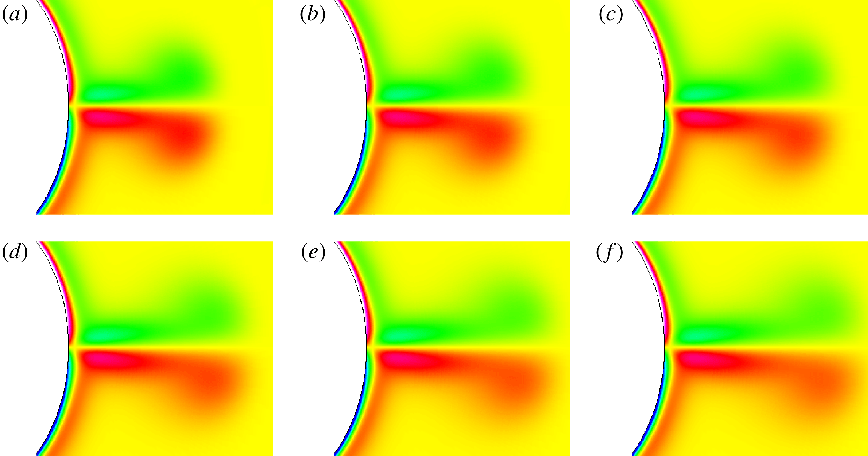
We present two sets of typical results from these computations, one relating to the azimuthal velocity and the second relating to the in-plane vorticity. Although our experimental set-up is unable to capture the azimuthal velocity, it still proves useful to consider the flow development in the context of the changes observed in the azimuthal velocity component. In order to provide validation against our experiments, we first present some results for a moderate Reynolds number,
 $390$
, which is chosen to coincide with the lowest value used in our experiments, see table 1. Figure 2 shows contour plots of the azimuthal velocity and figure 3 shows contour plots of the in-plane vorticity; all other components of vorticity are zero. (We note that our calculations are for Reynolds numbers lower than those predicted for the onset of three-dimensional instabilities in the boundary layer. For this reason, we have employed an explicit assumption of axisymmetry in all the calculations reported here.)
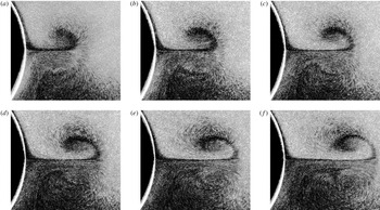
A number of important features of the flow can be observed in these images. With the imposition of angular motion to the sphere, fluid within the boundary layer is transported from the sphere’s poles to the equator where it collides to form a radial jet. This radial jet is headed by a starting vortex, which can clearly be seen in figures 2 and 3. The starting vortex propagates away from the sphere, leaving behind it a radial jet that remains (at least for this Reynolds number) symmetric about the equatorial plane. At suitably high Reynolds numbers, and hence not shown here, the starting vortex detaches from the radial jet and propagates outwards from the sphere as a toroidal vortex pair in which the azimuthal velocity has decayed to zero (see Calabretto et al. (Reference Calabretto, Levy, Denier and Mattner2015a
) for more detail on this aspect of the flow evolution). Additionally, computational study of Calabretto et al. (Reference Calabretto, Levy, Denier and Mattner2015a
) demonstrates that at higher Reynolds numbers the radial jet develops an absolute instability, which breaks the (initial) equatorial symmetry of the flow. This instability only occurs at suitably high Reynolds numbers, typically
 $O(10^{4})$
, and arises in the computations as a result of the accumulation of numerical round-off, which acts as a ‘small amplitude’ disturbance to the flow. We will return to this point later.
Contours of vorticity for a Reynolds number
 $Re=390$
for times (a)
 $t=15.8$
, (b)
 $17.1$
, (c)
 $18.3$
, (d)
 $19.6$
, (e)
 $20.8$
and (f)
 $22.1$
.

False streamline images of the flow showing the starting vortex. Each image is comprised of five separate images (taken at
 $0.25$
s intervals), overlaid to give the impression of particle motion, allowing the visualisation of instantaneous flow streamlines. Shown are results from times
 $t=$
(a)
 $15.8$
, (b)
 $17.05$
, (c)
 $18.3$
, (d)
 $19.55$
, (e)
 $20.8$
, (f)
 $22.05$
s after the initiation of sphere’s rotation. These correspond to a Reynolds number of
 $390$
.

3.2 Experimental results
There are four main structures observed, or predicted, by earlier works, namely (i) the boundary-layer collision that occurs at the equator after the initial spin-up (and which has been linked to a finite-time singularity in the boundary-layer equations), (ii) the subsequent eruption from the equator of a starting vortex and development of a radial jet, (iii) the development of an absolute instability within the jet and (iv) (perhaps most controversially) the prediction of a large
 $O(Re^{-1/2})$
recirculation zone in the vicinity of the jet equator. We now consider each of these aspects of the predicted flow, in turn, through our experimental results.
3.3 The boundary-layer collision and starting vortex
In figure 4 we present ‘false streamline’ images of the flow showing the starting vortex. These images were constructed by taking five separate images (at
 $0.25$
s intervals) and overlaying them to give the impression of particle motion (giving the impression of streamlines). The dimensions of the plots of the in-plane vorticity presented in figure 3 have been scaled so that they match the physical dimensions of the sphere in figure 4, thus allowing direct qualitative comparison between experiment and computation. Comparing these two images we see that the computational results accurately capture the developmental stages of the starting vortex and the radial jet, giving us confidence that our computational scheme is accurately capturing the flow dynamics. Close inspection of the images in figure 4 provides us with a first glimpse of the post-collision boundary layer/erupting jet region. We clearly observe a clean separation of the boundary layers from the surface, which then merge smoothly with the radial jet; there is no evidence of a recirculation zone on a scale comparable with the boundary-layer (or jet) thickness.
3.3.1 The time-averaged flow
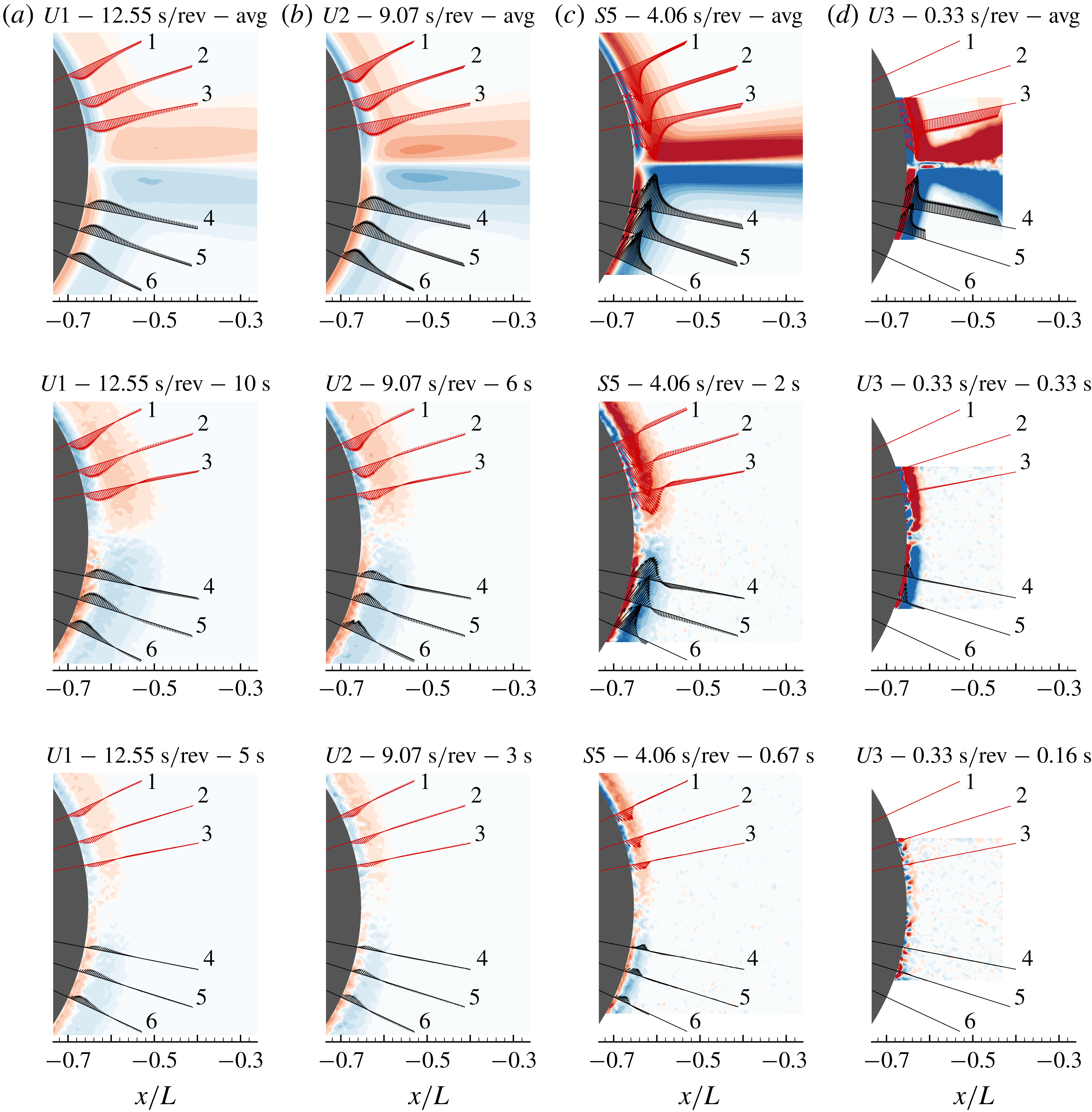
In order to further explore the dynamics of the flow, we now consider time-averaged velocities, extracted from the PIV data. Given that the flow is started from rest, it is important, when calculating the time-averaged velocity fields, to ensure that the initial time used in the time average is suitably large so as to ensure an accurate representation of the averaged quantities. (We note here that physical set-up of our camera and motor, controlling the rod/sphere assembly, did not allow for these to be synced. Thus, in all the experiments, image capture was begun prior to the start of the sphere’s rotation. By analysing the resulting images we were able to identify the clock time at which the sphere’s motion was initiated; all subsequent times quoted in the text were then determined from time stamps embedded in each image.) Results for this time-averaged velocity and vorticity are shown in figure 5 (for four different Reynolds numbers; see table 1). For the three lowest Reynolds numbers, the time-averaged vorticity exhibits the same double-layered structure near the sphere’s surface as seen in the computational results of figure 3, again showing no evidence of any recirculation zones near the equatorial plane. The results for increasing Reynolds number also show an intensification of the vorticity near the sphere and a thinning of the radial jet and the boundary layer on the sphere’s surface (as both must scale with
 $Re^{-1/2}$
). The last of these images, figure 5(d), which corresponds to a Reynolds number
 $Re=14\,750$
, shows clear evidence of the jet instability that has developed, and which can be seen to have propagated back towards the sphere’s equator. There is also evidence in this image of a secondary vortex, centred on the equator, but outside the boundary layer. We conjecture that this vortex is a result of the competition between the flow out from the sphere, in the radial jet, and the flow back towards the sphere from the jet instability (which propagates upstream against the outward radial direction of the mean jet flow).
Contours of instantaneous vorticity, with superimposed instantaneous velocity field, for a variety of final rotation rates and times (see table 1). The four series are for (a)
 $\unicode[STIX]{x1D6FA}=2\unicode[STIX]{x03C0}/12.55~\text{rad}~\text{s}^{-1}$
(
 $Re=390$
) (b)
 $\unicode[STIX]{x1D6FA}=2\unicode[STIX]{x03C0}/9.07~\text{rad}~\text{s}^{-1}$
(
 $Re=540$
) (c)
 $\unicode[STIX]{x1D6FA}=2\unicode[STIX]{x03C0}/4.06~\text{rad}~\text{s}^{-1}$
(
 $Re=1200$
) and (d)
 $\unicode[STIX]{x1D6FA}=2\unicode[STIX]{x03C0}/0.33~\text{rad}~\text{s}^{-1}$
(
 $Re=14\,750$
) with times as noted. The top image in each series shows the average vorticity and velocity field.

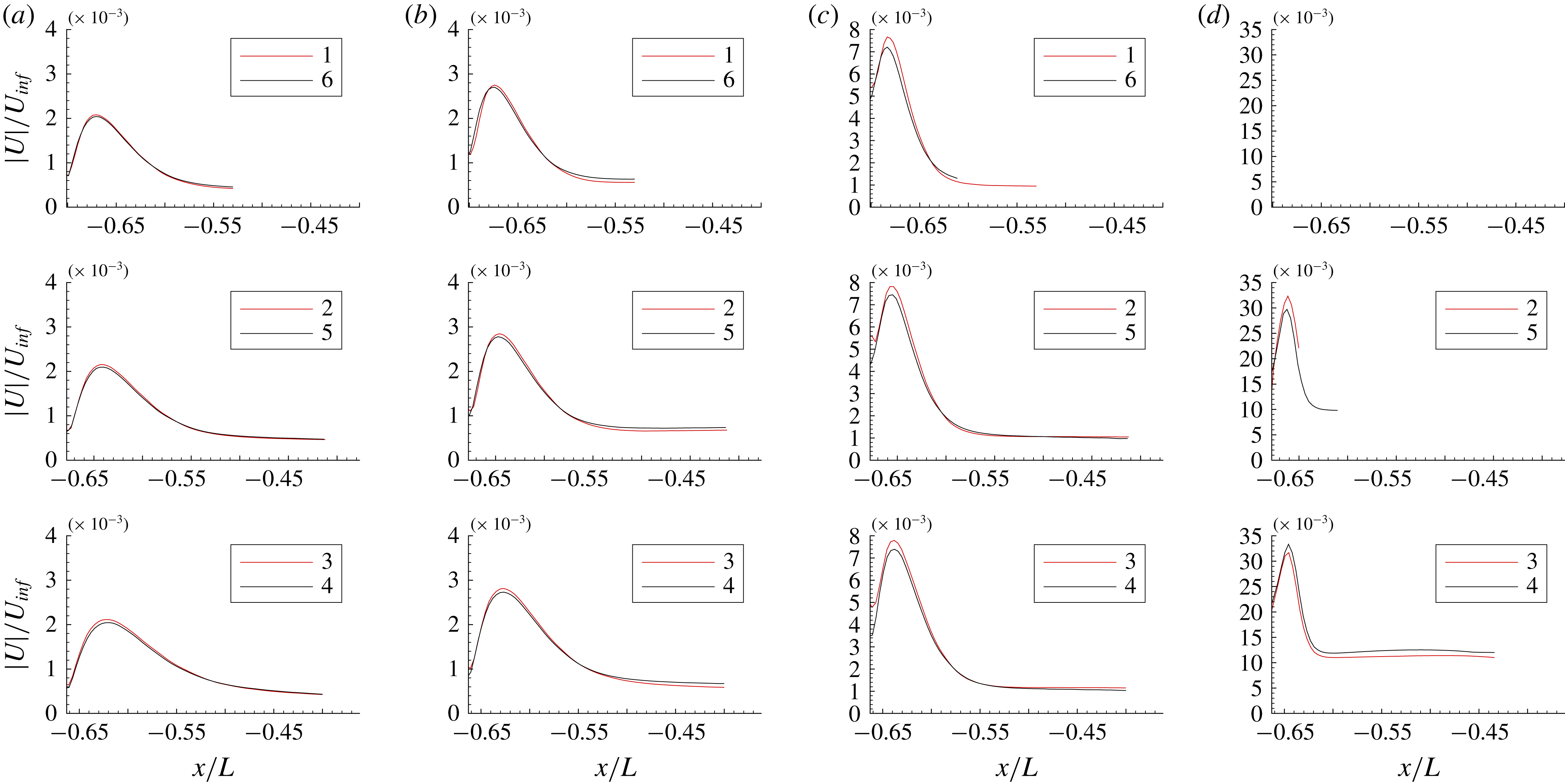
Plots of the time-averaged velocity for Reynolds numbers (a)
 $390$
, (b)
 $540$
, (c)
 $1200$
and (d)
 $14\,750$
at locations
 $1,2,\ldots ,6$
as indicated in figure 5. For the case shown in (d), the camera aperture did not allow capture of data at locations
 $1$
and
 $6$
.

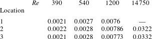
The time-averaged velocity profiles, measured outwards from the sphere at the locations marked in figure 5, can be extracted from our experimental data; these are presented in figure 6. We note that the averaging process has been done for times after the starting vortex has developed and been ejected. The most noticeable feature in these plots is the fact that there is no evidence of a recirculation zone adjacent to the sphere’s surface. Together with the (approximate) top/bottom symmetry of the flow around the equatorial plane, this further serves to demonstrate that the colliding boundary layers separate smoothly from the sphere at the equator. The maximum velocity, extracted from the data presented in figure 6, is given in table 2. The amplitude of the velocity clearly grows with increasing Reynolds number, however, we are unable to identify any characteristic scaling for the velocity from this limited data. Finally, we note that, at the highest Reynolds number (see figure 6 d) this top/down symmetry is broken due to the aforementioned instability in the radial jet.
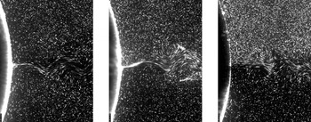
Instantaneous images of the flow captured with a reduced camera aperture, allowing a capture speed of
 $229$
f.p.s. Shown are images, for a flow Reynolds number of
 $14\,750$
, taken
 $13.62$
,
 $15.28$
and
 $42.92$
s after the sphere has been impulsively rotated from rest.

Maximum velocity extracted from the time-averaged velocities at locations 1, 2 and 3 shown in figure 6.

3.4 The jet instability
Images of the averaged velocity field, presented in figure 5(d), show clear evidence of a symmetry breaking instability in the radial jet. This instability is also seen in the experiments of Hada & Ito (Reference Hada and Ito2003) and conjectured by Bowden & Lord (Reference Bowden and Lord1963) to be the cause of the shortening of the jet they observed in their schlieren photographs. This instability is also clear in the axisymmetric computations of Calabretto et al. (Reference Calabretto, Levy, Denier and Mattner2015a ), although in their computations, the instability develops only at higher Reynolds numbers than those for which it was observed by Hada & Ito (Reference Hada and Ito2003) and in our present experiments.
By undertaking a classical stability analysis of the (local) boundary layer on the sphere, Garret & Peake (Reference Garret and Peake2002) found that the flow in the boundary layer is stable to spiral instabilities when the Reynolds number is below
 $11\,000$
(or thereabouts). This would therefore seem to preclude these spiral vortices as being the culprits for the onset of the jet instability in Bowden’s experiments, where the ‘instability’ is observed (through a shortening of the jet) at a Reynolds number of
 ${\approx}2000$
, and in Hada & Ito’s experiments at Reynolds numbers as low as
 $2600$
(see their figure 5). This would seem to negate Hada & Ito’s (Reference Hada and Ito2003) conjecture as to the instability mechanism. At the highest Reynolds number of our experiments,
 $Re=14\,750$
, the jet instability can clearly be seen from the three images presented in figure 7. These instantaneous images of the flow were captured using a reduced camera aperture, allowing for a capture frame rate of
 $229$
f.p.s. The jet instability propagates back towards the sphere surface as time progresses; in the last of these images we can see a classical von Kármán vortex street. We note here that although our highest Reynolds number is larger than that predicted by Garret & Peake (Reference Garret and Peake2002), and so one would expect the boundary-layer flow away from the equator to develop spiral vortices, we found no evidence of this in any of our experimental data. One possible reason for this is that the sphere(s) we have employed in our experiments are ‘smooth’ (the pool balls we used are manufactured to a very high tolerance and have a measured ‘local roughness’ of approximately
 $1~\unicode[STIX]{x03BC}\text{m}$
, compared to the ball radius of
 $28\,560~\unicode[STIX]{x03BC}\text{m}$
(see Alciatore Reference Alciatore2018)). There therefore seems to be little opportunity for the spiral vortices to be triggered in our experiments through, for example, a roughness induced receptivity mechanism. (A similar series of experiments were also undertaken in the early 1960s by Kreith et al. (Reference Kreith, Roberts, Sullivan and Sinha1963). This set of experiments used a smooth ebonite bowling ball, with a diameter of
 $21.83$
cm and roughness no greater than
 $0.0006\,\%$
of the ball’s diameter. Kreith et al. conclude by noting that at ‘Reynolds numbers below
 $Re_{d}=5\times 10^{5}$
the flow induced by a sphere rotating in an infinite environment is laminar except for a small region in the vicinity of the equator where the boundary layers from the two halves of the sphere meet’.)
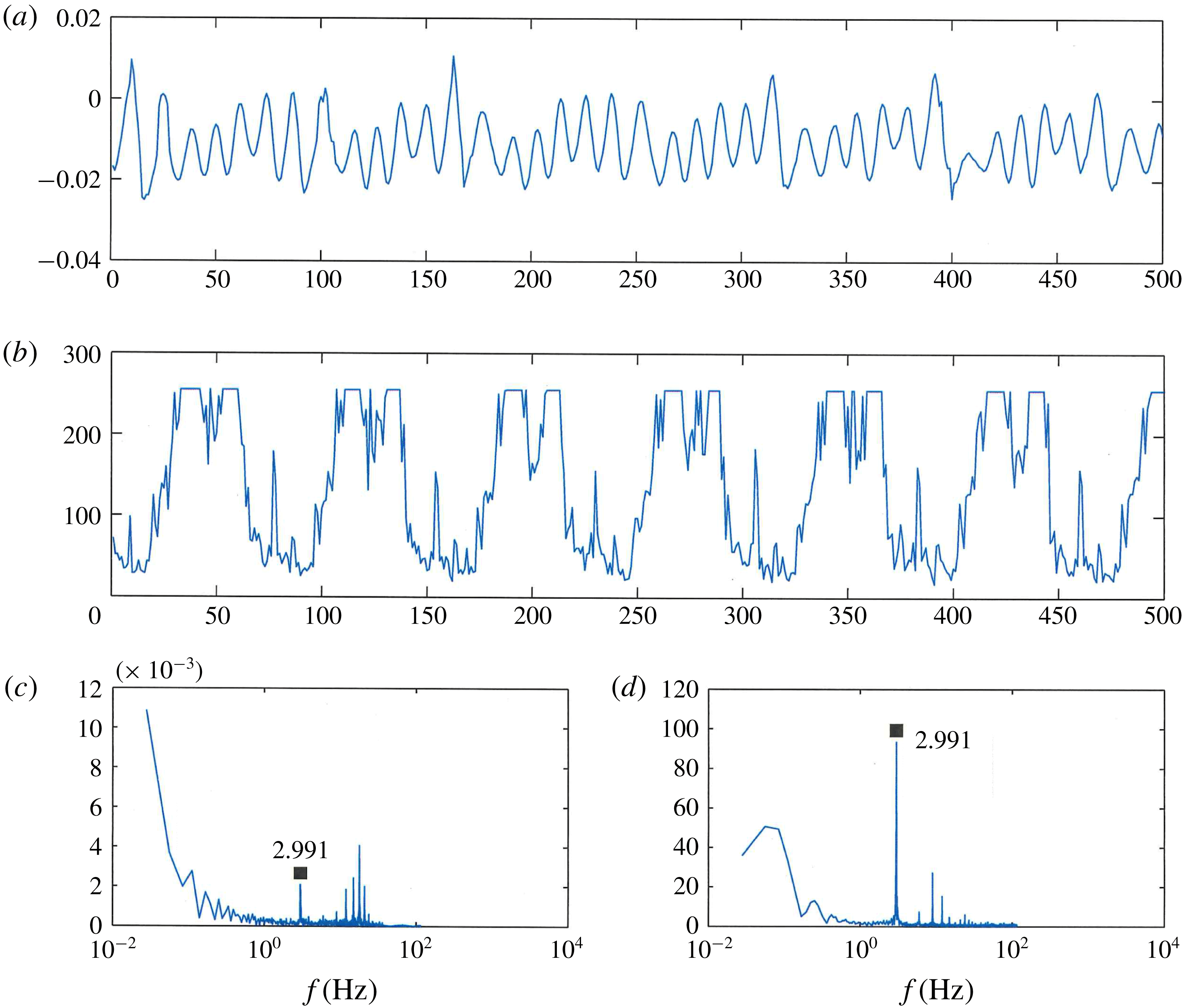
Plots of the (a) jet velocity (measured in the radial direction, along the equator), (b) the sphere precession (measured in
 $\unicode[STIX]{x03BC}\text{m}$
), the single-sided spectrum
 $|Y(f)|$
of the (c) jet velocity and (d) the sphere precession versus frequency.

These facts then suggest that another mechanism is at play in providing the receptivity mechanism for the onset of this jet instability. In order to explore this issue further we recall that in our experimental set-up, the rod/ball system, although manufactured to very high tolerances, exhibits some degree of error; although the rod defines the axis of rotation of the sphere, the rod is not perfectly centred from pole to pole. This error manifests as a slight precession of the sphere around its (nominal) perfect vertical location, which could then serve as a driving mechanism for the instability (see § 2 for details). To test this conjecture we calculated the spectral frequencies of the jet instability and these are shown in figures 8 and 9. Figure 8 shows a plot of the jet velocity, extracted from our experimental data for the case of a Reynolds number of
 $Re=14\,558$
, together with a plot of the sphere precession, measured by observing the change in location of the sphere’s surface (at the equator) with time. (These locations were extracted from the experimentally captured images by identifying the pixel that coincided with the outer edge of the sphere. The sampling frequency was 229 Hz. The ‘flat tops’ seen in figure 8(b) are a consequence of the fact that we cannot visually differentiate the location of the sphere to an accuracy of better than one pixel over such a short time period (
 ${\sim}0.004~\text{s}$
).) We can extract the single-sided power spectrum from each set of measurements, which allows us to identify the dominant frequency in the jet fluctuations and also within the precession. These are shown in figure 8. A comparison of the single-sided amplitude spectrum of the jet fluctuations with that of the sphere precession shows a clear correlation between the frequency of precession, which is simply the frequency of rotation, with that of the jet instability. Further evidence of the effect of the jet precession on the instability can be seen in figure 9, where we again present the frequency spectrum extracted from the measurements of the jet velocity on the equatorial plane, for a slower rotation rate (of
 $0.57$
rev/sec, or
 $Re=2774$
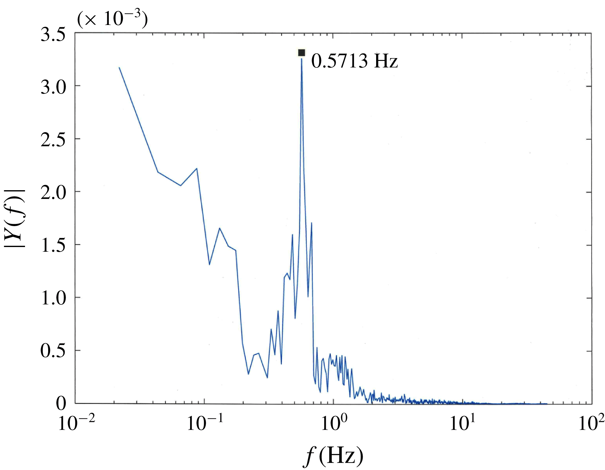
). Even at this moderate Reynolds number, there is clear evidence of the instability, identified through the dominant frequency in the radial jet, which is locked to the rotation rate of the sphere. This evidence strongly points to the jet instability being forced, or driven, by any small asymmetries that might exist within the experimental apparatus.
Frequency spectrum extracted from the jet velocity (measured on the equator), at a lower rotational speed of
 $0.57$
rev/sec (corresponding to a Reynolds number of
 $Re=2774$
). Note the dominant frequency of the instability matches that of the rotation rate of the sphere, hence confirming that the instability is locked in with the small precession measured in the sphere rod system.

4 High-Reynolds-number computations
We now turn our attention to the other major aspect of the post-collisional flow that has, to date, avoided explanation. This is related to the conjectured steady flow that connects the boundary layer on the sphere to the radial jet. Two explanations, each based upon a high-Reynolds-number asymptotic description of the flow in this region, have been put forward. The first, due to Stewartson (Reference Stewartson and Görtler1958), conjectures a two-layer structure, with an outer region of thickness
 $O(Re^{-1/2})\times O(Re^{-1/2})$
, based upon distance from the sphere’s surface and angle from the equatorial plane, in which the flow smoothly detaches from the sphere, joining smoothly with the radial jet (see the schematic presented in Stewartson’s figure 1). Stewartson also conjectures that the radial velocity changes sign in the boundary-layer region, but that the region over which this occurs is small. (Stewartson (Reference Stewartson and Görtler1958) also notes that a second, inner boundary layer is required to complete the flow description, but also notes that the flow within this boundary layer is ‘negligible in comparison with the velocity in the outer inviscid layer’.) Smith & Duck (Reference Smith and Duck1977) propose a different structure, which exhibits a large-scale recirculation zone in the region around the equator, where the fluid from the two boundary layers collides (see the schematic presented in Smith & Duck (Reference Smith and Duck1977) figure 6b).
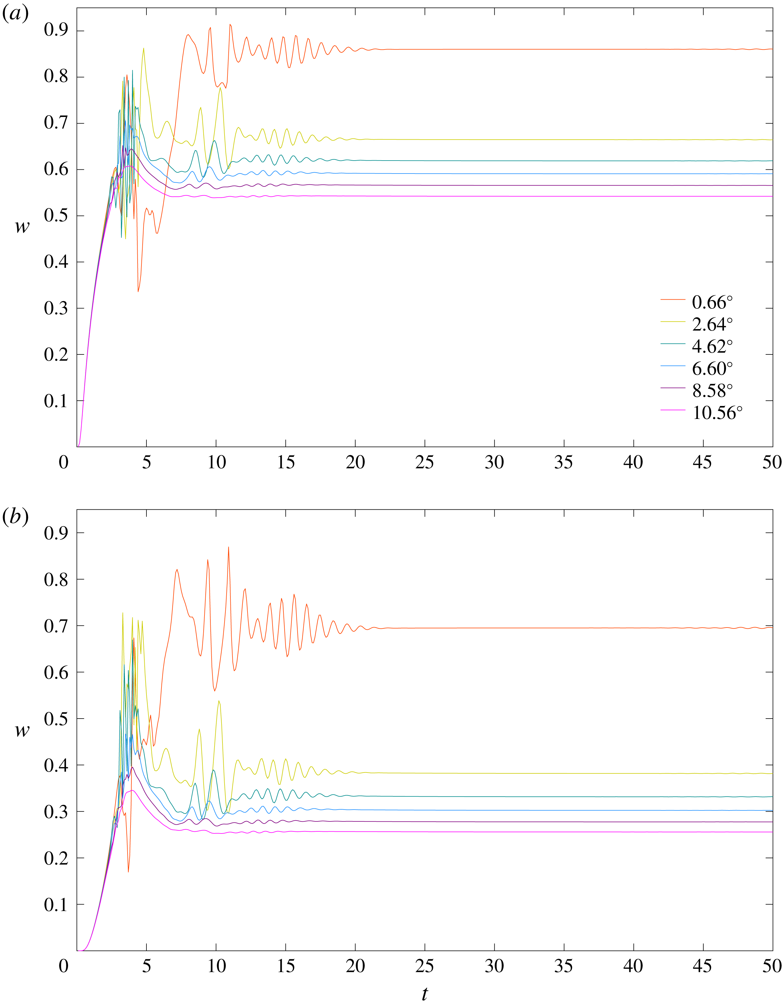
Plots of the azimuthal velocity
 $w$
versus time at a radial position of (a)
 $r=0.005$
, and (b)
 $r=0.01$
, and at different angles from the equator (located at
 $\unicode[STIX]{x1D703}=0$
) for a flow Reynolds number
 $Re=10^{5}$
.

Contour plots of the radial velocity
 $u$
for flow Reynolds numbers (a)
 $Re=10^{4}$
, (b)
 $Re=2\times 10^{4}$
, (c)
 $Re=4\times 10^{4}$
and (d)
 $Re=8\times 10^{4}$
.

Our experimental results show no evidence of the recirculation zone conjectured by Smith & Duck (Reference Smith and Duck1977). This result is rather surprising, noting that, although the results of Smith & Duck (Reference Smith and Duck1977) are based upon a high-Reynolds-number asymptotic description of the flow, one would reasonably expect that the theory would provide at least qualitative agreement even for the moderate Reynolds numbers of our experiments. Our experiments do not provide direct confirmation of Stewartson’s (Reference Stewartson and Görtler1958) conjectured structure, although we note that the small region of reversed flow posited by Stewartson may not be resolved in our experiments, which were initially conceived to explore the larger scale, global, behaviour of the flow. One possible reason for this discrepancy may lie in the fact that for the high-Reynolds-number description of the flow to appear, one must take the experiments to appropriately high Reynolds numbers. Unfortunately, in the context of our experiments, the advent of the absolute instability in the jet (due to the, albeit, very slight precession in the experimental apparatus) precludes this. The development of this instability in the radial jet also posses significant challenges if we wish to explore the large Reynolds number structure of the boundary layer in the vicinity of the equator (that is, where the boundary layer detaches from the sphere); at suitably high Reynolds numbers, the jet has become unstable (indeed, the jet’s motion will likely be fully turbulent) presenting a considerable computational challenge to fully resolve the turbulent flow.
In order to overcome this, and provide a tractable computational problem, we must suppress the jet instability. This is most readily done by noting that the jet instability serves to break the flow symmetry. From the perspective of the global flow, the jet instability can be seen as a symmetry breaking bifurcation; in the mathematical sense, the symmetric flow (consisting of the boundary-layer and steady jet regions) becomes unstable at a critical Reynolds number, leading to a new dynamical state. In the context of a dynamical system approach, our computational tasks then reduces to calculating an unstable solution of the axisymmetric Navier–Stokes equations for the flow due to the sphere that exhibits symmetry about the equator. We can achieve this by imposing symmetry at the equator
 $$\begin{eqnarray}\frac{\unicode[STIX]{x2202}u}{\unicode[STIX]{x2202}z}=v=\frac{\unicode[STIX]{x2202}w}{\unicode[STIX]{x2202}\unicode[STIX]{x1D719}}=0\quad (\text{on }z=0),\end{eqnarray}$$
and restricting our computational domain appropriately. The flow domain is then discretised using the spectral-element method semtex (see Blackburn & Sherwin Reference Blackburn and Sherwin2004). In order to explore the theorised steady-state solution, the computational scheme is marched forward in time from
 $t=0$
until a steady-state solution is achieved. An example of the approach to this steady-state solution is given in figure 10, where we show the azimuthal velocity versus time at various radial distances from the sphere’s surface for a flow Reynolds number of
 $Re=10^{5}$
; note that these radial positions are within the boundary layer. For suitably large times, we clearly see the development of a steady state. Prior to this, the computed flow shows a series of developing disturbances that propagate towards the equator. We make the important point here that at these large Reynolds numbers,
 $O(10^{5})$
or higher, these instabilities are not physical. The full physical flow would have become fully turbulent by this point, and indeed, undergone a ‘symmetry breaking bifurcation’, in the form of an absolute instability of the radial jet at a lower Reynolds number.
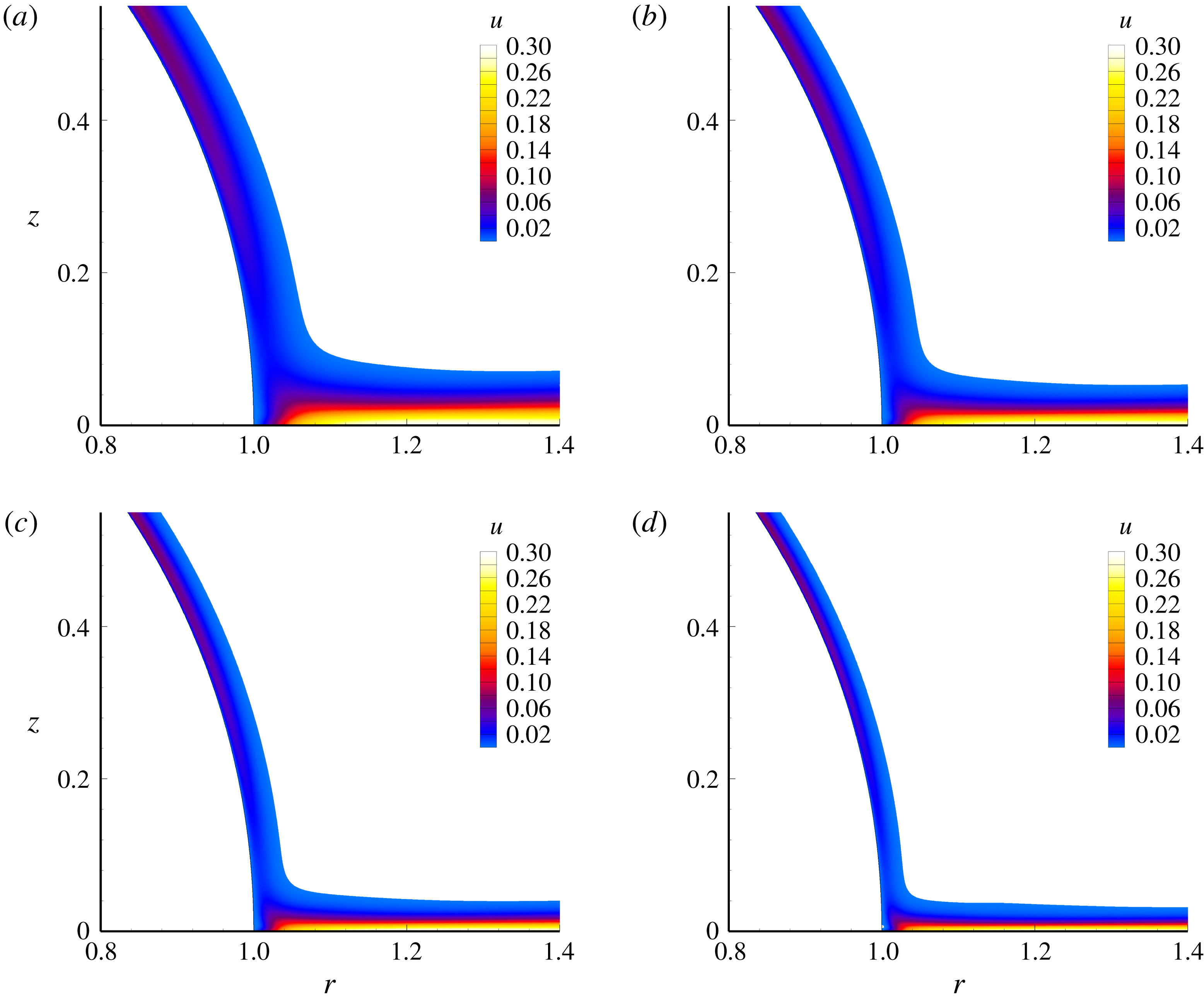
Turning now to the question of the large-Reynolds-number steady state, we present in figure 11 contour plots of the radial velocity for a range of Reynolds numbers. The contour levels have been chosen so that a coloured region indicates a region of positive radial velocity. The boundary layer is clearly observed, as is the radial jet emanating from the origin. For these Reynolds numbers, and at this scale, there is no evidence of a region of recirculation adjacent to the sphere’s surface. We note that Stewartson’s model for the equatorial region, where the boundary-layer assumption on the sphere’s surface breaks down, is of
 $O(Re^{-1/2})$
, leading to an
 $O(Re^{-1/2})\times O(Re^{-1/2})$
region at the equator–sphere surface junction.
Stewartson’s analysis requires an additional inner, viscous layer of thickness
 $O(Re^{-3/4})$
. Smith & Duck’s analysis predicts a clear recirculation zone, of thickness
 $O(Re^{-3/14})\times O(Re^{-3/14})$
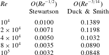
, at the equator–sphere surface junction. To provide some context to these scalings, we present some numerical values for various Reynolds numbers in table 3. It seems clear from the results presented in figure 11 that Smith & Duck’s
 $O(Re^{-3/14})$
-thick recirculation region does not exist. The
 $O(Re^{-1/2})$
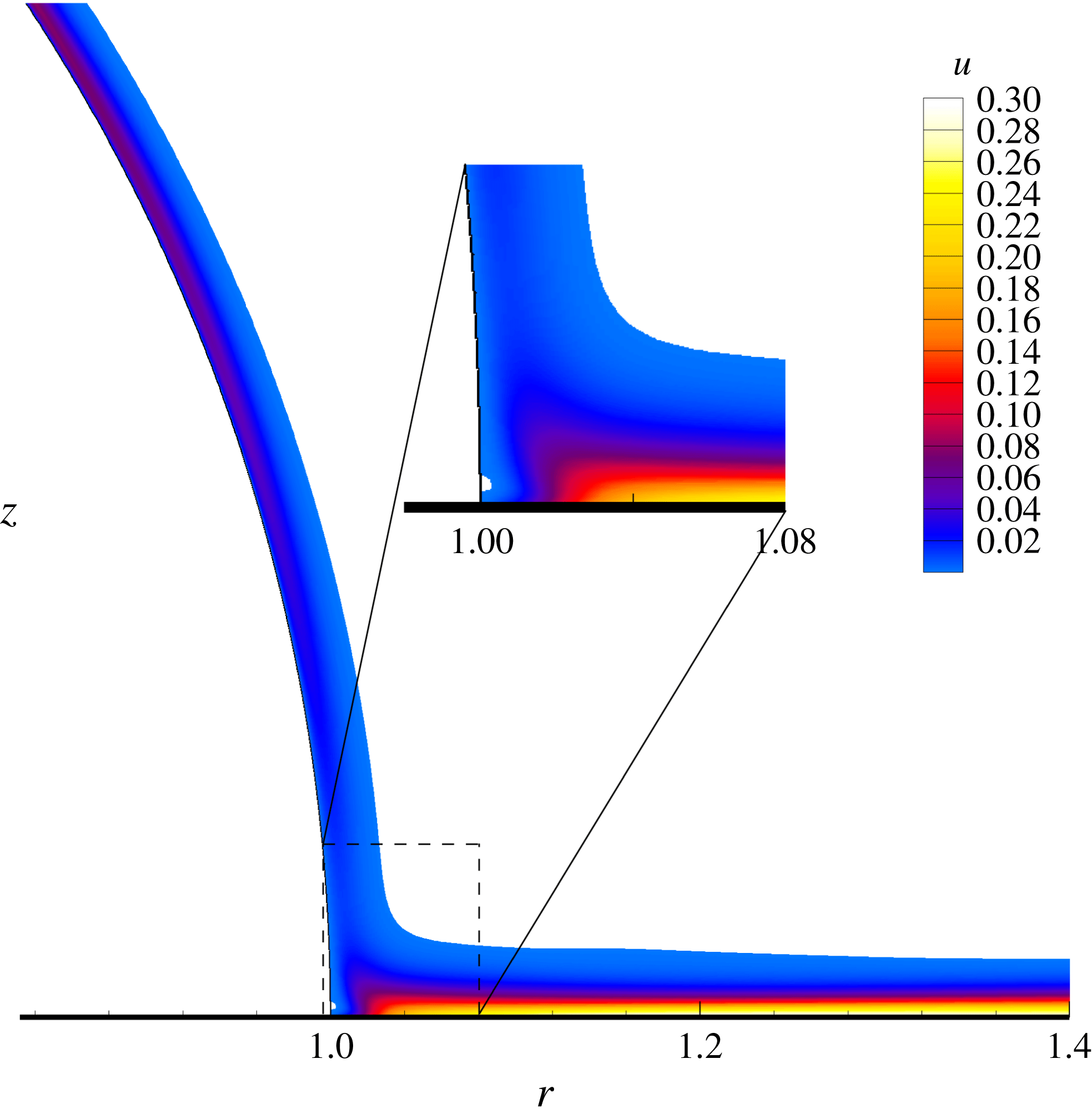
scalings of Stewartson’s predict a much smaller region in which one would expect to observe reversed flow. There is little evidence of this reversed flow, at this scale, in figure 11. However, zooming in on the region near the equator, as has been done in figure 12, for the case of
 $Re=O(10^{4})$
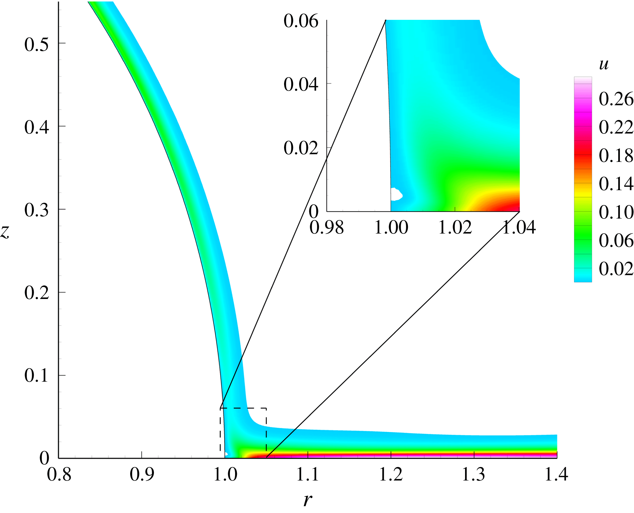
, we see the emergence of a (very) small region in which the radial velocity is negative (observe the small white patch seen in the inset). This is more clearly seen in contour plots of radial velocity, at
 $Re=10^{5}$
, presented in figure 13. The region of negative radial velocity (that is, recirculating flow) is more pronounced, but still small.
Two clear points can be drawn from the images in figures 11–13. The first is that no large-scale recirculation, as posited by Smith & Duck, exists in this flow. The second is that there is a small region of recirculation in the vicinity of the equatorial plane, but it is centred on the equator. The latter is in qualitative agreement with Stewartson who states, in reference to his equation (1.9), that ‘the flow must separate somewhere’ and that the ‘separated region is confined to the vicinity of
 $\unicode[STIX]{x1D701}=0$
’ (
 $\unicode[STIX]{x1D701}=0$
denoting the equator in Stewartson’s notation). The results of our computation therefore suggest that the structure proposed by Stewartson is, qualitatively, correct.
Contours of the radial velocity, for the case
 $Re=8\times 10^{4}$
, and inset, a zoomed image, near the equator. The contours have been set so that a positive radial velocity presents as a colour (with magnitude identified by the associated colour map). The dimension of the zoomed area correspond to a physical dimension of
 $2.3$
mm for a sphere of diameter
 $57.15$
mm.

Numerical estimates for the layers predicted by the Stewartson (Reference Stewartson and Görtler1958) and Smith & Duck (Reference Smith and Duck1977) analyses.

Contours of radial velocity, for the case
 $Re=10^{5}$
, and inset, zoomed image, near the equator. The contours have been set so that a positive radial velocity presents as a colour (with magnitude identified by the associated colour map). The dimension of the zoomed area correspond to a physical dimension of
 $1.14$
mm for a sphere of diameter
 $57.15$
mm.

5 Conclusions
We have presented new experimental results of the flow around a sphere, immersed in an otherwise quiescent body of fluid, which is spun from rest to a constant angular velocity. The development of the viscous boundary layer, its subsequent collision and eruption from the sphere’s surface as a jet at the equator has been demonstrated, and our experimental results show good qualitative agreement with computational results. The jet instability, which has been shown to develop in the axisymmetric calculations of Calabretto et al. (Reference Calabretto, Levy, Denier and Mattner2015a ), is seen experimentally at much lower Reynolds numbers than predicted by the axisymmetric calculations. Similar results were observed in the experiments of Hada & Ito (Reference Hada and Ito2003) and inferred in the much earlier experiments of Bowden & Lord (Reference Bowden and Lord1963). Our results demonstrate an alternative driving mechanism for the generation of the jet instability at lower Reynolds numbers, with the forcing (or receptivity mechanism) provided by the precession that occurs in our experimental apparatus due to the slight (less than 0.4 %, based upon sphere radius) in positioning of the rod through the sphere’s poles. The precise frequency locking between the sphere precession and the jet shedding frequency provide clear confirmation of this. We note that the experimental apparatus of Hada & Ito (Reference Hada and Ito2003) also has the potential to introduce a similar symmetry breaking, given that their sphere is mounted only at one pole.
In all of our experiments, we have found no evidence of the spiral vortices found in the experiments of Kohama & Kobayashi (Reference Kohama and Kobayashi1983), even though our experimental Reynolds numbers span the range at which spiral vortices are predicted to exist. As discussed in § 3.4, our sphere is very smooth, thus limiting the potential for a roughness induced receptivity mechanism to generate spiral vortices. Similar results were also found by Kreith et al. (Reference Kreith, Roberts, Sullivan and Sinha1963), who used an ebonite bowling ball and noted that at ‘Reynolds numbers below
 $Re_{d}=5\times 10^{5}$
the flow induced by a sphere rotating in an infinite environment is laminar except for a small region in the vicinity of the equator where the boundary layers from the two halves of the sphere meet’. Furthermore, potential ‘free-stream’ disturbances to the sphere’s boundary layer are also limited due to the fact that our experiments were conducted in a water tank, which was mounted on a table designed to minimise external vibrations.
Having designed our experiments so as to minimise all potential receptivity mechanisms, through either surface roughness or those introduced through the fluid itself, we found no evidence of spiral vortices, even though our experiments were conducted at higher Reynolds numbers than the critical
 $Re$
for the instability, as predicted by linear stability theory. Recent work by Calabretto & Denier (Reference Calabretto and Denier2019) has provided some further insight into the sphere’s instability mechanism by showing that disturbances introduced into the flow are advected down to the equator through the sphere’s boundary layer, and then out into the radial jet, leaving a laminar boundary layer along most of the sphere’s surface for Reynolds numbers up to
 $O(10^{5})$
. In the (somewhat) related rotating-disk flow, Thomas & Davies (Reference Thomas and Davies2018) have recently demonstrated that the rotating-disk flow is globally unstable for suitably large
 $Re$
and
 $n$
(here
 $n$
is the azimuthal wavenumber of a linearised disturbance in the rotating-disk boundary layer); see their figure 17. It is possible that a similar global instability exists in the sphere flow, however, as demonstrated by Calabretto & Denier (Reference Calabretto and Denier2019), a lower bound on the critical Reynolds number for such an instability would necessarily need to be larger than those values shown by Calabretto & Denier (Reference Calabretto and Denier2019) to lead to convective instabilities. Further investigation of this issue is clearly required.
The last important point arising from our combined experimental and computational study concerns the fate of the boundary layers on the sphere after they collide. There is no evidence, in either our experiments or computations, of the large-scale separation region predicted by Smith & Duck (Reference Smith and Duck1977). Our large-Reynolds-number computations do show a (very) small region of reversed flow adjacent to the equatorial plane and, generally, in a location suggested by Stewartson’s analysis. What is most surprising is that all attempts, of which we are aware, at providing a numerical solution of Stewartson’s outer, inviscid equations have not been successful (P. W. Duck, private communication 2019; S. J. Garrett, private communication 2019). That the, albeit small, separation region exists is clear from our results, adding weight to Stewartson’s analysis. However, the lack of appropriate solutions to Stewartson’s outer equations calls into question Stewartson’s belief that the separated region does not seriously modify the flow described by his outer, inviscid, equations. Although our new results have shed light on the post-singularity structure, the resolution to this long standing problem of the precise nature of the flow that results from the collision of two boundary layers remains open, and is the subject of ongoing work.
An alternative interpretation could be made to explain the small separation region seen in figures 12 and 13 (this was suggested to us by an anonymous referee). It is perhaps not well known that, under suitable conditions, Taylor–Görtler vortices can develop in a wall jet over a convex wall (Floryan Reference Floryan1986; Wadey Reference Wadey1992). The aforementioned works demonstrate theoretically that, for sufficiently large (negative) Görtler numbers (defined in the usual way as
 $2Re^{1/2}\unicode[STIX]{x1D6FF}$
, where
 $\unicode[STIX]{x1D6FF}$
is a measure of the surface curvature), counter-rotating Taylor–Görtler vortices can develop in a wall jet. The flow engendered by the sphere’s rotation has some similarities to a classical wall jet, but with the added complexity of the induced azimuthal velocity component. Some comparison, albeit qualitative, therefore seems possible. The two most important characteristics of Görtler vortices, pertinent to our discussion, are that their wavelength, and wall normal extent, scale with the boundary-layer thickness and that they appear as counter-rotating vortex pairs. Neither of these characteristics are evident in our numerical results (see figures 12 and 13). We conclude that the recirculation zone is not a manifestation of a steady Taylor–Görtler instability.
We close by noting that our PIV experiments may not be the final word in exploring the instability of the flow around (very) smooth rotating spheres. As noted by an anonymous referee, hot-wire anemometry, such as used to great effect in the rotating-disk experiments of Lingwood (Reference Lingwood1996) provide the opportunity to explore the flow structure with greater accuracy. We have plans to conduct such a series of experiments and hope to be able to report on them in the future.
Acknowledgements
S.A.W.C. and J.P.D. benefited from a number of useful discussions with Professor P. Duck. We are also grateful to the three anonymous referees, whose comments helped improve this manuscript.