1. Introduction
Autonomous navigation system is a critical capability for automated guided vehicles (AGVs) operating in indoor environments, such as industry manufacturing plants [ Reference Chung9,Reference Graba, Amamou, Kelouwani, Allani, Zeghmi, Agbossou and Mohammadpour18,Reference Keith and La21,Reference Zhang, Chen and Guo43], warehouses, and logistics centres. These environments often present complex and dynamic conditions, requiring vehicles to efficiently navigate through narrow aisles, avoid unexpected obstacles, and reach designated locations with high precision [Reference Yadegar, Kashi, Ghaderi, Meskin and Noorizadeh38]. The demand for robust and reliable indoor vehicle navigation systems has grown significantly, as well as in outdoor environments [ Reference Sun, You, Qiu, Wu, Xiong, Song, Zhang and Lu33,Reference Zhang, Yang, Wang, Guan, Ding and Lee42].
According to the survey [Reference Aizat, Azmin and Rahiman2], current AGV navigation systems mostly rely on conventional approaches such as line follower, optical guidance, inductive wire, magnetic spot, and laser guided with reflectors, which ensures precision of movement and positioning, but requires extensive hardware installation on each path. However, it only relies on predefined paths and local motion behaviours, which may be insufficient in dynamic and cluttered environments.
Furthermore, the vehicle is unable to avoid an obstacle and may become trapped in a deadlock location [ Reference Lee and Park24,Reference Nishida and Nishi29]. To overcome these challenges, the navigation systems must complete with global and local motion planning that integrates path planning, path tracking, and real-time obstacle avoidance within a single coordinated framework. To achieve autonomy, a system must have four key elements: perception [ Reference Da, Chen, Song and Lu10,Reference un Nabi Jafri, Iqbal, Khan and Chellali20,Reference Yue, Zhang, Chen, Chen, Zhou and He41], localisation [ Reference Deshmukh, Hasamnis, Kulkarni and Bhaiyya11,Reference Melvin, Wang and Yazdani26,Reference Yilmaz and Temeltas40,Reference Zohaib, Pasha, Javaid, Salaam and Iqbal46], path planning [ Reference Hichri, Gallala, Giovannini and Kedziora19,Reference Zohaib, Pasha, Javaid and Iqbal45], and motion control [ Reference Chai, Niu, Carrasco, Arvin, Yin and Lennox8,Reference Liu, Hua, Deng, Meng, Huang, Hu, Song, Gao, Liu, Shuai, Khajepour, Xiong and Xia25]. There should not be a single element left out to make a navigation system work in autonomous capabilities.
1.1. Related works
The focus of this research is on two key elements of autonomous navigation systems: path planning and motion control for ground vehicles, often referred to as mobile robots. Path planning functions as a global planner that generates waypoints for the vehicle to reach its destination, while motion control serves as a local planner that guides the vehicle along these waypoints.
The Probabilistic Roadmap (PRM) algorithm is a sampling-based method widely used for path planning in complex environments [ Reference Ayawli, Dawson, Badu, Ayawli and Lamusah6,Reference Yang, Li, Qian, Quan, Miao, Liu, Hu and Memetimin39]. It constructs a graph of feasible paths by randomly sampling the configuration space, allowing the vehicle to navigate efficiently through intricate areas [ Reference Geraerts and Overmars17,Reference Koller23]. However, PRM alone does not guarantee precise path following in real-world applications, where high trajectory accuracy is essential [Reference Thrun35]. Recent studies have emphasised the robustness of PRM in dynamic environments and its suitability for autonomous ground vehicle navigation [ Reference Ravankar, Ravankar, Emaru and Kobayashi31,Reference Tao, Daichuan, Weifeng, Chenglin and Baigen34]. Furthermore, several modified PRM approaches have demonstrated enhanced computational efficiency and adaptability under real-world operating conditions [ Reference Fareh, Baziyad, Rabie and Bettayeb14,Reference Francis, Faust, Chiang, Hsu, Kew, Fiser and Lee15].
Qiao et al. [Reference Qiao, Luo and Luo30] proposed an enhanced path planning algorithm for mobile robots navigating intricate environments with narrow passages. The algorithm improves upon the traditional PRM method by integrating the Artificial Potential Field (APF) algorithm to optimise the distribution and density of sampling points within confined areas.
Zhou et al. [Reference Zhou, Lu and Lv44] proposed an innovative approach to enhance path planning for AGVs operating in complex environments. The Grid-based Non-uniform Probability Density Sampling Probabilistic Roadmap (GN-PRM) algorithm addresses the limitations of conventional PRM methods in navigating narrow passages by incorporating grid-based map segmentation and non-uniform probability density sampling. This approach improves sampling density in confined regions while optimising computational efficiency.
For motion control, the Pure Pursuit (PP) algorithm is an effective path-tracking method that computes steering commands to enable a vehicle to follow a predefined trajectory smoothly and accurately [Reference Aizat, Qistina and Rahiman4]. The integration of PP into mobile robot and ground vehicle systems has been extensively studied, demonstrating its capability to maintain stable and precise trajectory tracking [Reference Nguyen, Yan, Liao and Kuo28]. Furthermore, recent research has emphasised PP’s compatibility with various control algorithms, establishing it as a versatile component in hybrid navigation frameworks [Reference Kim, Lee, Han and Choi22].
Ahn et al. [Reference Ahn, Shin, Kim and Park1] proposed a novel approach to enhance the path-tracking performance of autonomous vehicles using the PP algorithm. Their method dynamically adjusts the look-ahead point based on the geometric relationship between the vehicle and the reference path, effectively addressing the limitations of traditional path-tracking techniques.
Similarly, Wu et al. [Reference Wu, Xie and Lu37] investigated path-tracking challenges in AGVs used for optical module installation systems. They developed an improved PP control strategy that adaptively adjusts the preview distance according to the vehicle’s current speed and path curvature. By employing Particle Swarm Optimisation (PSO) to fine-tune the preview distance, their method achieves higher path-tracking accuracy and stable steering control.
Recently, Ali et al. [Reference Ali, Das and Townley5] presented an integrated navigation framework that combines the PRM for global path planning with the PP algorithm for local path tracking in differential-drive mobile robots. The study demonstrated PRM’s capability to generate feasible trajectories, while the PP controller ensured smooth and real-time path following by dynamically adjusting wheel velocities according to curvature and look-ahead distance. However, although PP is effective in maintaining path accuracy, it does not inherently handle real-time obstacle avoidance, which is critical for ensuring safe operation in dynamic environments.
Therefore, vector field histogram (VFH) algorithm is a real-time obstacle avoidance method that enables vehicles to navigate safely in environments containing both static and dynamic obstacles [ Reference Fang, Shao, Wang, Zhao, Cao and Zhao13,Reference Yang, Li, Qian, Quan, Miao, Liu, Hu and Memetimin39]. VFH constructs a polar histogram representing obstacle density and computes steering commands to guide the vehicle along a collision-free path. Recent advancements have enhanced VFH’s responsiveness and accuracy, enabling reliable and smooth navigation even in densely populated or cluttered environments [Reference Wajda36].
Dong et al. [Reference Dong, Wang, Kang, Zhang, Pan and Gao12] proposed an enhanced VFH algorithm for obstacle avoidance in autonomous vehicles. The improved method accounts for the dynamic constraints and mechanical characteristics of unmanned vehicles by defining an active area based on the minimum turning radius and selecting candidate directions within the vehicle’s width constraints.
Similarly, Bijay et al. [Reference Bijay, Amarendra and Asim7] developed an autonomous navigation system for agricultural robots that integrates the PP algorithm with the VFH algorithm for obstacle avoidance using light detection and ranging (LiDAR) sensors, enabling precise waypoint following and effective collision avoidance in unstructured environments.
Recently, Mondal et al. [Reference Mondal, Pal, Sen, Utkarsh, Bhattacharjee and Singha27] developed a robust hybrid navigation framework that highlights the role of the VFH in achieving real-time obstacle avoidance. The VFH algorithm continuously processes LiDAR sensor data to generate a 2D histogram grid of the environment, dynamically identifying obstacle-free directions and guiding the robot safely through cluttered and dynamic surroundings.
Obviously, recent research has increasingly focused on the integration of key autonomous elements, particularly global and local planners, to enhance navigation performance. Studies integrating PRM for global path planning, PP for local path tracking, and VFH for obstacle avoidance have demonstrated potential improved robustness and efficiency [ Reference Fuad, Agustinah and Purwanto16,Reference Saleh, Azmin, Yunus and Rahiman32].
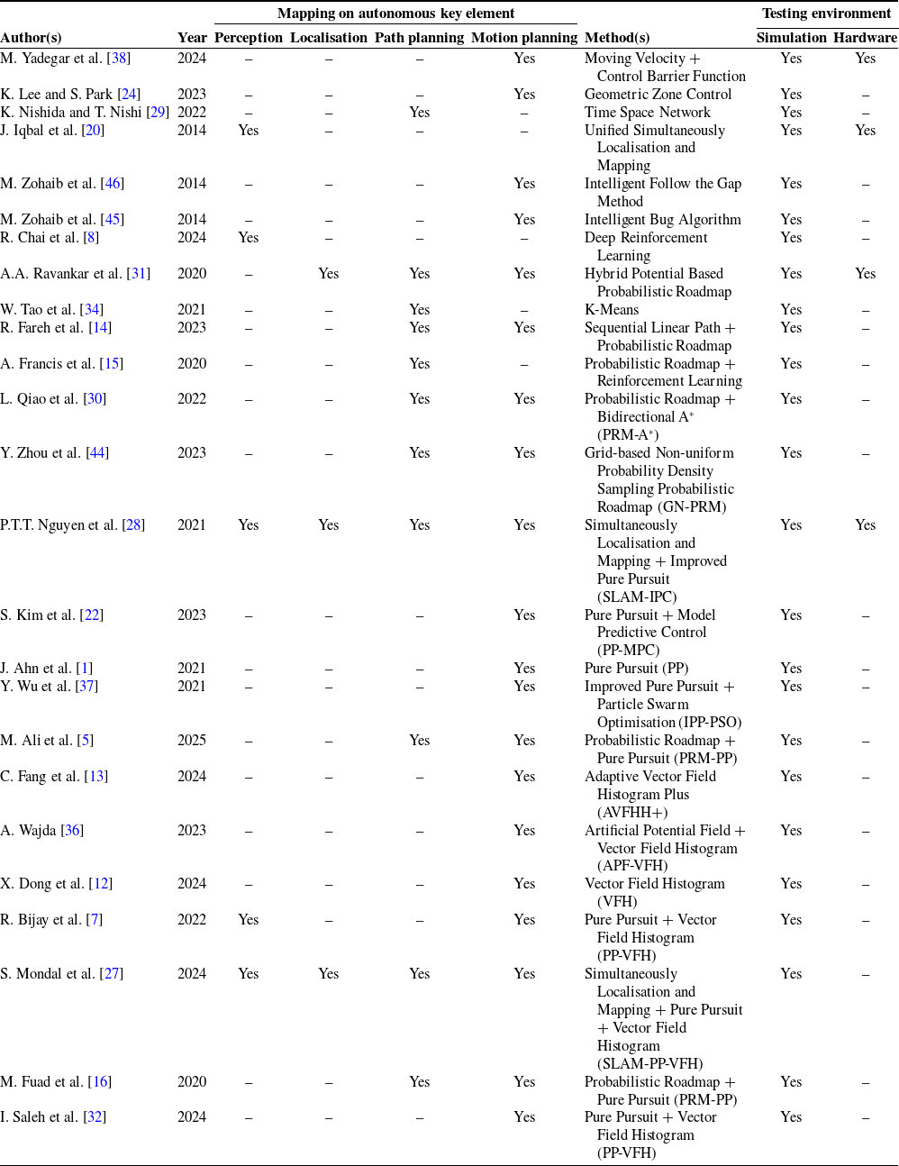
Table I summarises the technical publications on AGVs and mobile robots reviewed in this study, mapping each approach according to the four key elements of autonomous navigation: perception, localisation, path planning, and motion planning. As observed, most existing works are on path and motion planning elements which are confined to simulation-based testing, with limited validation on physical AGV platforms. To address this gap, the present study proposes a framework and strategy optimising PRM–PP–VFH implemented and tested on a real AGV platform.
Summary of related works on navigation elements and testing environments.

1.2. Research motivation, gap, and contributions
Conventional navigation system of AGVs continues to face challenges in obstacle avoidance. Despite significant progress, most existing studies treat path and motion planning algorithms such as PRM, PP, and VFH in isolation, with limited emphasis on integrated system validation using actual AGV platforms. The lack of a unified global–local planning framework that coordinates these modules and performs robustly under real industrial conditions remains a major research gap.
This study addresses these limitations by proposing and experimentally validating a proposed strategy on global–local motion planning that unifies global path planning, local trajectory tracking, and real-time obstacle avoidance within a single framework. Accordingly, this research is guided by the following research questions:
-
1. How PRM algorithm be optimised to generate the shortest and smoothest path with minimal waypoints generation?
-
2. How PP controller maintain accurate trajectory tracking without deviating from the global path?
-
3. To what extent VFH algorithm enhance obstacle avoidance and ensure safe navigation in real-world AGV operations?
The main contributions of this work are as follows:
-
1. Formulation of an integrated global–local motion planning framework enabling seamless coordination across multiple planning layers.
-
2. Detailed presentation of the fundamental and integration algorithmic design of PRM, PP, and VFH, providing a practical reference for developing autonomous navigation systems.
-
3. Experimental validation on a real AGV platform demonstrates a shortest path generation, path-tracking accuracy improved from 79.08% to 99.40% with lower percentage error. An effective collision avoidance under varying obstacle configurations with accuracy remained high at 99.10%.
2. Algorithms formulation
2.1. Probabilistic roadmap
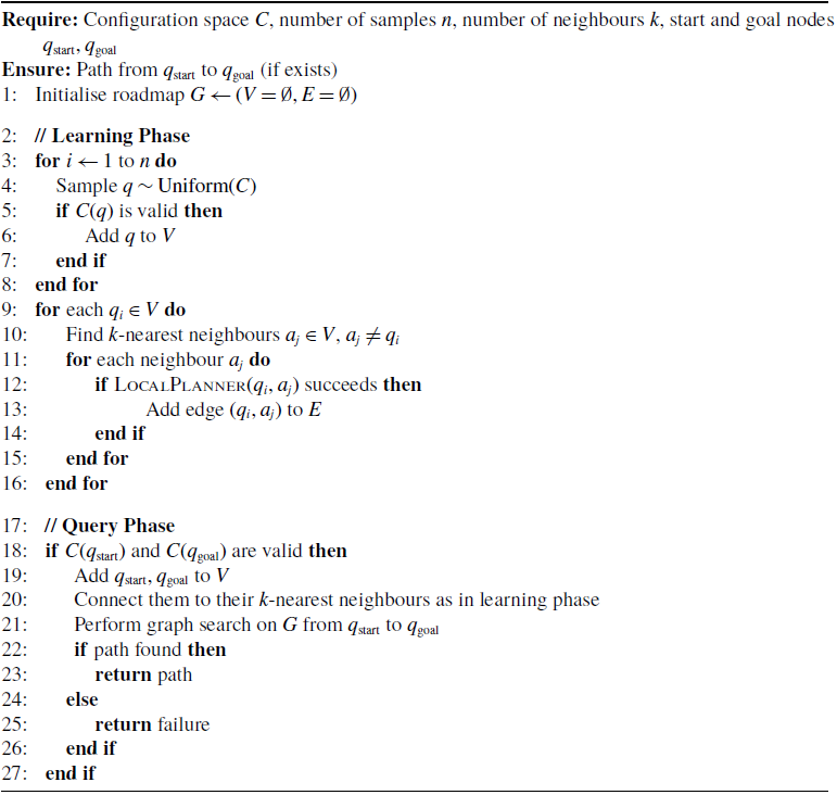
The PRM consists of two phases: learning and query. In the learning phase, there are two nodes: node sampling, which randomly samples points in the configuration space, and node connection, which connects nodes to edges if there is a collision-free path between them. The node sampling creates random samples (n) from the configuration space (C) in the map. Each sample node (q) represents the vehicle position or vehicle state. Collision checking will determine whether each
 $ q$
is in the free space (
 $ C_{\text{free}}$
). It will delete samples q that are in occupied space and are considered to be in a collision. Let
 $ q \in C$
be a random configuration, and C(q) be a collision-checking function as given by the equations
 \begin{equation} q \sim \text{Uniform}(C) \end{equation}
and
 \begin{align} C(q) = \begin{cases} \text{true} & \text{if } q \in C_{\text{free}} \\[3pt] \text{false} & \text{if } q \notin C_{\text{free}} \end{cases} \end{align}
The node connection will then find its k-nearest neighbours using a distance metric (d) for each sampled
 $ q$
as
 \begin{equation} d(q_i, q_j) = \sqrt {\sum _{k=1}^{n} \left ( q_{ik} - q_{jk} \right )^2} \end{equation}
and
 \begin{equation} \textit {LocalPlanner}(q_i, q_j) = \text{true} \end{equation}
The q was connected to its neighbours via a local planner. The planner determines if a straight path connecting two configurations is collision-free. For each pair of nodes (
 $ q_i$
,
 $ q_j$
), the connection is legitimate if the conditions in Eq. (2b) are met.
While in the query phase, two components are important, which are goal connection and path searching. The goal connection will connect the start location node (
 $ q_{\text{start}}$
) and the goal location node (
 $ q_{\text{goal}}$
) to the roadmap using the same k-nearest neighbours algorithm. The path searching will look for a path on the roadmap from
 $ q_{\text{start}}$
to
 $ q_{\text{goal}}$
by performing graph search techniques to identify the shortest path. Algorithm 1 shows the PRM pseudocode that demonstrates the flow of learning and the computation of the query phase.
2.2. Pure pursuit
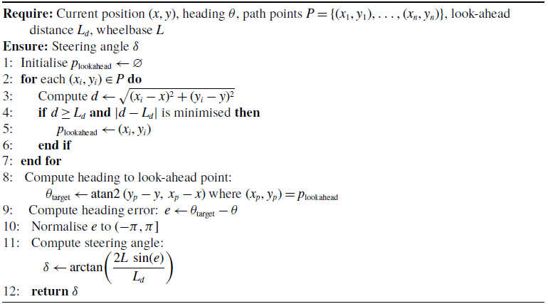
The PP calculates the vehicle steering commands required to follow a predetermined path by looking ahead at a preset distance and steering to that point as depicted in Figure 1. This approach requires two parameters to determine steering angle (
 $\tilde {\delta }$
), which are look-ahead point (
 $P$
) and steering angle (
 $\delta$
) calculations. Algorithm 2 shows the PP pseudocode.
Probabilistic roadmap (PRM)

Algorithm 1 Long description
An equation describing the probabilistic roadmap method for path planning. The algorithm starts with initialization of the roadmap G with empty sets for vertices V and edges E. The learning phase involves sampling n points uniformly from the configuration space C, adding valid points to V, and connecting each point to its k-nearest neighbors if a local planner succeeds. The query phase checks if the start and goal nodes are valid, adds them to V, connects them to their k-nearest neighbors, and performs a graph search to find the shortest path.
The difference between desired path and vehicle trajectory in the PP algorithm.

The PP detects the next point (
 $P_{i+1}$
) on the path at a look-ahead distance (
 $L_d$
) based on the vehicle’s current position (
 $X_t, Y_t$
) and heading (
 $\theta _t$
). The look-ahead point position (
 $X_p, Y_p$
) is calculated as
 \begin{equation} \sqrt {(x_p - x_t)^2 + (y_p - y_t)^2} = L_d \end{equation}
Pure pursuit (PP)

Algorithm 2 Long description
An algorithm for calculating the steering angle in pure pursuit path tracking. The algorithm initializes the look-ahead point and iterates through path points to find the point at the look-ahead distance. It then computes the heading to the look-ahead point, the heading error, and finally the steering angle using the arc tangent of the product of the wheelbase, sine of the heading error, and the reciprocal of the look-ahead distance.
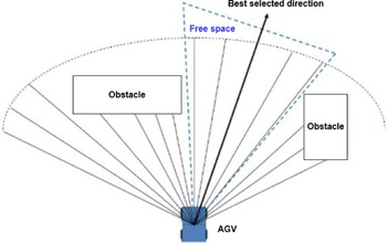
Best selected direction by the VFH algorithm performance based on LiDAR detection.

The steering angle (
 $\tilde {\delta }$
) formula is required for the vehicle to accurately follow a predefined path. It integrates several key parameters: the wheelbase of the vehicle (
 $L$
), the look-ahead distance (
 $L_d$
), and the error angle between the vehicle’s current heading and the direction towards a look-ahead point on the path as given by
 \begin{equation} \delta = \arctan \left (\frac {2L \sin\!(e)}{L_d}\right ) \end{equation}
where the e represents the difference between the vehicle’s current direction and the direction to the P, indicating how much the vehicle needs to turn to align with the desired path, while L represents the wheelbase as the distance between the front and rear axles of the vehicle, a fixed characteristic that influences how sharply the vehicle can turn.
2.3. Vector field histogram
The VFH creates a polar histogram of obstacle densities around the vehicle and chooses an appropriate steering direction (
 $\theta$
) to avoid obstacles and advance towards the goal as depicted in Figure 2. The vehicle must be equipped with sensors such as LiDAR or sonar to detect obstacles around it and populate a histogram grid. Each cell in the grid reflects the density of obstacles in a certain direction. It then turns the histogram grid into a polar histogram, with each bin representing the obstacle density in a specified angle direction relative to the vehicle.
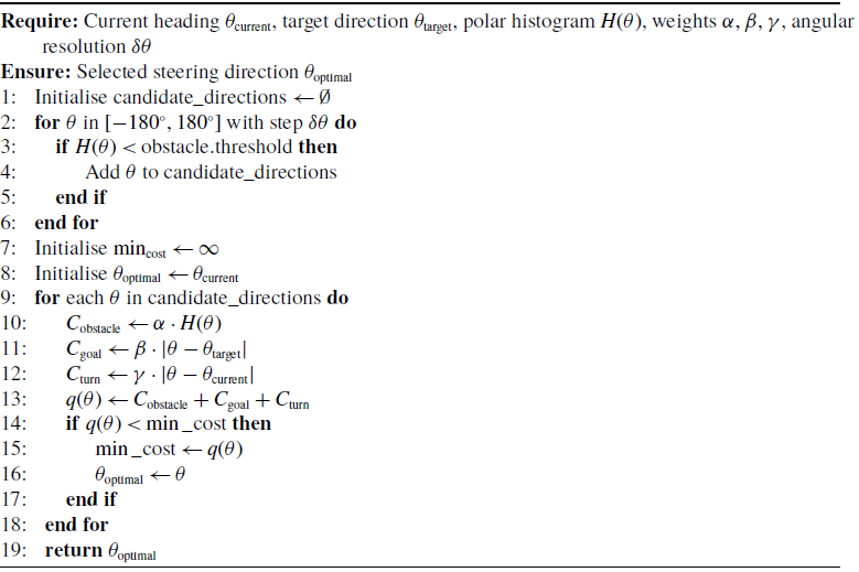
The VFH then identifies candidate directions with low obstacle densities that allow the vehicle to move forward. Each candidate way will be evaluated using a cost function that takes into account obstacle density (
 $\alpha$
), distance to destination (
 $\beta$
), and change in direction (
 $\gamma$
) expressed by
 \begin{equation} q(\theta ) = \alpha \cdot H(\theta ) + \beta \cdot D(\theta ) + \gamma \cdot \Delta \theta \end{equation}
where
 $ H(\theta )$
represents the histogram value at angle
 $ \theta$
, indicating the obstacle density in that direction. A higher
 $ H(\theta )$
suggests a higher likelihood of obstacles, which the vehicle should avoid. The coefficient
 $ \alpha$
weights this term, emphasising the importance of obstacle avoidance in the decision-making process. The
 $ D(\theta )$
is the target direction function, which measures how closely the direction
 $ \theta$
aligns with the desired target direction. A higher value of
 $ D(\theta )$
means the direction is closer to the target. The coefficient
 $ \beta$
weights this term, highlighting the priority of moving towards the goal. The
 $ \Delta \theta$
represents the change in direction from the vehicle’s current heading to the proposed direction
 $ \theta$
. This term accounts for the cost associated with turning. The coefficient
 $ \gamma$
weights this factor, penalising large changes in direction to promote smoother and more efficient paths.
Vector field histogram (VFH)

Algorithm 3 Long description
Panel A: The algorithm initializes candidate directions by iterating through angles from -180 to 180 degrees. It checks if the histogram value at each angle is below an obstacle threshold and adds valid angles to a list of candidate directions. Panel B: The algorithm then calculates costs for each candidate direction based on obstacle cost, goal cost, and turn cost. It selects the direction with the minimum total cost as the optimal steering direction.
By integrating these three factors, the function
 $ g(\theta )$
calculates a cost or score for each potential direction
 $ \theta$
. The objective is to minimise this cost, thereby identifying the optimal direction for the vehicle to move. Adjusting the weights
 $ \alpha$
,
 $ \beta$
, and
 $ \gamma$
allows the algorithm to balance the need to avoid obstacles, move towards the target, and minimise abrupt directional changes. The direction with the lowest
 $ g(\theta )$
value is selected as the best path for the vehicle, ensuring safe and efficient navigation in dynamic environments, and Algorithm 3 shows the VFH pseudocode. This approach enables the vehicle to make real-time decisions, constantly adjusting its path based on the current conditions and maintaining a balance between safety and efficiency.
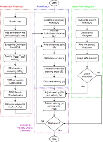
System workflow integrating PRM, PP, and VFH for the autonomous navigation framework.

3. Methodology
3.1. System model framework
Figure 3 illustrates a workflow showcasing the system model framework optimising the PRM, PP, and VFH algorithms to create a comprehensive navigation system for vehicle motion planning. It consists of two input parameters, namely LiDAR and odometry data, which are acquired by subscribing to the corresponding Robot Operating System (ROS) topics. Another one input is to specify which is the goal position, and another one output is to be published to the ROS topic, which is the velocity command to move the vehicle.
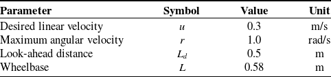
Pure pursuit (PP) algorithm parameter setting.

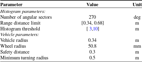
Vector field histogram (VFH) algorithm parameter setting.

Integrated PRM–PP–VFH navigation algorithm

Algorithm 4 Long description
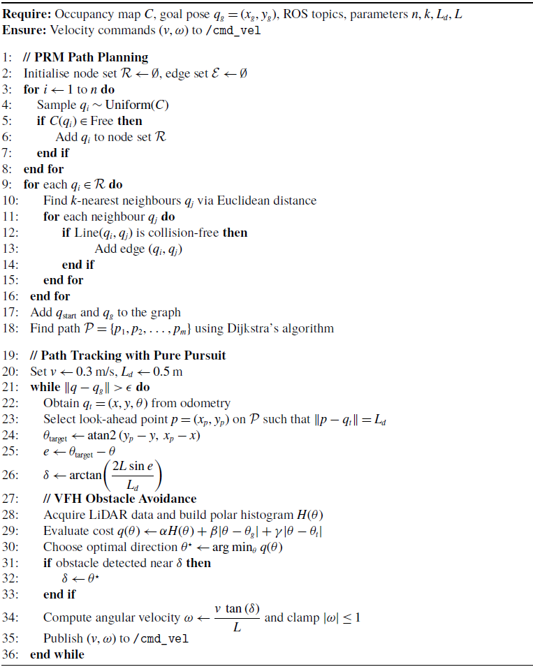
Panel A: PRM Path Planning. The algorithm initializes node and edge sets, samples points uniformly, and adds them to the node set if they are in free space. It then finds the k-nearest neighbors and adds edges if the line between them is collision-free. Finally, it adds the start and goal poses to the graph and finds the path using Dijkstra’s algorithm. Panel B: Path Tracking with Pure Pursuit. The algorithm sets initial velocity and look-ahead distance, then continuously obtains the current pose from odometry, selects a look-ahead point, and calculates the target angle and error. It then computes the angular velocity and publishes the velocity commands. Panel C: VFH Obstacle Avoidance. The algorithm acquires LiDAR data, builds a polar histogram, evaluates the cost function, chooses the optimal direction, and adjusts the angular velocity if an obstacle is detected.
The workflow begins with the PRM algorithm, where the environment map is uploaded into the model. A set of random points is sampled within this grid. The starting point (
 $X_t, Y_t$
) as the vehicle’s current pose is acquired from the ROS topic, which is odometry. The goal points are specified, and random points are sampled within the configuration space (
 $C$
) to form nodes (
 $q_n$
). These nodes are connected with local paths if they are collision-free, creating a graph structure. A shortest path search algorithm is then applied to find the optimal path from the start to the goal, resulting in a sequence of waypoints that guide the vehicle movement. These waypoints guide the vehicle movement through the environment.
Next, the PP algorithm takes over for path tracking, where it extracts the next goal point from the waypoints generated by PRM. The PP subscribes to odometry data from the ROS topic to acquire the vehicle’s current position (
 $X_t, Y_t$
) and orientation (
 $\theta _t$
). Then, the look-ahead distance (
 $L_d$
) is set, determining how far ahead the vehicle should look to find a look-ahead point (
 $P$
) along the path to compute steering commands. The necessary curvature to reach
 $P$
is calculated and converted into steering angles (
 $\delta$
) and velocities (
 $v$
), allowing the vehicle to adjust its steering and velocity to accurately follow the planned path. The PP algorithm parameters are listed in Table II. The desired linear velocity (
 $u$
) is set as constant in all carried-out experiments, which is at 0.3 m per second (m/s). The maximum angular velocity (
 $\omega$
) is capped at 1 rad/s (rad/s). The look-ahead distance (
 $L_d$
) is set at 0.5 m (m), which can be varied to change path tracking behaviour that is generated from waypoints set.
Simultaneously, the VFH algorithm ensures real-time obstacle avoidance by continuously subscribing to LiDAR data from the ROS topic to create a polar histogram representing obstacle densities around the vehicle. The algorithm identifies directions with low obstacle densities and selects the safest direction for movement. If an obstacle is detected in the current direction, the system recalculates a new safe direction, ensuring real-time obstacle avoidance. This continuous process allows the vehicle to navigate dynamically, avoiding collisions while following the planned path.
Table III lists the parameters for the VFH algorithm. Consists of two main parameters to be set, which are histogram and vehicle. In the histogram, the number of angular sectors is set to follow the LiDAR detection range, which is 270. Distance limits specify the distance range to consider for obstacle avoidance by specifying the limits in a two-element vector,
 $[lower, upper]$
. The lower limit is used to ignore sensor readings that intersect with parts of the vehicle, sensor inaccuracy at short distances, or sensor noise. The upper limit is the effective range of the sensor or is based on the application. Histogram threshold was used to compute binary histograms from the polar distance density. Any value higher than the upper threshold is considered occupied, which is “1,” whereas values smaller than the lower threshold are considered “0” or unoccupied. Values between the threshold limit are set to follow the previous binary histogram with the initial value of free space, “0.” This approach allows the vehicle to navigate dynamically, avoiding collisions while following.
Algorithm 4 shows the pseudocode for system model integrating these algorithms. The model is designed using MATLAB Simulink and communicates with vehicles equipped with ROS Noetic 20.04. The LiDAR is obtained from the ‘/front/scan‘ topic and is processed to extract range and angle information. Simultaneously, odometry data from the ‘/odometry/filtered‘ topic is converted from quaternion to Euler angles for use in navigation algorithms. The ‘/odometry/filtered‘ topic provides improved odometry by fusing raw odometry data from wheel encoders with measurements from the MicroStrain 3 DM-GX-5 IMU using sensor fusion techniques, which is the Extended Kalman Filter. While raw odometry is prone to cumulative errors due to factors like wheel slippage or uneven surfaces, the GX-5 IMU enhances accuracy by providing reliable inertial measurements of orientation and acceleration. This fusion reduces drift, improves pose and velocity estimation, and enhances vehicles’ localisation.
The decision-making layer is responsible for coordinating between global path tracking (PP) and local obstacle avoidance (VFH). The switching logic is governed by real-time LiDAR observations and heading alignment conditions. Specifically, the system operates in two modes: (i) path-following mode, where the PP controller tracks the reference trajectory generated by PRM, and (ii) obstacle-avoidance mode, where VFH is activated when obstacles are detected within a predefined safety distance along the current heading direction.
The switching condition is defined such that when the obstacle density in the forward sector exceeds a predefined threshold, control is temporarily transferred to the VFH module to compute a collision-free steering direction. Once the obstacle is cleared and the heading deviation relative to the reference path is within an acceptable tolerance, control is returned to the PP controller to resume trajectory tracking. This reactive switching mechanism ensures safe navigation while maintaining adherence to the global path. This switching logic is also reflected in Algorithm 4 (lines 30–33), where the steering command is adjusted based on obstacle detection conditions.
These algorithms work together by merging outputs from PP and VFH for a decision to generate smooth and safe motion commands. The final velocity (
 $v$
) commands, combining linear (
 $u$
) and angular velocities (
 $\omega$
), are published as geometry messages to the ‘/cmd_vel‘ topic, controlling the vehicle motion. The system model will deploy into a real vehicle to ensure efficient path planning, precise path tracking, and robust obstacle avoidance.
3.2. Experimental setup
It is important to note that all experiments in this study are conducted on a real physical AGV platform, rather than solely in simulation. The navigation framework is deployed in a real indoor environment, and all results reported in this work are obtained from actual system execution under practical operating conditions.
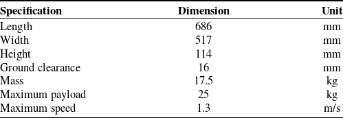
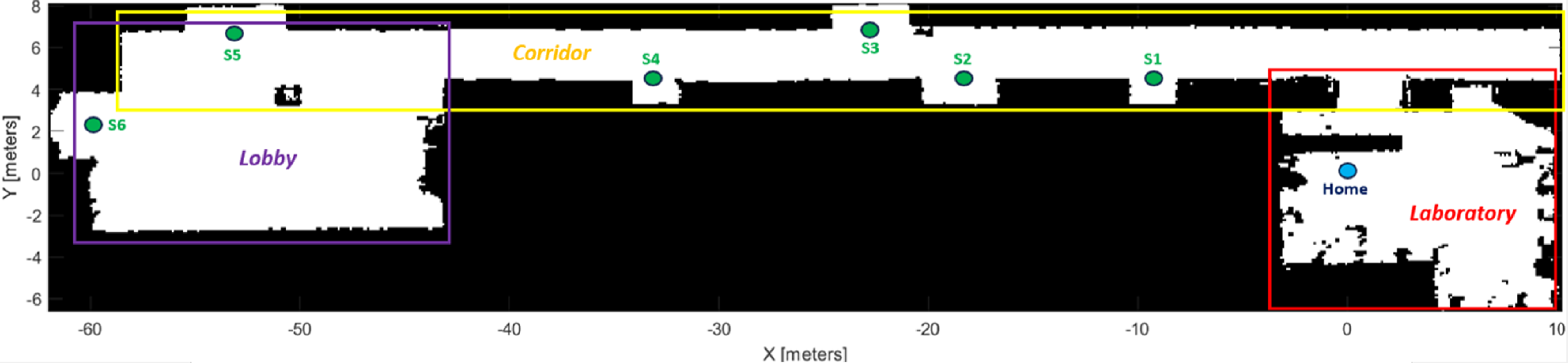
The experiment is being carried out in indoor environment which includes lobby, corridor and laboratory areas, as depicted in Figure 4, which is the map in occupancy grid map format. The size for the testing environment is 72.3 m (L) × 14.7 m (W). According to the system model workflow, mapping for environment testing must be done first. LiDAR and odometry are utilised in the mapping process to determine the position of vehicles using the Simultaneous Localisation and Mapping (SLAM) approach. During the mapping process, vehicles are manually moved via a console and Table IV lists the vehicle specifications. The vehicle is also equipped with internal sensors, which are LiDAR TIM551 2050001, MicroStrain IMU 3 DM-GX-5, and the encoder as wheel odometry.
Vehicle specifications.

Environment map in the occupancy grid map.

Figure 4. Long description
A diagram of an indoor environment map used for autonomous navigation. The map is divided into three main areas: Lobby, Corridor, and Laboratory. The Lobby is outlined in purple and contains a labeled point S6. The Corridor, outlined in yellow, extends horizontally and contains four labeled points: S1, S2, S3, and S4. The Laboratory, outlined in red, is located at the far right and contains a labeled point Home. The X-axis ranges from -60 to 10 meters, and the Y-axis ranges from -6 to 8 meters.
The occupancy grid map contains only two colours: black and white. The white colour represents the value ‘0’, which denotes an unoccupied space that can be reached by the vehicle. The black colour indicates the number ‘1’, which is an occupied space that the vehicle cannot reach due to the PRM not placing the node (q) in the already occupied space. The origin setting on the occupancy grid map must match the real position of the vehicle, which is considered to be homing at coordinate (0, 0). The occupancy grid map axis is known as the global axis, while the vehicle axis is known as the local axis. The goal station coordination points are as follows: Station 1 at (−10, 5.2), Station 2 at (−19.5, 5.2), Station 3 at (−23.5, 7.6), Station 4 at (−34, 5.2), Station 5 att (−54, 7.6), and Station 6 at (−60, 3.4). Every station serves as a checkpoint to access another laboratory and office space which are restricted from inclusion in this experiment.
The selection of key parameters for PRM, PP, and VFH was guided by both preliminary experimental evaluation and established practices in the literature. For the PRM algorithm, the number of nodes was systematically varied (100–1000 nodes) to identify an optimal trade-off between path smoothness, path length, and computational time.
For the PP controller, the look-ahead distance (
 $L_d$
= 0.5 m) was chosen based on the vehicle’s kinematic constraints and prior studies indicating that moderate look-ahead distances improve tracking stability while avoiding excessive oscillations [Reference Aizat, Kamarudin, Qistina, Han, Imran and Rahiman3]. Similarly, the VFH parameters, including histogram thresholds and distance limits, were determined based on LiDAR sensing range and vehicle safety constraints to ensure reliable obstacle detection while minimising false positives. These parameter selections ensure consistent and stable navigation performance across different environments.
Because the surrounding surface is just flat, the vehicle position must be accurate in two-dimensional (2D) axes, and this work will not count the z-axis. There was also no load put on or carried by the vehicle during the experiment that was carried out. The kinematic model designed for this system model is a differential drive approach as also presented in ref. [Reference Aizat, Kamarudin, Qistina, Han, Imran and Rahiman3] under robot kinematic section.
3.3. Experimental scenarios
The proposed system model is tested in three phases. The first phase is divided into two parts which demonstrated the path planning algorithm’s capability in simulation environment. The performance of the PRM algorithm was then evaluated with varying numbers of node parameters as a strategy to determine the optimal configuration from the vehicle’s home to Station 6 as the longest route. The goal was to identify the best number of nodes to be selected that offers the best path length, path smoothness, computational time and number of generated waypoints.
In the second part, the created PRM algorithm with the selected ideal number of nodes will be compared to algorithms often used in path planning studies, such as Rapidly Exploring Random Trees (RRT), A-Star (A*), and Dijkstra, with several criteria from the outcomes compared, including path length, path smoothness, number of generated waypoints, and computation time. Here is where the proposed strategy on path planning is highlighted.
The path length is calculated as the sum of Euclidean distances between consecutive waypoints along the path from starting to end point. For a path represented by
 \begin{equation} {P} = \{ {p}_1,\, {p}_2, \ldots, {p}_n \} \end{equation}
where
 $P_i$
is the node’s coordination as
 $(X_i, Y_i)$
and the formula is given by
 \begin{equation} L = \sum _{i=1}^{N-1} \sqrt {(x_{i+1} - x_i)^2 + (y_{i+1} - y_i)^2} \end{equation}
while path smoothness is calculated as the sum of absolute angular changes between consecutive segments of the path. For vectors, it is given by
 \begin{equation} \mathbf{v}_i = \mathbf{p}_{i+1} - \mathbf{p}_i \end{equation}
while angles are given by
 \begin{equation} \theta _i = \arctan \left (\frac {y_{i+1} - y_i}{x_{i+1} - x_i}\right ) \end{equation}
and the smoothness formula is given by
 \begin{equation} S = \sum _{i=1}^{N-2} \left | \theta _{i+1} - \theta _i \right | \end{equation}
The second phase of testing evaluates the PP algorithm’s path tracking capabilities with free obstacle space. When the PP algorithm acquires waypoints from PRM, it will begin manoeuvring the vehicle along the specified path. In this scenario, the vehicle’s odometry sensor plays a crucial role in ensuring that the vehicle is in the correct pose and heading towards its goal stations. As such, the objective of this test is to demonstrate the capabilities of fused odometry with IMU compared to standalone odometry. Figure 5 shows the real physical vehicle in the home station in the laboratory area.
Real physical AGV at home station in the laboratory environment.

The evaluation of the PP capability is based on the final positional distance error (
 $d_e$
), percentage error (%
 $E$
), and accuracy (
 $A$
) goal reaching. The
 $d_e$
is calculated using the Euclidean distance formula as given by
 \begin{equation} d_e = \sqrt {(X_2 - X_1)^2 + (Y_2 - Y_1)^2} \end{equation}
where the PRM’s last waypoint
 $(X_2, Y_2)$
is the reference value and the vehicle’s last stop position
 $(X_1, Y_1)$
is the actual value. The %
 $E$
is calculated as given by
 \begin{equation} \%E = \left (\frac {d_e}{d_r}\right ) \times 100 \end{equation}
where
 $d_r$
is the Euclidean distance of the reference position from the vehicle home at
 $(0,0)$
while the
 $A$
is calculated as given by
 \begin{equation} A = 100 - \%E \end{equation}
It should be noted that distance error and positional accuracy are computed using only the final stopping position of the AGV relative to the reference final waypoint. Therefore, these metrics represent final goal-reaching performance, not the accumulated tracking error over the full trajectory.
Then, the full set of collaborative algorithm proposed system model is test in the third phase. Obstacles such as construction cones will be located randomly. This time, the objective is to evaluate how effectively the VFH method performs when reaching obstacles that should not be present on the vehicle path computed by the PRM. Also, to assess the ability of the cooperation between the PP and VFH algorithms to make decisions to return to the original path after deviating due to obstacle avoidance. This time, the test only includes Station 1 as the shortest route and Station 6 as the longest route from the vehicle’s home.
To properly demonstrate the cooperative development of proposed system model, this test will be compared between vehicle trajectory generated in free space obtained in phase 2 (PRM-PP) and obstacle placement (PRM-PP-VFH).
4. Results and discussion
4.1. Evaluation of proposed strategy on global path planning
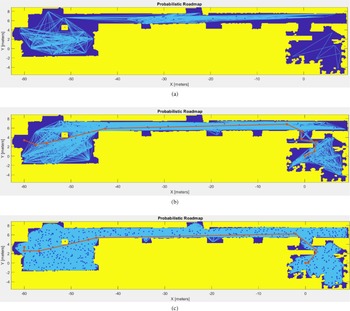
The proposed strategy was evaluated by varying the number of PRM nodes to determine the optimal configuration for the route from the home position to Station 6 (Figure 6). When the number of nodes was 50, the network was too sparse, resulting in disconnected waypoints. At 100 nodes, the path connected successfully but remained coarse, leading to less smooth trajectories. Increasing the nodes to above 200 improved waypoint continuity and smoothness, though excessive nodes significantly increased computational time.
Proposed strategy on global path planning performance at (a) 50 number of nodes; (b) 100 number of nodes; (c) 600 number of nodes.

Table V summarises the results for 100–1,000 nodes. The evaluation prioritised path smoothness, path length, computation time, and number of waypoints. Although 200 nodes produced the lowest smoothness value, the path length exceeded the average, making it less efficient. Configurations with 900–1,000 nodes achieved short paths but incurred excessive computation time. Among all, 600 nodes offered the best balance, yielding near-average smoothness and path length with moderate computation time and waypoint count. Therefore, 600 nodes were selected as the optimal configuration for subsequent testing. The inflated map parameter was minimally adjusted to maintain safety margins without compromising connectivity.
4.2. Comparison of path planning algorithm performance
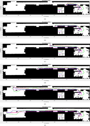
The PRM algorithm was evaluated with proposed 600 nodes and compared with RRT, A*, and Dijkstra to assess its path planning efficiency (Figure 7). The parameters for other algorithms were adapted from prior studies for fair benchmarking.
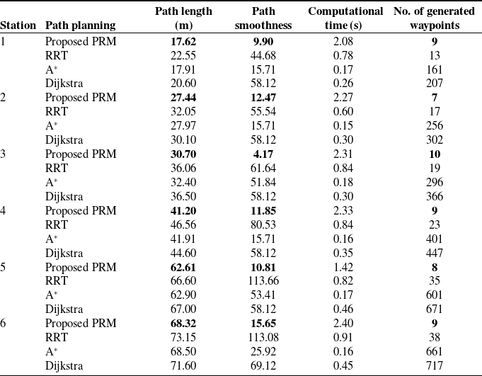
Table VI summarises the results across six goal stations. Evaluation priorities include path length, smoothness, number of waypoints, and computation time. The PRM consistently generated shorter and smoother paths than other algorithms, particularly in complex routes such as Stations 5 and 6. Although its computation time was slightly higher, the difference remained acceptable given its superior path quality.
Proposed strategy score on global path planning with different number of nodes.

Path generation from vehicle home to (a) Station 1; (b) Station 2; (c) Station 3; (d) Station 4; (e) Station 5; (f) Station 6.

Figure 7. Long description
Panel A: A line graph shows the path generation from the vehicle’s home to Station 1. The x-axis represents the X coordinate in meters, ranging from -60 to 0. The y-axis represents the Y coordinate in meters, ranging from -10 to 10. The graph includes multiple paths generated by different algorithms: PRM, RRT, A*, Dijkstra, with start and goal points marked. Panel B: A line graph shows the path generation from the vehicle’s home to Station 2. The axes and legends are the same as in Panel A. Panel C: A line graph shows the path generation from the vehicle’s home to Station 3. The axes and legends are the same as in Panel A. Panel D: A line graph shows the path generation from the vehicle’s home to Station 4. The axes and legends are the same as in Panel A. Panel E: A line graph shows the path generation from the vehicle’s home to Station 5. The axes and legends are the same as in Panel A. Panel F: A line graph shows the path generation from the vehicle’s home to Station 6. The axes and legends are the same as in Panel A.
Performance of proposed strategy compared to other path planning algorithms.

PRM also produced fewer waypoints, simplifying subsequent PP tracking and enhancing real-time feasibility. In contrast, A* and Dijkstra yielded dense waypoint sets that could burden onboard computation, while RRT often resulted in longer and less stable trajectories. Overall, PRM achieved the best balance between path efficiency, smoothness, and computational cost, validating its suitability for the proposed navigation framework.
It should be noted that the comparative analysis in this study focuses on widely adopted classical path planning algorithms (RRT, A*, and Dijkstra) to ensure a fair and consistent evaluation of global path generation performance. While advanced optimisation-based approaches such as model predictive control or safety corridor methods have demonstrated strong performance in dynamic environments, they typically require higher computational resources, system modelling, and parameter tuning. In contrast, the proposed framework emphasises a lightweight and modular integration of global planning, local tracking, and reactive obstacle avoidance, making it more suitable for real-time implementation in practical AGV systems.
PP algorithm performance between fused odometry and standalone odometry.

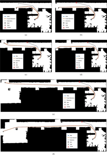
PP trajectory from vehicle home to (a) Station 1; (b) Station 2; (c) Station 3; (d) Station 4; (e) Station 5; (f) Station 6.

4.3. PP algorithm performance in free-path navigation
All results presented in this section are obtained from real-world experiments conducted using the physical AGV platform. The reported trajectories, positioning accuracy, and obstacle avoidance performance reflect actual system behaviour rather than simulation outputs.
The PP algorithm was evaluated using two odometry sources: fused odometry integrating the MicroStrain IMU and standalone odometry without fusion. Table VII presents the comparative results across six goal stations.
The fused odometry consistently achieved lower final distance error (
 $d_e$
) and higher final positioning accuracy (
 $A$
) than standalone odometry. Based on the six goal stations in Table VII, the average final distance error under fused odometry was 0.15, compared with 7.22 under standalone odometry. The corresponding average final percentage error was 0.61% for fused odometry and 20.92% for standalone odometry, while the average final positioning accuracy was 99.40% and 79.08%, respectively. These results indicate that the improvement is primarily attributable to the use of fused odometry, which enhances localisation quality and therefore supports more reliable PP-based path tracking.
Trajectory plots in Figure 8 further validate these findings. The fused-odometry trajectories closely follow the PRM path and reach goal stations with minimal deviation, whereas the standalone odometry paths show noticeable drift and occasional collisions, especially over longer routes.
Overall, the results demonstrate that sensor fusion markedly enhances the PP algorithm’s precision and stability by reducing drift, improving trajectory adherence, and ensuring reliable navigation performance in structured environments.
4.4. VFH algorithm performance in obstacle-path navigation
The complete system integrating PP and VFH was evaluated using PRM-generated global waypoints, as shown in Figure 9 and summarised in Table VIII. Obstacles were introduced to assess the system’s real-time avoidance capability.
Vehicle trajectory from vehicle home to (a) Station 1 and (b) Station 6.

PP with VFH performance for station 1 and station 6.

Results show that the integrated PP–VFH system maintained high accuracy while effectively avoiding obstacles. The average distance error (
 $d_e$
) was 0.15 units, nearly identical to free-space performance. The percentage error (%
 $E$
) increased slightly to 0.91%, and accuracy (
 $A$
%) remained high at 99.10%.
Trajectory analysis reveals that in obstacle-free conditions, the robot followed the PRM path precisely, while in obstructed scenarios, it successfully deviated around obstacles and rejoined the reference path with minimal deviation. These findings confirm that the integrated PP–VFH framework achieves reliable path tracking and robust obstacle avoidance with negligible performance loss.
In addition to static path quality metrics, the proposed framework demonstrates strong performance in complex environments through its real-time integration of PP and VFH. The system maintains stable navigation by continuously updating steering commands based on LiDAR feedback, enabling rapid response to unmapped or unexpected obstacles. The negligible increase in percentage error indicates that obstacle avoidance is achieved without compromising overall navigation accuracy.
Furthermore, the computational overhead introduced by the VFH module remains low due to its efficient histogram-based processing, allowing real-time execution within the system constraints. Compared to classical planners such as RRT and A*, which primarily focus on global path generation, the proposed integrated framework provides a more comprehensive solution by combining global planning, local control, and reactive obstacle avoidance within a unified architecture.
The effectiveness of the proposed framework lies in its ability to maintain a balance between global path optimality, local tracking accuracy, and real-time obstacle avoidance. Unlike methods that focus solely on path planning or control, the integrated approach ensures consistent performance across different navigation stages. The results demonstrate that the system can adapt to environmental changes while preserving high positioning accuracy, highlighting its suitability for practical deployment in structured industrial environments.
5. Conclusion and future work
This study proposed a comprehensive global–local motion planning strategy for AGVs collision-free by optimising the PRM, PP, and VFH algorithms in a single framework. The experimental findings confirmed that the proposed approach effectively addresses the three key research questions outlined in this work.
First, the varies of PRM number of nodes was optimised to generate the shortest and smoothest path with minimal waypoint generation, balancing path efficiency and computational cost as the first strategy. Second, the PP controller successfully maintained accurate trajectory tracking without deviating from the global path, achieving minimal distance and percentage errors through fused odometry integration as second strategy. Third, the VFH algorithm enhanced obstacle avoidance performance with decision-making layer for switching, ensuring safe, smooth navigation, and capable back to desired path as the last strategy.
Overall, the proposed framework demonstrated robust and adaptive autonomous navigation in both simulation and real-world indoor environments. The framework will serve as a reference and guide for engineers or researchers who wish to migrate from a conventional AGV navigation system to autonomous. Unlike many existing studies that rely solely on simulation, this work demonstrates real-world validation on a physical AGV platform, enhancing the practical relevance of the proposed framework.
Although the experimental validation is conducted in structured indoor environments, dynamic obstacles are introduced during testing to evaluate the real-time responsiveness of the proposed framework. The integration of LiDAR-based sensing and the VFH algorithm enables the system to react to unexpected obstacles and rejoin the reference path with minimal deviation.
However, it is acknowledged that the current study does not explicitly consider highly unstructured or large-scale open environments, such as unloading areas with complex and unpredictable obstacle behaviour. Extending the proposed framework to such scenarios remains an important direction for future work.
Future work will focus on extending the system’s capabilities to dynamic obstacle scenarios, incorporating machine learning for adaptive decision-making, and validating performance in industrial-scale deployments integrated with fleet management and scheduling systems.
Author contributions
Muhammad Aizat conceived the study, developed the algorithms, conducted the experiments, and wrote the manuscript. Chia Siang Kok and Mohd Zulkifli supervised on the experimental hardware setup. Jamshed Iqbal reviewed the manuscript and provided valuable comments to improve the quality of the work. Wan Rahiman supervised the research, guided the overall methodology, and contributed to the final revision of the manuscript. All authors have read and approved the final version of the manuscript.
Financial support
This work was supported by the Universiti Sains Malaysia through External Grant Industry (BJIM) under grant number A305-LR-AKH001-0044020512-W116. The work of Muhammad Aizat Abu Bakar was funded by the Malaysian Ministry of Higher Education (MoHE) and Universiti Malaysia Perlis (UniMAP) under the Bumiputera Academic Training Scheme Scholarship.
Competing interests
The authors declare no conflicts of interest exist.
Ethical approval
Not applicable.
Use of AI
The author acknowledges the use of AI tools, including ChatGPT 5.0 and QuillBot, during the preparation of this manuscript. These tools were used solely for language refinement, grammar improvement, and technical formatting, such as generating LaTeX code for algorithms, figures, and tables. All content was thoroughly reviewed and verified by the author, who takes full responsibility for the accuracy and integrity of the final version of the paper.