





1. Introduction
It is a universally acknowledged fact that the macroscopic description of a contact line can take one of two forms (Dussan V. & Chow Reference Dussan, E. and Chow1983; Bonn et al. Reference Bonn, Eggers, Indekeu, Meunier and Rolley2009; Wilson & D’Ambrosio Reference Wilson and D’Ambrosio2023). The contact line may either be mobile, or stuck at a fixed position (the pinned case), as illustrated in figure 1. For example, in describing drop evaporation (Stauber et al. Reference Stauber, Wilson, Duffy and Sefiane2014; Wilson & D’Ambrosio Reference Wilson and D’Ambrosio2023), the pinned case is often referred to as the ‘constant radius’ or (CR) mode, whereas the mobile case is the ‘constant angle’ or (CA) mode. If the contact line position can be moved infinitesimally without incurring any work (figure 1
a), then the energy balance yields the equilibrium angle
 $\theta _{{eq}}$
(also known as Young’s angle) (de Gennes Reference de Gennes1985): i.e.
 \begin{equation} \gamma \cos \theta _{eq} = \gamma _{SV} - \gamma _{SL}. \end{equation}
Here
 $\gamma$
is the energy per unit area of liquid–vapour interface, while
 $\gamma _{SV}$
and
 $\gamma _{SL}$
are the corresponding energies for the solid–vapour and solid–liquid interfaces, respectively.
In the pinned case, which may arise from random disorder on the surface (Bonn et al. Reference Bonn, Eggers, Indekeu, Meunier and Rolley2009), or from patterning of the surface (Quéré et al. Reference Quéré, Lafuma and Bico2003), the contact line is stuck at a topographical or chemical barrier. A possible pinning configuration is illustrated in figure 1(b). Since the contact line is stuck on the tip of an asperity of vanishing size (Hong, Fontelos & Hwang Reference Hong, Fontelos and Hwang2016; Graña-Otero & Parra Fabián Reference Graña-Otero and Parra Fabián2019), all orientations of the interface are energetically equivalent, and the contact angle is not fixed by a local condition. Instead, as we will see, the contact angle
 $\theta$
is fixed entirely by the dynamics of the liquid adjacent to it.
Two different states of a contact line. (a) The contact line is allowed to move without energy barrier. Since there should be no work associated with a virtual displacement in equilibrium, the equilibrium contact angle is Young’s angle (1.1). (b) The contact line is stuck on an asperity. All possible angles
 $\theta$
are energetically equivalent.

Although a huge amount of literature treats the dynamics of thin films bounded by a mobile contact line, the second case of a pinned contact line is often examined only with regard to the conditions under which depinning occurs, i.e. when the contact starts to move again. This happens, for example, when a drop is placed on an incline that is is sufficiently steep (Dussan V. & Chow Reference Dussan, E. and Chow1983). An exception to this rule is a recent numerical study of an oscillating drop with a pinned contact line, in a regime dominated by inertia (Sakakeeny & Ling Reference Sakakeeny and Ling2021). Here, we inquire about the nonlinear dynamics of a viscous fluid film while the contact line position remains fixed. Related thin film problems with fixed boundaries have been considered by Bernis, Hulshof & King (Reference Bernis, Hulshof and King2000) and Bowen & King (Reference Bowen and King2001). For example, one can imagine placing a drop on a rough substrate, such that the contact line is always pinned. In general, the initial shape will not be an equilibrium shape, and the drop shape evolves until a steady state, corresponding to thermodynamic equilibrium, is reached.
We assume that transversal variations of the contact line position (e.g. contact line roughness (Bonn et al. Reference Bonn, Eggers, Indekeu, Meunier and Rolley2009), are negligible. This could also be ensured by pinning the contact line to a specially prepared straight and sharp-edged ridge. Moreover, we assume that vertical scales of the film are small compared with horizontal scales, so that the lubrication or thin-film approximation is valid. Within this framework, we show that the contact angle is determined self-consistently through a coupling to the film profile
 $h(x,t)$
away from the contact line.
We assume that all lengths and time have been made dimensionless, for example, using the width of the fluid film and the capillary speed
 $\gamma /\eta$
, where
 $\gamma$
is the surface tension coefficient and
 $\eta$
is the viscosity. Then the Laplace pressure condition at the interface requires that
 $p = -h_{xx}$
is the pressure inside the fluid film. As the flow is driven by pressure gradients
 $p_x$
, the fluid flux is
 $f = h^n p_x$
, where
 $h^n$
is known as the mobility. The mobility measures the viscous resistance to the flow, which depends on the geometry and other physical effects present. Finally, by applying mass conservation
 $h_t + f_x = 0$
, we arrive at the thin film equation
 \begin{equation} h_t + (h^n h_{xxx})_x = 0, \quad n\gt 0, \end{equation}
which has been used very successfully to describe the evolution of thin layers of viscous fluid (Oron, Davis & Bankoff Reference Oron, Davis and Bankoff1997; Bonn et al. Reference Bonn, Eggers, Indekeu, Meunier and Rolley2009).
The case
 $n=3$
describes a layer of viscous fluid on a solid substrate, subject to the no-slip boundary condition. As will be discussed in more detail in the final section, for
 $n=3$
(1.2) is unable to describe contact line motion (Huh & Scriven Reference Huh and Scriven1971; Zhao Reference Zhao2014). To address this problem, various slip laws (Kulkarni, Fullana & Zaleski Reference Kulkarni, Fullana and Zaleski2023) have been introduced, the simplest of which is the Navier boundary condition (Bonn et al. Reference Bonn, Eggers, Indekeu, Meunier and Rolley2009). For Navier slip with slip length
 $\lambda$
,
 $h^n$
in (1.2) is replaced by
 $h^3 + \lambda h^2$
, which for small
 $h$
, is dominated by the second, slip term. As a result, the first term
 $h^3$
is often dropped, so that effectively
 $n=2$
, as long as one is describing the neighbourhood of the contact line, or the slip length is exceptionally large. In using (1.2) throughout, we adopt this logic, and also treat
 $n$
as a continuous variable, to represent slip of varying effectiveness.
A summary of the problems considered in this paper. (a) At some initial time
 $t=0$
, an initial drop shape is prescribed (here assumed symmetrical), and the drop is pinned between two sites. (b) At early times
 $t\ll 1$
, the dynamics is local if
 $n\ne 3$
. If
 $n=3$
, the dynamics of the contact line is driven from regions far away from the contact line. (c) Finally, for long times, the contact angle, and the entire drop relaxes toward a quadratic equilibrium shape.

For the rest of this paper, we assume that the contact line is fixed at
 $x=0$
, while the fluid occupies some region
 $x\gt 0$
. For small slopes, the contact angle is then given by
 $\theta (t) = h_x(0,t)$
. For simplicity, we treat the representative problem of a two-dimensional drop or strip of fluid of finite width. Starting from a smooth but otherwise arbitrary initial condition, we investigate the dynamics of a drop that eventually relaxes toward an equilibrium profile, which is quadratic in the thin film approximation. In the next section, we derive the evolution equation for
 $\theta (t)$
, which is coupled to the dynamics of the fluid film. We then describe a numerical method, based on (1.2), to describe the dynamics of the free surface of the drop, from early times until equilibrium is reached.
In § 3, we demonstrate that the early-time dynamics of the contact angle can, in fact, be described by a linearised evolution equation. This insight is used to find a local similarity solution describing the contact angle for early times, assuming
 $n\ne 3$
. The degenerate, but physically most relevant case,
 $n = 3$
, is treated in § 4. The solution now consists of several regions, which are treated separately and subsequently matched together. Section 5 describes relaxation of the drop toward equilibrium. A pictorial overview of the cases considered is shown in figure 2. We close with a discussion, paying particular attention to the relevance of our results to Huh and Scriven’s contact line paradox (Huh & Scriven Reference Huh and Scriven1971). Some details of calculations are found in an Appendix.
2. Dynamics of the contact line and numerical method
We consider the evolution of a profile
 $h(x,t)$
, as described by (1.2), which, for simplicity, we assume is symmetrical. The edges of this ‘drop’ are pinned at
 $x=0$
and
 $x=2$
, respectively (and after appropriate scaling). Since (1.2) is of fourth order in space, four boundary conditions are needed. At the contact line, we expect the flux to vanish (Bernis et al. Reference Bernis, Hulshof and King2000), so the boundary conditions are
 \begin{equation} h(0,t) = 0, \quad \left .h^n h_{xxx}\right |_{x=0} = 0, \end{equation}
while, at the point of symmetry,
 $h_x(1,t) = h_{xxx}(1,t) = 0$
. If the drop is not symmetrical, the analogue of (2.1) is imposed at the other contact line. For convenience, we write
 $n = 3-\delta$
, so that
 $\delta = 0$
refers to the critical case
 $n=3$
. To find the evolution equation for
 $\theta$
, we have to find the term that balances the first term in
 $h_t(x,t) = \dot {\theta } x + O(x^2)$
. This leads to the expansion (Bernis et al. Reference Bernis, Hulshof and King2000)
 \begin{equation} h = \theta x + bx^2\ln x + c x^2,\; \delta = 0; \quad h = \theta x + \frac {b}{\delta }x^{2+\delta } + \left (c - \frac {b}{\delta }\right )x^2,\; \delta \ne 0; \end{equation}
up to terms of higher order. The representation (2.2) is used later in the numerical description of the contact line. We have written the case
 $\delta \ne 0$
such that the case
 $\delta = 0$
emerges in the limit. Inserting (2.2) into (1.2) and comparing terms of order
 $x$
, we obtain the dynamical equation
 \begin{equation} \dot {\theta } = -2(2+\delta )(1+\delta ) \theta ^{3-\delta } b \end{equation}
in both cases; (2.3) simplifies to
 $\dot {\theta } = -4\theta ^3 b$
for the critical case
 $\delta =0$
. This introduces a nonlinear coupling between the contact angle and the shape of the drop, closing the system of equations to be solved. Curiously, we are not aware of (2.3) having been written down before.
In the limit of long times, we expect the drop to converge toward the equilibrium profile
 \begin{equation} h_{eq} = \frac {3V}{4} x(2-x), \end{equation}
fixed uniquely by the drop volume
 $V$
and the drop being confined between
 $0$
and
 $2$
.
2.1. Numerics
Our numerical scheme follows others used previously to solve the highly nonlinear thin film equation (Dupont et al. Reference Dupont, Goldstein, Kadanoff and Zhou1993; Eggers & Fontelos Reference Eggers and Fontelos2015): we use a fully implicit finite difference scheme with a staggered grid. To that end, (1.2) is split as
 \begin{equation} h_t + (h^{n-1} f)_x = 0, \quad f = h h_{xxx}, \end{equation}
and the interval
 $[0,1]$
is divided into grid points
 $x_i, i=1\dots k$
, with
 $x_1 = 0$
and
 $x_k = 1$
;
 $f_i, i=1\dots k-1$
is defined at the midpoints. The profile
 $h_i$
is used to compute
 $p_k = h_{xx}$
at the grid points. At the right-hand end, we impose symmetry of
 $h$
, and antisymmetry of
 $f$
. The values
 $f_i$
are calculated from
 $p_i$
using centred differences, where
 $p_i$
is calculated with a 5-point scheme, valid for arbitrary grid spacings. The values of
 $f$
and
 $f_x$
, needed at the grid points for the first equation, are also calculated with second-order accuracy.
Near the contact line, we impose the expansion (2.2), where the contact angle
 $\theta$
is a separate variable (which takes the place of
 $f_1$
), and which evolves according to (2.3). The value of
 $f_1$
, between
 $x_1$
and
 $x_2$
, is calculated from (2.2). Likewise, for a given
 $\theta$
, the coefficients
 $b$
and
 $c$
are found from equating (2.2) to
 $h_{2}$
and
 $h_{3}$
at
 $x_{2}$
and
 $x_{3}$
, respectively. Then, if we let
 $\varDelta = x_2$
, and
 $x_3 = 2\varDelta$
, we find that
 \begin{equation} b = \frac {1}{\varDelta \ln 2}\left (\frac {\theta }{2} - \frac {h_3-4h_2}{4\varDelta }\right ), \quad c = -b\ln \varDelta + \frac {1}{\varDelta }\left (\frac {h_2}{\varDelta }-\theta \right ). \end{equation}
In summary, the variables are
 $h_2, \dots , h_{k-1}$
,
 $f_2, \dots , f_{k-1}$
and
 $\theta$
: a total of
 $2k-4+1 = 2k-3$
. The equations are the first of (2.5), evaluated at
 $x_2, \dots , x_{k-1}$
, and the second of (2.5), evaluated at
 $x_{1/2}, \dots , x_{k-1/2}$
, with the extra equation (2.3).
The change in contact angle
 $\dot {\theta }$
as a function of time from a numerical solution of (1.2) with
 $n=3$
and initial condition
 $h_0(x) = \bar {h}\sin (\pi x/2)$
,
 $\bar {h} = 0.1$
. Thus
 $V = 4\bar {h}/\pi$
. For long times,
 $\dot {\theta }$
decays such as
 ${\rm{e}}^{-0.57 t}$
to zero (see § 5); this exponential decay is shown as the dashed line. For short times, on the other hand,
 $\theta$
appears to remain constant for some time (
 $\dot {\theta } = 0$
); we show that, instead,
 $\dot {\theta }$
behaves according to
 $\displaystyle {\rm{e}}^{-3/(2t^{1/3})}$
.

We use a strongly graded grid, with the smallest (constant) grid spacing near
 $x=0$
, and which is slowly increased away from
 $x=0$
, until a maximum spacing of
 $10^{-3}$
is reached. Our numerical scheme is fully implicit, and second order in time, using a step-halving method. Comparison between the two steps serves to adjust the time step, in order to maintain sufficient temporal resolution.
3. Early-time dynamics
We begin looking at very early times after the drop has been set down. Although the original equations (1.2) and (2.3) are highly nonlinear, for very early times the equations are effectively linear, as we now show. We proceed in several steps.
3.1. Effective linear dynamics
We assume that the initial condition can be expanded into a power series of the form
 \begin{equation} h_0 = a_0 x + b_0 x^2 + c_0 x^3 + O(x^4). \end{equation}
Since
 $x$
is small close to the contact line, we can view
 $c_0 x^3$
as a small perturbation to the equilibrium profile
 $h_{eq} = a_0x + b_0 x^2$
, around which we linearise by writing
 $h(x,t) = h_{eq}(x) + \delta h(x,t)$
. We thus consider the linear equation
 \begin{equation} \delta h_t + \left (h_{eq}^n\delta h_{xxx}\right )_x = 0, \end{equation}
so we have confirmed numerically that the early time behaviour of (3.2) is indeed the same as that of the full equation.
The change in contact angle
 $\dot {\theta }(t)$
as function of time. Solid line: solution of (1.2) with
 $n = 3$
and initial condition
 $h_0(x) = x(2 - x) + 0.1 x^2(2-x)^2$
; contact angle found from (2.3). Boundary conditions are
 $h(0,t) = 0$
and
 $h_x(1,t) = h_{xxx}(1,t) = 0$
. Long-dashed line: solution of the linearised leading-order equation (3.2) with
 $h_{eq} = 2x$
and initial condition
 $\delta h(x,0)= 0.1 x^2(2-x)^2$
. Boundary conditions for the linearised problem are
 $\delta h(0,t) = 0$
and
 $\delta h(1,t) = \delta h(1,0), \delta h_{xx}(1,t) = \delta h_{xx}(1,0)$
. Dot-dashed line: equation (3.2) with
 $h_{eq} = 2x$
and initial condition
 $\delta h(x,0) = -0.4 x^3$
, with boundary conditions
 $\delta h(0,t) = 0$
and
 $\delta h(1,t) = -0.4, \delta h_{xx}(1,t) = 2.4$
. (a) All three curves; (b) a detail of the dashed and dot-dashed lines, with the amplitude of the latter adjusted.

In a second step, we argue that, close to the contact line,
 $h_{eq}^n$
is dominated by the linear term
 $h_{eq} \approx a_0 x$
; hence, we obtain
 \begin{align} \delta h_t + \left (a_0^nx^n\delta h_{xxx}\right )_{x} = 0, \end{align}
which is a linear and homogeneous problem. Since
 $a_0 x + \delta h(x,t)$
is no longer the profile of a droplet, we can no longer impose the same symmetry conditions. Instead, we argue that, as far as representing the far-field conditions are concerned, we can impose that the thickness and curvature of the drop profile changes little when imposed on the scale of the drop radius (which is normalised to unity), and viewed over the short time scale on which the contact line region is evolving. We thus impose
 \begin{equation} \delta h(1,t) = \delta h(1,0), \quad \delta h_{xx}(1,t) = \delta h_{xx}(1,0) . \end{equation}
This idea is tested in figure 4 for the critical case
 $n = 3$
. In figure 4(a), using the solid line, we show a simulation of the fully nonlinear equation (1.2) with contact angle condition (2.3) and boundary conditions
 $h(0,t) = 0$
,
 $h_x(1,t) = h_{xxx}(1,t) = 0$
; for the initial profile, we take
 $h_0(x) = x(2 - x) + 0.1 x^2(2-x)^2$
, where
 $h_{eq}(x) = x(2-x)$
is the equilibrium profile, and
 $\delta h(x,0) = 0.1 x^2(2-x)^2$
the initial perturbation. This solution is compared with the linearised equation (3.2), in which we have also replaced
 $h_{eq}(x)$
by the leading order expansion
 $h_{eq} = 2x$
of the initial condition. As the initial condition of the linearised problem, we once more take
 $\delta h(x,0) = 0.1 x^2(2-x)^2$
and apply the boundary conditions (3.4).
The linearised form of the evolution equation for the contact angle (2.3) is
 \begin{equation} \dot {\theta } = -2(2+\delta )(1+\delta )b, \end{equation}
with
 $b$
once more defined by (2.2), but with
 $\theta$
now representing the deviation of the contact angle from its initial value. The resulting solution for
 $\dot {\theta }$
is seen in figure 4(a) to agree very well with the full nonlinear solution, at least for
 $t \lesssim 3\times 10^{-5}$
. In a third step, we further approximate the initial condition of the linearised problem as
 $\delta h(x,0) = -0.4 x^3$
, derived from the cubic term of
 $\delta h(x,0) = 0.1 x^2(2-x)^2$
. The boundary conditions are once more given by (3.4).
The resulting solution
 $\dot {\theta }$
is now shown as the dot-dashed line in figure 4(a). To appreciate the agreement with the dashed line, which includes higher-order terms in the initial condition, we show a zoomed-in version of the same curves in figure 4(b). The agreement for earlier times is such that the two curves can almost not be distinguished; however, we have allowed for a small change in amplitude of the dot-dashed line to reach optimal agreement. This is natural, since we are solving a linear equation, and the effective driving amplitude will have changed slightly on account of the higher order terms.
In summary, up to an overall constant, and after appropriate rescaling, we may describe the short-time dynamics of the full non linear contact line problem by
 \begin{equation} \delta h_t + \left (x^n\delta h_{xxx}\right )_{x} = 0, \end{equation}
with initial condition
 $\delta h = x^3$
. The boundary conditions are
 \begin{equation} \delta h(0,t) = 0, \quad \delta h_x(0,t) = \theta , \quad \quad \delta h(1,t) = 1, \quad \delta h_{xx}(1,t) = 6, \end{equation}
where the dynamics of
 $\theta$
is given by (3.5). To remove unnecessary constants, in our analysis of (3.6) we found it useful to take the second derivative of (3.6), to obtain an equation for the curvature
 $\kappa = \delta h_{xx}$
of the perturbation
 \begin{equation} \kappa _t + \left (x^{3-\delta } \kappa _x\right )_{xxx} = 0, \end{equation}
with initial condition
 $\kappa = 6 x$
. From (2.2), we find that, for small
 $x$
,
 \begin{equation} \kappa = \frac {(2+\delta )(1+\delta )b}{\delta } x^{\delta } + 2\left (c - \frac {b}{\delta }\right ),\; \delta \ne 0,\quad \kappa = 2 b \ln x + 3b + 2c,\; \delta = 0. \end{equation}
Inserting the initial condition into (3.8), we obtain
 $\kappa _t = -6(3+\delta )(2+\delta )(1+\delta )x^{\delta }$
, so that at short times the solution is
 \begin{align} \kappa = 6x - 6(3+\delta )(2+\delta )(1+\delta )x^{\delta } t. \end{align}
This means that new terms of the form (3.9) are generated immediately, and the contact angle must change. We can expect a local solution driven by the dynamics of the contact line alone. If, on the other hand,
 $\delta = 0$
,
 $\kappa = 6x - 36 t$
solves (3.8) exactly and is compatible with the initial conditions. The dynamics is now driven by the fact that the solution is no longer compatible with the boundary condition at the other end: a non-local process. As a result, the contact angle hardly changes initially, since the driving is extremely weak. We start with the local generic, case
 $\delta \ne 0$
.
3.2.
The contact angle,
 $\delta \ne 0$

We begin with the case where
 $n$
does not equal the generic value for a liquid film on a solid substrate. We are looking for similarity solutions of the form
 $\kappa = t^{\gamma } P(\xi )$
(Bernis et al. Reference Bernis, Hulshof and King2000), where
 $\xi = x/t^{1/(1+\delta )}$
, so that (3.8) is satisfied. For large
 $\xi$
, this solution has to match
 $\kappa = 6x$
; this implies that
 $\gamma = 1/(1+\delta )$
, so that
 \begin{equation} \kappa = t^{1/(1+\delta )} P(\xi ), \quad \xi = x/t^{1/(1+\delta )} \end{equation}
is the form of the similarity solution, with
 $P(\xi ) = 6\xi$
for large arguments. The similarity equation becomes
 \begin{equation} \frac {P - \xi P_{\xi }}{1+\delta } + \left (\xi ^{3-\delta } P_{\xi }\right )_{\xi \xi \xi } = 0. \end{equation}
Four linearly independent solutions
 $P_1,P_2,P_3$
and
 $P_4$
to (3.12) can be found in terms of generalised hypergeometric functions (Olver et al. Reference Olver, Lozier, Boisvert and Clark2010), as given in Appendix A, cf. (A1)–(A4); they are real for
 $\xi \gt 0$
. Very similar solutions to an elastic fourth-order problem have been described in (Stone & Duprat Reference Stone and Duprat2016). The solutions
 $P_2$
and
 $P_4$
are singular at the origin, and on account of (3.9) have to be excluded. The remaining solutions
 $P_1$
and
 $P_3$
grow exponentially at infinity, while we demand
 $P(\xi ) = 6\xi$
. As shown in detail in Appendix A, we can cancel the exponential growth by superimposing
 $P_1$
and
 $P_3$
. Different expressions apply for
 $\delta \gt 0$
and for
 $\delta \lt 0$
, respectively. In summary, the solution to (3.12) satisfying all required conditions can be written in the form
 \begin{equation} P(\xi ) = P_0 \left (P_3(\xi ) - r P_1(\xi )\right ), \end{equation}
where
 $P_0$
(cf. (A15)) is chosen such that (3.13) matches
 $P = 6\xi$
; the constant
 $r$
is defined in (A11).
(a) Numerical results for the exponent of
 $\dot {\theta }$
, based on (3.6), compared with the analytical result (3.15) (solid line). (b) Numerical result for the first term in (3.12) as a function of
 $\ln \xi$
(black solid line,
 $\delta = 0.1$
) compared with the analytical solution (3.13) (red dotted line) .

For small
 $\xi$
, the solution behaves as
 \begin{equation} P \approx P_0 \left (\xi ^{\delta } - r\right ). \end{equation}
Comparing with (3.9) and using (3.5), we find that
 \begin{equation} \dot {\theta } = -2 a_0^3 \delta P_0 t^{\frac {1-\delta }{1+\delta }} \end{equation}
and
 \begin{equation} c = \frac {P_0}{(2+\delta )(1+\delta )} t^{\frac {1-\delta }{1+\delta }} - \frac {P_0 r}{2} t^{\frac {1}{1+\delta }}. \end{equation}
This means that, as the drop starts to move, the contact angle changes immediately according to (3.15). This is tested by comparison with numerical simulations of the linearised equation (3.6) for
 $n\neq 3$
. In figure 5(a), we show the exponent of
 $\dot {\theta }$
. The solid line is
 $(1-\delta )/(1+\delta )$
is found from (3.15). The symbols are the exponent as found from numerical simulations. In figure 5(b), the left-hand side of (3.12) (as determined numerically, black solid line), is tested against the analytical solution (3.13) (red solid line), and perfect agreement is found.
Strictly speaking, the similarity solution (3.13) is only one of an infinite sequence of solutions of higher order, but which are unstable (Eggers & Fontelos Reference Eggers and Fontelos2015). If the initial condition happens to be such that the coefficient of
 $x^3$
vanishes exactly, then one must consider the next order,
 $x^4$
, or an exponent
 $m\geqslant 3$
in general. However, an arbitrarily small perturbation will generate a term proportional to
 $x^3$
, rendering solutions of higher order unstable. In that case, the asymptotic behaviour is
 $P \propto \xi ^{m-2}$
, and the (higher-order) similarity solution is of the form
 \begin{equation} \kappa = t^{(m-2)/(1+\delta )} P(\xi ), \quad \xi = x/t^{1/(1+\delta )}, \end{equation}
with similarity equation
 \begin{equation} \frac {(m-2)P - \xi P_{\xi }}{1+\delta } + \left (\xi ^{3-\delta } P_{\xi }\right )_{\xi \xi \xi } = 0. \end{equation}
The two solutions with the correct behaviour at the origin (given in Appendix A, cf. (A16)) can again be superimposed to generate a solution that behaves like
 $\xi ^{m-2}$
at infinity, as required.
4. The contact angle,
$\delta = 0$

We summarise the situation for the special case
 $n = 3$
, which corresponds to a no-slip condition. The linearised equation for
 $\delta h(x,t)$
is
 \begin{equation} \delta h_t + \left (x^3 \delta h_{xxx}\right )_x = 0, \end{equation}
which we solve with the initial condition
 $\delta h_0(x)= \delta h(x,0) = x^3$
. The boundary conditions are
 $\delta h(0,t) = 0$
,
 $\delta h(1,t) = 1$
and
 $\delta h_{xx}(1,t) = 6$
.
The linearised equation for
 $\delta h_{xx} = \kappa$
is now
 \begin{equation} \kappa _t + \left (x^3 \kappa _x\right )_{xxx} = 0, \end{equation}
and to leading order near the contact line,
 $\delta h$
and
 $\delta h_{xx}$
are of the form
 \begin{equation} \delta h = \theta x + bx^2\ln x + c x^2, \quad \kappa = 2b\ln x + 3b + 2c, \end{equation}
and the equation for the change in contact angle is
 $\dot {\theta } = -4b$
. Taking into account (4.3), this constitutes a complete set of boundary conditions. Remember that in the linearised version,
 $\theta$
corresponds to the deviation of the contact angle from the equilibrium value, and the initial condition is
 $\theta =0$
.
A new feature of the case
 $\delta = 0$
is that there is an exact solution of (4.1) and (4.2): i.e.
 \begin{equation} \delta h_{ex}(x,t) = x^3 - 18 t x^2, \quad \kappa _{ex}(x,t) = 6x - 36 t, \end{equation}
which also satisfies the initial conditions, as well as the boundary condition at the contact line. However, for
 $t\gt 0$
, it violates the boundary conditions
 $\delta h(1,t) = 1$
and
 $\delta h_{xx}(1,t) = \kappa (1,t) = 6$
at the right-hand end of the domain. As a result, the dynamics starts from the right of the domain and propagates toward the contact line.
It is advantageous, in particular for the numerics, to formulate everything in terms of the deviations
 \begin{equation} \Delta h = \delta h - \delta h_{ex}, \quad \Delta \kappa = \kappa - \kappa _{ex}, \end{equation}
in order to avoid rounding error. Then the evolution equations (4.1) and (4.2) remain the same, as well as the boundary condition at the contact line. On the boundary
 $x = 1$
, on the other hand, we now have to satisfy
 \begin{equation} \Delta h(1,t) = 18 t, \quad \Delta h_{xx}(1,t) = 36 t. \end{equation}
Also, the expansions (4.3) remain valid: i.e.
 \begin{equation} \Delta h = \theta x + bx^2\ln x + c x^2, \quad \Delta \kappa = 2b\ln x + 3b + 2c, \end{equation}
except that the constant
 $c$
has changed its meaning.
A sequence of profiles
 $\Delta \kappa$
for times
 $\log _{10} t = -7.5, -7, \dots , -4$
, from a numerical solution of (3.6), with
 $n=3$
. A localised ‘pulse’ solution grows at the right boundary, which excites a ‘contact line’ solution at
 $x=0$
, but with an amplitude that is exponentially damped. The two solutions are connected by an intermediate solution.

Figure 6 illustrates the particular situation in the singular case
 $\delta = 0$
, in which (4.4) is a solution to the problem, but where the boundary conditions (3.7) are violated. As a result, a localised ‘pulse’ is created near
 $x=1$
, which grows in time. We start by looking for a similarity solution describing the localised growth of the pulse. There is a corresponding similarity solution at the contact line
 $x=0$
itself, which is driven by the pulse. As a result, it is of a much smaller amplitude, not visible on the scale of figure 6. We call this the contact line solution. We show that the two solutions do not match directly, so we need to construct an intermediate solution that connects the two.
4.1.
Similarity solution near
$x=1$
: the pulse solution

To understand the origin of the oscillations that are generated at the right-hand end of the interval, we consider the similarity solution
 \begin{equation} \Delta \kappa = t^{\alpha }\phi (\zeta ), \quad \zeta = \frac {1-x}{t^{1/4}}, \end{equation}
located at
 $x=1$
. The exponent
 $1/4$
follows from (4.2) considering that
 $x\approx 1$
, while
 $\alpha = 1/2$
follows from
 $\delta h_t = -\delta h_{xxxx} = -\Delta \kappa _{xx}$
and
 $\delta h(1,t) = 18t$
, so that
 $\Delta \kappa _{xx}(1,t) = -18$
. We thus have
 \begin{equation} \Delta \kappa = t^{1/2}\phi (\zeta ), \quad \zeta = \frac {1-x}{t^{1/4}}, \end{equation}
where
 $\phi$
satisfies the similarity equation
 \begin{equation} \frac {\phi }{2} - \frac {\zeta \phi '}{4} + \phi ^{iv} = 0. \end{equation}


The four linearly independent solutions
 $\phi _1,\phi _2,\phi _3$
and
 $\phi _4$
can once more be written in terms of generalised hypergeometric functions, as given in (B1); of them,
 $\phi _3$
does not satisfy
 $\phi (0) = 0$
, which is required to conform with the boundary condition
 $\kappa (1,t) = 6$
, and drops out. In addition, we want
 $\phi$
to decay at infinity. As explained in more detail in Appendix B, the ratio between the two remaining hypergeometric functions is fixed to
 $r = \sqrt {2}\pi /(24\varGamma ^2(3/4))$
, so that the exponential growth cancels. In a second step, we fix the amplitude of
 $\phi _3$
to
 $r_1 = \pi /(4\varGamma (3/4))$
to remove the term growing quadratically at infinity. The remaining combination then decays exponentially at infinity. This leaves us with the solution
 \begin{align} \phi = A\left [\zeta {}_1\textrm {F}_3\left (-\frac {1}{4}; \frac {1}{2}, \frac {3}{4}, \frac {5}{4},\frac {\zeta ^4}{256}\right ) + \frac {\sqrt {2}\pi }{24\varGamma ^2\left (\frac {3}{4}\right )} \zeta ^3 {}_1\textrm {F}_3\left (\frac {1}{4}; \frac {5}{4}, \frac {3}{2}, \frac {7}{4},\frac {\zeta ^4}{256}\right ) - r_1 \zeta ^2\right ], \\[-22pt] \nonumber \end{align}
which behaves according to
 $\phi \approx A\zeta - r_1\zeta ^2$
for small
 $\zeta$
. To finally fix
 $A$
we observe that the boundary condition at
 $x=1$
is
 $-18 = \Delta \kappa _{xx}(1,t) = \phi ''(0) = -2 A r_1$
, from which
 $A=9/r_1=36\varGamma (3/4)/\pi \approx 14.0422$
. This fixes all parameters of the pulse solution (4.11), which is shown as the dashed line in figure 7. Clearly, very good agreement with numerical simulation is found, without an adjustable parameter.
To understand the behaviour for large
 $\zeta$
(away from the corner), we make the WKB ansatz
 $\phi \propto {\rm{e}}^{S(\zeta )}$
, as described in chapter 10 of Bender and Orszag (Reference Bender and Orszag1978). Inserting into (4.10), to leading order we get
 $-\zeta S'/4 + S'^4 =0$
, or
 \begin{align} S' = \left (\frac {\zeta }{4}\right )^{1/3}\begin{cases} 1, \\ -1/2+\sqrt {3}{\rm{i}}/2, \\ -1/2-\sqrt {3}{\rm{i}}/2, \\ \end{cases} \end{align}
where the last two solutions are the relevant case which decays for large
 $\zeta$
. Integrating, we obtain
 \begin{equation} S_{1/2} = S_0 - \frac {3\zeta ^{4/3}}{2\times 4^{4/3}}\left(1\pm \sqrt {3}\rm{i}\right). \end{equation}
To capture algebraic corrections, we need to go to next order: i.e.
 \begin{align} S' = \left (\frac {\zeta }{4}\right )^{1/3} \left (-\frac {1}{2}\pm \frac {\sqrt {3}\rm{i}}{2}\right ) + \epsilon , \end{align}
for which the leading terms in (4.10) are
 \begin{align} \frac {1}{2}-\frac {\zeta S^{\prime }}{4} + S^{\prime 4} + 6 S^{\prime \prime } S^{\prime 2} = 0, \end{align}
so that
 $\epsilon = -4/(3\zeta )$
. The complex roots can be combined to cosine and sine modes, so that the asymptotic solution finally becomes
 \begin{equation} \phi \approx A_p\zeta ^{-4/3} {\rm{e}}^{{-\frac {3\zeta ^{4/3}}{2\cdot 4^{4/3}}}} \cos \left (\frac {3^{3/2}\zeta ^{4/3}}{2\times 4^{4/3}} - \phi _p\right ). \end{equation}
Here
 $\phi _p = 0.561$
is a phase factor, and the amplitude is
 $A_p = 3.6599A \approx 51.39316$
, both found numerically, based on a numerical evaluation of (4.11) using Maple. This means that
 $\Delta \kappa$
near the right-hand end of the domain is
 \begin{equation} \Delta \kappa \approx A_p t^{1/2}\zeta ^{-4/3}\exp \left [-\frac {3\zeta ^{4/3}}{2\times 4^{4/3}}\right ] \cos \left (\frac {3^{3/2}\zeta ^{4/3}}{2\times 4^{4/3}} - \phi _p\right ). \end{equation}
4.2. Similarity solution near the contact line
Note that (4.13) implies that
 \begin{equation} S_{1/2} \propto (1 \pm \sqrt {3}{\rm{i}}) \frac {(1-x)^{4/3}}{t^{1/3}}, \end{equation}
which suggests a similarity solution of the form
 \begin{equation} \Delta \kappa = {\rm{e}}^{-\frac {\mu }{\alpha t^{\alpha }}} A(\xi ), \quad \xi = \frac {x}{t^{1 + \alpha }}, \end{equation}
where
 $\mu$
is expected to be complex and
 $\alpha$
is real. We will find
 $\alpha =1/3$
corresponding to (4.13), but first continue the calculation for general
 $\alpha$
; note that
 $A$
is also complex.
Inserting (4.19) into (4.2), we obtain
 \begin{align} \mu A - (1+\alpha ) t^{\alpha }\xi A' + \left (\xi ^3 A'\right )^{\prime \prime \prime} = 0, \end{align}
which, for
 $\alpha \gt 0$
and
 $t\rightarrow 0$
, simplifies to
 \begin{equation} \mu A + \left (\xi ^3 A'\right )^{\prime \prime \prime} = 0. \end{equation}
As given in (C1), solutions can be written in terms of the MeijerG function (Olver et al. Reference Olver, Lozier, Boisvert and Clark2010), which is defined in Appendix C. Of the four solutions to (4.21),
 $A_3$
and
 $A_4$
are singular at the origin, and are therefore excluded. Instead, we are looking for solutions that are consistent with (4.3) at the origin.
As shown in Appendix C, the leading-order exponential behaviour of the remaining two solutions is
 \begin{equation} A_1 \sim {\rm{e}}^{4{\rm{i}}(-\mu )^{1/4}\xi ^{1/4}}, \quad A_2 \sim {\rm{e}}^{4(-\mu )^{1/4}\xi ^{1/4}}. \end{equation}
We show, by matching to the intermediate solution, that only
 $A_1$
has the correct behaviour at infinity, and thus is the only solution to be considered. Its asymptotic behaviour at the origin can be evaluated very efficiently using Barnes-type integral representations, as detailed in Appendix C, resulting in
 \begin{equation} A_1 = -\frac {\ln (-\mu \xi )}{2} + \frac {5}{4}-2\gamma + O(\xi ,\xi \ln \xi ), \end{equation}
at leading order;
 $\gamma$
is Euler’s constant.
4.3. The intermediate solution
We are still missing an intermediate solution that connects the solution (4.19) with
 $A$
given by (C7) to the pulse solution (4.9) with
 $\phi$
given by (4.11). In the process, we hope to find the parameters
 $\alpha ,\mu$
of the contact-line solution. On the one hand, the tail of the pulse solution (4.18) has a space dependence
 $\displaystyle {\rm{e}}^{(1-x)^{4/3}}$
, while, on the other hand, (4.22) implies that
 $\displaystyle {\rm{e}}^{x^{1/4}}$
, which clearly is not the same.
The required solution, which fits both asymptotic behaviours, is given by
 \begin{equation} \Delta \kappa = {\rm{e}}^{S}, \quad S = -\frac {G(x)}{t^{1/3}}, \end{equation}
as we now show; the exponent
 $t^{1/3}$
in the denominator is motivated by (4.18). Taking
 $S$
to be of order
 $t^{-1/3}$
and
 $x$
to be of order one, the leading order expression is
 \begin{equation} S_t + x^3 S_x^4 = 0, \end{equation}
and so the equation for
 $G$
becomes
 \begin{equation} \frac {G}{3} + x^3 G_x^4 = 0, \end{equation}
whose solution with boundary condition
 $G(1) = 1$
is
 \begin{equation} G = 3 (-1)^{1/3} \left (1 - x^{1/4}\right )^{4/3}, \end{equation}
and the roots are taken appropriately.
Near
 $x=1$
, we put
 $x=1-s$
, so that, for
 $s\ll 1$
 \begin{align} G \approx 3 (-1)^{1/3} \left (\frac {s}{4}\right )^{4/3}, \end{align}
which has to match the leading order behaviour (4.13), which implies that
 \begin{align} G \approx \frac {3}{2 \times 4^{4/3}}\left (1\pm \sqrt {3}{\rm{i}}\right ) s^{4/3}. \end{align}
Clearly, if the roots
 $(-1)^{1/3} = (1 \pm \sqrt {3}{\rm{i}})/2$
are selected, this is an exact match, so that now the solution in the intermediate region becomes
 \begin{equation} G = \frac {3}{2} \left (1\pm \sqrt {3}{\rm{i}}\right )\left (1 - x^{1/4}\right )^{4/3}. \end{equation}
This result is tested in figure 8, by plotting
 $\Delta \kappa$
multiplied by
 $t^{1/3}$
. For simplicity, we disregard the oscillations, by plotting maxima of
 $\Delta \kappa$
only, as function of the maximum position. Thus, the real part of (4.30) is plotted as the dashed line, which agrees progressively for earlier times.


Now for
 $x\rightarrow 0$
, (4.30) must match the large-
 $\xi$
behaviour of (4.22). The former limit leads to
 \begin{align} \ln \Delta \kappa \sim -\frac {3}{2}\left (1\pm \sqrt {3}{\rm{i}}\right ) \frac {1-4x^{1/4}/3}{t^{1/3}}, \end{align}
while the latter, using (4.22), gives
 \begin{align} \ln \Delta \kappa \sim -\frac {\mu }{\alpha t^{\alpha }} + 4{\rm{i}}(-\mu )^{1/4} \frac {x^{1/4}}{t^{(1+\alpha )/4}} . \end{align}
It is straightforward to confirm that if we identify
 \begin{equation} \alpha = \frac {1}{3}, \quad \mu = \frac {1 + \sqrt {3}{\rm{i}}}{2}, \end{equation}
then the two expressions become identical, having used that
 $(-\mu )^{1/4} = (\sqrt {3} -{\rm{i}})/2$
. To avoid confusion, we have chosen the plus sign for
 $\mu$
. However, since (4.21) is a real equation, replacing
 $\mu$
by its complex conjugate yields another solution. However, while
 $A_1$
grows at the exponential rate
 ${\rm{e}}^{2\xi ^{1/4}}$
,
 $A_2$
grows at the faster rate
 ${\rm{e}}^{2\sqrt {3}\xi ^{1/4}}$
, and therefore does not match.
To summarise, the contact line solution is
 \begin{equation} \Delta \kappa = {\rm{e}}^{-\frac {3(1 + \sqrt {3}{\rm{i}})}{2t^{1/3}}} A_1(\xi ), \quad \xi = \frac {x}{t^{4/3}}, \end{equation}
with
 $A_1 = \textrm {MeijerG}([[], []], [[0,0],[-2,-1]], -\mu \xi )$
, together with its complex conjugate. The notation for the MeijerG function is defined in Appendix C. Equation (4.21) is valid under the assumption that
 $t^{1/3}\xi A_{\xi } \ll A$
. Using (4.22), this implies that
 $\xi \ll t^{-4/3}$
, or
 $x$
is small. On the other hand, the validity of the intermediate solution relies on
 $G'^4/t^{4/3}$
being small in comparison with
 $G'^2 G''/t$
. In other words,
 $x$
must be greater than
 $t^{4/3}$
, so clearly there is an overlap for
 $t\rightarrow 0$
.
The physical (real-valued) solution based on (4.34) must be a linear superposition of real and imaginary parts. Thus, putting
 $A_1 = A_r + {\rm{i}} A_i$
, we obtain
 \begin{align} \Delta \kappa &= {\rm{e}}^{-3/(2 t^{1/3})}\left [\epsilon _1 \left (\cos \left (\frac {3\sqrt {3}}{2 t^{1/3}}\right ) A_r + \sin \left (\frac {3\sqrt {3}}{2 t^{1/3}}\right ) A_i \right )\nonumber\right. \\&\quad \left. + \epsilon _2\left (\cos \left (\frac {3\sqrt {3}}{2 t^{1/3}}\right ) A_i - \sin \left (\frac {3\sqrt {3}}{2 t^{1/3}}\right ) A_r \right )\right ]. \end{align}
Now with (4.33),
 $\ln (-\mu ) = -2\pi {\rm{i}}/3$
, and so, for small
 $\xi$
,
 \begin{align} A_r = -\frac {\ln x}{2} + \frac {5}{4}-2\gamma + \frac {2}{3}\ln t, \quad A_i = \frac {\pi }{3}. \end{align}
This yields
 \begin{equation} \dot {\theta } = {\rm{e}}^{-3/(2 t^{1/3})}\left [\epsilon _1 \cos \left (\frac {3\sqrt {3}}{2 t^{1/3}}\right ) - \epsilon _2\sin \left (\frac {3\sqrt {3}}{2 t^{1/3}}\right )\right ], \end{equation}
where
 $\epsilon _1$
and
 $\epsilon _2$
remain to be determined. In order to do that, we have to go to next order in the expansion. The reason is that prefactors can be interpreted as logarithmic corrections in the exponential, but which are subdominant, and require a higher-order result.
4.4. The next order
To find the remaining amplitudes
 $\epsilon _1$
and
 $\epsilon _2$
, we need to continue to the next order. So far, we have accounted for the exponential terms, but we want to capture the terms from (4.16) and (4.22) that only grow algebraically. In the spirit of (4.24), we now try the generalised ansatz (with
 $G$
given by (4.30))
 \begin{equation} S = G(x) t^{-1/3} + G_1(x) + g_1 \ln t + g_2 \ln x + g_3 \ln (1-x). \end{equation}
The constants
 $g_1,g_2$
and
 $g_3$
are adjusted to match the required power laws.
Namely, the large-
 $\xi$
expansion of
 $A_1$
(cf. (4.22)) amounts to
 \begin{equation} S_{in} = 2\left (1 \pm \sqrt {3}{\rm{i}}\right ) \frac {x^{1/4}}{t^{1/3}} -\frac {9}{8}\ln x + \frac {3}{2}\ln t + \rm{const.}, \end{equation}
while, for small
 $s = 1 - x$
, the pulse solution yields
 \begin{equation} S_{out} = -\frac {3\left (1 \pm \sqrt {3}{\rm{i}}\right )}{2\times 4^{4/3}} \frac {s^{4/3}}{t^{1/3}} - \frac {4}{3}\ln s + \frac {5}{6}\ln t. \end{equation}
Comparing with (4.38), and matching to
 $\ln t$
and
 $\ln s$
in the expansion for small
 $s$
, we find that
 $g_1 = 5/6$
and
 $g_3 = -4/3$
; matching to
 $\ln x$
in the expansion for small
 $x$
, we find that
 $g_2 = -9/8$
. Notice that there is a mismatch in the contribution from
 $\ln t$
, so (4.19) needs to be multiplied by
 $t^{-2/3}$
, so that
 $3/2-2/3 = \alpha$
as required. This change does not alter the leading-order equation (4.21), but changes only the next order.
To make everything consistent, (4.25) has to supplemented with terms of order
 $t^{-1}$
, leading to
 \begin{equation} S_t + x^3\left ( S_x^4 + 6 S_x^2 S_{xx}\right ) + 9 x^2 S_x^3 = 0. \end{equation}
Inserting (4.38) into (4.41), at order
 $t^{-1}$
gives
 \begin{align} 4(1 + G_1^{\prime})x^{5/4} - G_1^{\prime}x^{9/4} + x(x - 1)G_1^{\prime} - \frac {4x}{3} + \frac {x^{1/4}}{3} = 0, \end{align}
which can be integrated to give
 \begin{align} G_1 = \frac {4}{3}\ln \left (1 + x^{1/4} + x^{1/2} + x^{3/4}\right ) + \rm{const.} \end{align}
This finally leads to
 \begin{equation} \Delta \kappa = A_{med} {\rm{e}}^{-\frac {3}{2}\left (1 \pm \sqrt {3}{\rm{i}}\right ) \frac {(1-x^{1/4})^{4/3}}{t^{1/3}}} \frac {1 + x^{1/4} + x^{1/2} + x^{3/4}} {x^{9/8}(1-x)^{4/3}} t^{5/6} \end{equation}
in the intermediate region, where
 $A_{med}$
is an amplitude to be determined. Recall that (4.44) solves (4.41) and matches inner and outer regions (4.39) and (4.40), respectively, once a correction
 $-2\ln t/3$
has been added to the inner solution. This means that, to leading order, the inner solution is now
 $\Delta \kappa = t^{-1/2} {\rm{e}}^{-\frac {\mu }{\alpha t^{\alpha }}} A(\xi )$
instead of (4.19). This will generate an additional term in (4.21), which is proportional to
 $t^{1/3}$
. This motivates the ansatz to include a term of next order into the inner solution: i.e.
 \begin{equation} \Delta \kappa = {\rm{e}}^{-3\mu _{\pm }t^{-1/3}}\left [t^{-2/3} A(\xi ) + t^{-1} B(\xi )\right ]. \end{equation}
At leading order, this yields (4.21), as before; at the next order,
 \begin{equation} -\frac {2 A}{3} - \frac {4\xi A'}{3} + \mu B + \left (\xi ^3 B'\right )^{\prime \prime \prime} = 0, \end{equation}
which needs to be solved for
 $B$
, if the next order is required.
4.5. Matching
Finally we want to calculate the missing coefficients in the expression (4.37) for
 $\dot {\theta }$
, also including the correction
 $t^{-2/3}$
from (4.45). We do that by matching the missing amplitudes and phases of the successive regions, starting from (4.17). First, the limit of the intermediate solution (4.44) for
 $s\rightarrow 0$
(toward the right-hand end) is
 \begin{align} \Delta \kappa = 4 A_{med} {\rm{e}}^{-\frac {3}{2}\left (1 \pm \sqrt {3}{\rm{i}}\right ) (\zeta /4)^{4/3}} s^{-4/3} t^{5/6}, \quad \zeta = \frac {1-x}{t^{1/4}}. \end{align}
Comparison with (4.16) yields
 $A_{med} = A_p / 4$
, and, including the phase factor, for the real version of the intermediate solution, we have
 \begin{equation} \Delta \kappa = \frac {A_p}{4} \frac {1 + x^{1/4} + x^{1/2} + x^{3/4}}{x^{9/8}(1-x)^{4/3}} t^{5/6} {\rm{e}}^{-\frac {3}{2}\frac {(1-x^{1/4})^{4/3}}{t^{1/3}}} \cos \left (\frac {3\sqrt {3}}{2 t^{1/3}}\left (1-x^{1/4}\right )^{4/3} - \phi _p\right ). \end{equation}
Thus, the expression for the overlap region between (4.48) and (4.17) is
 \begin{equation} \Delta \kappa = \frac {A_p t^{5/6}}{s^{4/3}} {\rm{e}}^{-\frac {3\zeta ^{4/3}}{2\cdot 4^{4/3}}} \cos \left (\frac {3\sqrt {3}\zeta ^{4/3}}{2\times 4^{4/3}}-\phi _p\right ). \end{equation}
In the opposite limit
 $x\rightarrow 0$
(near the contact line), the intermediate solution (4.48) becomes (note that
 $f(x)\approx x^{-9/8}$
)
 \begin{equation} \Delta \kappa = \frac {A_p}{4} x^{-9/8} t^{5/6} {\rm{e}}^{-\frac {3}{2 t^{1/3}}(1-4x^{1/4}/3)} \cos \left (\frac {3\sqrt {3}}{2t^{1/3}}\left (1-\frac {4}{3}x^{1/4}\right ) - \phi _p\right ). \end{equation}{}
Now (4.50) can be compared with the large-
 $\xi$
limit of (4.35), but including the factor
 $t^{-2/3}$
implied by the leading-order contribution to (4.35). This shows that
 $\epsilon _1 = \epsilon \cos \phi _p$
and
 $\epsilon _2 = -\epsilon \sin \phi _p$
, with
 $\epsilon = -\sqrt {\pi } A_p t^{-2/3}/\sqrt {2}$
. Inserting this into (4.35), including the factor of
 $t^{-2/3}$
, we arrive at the complete solution for the contact line region,
 \begin{equation} \Delta \kappa = -\sqrt {\frac {\pi }{2}}\frac {A_p}{t^{2/3}} {\rm{e}}^{-3/(2 t^{1/3})}\left [\cos \left (\frac {3\sqrt {3}}{2 t^{1/3}}-\phi _p\right ) A_r + \sin \left (\frac {3\sqrt {3}}{2 t^{1/3}}-\phi _p\right ) A_i\right ], \end{equation}
where
 \begin{align} A_r + {\rm{i}} A_i = \textrm {MeijerG}\left ([[], []], [[0,0],[-2,-1]], -\frac {(1+\sqrt {3}{\rm{i}})\xi }{2}\right ), \quad \xi = \frac {x}{t^{4/3}}. \end{align}


Now we can deduce the change in contact angle by taking the small-
 $\xi$
limit of (4.51), keeping the logarithmically diverging terms only, to obtain
 \begin{align} \Delta \kappa \approx \frac {A_p\sqrt {\pi }}{2\sqrt {2}} t^{-2/3} {\rm{e}}^{-3/(2 t^{1/3})} \cos \left (\frac {3\sqrt {3}}{2 t^{1/3}} - \phi _p\right )\ln x \equiv 2 b \ln x. \end{align}
According to (3.5),
 $\dot {\theta } = -4 b$
, and thus
 \begin{equation} \dot {\theta } = -\frac {A_p\sqrt {\pi }}{\sqrt {2}} t^{-2/3} {\rm{e}}^{-3/(2 t^{1/3})} \cos \left (\frac {3\sqrt {3}}{2 t^{1/3}} - \phi _p\right ), \end{equation}
which is the desired final dynamical equation for the contact angle. In figure. 9, the functional form of (4.54) is compared with numerical solutions of the linearised problem (4.1), from which
 $\dot {\theta }$
is obtained; almost perfect agreement is found. Using that
 $A_p = 51.39$
as found from the pulse solution, the predicted prefactor is
 $64.4$
, while a prefactor of
 $42.6$
is found numerically. The slight disagreement comes from the fact that convergence is slow, so
 $t \sim 10^{-4}$
is not yet asymptotic. Accessing earlier times numerically is difficult, since this would require an even greater range of spatial scales to be resolved with great accuracy. The observed phase factor of
 $0.4625$
is also in reasonable agreement with the prediction of
 $\phi _p = 0.561$
, once more found from the pulse solution.
5. Long time evolution
Here we investigate small perturbations to the equilibrium shape (2.4) (instead of an arbitrary initial condition
 $h_0(x)$
), in order to describe the relaxation toward the equilibrium shape: i.e.
 \begin{equation} h = h_{eq} + \epsilon e^{-\lambda t} G(x). \end{equation}
Throughout this section, we confine ourselves to the case
 $n=3$
. Inserting into (1.2) and linearising results in
 $\epsilon$
we find the eigenvalue equation
 \begin{equation} \lambda G = \left (h_{eq}^3G_{xxx}\right )_x, \end{equation}
which is an ordinary differential equation of fourth order. We begin by showing rigorously that all eigenvalues
 $\lambda _i$
,
 $i\geqslant 1$
are real, discrete and strictly bounded away from zero, i.e. there exists a constant
 $C\gt 0$
such that all
 $\lambda _i \gt C$
. This guarantees that the contact angle converges exponentially to its equilibrium value. In addition,
 $\lambda _i\rightarrow \infty$
as
 $i\rightarrow \infty$
. Mathematical details are given in Appendix D.
5.1. Spectral gap
Again, the drop is considered to be symmetrical, and boundary conditions imposed at
 $x=0$
also apply at
 $x=2$
. Using (2.1), we supplement the eigenvalue equation (5.2) with the boundary conditions
 \begin{equation} G(0)=G(2) = 0,\ \lim _{x\rightarrow 0}h_{eq}^{3}G_{xxx}= \lim _{x\rightarrow 2}h_{eq}^{3}G_{xxx}=0. \end{equation}
Integrating (5.2) from
 $0$
to
 $2$
, the second condition guarantees that
 $\int \limits _{0}^{2}G(x){\rm d}x=0$
, ensuring conservation of mass. To transform the eigenvalue problem into one that is self-adjoint, we put
 $u=G_{x}$
, so that (5.2) becomes
 \begin{equation} \lambda u=(h_{eq}^{3}u_{xx})_{xx} \equiv A u, \end{equation}
defining an operator
 $A$
. Using (5.2), the boundary conditions (5.3) become
 \begin{equation} \lim _{x\rightarrow 0}(h_{eq}^{3}u_{xx})_{x} = 0,\ \lim _{x\rightarrow 0}h_{eq}^{3}u_{xx}=0, \end{equation}
and correspondingly at
 $x=2$
.
Integrating by parts and using (5.5), we find
 \begin{equation} \int \limits _{0}^{2}v(h_{eq}^{3}u_{xx})_{xx}{\rm d}x=\int \limits _{0}^{2}v_{xx}(h_{eq}^{3}u_{xx}){\rm d}x=\int \limits _{0}^{2} \left (h_{eq}^{3}v_{xx}\right )_{xx} u{\rm d}x, \end{equation}
as required for
 $A$
to be self-adjoint. As explained in more detail in Appendix D, we can conclude that the spectrum
 $\{\lambda _i\}$
of
 $A$
is real and discrete. It also holds (see Appendix D), that
 \begin{align} \int \limits _{0}^{2}h_{eq}^{3}u_{xx}^{2}{\rm d}x \geqslant C\int \limits _{0}^{2}u^{2}{\rm d}x \end{align}
for some positive constant
 $C$
. But since
 $A$
is self-adjoint, we also have
 \begin{align} \lambda \int \limits _{0}^{2}u^{2}{\rm d}x = \int \limits _{0}^{2}h_{eq}^{3}u_{xx}^{2}{\rm d}x, \end{align}
and thus
 $\lambda _i \geqslant C$
. This implies that relaxation towards equilibrium is exponential, at a strictly positive rate greater than
 $C$
.
Notice that the above arguments do not depend on the particular form of
 $h_{eq}$
, or the type of boundary condition, provided the velocity of the contact line is equal to zero and the domain is bounded, so that the volume is conserved. In these cases, we would still expect a strictly positive discrete spectrum. If, however, the physical domain is infinite, the problem will be associated with a non-compact operator and the spectrum is no longer expected to be discrete and possibly not strictly positive. To actually calculate the lowest
 $\lambda _i$
, we turn to a numerical solution.
5.2. Numerical solution
We need to find a solution to (5.2) that satisfies the boundary condition
 $G(0) = 0$
, once more placing the contact line at
 $x=0$
. Solving (5.2) by shooting, we use the initial conditions
 $G(1) = 1$
(a normalisation),
 $G'(1) = G'''(1) = 0$
(symmetry) and
 $G''(1) = \psi$
, where
 $\psi$
is a shooting parameter. For a generic value of
 $\psi$
,
 $G$
behaves according to
 \begin{equation} G \approx d\ln x + c - {\rm d}\lambda x\ln ^2x/2 + (d-c)\lambda x \ln (x) + \dots , \end{equation}
near
 $x = 0$
, as found by expanding
 $G$
in
 $x$
and
 $\ln x$
.
(a) The constant
 $c$
, as defined in (5.9), as a function of
 $\lambda$
. Zeroes determine the eigenvalues – the first two are shown, with
 $\lambda _1 = 8.19$
and
 $\lambda _2 = 38.4$
, based on
 $V=2/3$
. (b) The first eigenfunction
 $G_1(x)$
, corresponding to
 $\lambda _1$
.

To find the eigenfunction, we first adjust
 $\psi$
such that the term
 ${\rm d}\ln x$
disappears, satisfying the flux condition (second equation of (5.3)). Since
 $G' = d/x + O(\ln ^2x)$
, this is achieved by demanding that
 $G'x = {\rm d} x / x + O(x\ln (x)) \rightarrow 0$
for
 $x\rightarrow 0$
. Next, we plot
 $G(0)$
or
 $c$
as a function of
 $\lambda$
(see figure 10(a); the condition
 $c = G(0) = 0$
determines the eigenvalue, since this is the boundary condition that
 $G$
has to satisfy at the contact line. We have chosen
 $V=2/3$
; the result for arbitrary volume is found from rescaling. In figure 10(a), the range of
 $\lambda$
shown includes the first two zeroes of
 $G(0)$
, corresponding to the first two eigenvalues, which are strictly positive, in agreement with the above analysis. In figure 10(b), we show the first eigenfunction
 $G_1(x)$
, corresponding to
 $\lambda _1 = 8.19$
. Clearly, the eigenvalue scales with
 $V^3$
, so that the decay exponent in figure 3 is
 \begin{align} \lambda = (3V/2)^3\lambda _1 = (6\bar {h}/\pi )^3\lambda _1 = 0.057. \end{align}
The resulting decay law
 $\dot {\theta } \propto {\rm{e}}^{-\lambda t}$
(with the prefactor adjusted) is shown as the dashed line in figure 3, and demonstrates excellent agreement with the fully nonlinear simulation of the original partial differential equation, shown as the solid line.
From (5.1) it follows that
 $\dot {\theta } = -\epsilon \lambda G'(0) {\rm{e}}^{-\lambda t}$
. Since
 $G_1'(0) \approx -14.05$
is finite, it follows that the contact angle is changing as
 $t\rightarrow \infty$
. Alternatively,
 $\dot {\theta }$
can be calculated from (2.3). With the coefficients
 $c,d$
in (5.9) having been made to vanish, the local expansion of
 $G_1$
becomes
 \begin{align} G_1(x) = a x + \frac {a\lambda _1}{4} x^2\ln x + \dots . \end{align}
As shown on the left of figure 10, the next eigenvalue
 $\lambda _2$
is significantly larger than
 $\lambda _1$
, so the first eigenvalue will dominate for times of order unity.
6. Discussion
The problem considered in this paper was motivated originally by discussions at the workshop ‘Analysis and numerics of nonlinear PDEs: degeneracies & free boundaries’, held in 2023 at the Lorentz centre in Leiden (Gnann et al. Reference Gnann, Giacomelli, Lienstromberg, Hulshof and Sonner2023). The aim was to find a mathematical framework for the contact line paradox which concludes that in the case of the standard formulation of fluid mechanics, with no slip at solid boundaries, a contact line cannot move (Huh & Scriven Reference Huh and Scriven1971; Dussan V. & Davis Reference Dussan, E. and Davis1974). In (1.2), and, of course, allowing for the thin film approximation being applicable, this means that
 $n=3$
. On dimensional grounds, any other exponent requires the existence of another length scale, such as a slip length.
The argument (Giacomelli, Knüpfer & Velázquez Reference Giacomelli, Knüpfer and Velázquez2023) proceeds from assuming a (potentially mobile) contact line at position
 $s(t)$
, where
 $h(x,t)$
satisfies the boundary conditions
 \begin{equation} h(s,t) = 0,\quad h_x(s,t) = 1; \end{equation}
the contact angle has been normalised to unity. Then the thin film equation near the contact line, consistent with (1.2), must satisfy
 \begin{equation} \lim _{x\rightarrow s} h^{n-1}h_{xxx} = \dot {s}(t) . \end{equation}
Now, assume a classical solution to (1.2) with
 $n=3$
and boundary conditions (6.1), with contact line motion defined by (6.2). It follows that
 $\dot {s}=0$
; we show this by contradiction. Assume that, on the contrary,
 $\dot {s}\ne 0$
. Then, since
 $h\approx x' = x - s$
near the contact line, we have
 $h_{xxx} \approx \dot {s}/x'^2$
. Integrating, it follows that
 $h_x \approx -\dot {s}\ln x'$
, which contradicts
 $h_x(s) = 1$
. Thus, our assumption of
 $\dot {s}\ne 0$
must have been incorrect, and we have shown that
 $\dot {s}=0$
instead. Note that we have not used the thin film equation (1.2) to reach this conclusion.
In other words, for
 $n=3$
the contact line is effectively pinned, even though we have not introduced explicit pinning forces. Thus, we can conclude from our results (e.g. (4.54)) that the contact angle will change instantaneously, unless the initial condition is an equilibrium profile. But since we also have to satisfy the second condition of (6.1), which fixes the contact angle, we see that there are too many boundary conditions to be satisfied. This means that the contact line problem with
 $n=3$
is ill posed, and there is no solution. This result is fascinating, in that it implies that a pure continuum description, which does not introduce a microscopic length scale, is inherently inconsistent, regardless of any experimental evidence for the motion of contact lines. This comes as close as one possibly can to proving the existence of atoms by purely mathematical means!
A remaining question is what might be a convenient method to observe the evolution of pinned drops as described here. Placing the drop on a substrate might result in a rather ill-controlled initial state. By contrast, using electrical forces to move drops already on the substrate might be a more convenient way, including the use of electrically tuneable defects to trap a drop initially (’t Mannetje et al. Reference 't Mannetje, Ghosh, Lagraauw, Otten, Pit, Berendsen, Zeegers, van den Ende and Mugele2014).
Acknowledgments
We are grateful to L. Giacomelli, H. Knüpfer and J.J.L. Velázquez for inspiring discussions.
Funding
M.A.F. acknowledges financial support through project TED 2021–131530B-I00.
Declaration of interests
The authors report no conflict of interest.
Appendix A. The local solution,
$\delta \ne 0$

The four linearly independent solutions of (3.12) can be written in terms of generalised hypergeometric functions (Olver et al. Reference Olver, Lozier, Boisvert and Clark2010):
 \begin{gather} P_1 = {}_1F_3\left (-\frac {1}{1 + \delta }; \frac {1}{1 + \delta }, \frac {3}{1 + \delta }, \frac {2}{1 + \delta }, \frac {\xi ^{1 + \delta }}{(1 + \delta )^4}\right ), \end{gather}
 \begin{gather} P_2 = {}_1F_3\left (\frac {-2+\delta }{1 + \delta }; \frac {\delta }{1 + \delta },\frac {2\delta }{1 + \delta }, \frac {2 + \delta }{1 + \delta }, \frac {\xi ^{1 + \delta }}{(1 + \delta )^4}\right )\xi ^{\delta -1}, \end{gather}
 \begin{gather} P_3 = {}_1F_3\left (\frac {-1+\delta }{1 + \delta }; \frac {2 + \delta }{1 + \delta }, \frac {1 + 2\delta }{1 + \delta }, \frac {3 + \delta }{1 + \delta }, \frac {\xi ^{1 + \delta }}{(1 + \delta )^4}\right )\xi ^{\delta }, \quad \end{gather}
 \begin{gather} P_4 = {}_1F_3\left (\frac {-3+\delta }{1 + \delta }; \frac {\delta }{1 + \delta }, \frac {-1+2\delta }{1 + \delta }, \frac {-1+\delta }{1 + \delta }, \frac {\xi ^{1 + \delta }}{(1 + \delta )^4}\right )\xi ^{\delta -2}, \end{gather}
only
 $P_1$
and
 $P_3$
being compatible with (3.9). We will assume
 $\delta \gt 0$
for the following calculation; the opposite case is similar.
Using contour integration in the complex plane, we can express our functions by means of Barnes-type integrals Slater (Reference Slater1966):
 \begin{eqnarray} P_{1} &=&\frac {1}{2\rm\pi i}\frac {\varGamma \left(\frac {1}{1+\delta }\right)\varGamma \left(\frac {2}{ 1+\delta }\right)\varGamma \left(\frac {3}{1+\delta }\right)}{\varGamma \left(-\frac {1}{1+\delta }\right)} \int _{-\varepsilon -{\rm{i}}\infty }^{-\varepsilon +{\rm{i}}\infty }\!\frac {\varGamma\! \left(s-\frac {1 }{1+\delta }\right)\varGamma (-s)}{\varGamma \left(s+\frac {1}{1+\delta }\right) \varGamma\! \left(s+\frac {2}{1+\delta } \right)\varGamma\! \left(s+\frac {3}{1+\delta }\right)}\nonumber \\ &&\times\left ( -\frac {\xi ^{1+\delta }}{ (1+\delta )^{4}}\right ) ^{s}{\rm{d}}s -{\rm{e}}^{\frac {1}{1+\delta }\pi i}\frac {\varGamma \left(\frac {1}{1+\delta }\right)}{\varGamma \left( \frac {4}{1+\delta }\right)}\frac {\xi }{(1+\delta )^{\frac {4}{1+\delta }}}, \end{eqnarray}
 \begin{eqnarray} P_{3} &=&\frac {1}{2\pi i}\frac {\varGamma \left(\frac {1+2\delta }{1+\delta }\right)\varGamma \!\left( \frac {2+\delta }{1+\delta }\right)\varGamma\! \left(\frac {3+\delta }{1+\delta }\right)}{\varGamma \!\left( \frac {-1+\delta }{1+\delta }\right)}\!\int _{-\varepsilon -i\infty }^{-\varepsilon +i\infty }\!\frac {\varGamma \left(s+\frac {-1+\delta }{1+\delta }\right)\varGamma (-s)} {\varGamma\! \left(s+\frac { 1+2\delta }{1+\delta }\right)\varGamma \!\left(s+\frac {2+\delta }{1+\delta }\right)\varGamma\! \left(s+\frac { 3+\delta }{1+\delta }\right)}\nonumber \\ &&\times\left ( -\frac {\xi ^{1+\delta }}{(1+\delta )^{4}}\right ) ^{s}\xi ^{\delta }{\rm d}s -{\rm{e}}^{\frac {1-\delta }{1+\delta }\pi i}\frac {\Gamma \left(\frac {1+2\delta }{ 1+\delta }\right)\varGamma \left(\frac {2+\delta }{1+\delta }\right)\varGamma \left(\frac {3+\delta }{ 1+\delta }\right)}{\varGamma \left(\frac {2+\delta }{1+\delta }\right)\varGamma \left(\frac {3}{1+\delta } \right)\varGamma \left(\frac {4}{1+\delta }\right)}\frac {\xi }{(1+\delta )^{4\frac {1-\delta }{ 1+\delta }}}\; . \end{eqnarray}
The two solutions can be combined in the form
 \begin{gather} P_{3}-rP_{1} = \Re (P_{3}-rP_{1}) = \end{gather}
 \begin{align} &\Re \left ( -{\rm{e}}^{\frac {1-\delta }{1+\delta }\pi i}\frac {\varGamma \left(\frac { 1+2\delta }{1+\delta }\right)\varGamma \left(\frac {2+\delta }{1+\delta }\right)\varGamma \left(\frac { 3+\delta }{1+\delta }\right)}{\varGamma \left(\frac {2+\delta }{1+\delta }\right)\varGamma \left(\frac {3}{ 1+\delta }\right)\varGamma \left(\frac {4}{1+\delta }\right)(1+\delta )^{4\frac {1-\delta }{ 1+\delta }}}+r{\rm{e}}^{\frac {1}{1+\delta }\pi i}\frac {\varGamma \left(\frac {1}{1+\delta }\right) }{\varGamma \left(\frac {4}{1+\delta }\right)(1+\delta )^{\frac {4}{1+\delta }}}\right ) \xi \nonumber\\&\quad +\Re (Q_{3}-rQ_{1}), \end{align}
where
 \begin{align} Q_{1}&=\frac {\varGamma \left(\frac {1}{1+\delta }\right)\varGamma \left(\frac {2}{ 1+\delta }\right)\varGamma \left(\frac {3}{1+\delta }\right)}{2\pi i \varGamma \left(-\frac {1}{1+\delta }\right)} \int _{-\varepsilon -{\rm{i}}\infty }^{-\varepsilon +{\rm{i}}\infty }\frac {\varGamma \left(s-\frac {1 }{1+\delta }\right)\varGamma (-s)} {\varGamma \left(s+\frac {1}{1+\delta }\right)\varGamma \left(s+\frac {2}{1+\delta } \right)\varGamma \left(s+\frac {3}{1+\delta }\right)}\nonumber\\&\quad\times\left ( -\frac {\xi ^{1+\delta }}{ (1+\delta )^{4}}\right ) ^{s}{\rm d}s, \end{align}
 \begin{align} Q_3&=\frac {\varGamma \!\left(\frac {1+2\delta }{1+\delta }\right)\varGamma\! \left( \frac {2+\delta }{1+\delta }\right)\varGamma \!\left(\frac {3+\delta }{1+\delta }\right)}{2\pi i \varGamma \left( \frac {-1+\delta }{1+\delta }\right)}(1+\delta )^{\frac {4\delta }{1+\delta } }\!\int _{-\varepsilon -i\infty }^{-\varepsilon +i\infty }\!\frac {e^{\pi i\frac { \delta }{1+\delta }}\varGamma \!\left (s-\frac {1}{1+\delta }\right ) \varGamma\! \left(-s+\frac {\delta }{1+\delta }\right)} {\Gamma (s+1)\Gamma \!\left(s+ \frac {2}{1+\delta }\right)\Gamma\! \left(s+\frac {3}{1+\delta }\right)} \nonumber\\&\quad\times\left ( -\frac {\xi ^{1+\delta }}{(1+\delta )^{4}}\right ) ^{s}{\rm d}s . \end{align}
By choosing
 \begin{equation} r =\frac {-2\delta \varGamma ^{2}\left(\frac {\delta }{1+\delta }\right) \left (1+\delta \right )^{\frac {4\delta }{1+\delta }}}{(2-\delta )(1-2\delta )\varGamma \left(\frac {-1+\delta }{1+\delta }\right)\varGamma \left(\frac {1-2\delta } {1+\delta }\right)}, \end{equation}
we have
 \begin{eqnarray} Q_{3}-rQ_{1} &=& \frac {1}{2\pi i}\frac {\varGamma \left(\frac {1}{1+\delta }\right)\varGamma \left(\frac {2}{ 1+\delta }\right)\varGamma \left(\frac {3}{1+\delta }\right)}{\varGamma \left(-\frac {1}{1+\delta }\right)} \int _{C}\frac {\varGamma \left(s-\frac {1}{1+\delta }\right)}{\varGamma \left(s+\frac {2}{1+\delta } \right)\varGamma \left(s+\frac {3}{1+\delta }\right)}\nonumber\\ &&\times\left [ \frac {{\rm{e}}^{\pi i\frac {\delta }{1+\delta }}\varGamma \left(-s+\frac {\delta }{1+\delta }\right)}{\varGamma (s+1)}-\frac {\varGamma (-s)}{ \varGamma \left(s+\frac {1}{1+\delta }\right)}\right ] \!\left ( -\frac {\xi ^{1+\delta }}{ (1+\delta )^{4}}\right ) ^{s}\!\!{\rm d}s, \end{eqnarray}
where the term in brackets has good decay properties at infinity owing to
 \begin{align} \varGamma (-s)\varGamma (s+1) =-\frac {\pi }{\sin (\pi s)}, \!\quad\! \varGamma\! \left(-s+\frac {\delta }{1+\delta }\right)\!\varGamma \!\left(s+\frac {1}{1+\delta }\right)= -\frac {\pi }{\sin \left(\pi \!\left(s-\frac {\delta }{1+\delta }\right)\!\right)},\nonumber\\ \end{align}
so that
 $\Re (Q_{3}-rQ_{1})$
is bounded.
Finally, the slope of the linear behaviour is found to be
 \begin{align} &sl = \Re (sl) = -\frac {\varGamma \left(\frac {1+2\delta }{1+\delta }\right)\varGamma \left(\frac { 2+\delta }{1+\delta }\right)\varGamma \left(\frac {3+\delta }{1+\delta }\right)}{\varGamma \left(\frac {3}{ 1+\delta }\right)\varGamma \left(\frac {4}{1+\delta }\right)}\frac {1}{(1+\delta )^{4\frac { 1-\delta }{1+\delta }}}\Re \nonumber\\&\times\left ( \frac {\varGamma (-\frac {1}{1+\delta })}{ \varGamma \left(\frac {-1+\delta }{1+\delta }\right)\varGamma \left(\frac {2}{1+\delta }\right)}{\rm{e}}^{\frac {1 }{1+\delta }\pi i}-{\rm{e}}^{\frac {1-\delta }{1+\delta }\pi i}\frac {1}{\varGamma \left( \frac {2+\delta }{1+\delta }\right)}\right ), \end{align}
from which we find
 \begin{equation} P_0 = \frac {6\times 16^{\frac {1}{1 + \delta }}\left ( 1 - \cos \left (\frac {2\pi (2 + \delta )}{1 + \delta }\right )\right ) \varGamma \left (\frac {5 + \delta }{2 + 2\delta }\right ) \varGamma \left (\frac {3}{1 + \delta }\right ) \varGamma \left (\frac {2 + \delta }{1 + \delta }\right )} {\delta \pi ^{\frac {3}{2}} \left (1 + \delta \right )^{\frac {\delta -7}{1 + \delta }} \left (\sin \left (\frac {\pi }{1 + \delta }\right ) + 6\sin \left (\frac {\pi \delta }{1 + \delta }\right ) - \sin \left (\frac {\pi (1 + 2\delta )}{1 + \delta }\right )\right )}\; . \end{equation}
For general
 $n$
, the two solutions to (3.18) with the correct behaviour at infinity are
 \begin{gather} P_1 = {}_1\textrm {F}_3\left (-\frac {n-2}{1 + \delta }; \frac {1}{1 + \delta }, \frac {3}{1 + \delta }, \frac {2}{1 + \delta }, \frac {\xi ^{1 + \delta }}{(1 + \delta )^4}\right ), \nonumber \\ P_3 = {}_1\textrm {F}_3\left (\frac {2+\delta -n}{1 + \delta }; \frac {2+\delta }{1 + \delta }, \frac {1+2\delta }{1 + \delta }, \frac {3 + \delta }{1 + \delta }, \frac {\xi ^{1 + \delta }}{(1 + \delta )^4}\right )\xi ^{\delta } . \end{gather}
The remaining calculation can be done similarly to the above.
Appendix B. The pulse solution,
$\delta =0$

Any solution to (4.10) can be written as a linear superposition of the four solutions
 \begin{gather} \phi _1 = {}_1\textrm {F}_3\left (-\frac {1}{4}; \frac {1}{2}, \frac {3}{4},\frac {5}{4},\frac {\zeta ^4}{256}\right )\zeta ,\; \phi _2 = {}_1\textrm {F}_3\left (-\frac {1}{4}; \frac {5}{4}, \frac {3}{2},\frac {7}{4},\frac {\zeta ^4}{256}\right )\zeta ^3, \nonumber \\ \phi _3 = {}_1\textrm {F}_3\left (-\frac {1}{2}; \frac {1}{4}, \frac {1}{2},\frac {3}{4},\frac {\zeta ^4}{256}\right ),\; \phi _4 = \zeta ^2, \end{gather}
where
 ${}_p\textrm {F}_q$
denotes the generalised hypergeometric function. Writing
 $\phi _1 = \zeta P_1$
and
 $\phi _2 = \zeta ^3 P_2$
, the first two solutions can be represented as integrals:
 \begin{align} P_1=\frac {1}{2\pi i}\frac {\varGamma\! \left ( \frac {1}{2}\right ) \varGamma\! \left ( \frac {3}{4}\right ) \varGamma\! \left ( \frac {5}{4}\right ) }{\varGamma\! \left ( -\frac {1 }{4}\right ) }\int _{L_{1}}\frac {\varGamma\! \left ( -\frac {1}{4}-s\right ) }{\varGamma\! \left ( \frac {1}{2}-s\right ) \varGamma\! \left ( \frac {3}{4}-s\right ) \varGamma\! \left ( \frac {5}{4}-s\right ) }\varGamma (s)\left ( \!-\left ( \frac {\zeta }{4}\right ) ^{4}\right ) ^{-s}\!\!{\rm{d}}s, \end{align}
where
 $L_{1}$
separates the poles of
 $\varGamma ( -\frac {1}{4}-s )$
and
 $\varGamma (s)$
, and
 \begin{align} P_2=\frac {1}{2\pi i}\frac {\varGamma\! \left ( \frac {5}{4}\right ) \varGamma\! \left ( \frac {3}{2}\right ) \varGamma\! \left ( \frac {7}{4}\right ) }{\varGamma\! \left ( \frac {1}{ 4}\right ) }\int _{L_{2}}\frac {\varGamma\! \left ( \frac {1}{4}-s\right ) }{\varGamma\! \left ( \frac {5}{4}-s\right ) \varGamma\! \left ( \frac {3}{2}-s\right ) \varGamma\! \left ( \frac {7}{4}-s\right ) }\varGamma (s)\left ( -\left ( \frac {\zeta }{4}\right ) ^{4}\right ) ^{-s}\!{\rm d}s, \end{align}
where
 $L_{2}$
separates the poles of
 $\varGamma ({{1}/{4}}-s )$
and
 $\varGamma (s)$
.
We observe that
 \begin{eqnarray} \zeta ^{2}P_{2} &=&16\frac {1}{2\pi i}\frac {\varGamma\! \left ( \frac {5}{4}\right ) \!\varGamma\! \left ( \frac {3}{2}\right )\! \varGamma\! \left ( \frac {7}{4}\right ) }{\varGamma\! \left ( \frac {1}{4}\right ) }\!\int _{L_{2}}\!\frac {\varGamma\! \left ( \frac {1}{4} -s\right ) }{\varGamma\! \left ( \frac {5}{4}-s\right )\! \varGamma\! \left ( \frac {3}{2} -s\right ) \!\varGamma\! \left ( \frac {7}{4}-s\right ) }\varGamma (s)\nonumber\\&&\times\left ( -\left ( \frac { \zeta }{4}\right ) ^{4}\right ) ^{-s+\frac {1}{2}}{\rm{d}}s \end{eqnarray}
 \begin{eqnarray} &=&16\frac {1}{2\pi i}\frac {\varGamma\! \left ( \frac {5}{4}\right ) \varGamma\! \left ( \frac {3}{2}\right ) \varGamma\! \left ( \frac {7}{4}\right ) }{\varGamma\! \left ( \frac {1}{ 4}\right ) }\int _{L_{1}}\frac {\varGamma\! \left ( -\frac {1}{4}-s\right ) }{\varGamma\! \left ( \frac {3}{4}-s\right ) \varGamma\! \left ( 1-s\right ) \varGamma\! \left ( \frac {5}{4 }-s\right ) }\varGamma \left(s+\frac {1}{2}\right)\nonumber\\&&\times\left ( -\left ( \frac {\zeta }{4}\right ) ^{4}\right ) ^{-s}{\rm d}s, \end{eqnarray}
so that we can combine the two solutions as
 \begin{eqnarray} &&P_{1}-r\zeta ^{2}P_{2} = \frac {1}{2\pi i}\frac {\varGamma\! \left ( \frac {1}{2}\right ) \varGamma\! \left ( \frac {3}{4}\right ) \varGamma\! \left ( \frac {5}{4}\right ) }{\varGamma\! \left ( -\frac {1 }{4}\right ) } \int _{L}\frac {\varGamma\! \left ( -\frac {1}{4}-s\right ) }{\varGamma\! \left ( \frac {3}{4}-s\right ) \varGamma\! \left ( \frac {5}{4}-s\right ) }\nonumber \\ &&\times \left [ \frac { \varGamma (s)}{\varGamma\! \left ( \frac {1}{2}-s\right ) }-6r\frac {\varGamma\! \left ( - \frac {1}{4}\right ) }{\varGamma\! \left ( \frac {1}{4}\right ) }\frac {\varGamma (s+\frac { 1}{2})}{\varGamma\! \left ( 1-s\right ) }\right ] \left ( -\left ( \frac {\zeta }{4} \right ) ^{4}\right ) ^{-s}{\rm{d}}s. \end{eqnarray}
The parameter
 \begin{equation} r=\frac {\varGamma\! \left ( \frac {1}{4}\right ) }{6\varGamma\! \left ( -\frac {1}{4} \right ) }=\frac {\sqrt {2}\pi }{24\varGamma ^{2}\left ( \frac {3}{4}\right ) } \end{equation}
has to be chosen such that the square brackets cancel for
 $s\rightarrow \pm {\rm{i}}\infty$
. To find the linear behaviour of the resulting expression for large
 $\zeta$
, we calculate the residual of the integral at the pole
 $s=-1/4$
to yield
 \begin{align} P_{1}-r\zeta ^{2}P_{2}\sim -\frac {4\pi }{\varGamma\! \left ( -\frac {1}{4}\right ) } \frac {\zeta }{4}=\frac {\pi }{\varGamma\! \left ( \frac {3}{4}\right ) }\frac {\zeta }{ 4},\ \text {as }\zeta \rightarrow \infty . \end{align}
Appendix C. The contact line solution solution,
$\delta =0$

Four linearly independent solutions of (4.21) are
 \begin{align} A_1 &= \textrm {MeijerG}([[], []], [[0,0],[-2,-1]], -\mu \xi ), \; A_2 = {}_0\textrm {F}_3(1,2,3,-\mu \xi ), \; \nonumber \\ A_3 &= \textrm {MeijerG}([[], []], [[-1,0,0],[-2]], -\mu \xi ), \;\nonumber \\ A_4 &= \textrm {MeijerG}([[], []], [[-2,-1,0,0],[]], -\mu \xi ), \end{align}
where the MeijerG function (Olver et al. Reference Olver, Lozier, Boisvert and Clark2010) is defined as
 \begin{gather} \textrm {MeijerG}\left (\left [[a_1,\dots ,a_n],[a_{n+1},\dots ,a_p]\right ], \left [[b_1,\dots ,b_m],[b_{m+1},\dots ,b_q]\right ]\right ) = \nonumber \\ \frac {1}{2\pi i} \int _{-{\rm{i}}\infty }^{{\rm{i}}\infty } \frac {\varPi _{j=1}^m\varGamma (b_j + s)\varPi _{j=1}^n\varGamma (1-a_j-s)} {\varPi _{j=n+1}^n\varGamma (a_j + s)\varPi _{j=m+1}^q\varGamma (1-b_j-s)} z^{-s} {\rm d}s. \end{gather}
The integration path must be chosen such that it separates the poles of the factors
 $\varGamma (b_j + s)$
from those of the factors
 $\varGamma (1-a_j-s)$
.
For simplicity, in the following we assume that
 $\mu = (1+{\rm{i}}\sqrt {3})/2$
. Then the asymptotic behaviour of
 $A_2$
for large
 $\xi$
is
 \begin{equation} A_2 \approx -\frac {1-{\rm{i}}}{4\pi ^{3/2}}{\rm{e}}^{-4{\rm{i}}\mu \xi ^{1/4}} \xi ^{-9/8} . \end{equation}
Including corrections, the asymptotic behaviour of
 $A_1$
is
 \begin{equation} A_1 \approx -\frac {\sqrt {2}}{4\sqrt {\pi }}{\rm{e}}^{4 \mu \xi ^{1/4}} \xi ^{-9/8}\left [ 1 - \frac {39}{32}\bar {\mu }\xi ^{-1/4} - \frac {1593}{2048}\mu \xi ^{-1/2} + O(\xi ^{-3/4}) \right ]. \end{equation}
Note that the current implementation of Mathematica, as well as the documentation, contains an erroneous factor of
 $1/2$
relative to (C4). This is confirmed against the theory presented in (Braaksma Reference Braaksma1962); in the notation of this paper, we have
 $q=4, p = 0, m = 2$
and
 $n = 0$
. Using Theorem 12 and (4.13) of (Braaksma Reference Braaksma1962), we find
 \begin{align} A_1 \sim \lambda _{-2} E(z) \sim \lambda _{-2} A_0(4^4z)^{-9/8} {\rm{e}}^{4 z^{1/4}}, \end{align}
where
 $\lambda _{-2}$
and
 $A_0$
follow from (11.17) and (3.28), respectively, to give
 \begin{align} A_1 \sim \frac {(2\pi i)^2 {\rm{e}}^{3\pi i} 4^5}{4(2\pi i)(2\pi )^{3/2}(4^4z)^{9/8}} {\rm{e}}^{4 z^{1/4}}. \end{align}
Now putting
 $z = -\mu \xi$
, we confirm the leading term of (C4). We have also checked against the numerical implementation of the MeijerG function in Mathematica and in Maple.
To find the asymptotic behaviour for small
 $\xi$
, we note that the MeijerG function can be written as Mellin transforms, so that the first solution of (C1) (the only one relevant to our solution), can be written as
 \begin{equation} A_1(\xi ) = \frac {1}{2\pi i} \int \frac {\varGamma ^2(s)}{\varGamma (2-s)\varGamma (3-s)}(-\mu \xi )^{-s}{\rm d}s. \end{equation}
On the basis of this representation, an asymptotic description can be found using the residue theorem (with
 $a\equiv -\mu \xi$
):
 \begin{gather} A_1(\xi ) = \sum _{n=0}^{\infty }\textrm {Res}\left ( \frac {\varGamma ^2(s)a^{-s}}{\varGamma (2-s)\varGamma (3-s)},s=-n\right ) = \end{gather}
 \begin{gather} \sum _{n=0}^{\infty }a^n\textrm {Res}\left ( \frac {\varGamma ^2(s'-n)a^{-s'}}{\varGamma (2+n-s')\varGamma (3+n-s')},s'=-0\right ), \end{gather}
which has the form of an expansion for small
 $a$
. On account of the
 $\varGamma$
function factors, the series is convergent for all
 $a$
.
By contrast, the corresponding integral representations for
 $A_3$
and
 $A_4$
show that
 $A_3 \sim \xi ^{-1}$
, and
 $A_4 \sim \xi ^{-2}$
; they are singular at the origin and thus do not need to be considered. Now
 $A_1$
is of the form
 \begin{equation} A_1 = \sum _{n=0}^{\infty } a^n\left (c_0(n) + c_1(n)\ln a\right ), \end{equation}
with
 \begin{align} c_0 = \frac {4(2 + n)^2(1+n)\left [\left (n^3 + 3n^2 + 2n\right )\Psi (n) + 7 n^2/4 + 17n/4 + 2\right ]}{n\varGamma ^4(3 + n)}, \end{align}
and
 $c_1 = -(1+n)^2(2+n)^3/\varGamma ^4(3+n)$
. The contribution proportional to
 $\ln a$
can be summed to give
 \begin{align} \sum _{n=0}^{\infty } a^n c_1(n) = -\frac {1}{2}\textrm {F}(1,2,3,a) = -\frac {1}{2}A_2 . \end{align}
Evaluating the sum up to second order, we find
 \begin{equation} A_1 = \frac {5}{4}-2\gamma - \frac {\ln a}{2} - \frac {a}{24}\left (-\frac {32}{3}+8\gamma + 2\ln (a)\right ) + O(a^2,a^2\ln a). \end{equation}
Appendix D. Spectral theory of the long time evolution
Here we supply a few more details of the rigorous proof of the properties of the spectrum, as claimed in § 5.1. For the mathematical background, see, e.g., Brezis (Reference Brezis2010). Having demonstrated (5.6), one can use the Lax–Milgram theorem to define a weak solution to the problem
 $Au=f$
, so that
 $u$
is in the weighted Sobolev space
 $H_{w}^{2}$
with the norm
 \begin{align} \left \Vert u\right \Vert _{H_{w}^{2}}^{2}=\int \limits _{0}^{2}h_{eq}^{3}u_{xx}^{2}{\rm d}x, \end{align}
provided
 $\Vert f\Vert _{L^{2}}$
is bounded. We achieve this by demonstrating the embedding of
 $H_{w}^{2}$
in
 $L^{2}$
for functions that average to zero. We split
 $u\in L^{2}$
into three contributions
 $u=u_{1}+u_{2}+u_{3}$
, where
 $u_{i}=\eta _{i}u$
, and
 $\eta _1$
and
 $\eta _{3}$
are cut-off functions that are localised in the neighbourhood of the contact lines at
 $0$
and
 $2$
, respectively, while
 $\eta _2$
is localised in the bulk. As a result, we have by Sobolev and Poincaré inequalities that
 \begin{align} \left \Vert u_{2}\right \Vert _{L^{2}}\leqslant C\left \Vert u_{2,xx}\right \Vert _{L^{2}}, \end{align}
while, by Hardy’s inequality,
 \begin{align} \left \Vert u_{1}\right \Vert _{L^{2}} \leqslant C\left \Vert x^2 u_{1,xx}\right \Vert _{L^{2}}, \quad \left \Vert u_{3}\right \Vert _{L^{2}} \leqslant C\left \Vert (2-x)^2 u_{3,xx}\right \Vert _{L^{2}} . \end{align}
Here, and in the following, C is a positive generic constant that changes from line to line, as required. Hence,
 \begin{align} \left \Vert u\right \Vert _{L^{2}}\leqslant \sum _{i=1}^3 \left \Vert u_{i}\right \Vert _{L^{2}}\leqslant C\sum _{i=1}^3 \left \Vert (x(2-x))^{2}u_{i,xx}\right \Vert _{L^{2}} \end{align}
and, using Sobolev and Poincaré inequalities once more,
 \begin{align} \sum _{i=1}^3 \left \Vert (x(2-x))^{2}u_{i,xx}\right \Vert _{L^{2}}^{2}\leqslant C\int \limits _0^2 h_{eq}^{4}u_{xx}^{2}dx\leqslant C\int \limits _0^2 h_{eq}^{3}u_{xx}^{2}{\rm d}x. \end{align}
Thus,
 $A^{-1}$
is a compact operator from
 $L^{2}$
to
 $H_{w}^{2}$
, since the embedding
 $H_{w}^{2}\subset L^{2}$
is also compact. We conclude that the spectrum
 $\{ \lambda _i\}$
of
 $A$
is real discrete and bounded from below and
 $\lambda _i\rightarrow \infty$
as
 $i\rightarrow \infty$
; the eigenfunctions associated to the eigenvalues form an orthonormal basis in
 $L^2$
. Finally, since
 \begin{align} \int \limits _{0}^{2}h_{eq}^{3}u_{xx}^{2}{\rm d}x \geqslant C\int \limits _{0}^{2}u^{2}{\rm d}x, \end{align}
for a positive constant
 $C$
, it follows that
 $\lambda _i \geqslant C$
, so the eigenvalues are indeed bounded away from zero.
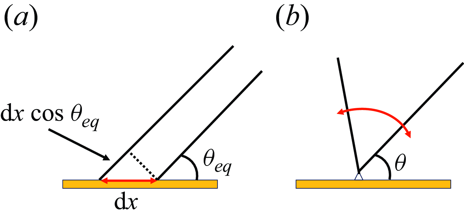

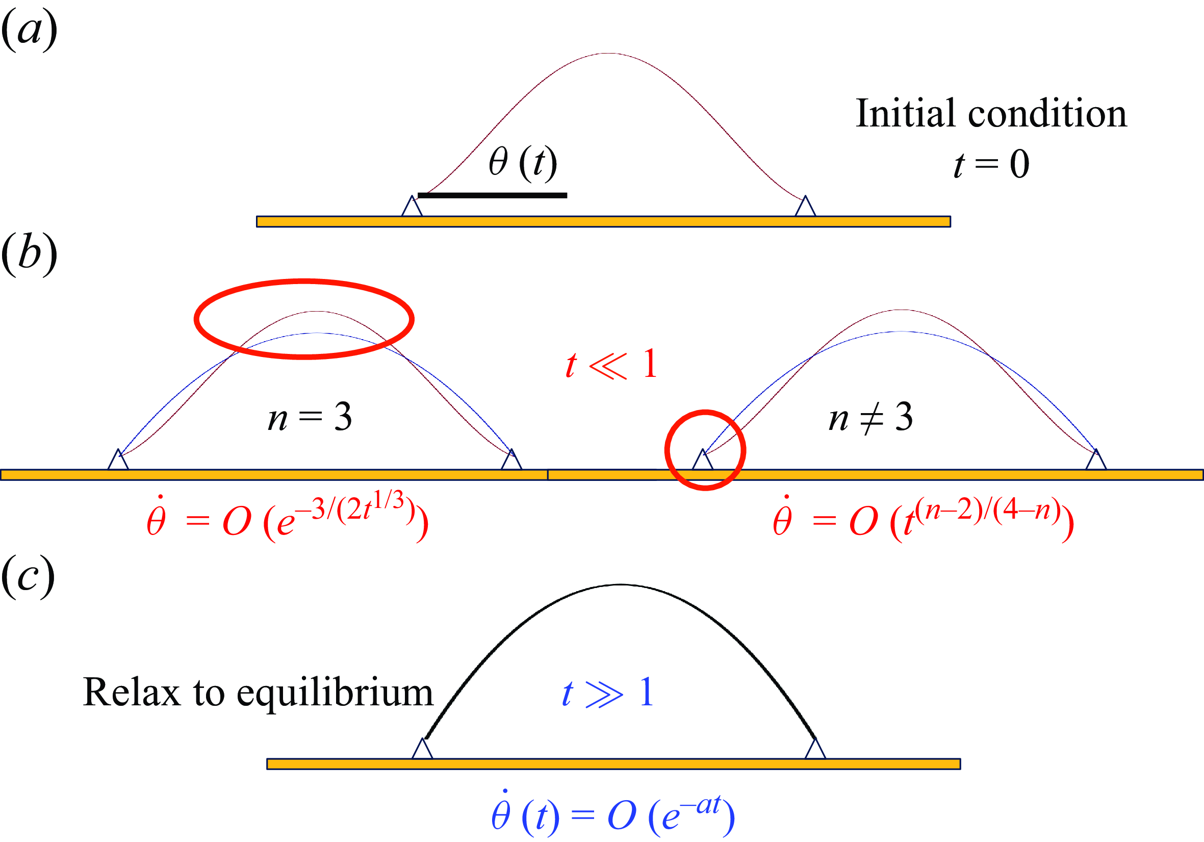


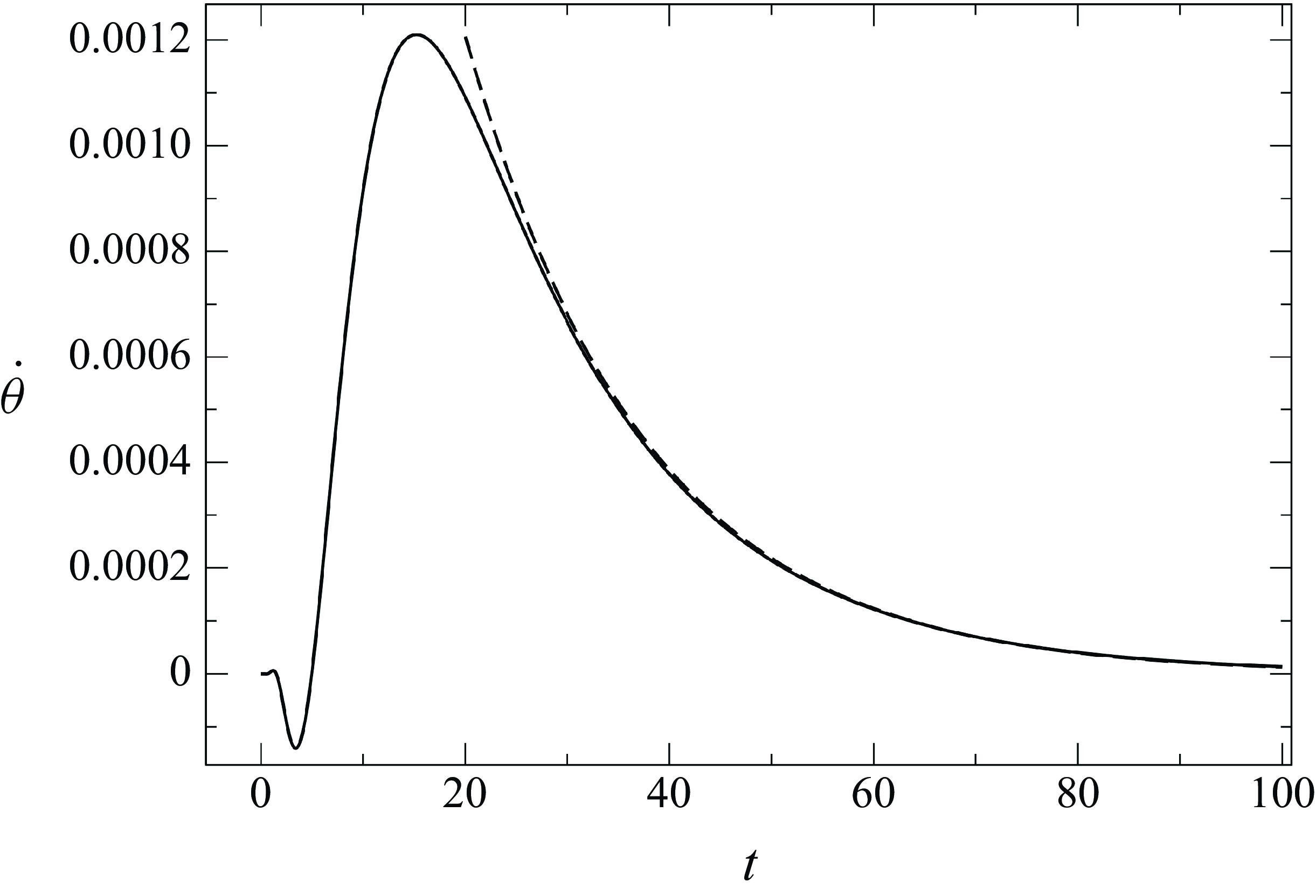


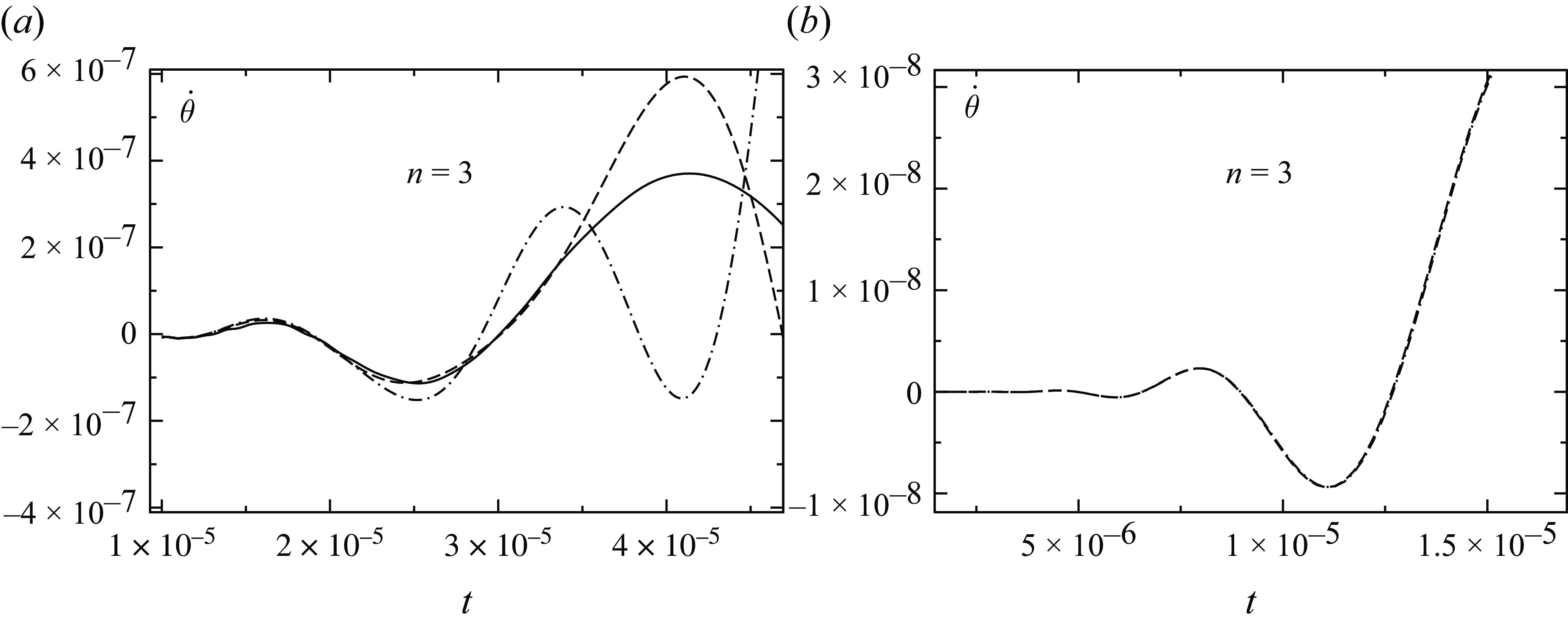


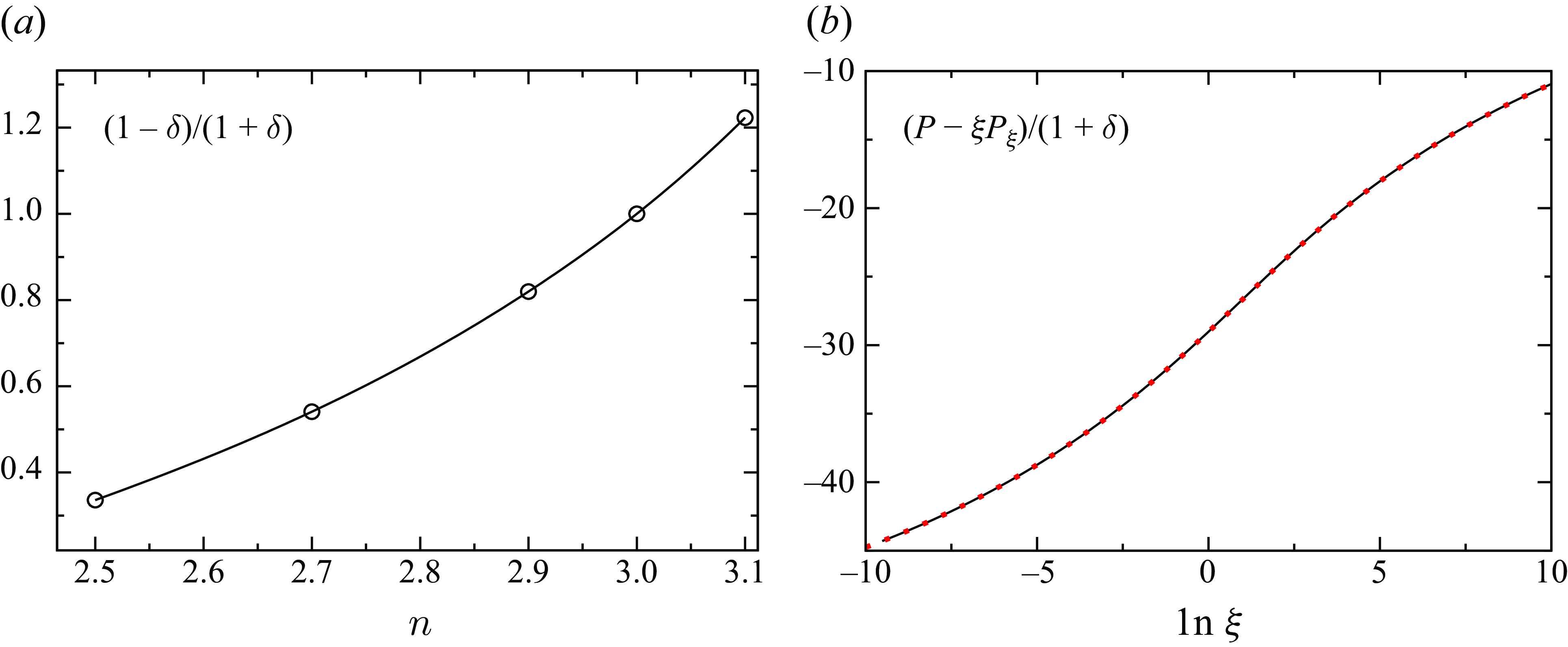


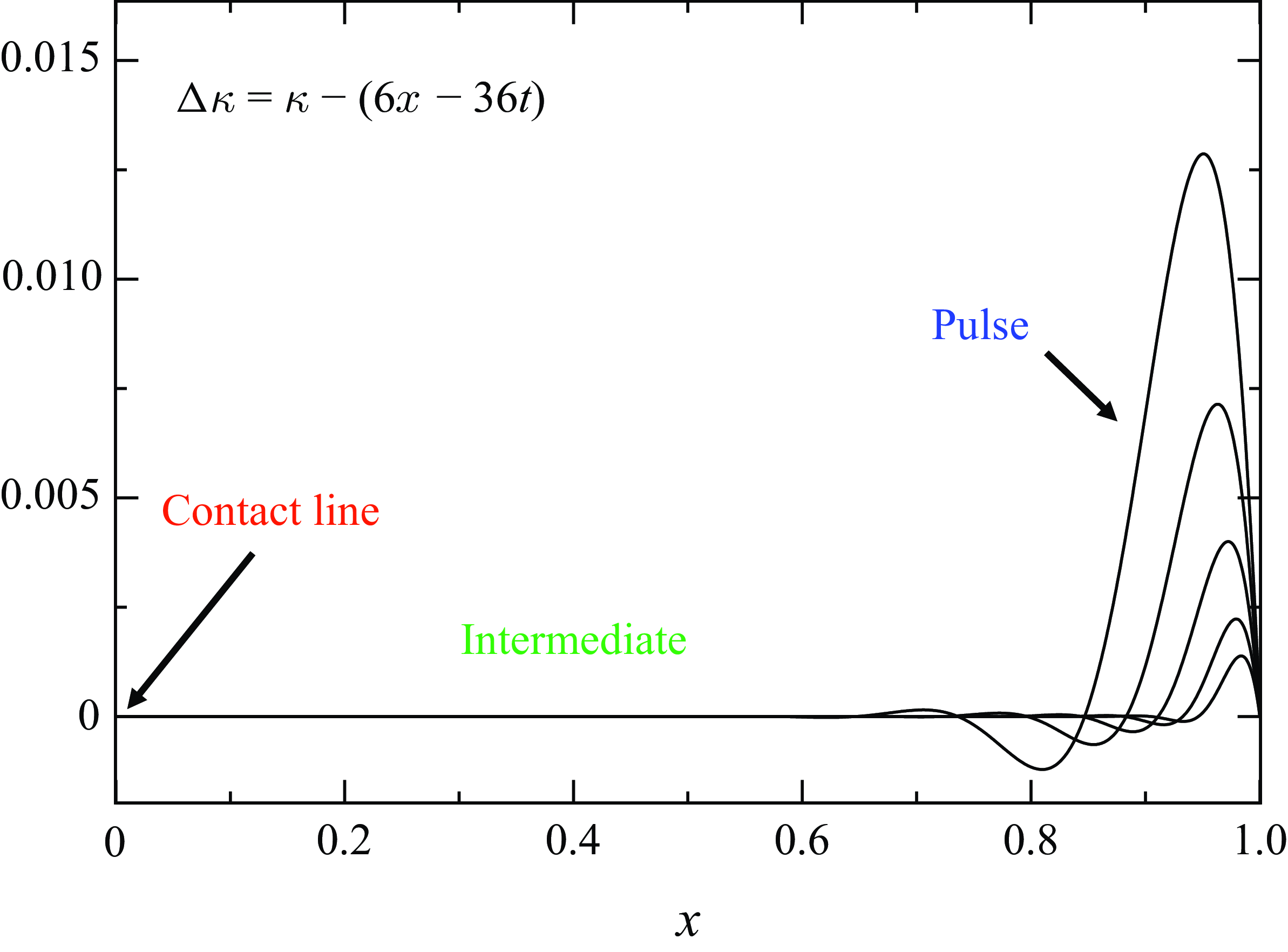


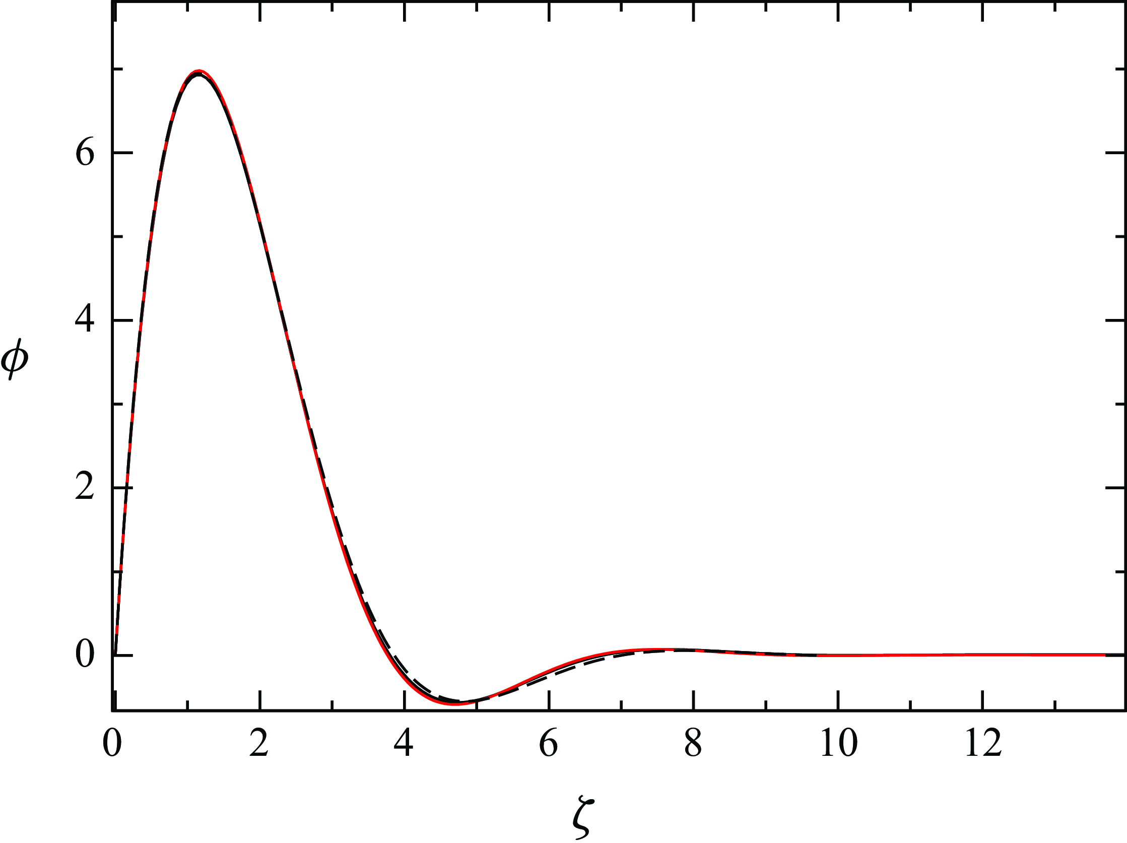


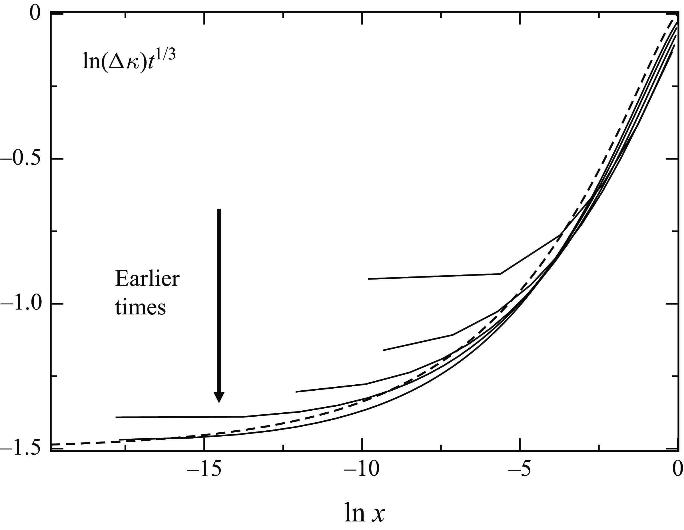


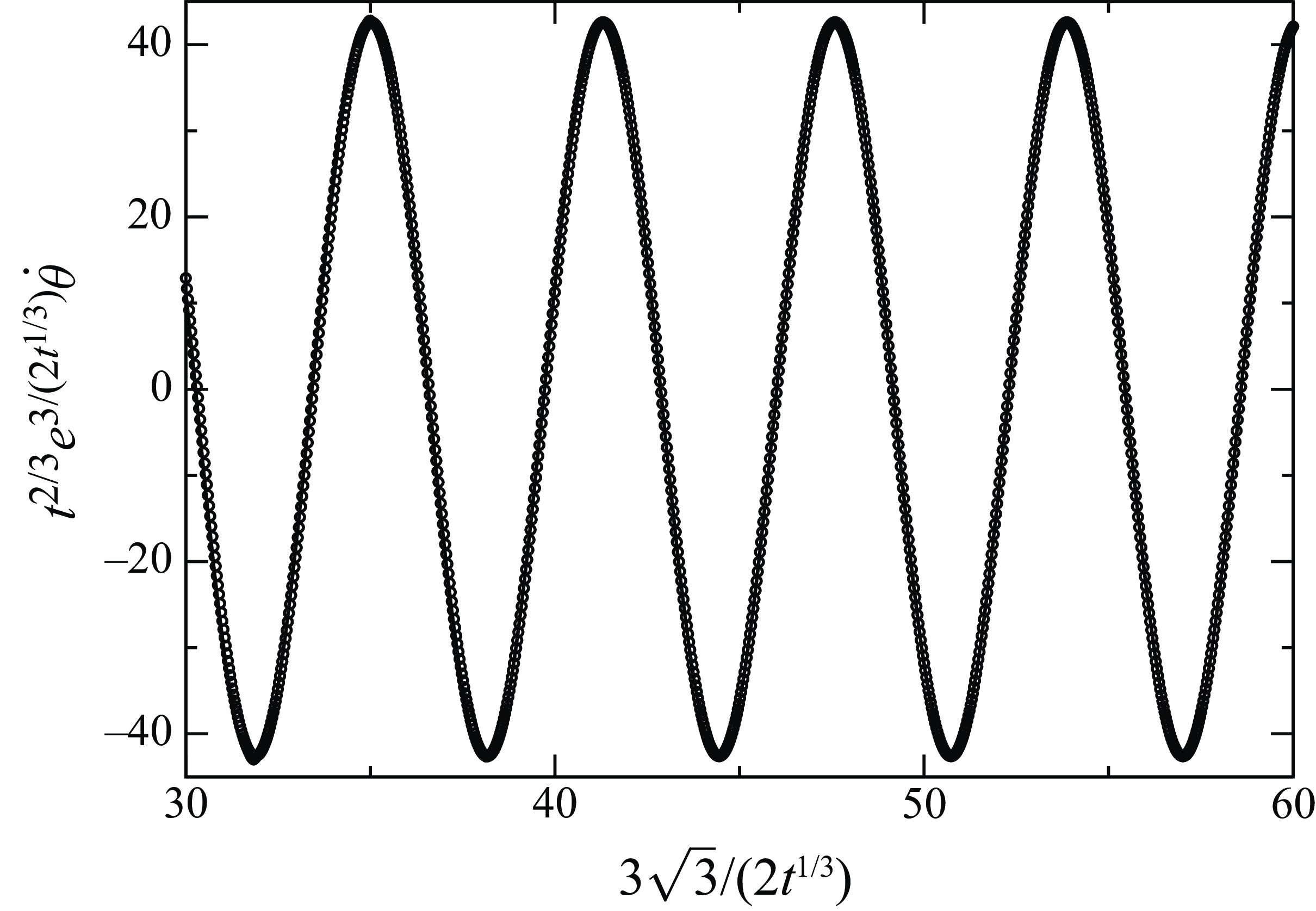


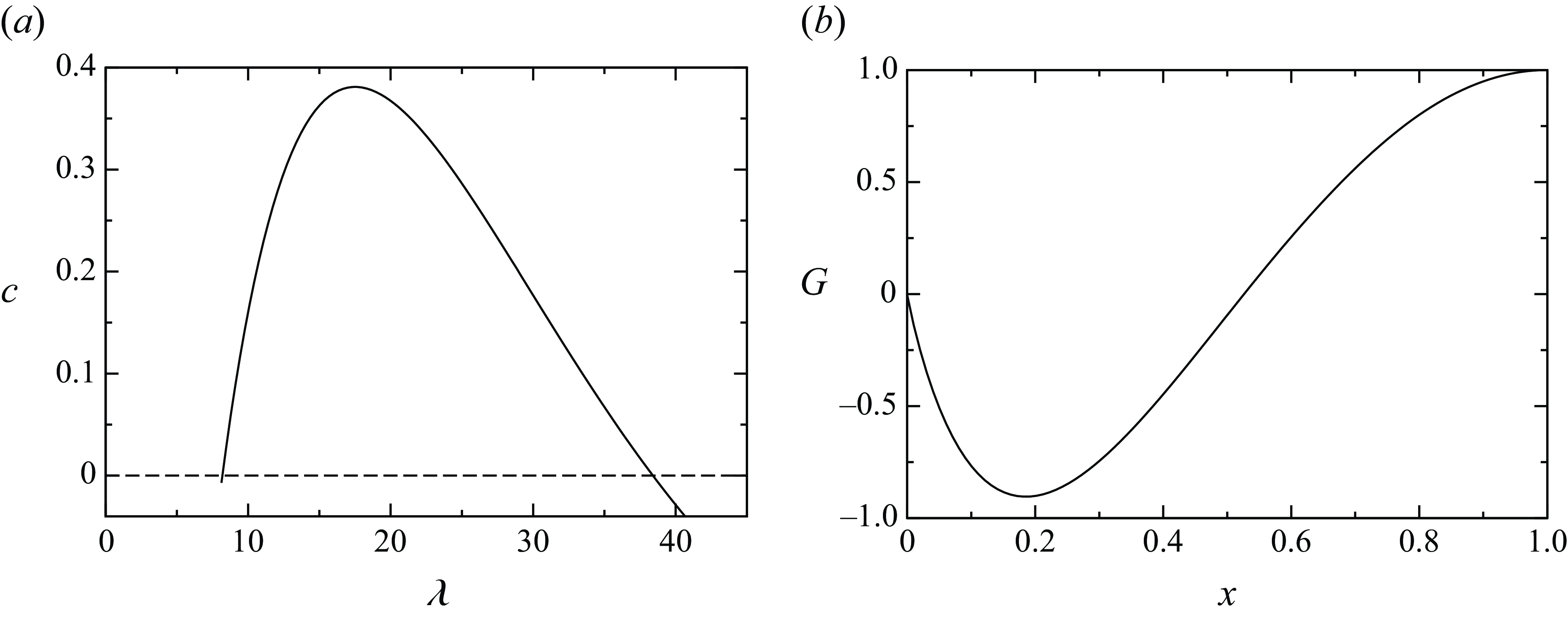


 Open access

