

1 Introduction
1.1 A new perspective on the development from -(e)th to -(e)s
This article aims to shed new light on the development of the third-person singular present tense suffix from an interdental fricative, as in giveth, to an alveolar fricative, as in gives. This morphophonemic sound change is not paralleled in lexical items; the fricatives in forms such as breath or youth obviously did not change. The development took place during the transition from Late Middle English to Early Modern English; the period focused on in this article is the time between 1417 and 1681, after which the alveolar suffix had largely ousted its former competitor.
A number of previous studies have addressed this topic (Holmqvist Reference Holmqvist1922; Stein Reference Stein1987; Lutz Reference Lutz1991; Kytö Reference Kytö1993; Ogura & Wang Reference Ogura, Wang and Britton1996; Nevalainen & Raumolin-Brunberg Reference Nevalainen, Raumolin-Brunberg, Dalton-Puffer and Ritt2000a, Reference Nevalainen and Raumolin-Brunberg2003) and identified several explanatory variables that are argued to correlate with the gradual replacement of -(e)th by -(e)s. These represent language-internal as well as language-external variables, including phonological factors, regional and social factors, variables of text type, as well as frequency.
A central phonological factor concerns verbs with stem-final sibilants such as kiss, judge or arch, which did not undergo the change as readily as other verbs (Kytö Reference Kytö1993: 130). Presumably, this can be interpreted as the result of speakers trying to avoid a close sequence of auditorily similar sounds (cf. the horror aequi principle, Rohdenburg Reference Rohdenburg, Rohdenburg and Mondorf2003). Stem-final alveolar stops are sometimes discussed as having a similar effect, but there is no clear consensus whether this effect actually obtains (cf. Kytö Reference Kytö1993: 130; Ogura & Wang Reference Ogura, Wang and Britton1996: 124).
Geographically, the development spread from Northumbria throughout the rest of England, affecting London towards the end of the fifteenth century and East Anglia in the early seventeenth century (Holmqvist Reference Holmqvist1922; Nevalainen & Raumolin-Brunberg Reference Nevalainen, Raumolin-Brunberg, Dalton-Puffer and Ritt2000a).
The factor of gender is of importance as well. Kytö (Reference Kytö1993: 129) presents evidence to suggest that the transition from -(e)th to -(e)s conforms to the pervasive tendency of women typically being at the forefront of linguistic change. During the sixteenth and early seventeenth century, women show a higher rate of the alveolar suffix. Nevalainen & Raumolin-Brunberg (Reference Nevalainen and Raumolin-Brunberg2003: 195) offer converging evidence, further showing that the gender difference neutralizes in the mid seventeenth century.
The social stratification of the development is also taken up by Nevalainen & Raumolin-Brunberg (Reference Nevalainen and Raumolin-Brunberg2003: 144), who distinguish between four classes: upper, social aspirers, middle and lower. Whereas middle-class writers show the highest ratio of alveolar suffix usage during the fifteenth and early sixteenth century, they are superseded by the lower ranks in the later sixteenth century. After 1620, social differences are no longer recognizable. The new alveolar variant thus entered the grammar of English as ‘a common suffix among the lower orders’ (Reference Nevalainen and Raumolin-Brunberg2003: 145).
Text type is discussed as a predictor variable by Kytö (Reference Kytö1993: 132). Early usages of the alveolar variant are found at a relatively higher rate in informal genres, such as private letters. However, Kytö points out that formality is no longer an important factor after 1640, and it never figures in her data of American English. Nevalainen & Raumolin-Brunberg confirm the secondary status of text type as a factor involved in the change from -(e)th to -(e)s in British English (Reference Nevalainen and Raumolin-Brunberg2003: 195).
The variable of register is studied by Nevalainen & Raumolin-Brunberg (Reference Nevalainen and Raumolin-Brunberg2003: 195), who operationalize it by comparing letters written to family and friends against letters written to recipients outside the family. While one might hypothesize that the progressive variant occurs more often in relatively intimate, informal contexts, Nevalainen & Raumolin-Brunberg report that the effect of register is minor and that it even shifts its direction over time.
Finally, the verbs do, have and say lag behind other verbs in their occurrence with the new alveolar suffix. Since it is well known that highly frequent items tend to be conservative (Bybee Reference Bybee2002, Reference Bybee2006), the role of frequency in the development from -(e)th to -(e)s needs to be taken into account. In fact, Ogura & Wang (Reference Ogura, Wang and Britton1996: 121) consider frequency to be the most important factor in the development, which they see as an instance of lexical diffusion.
Given that the development from -(e)th to -(e)s has attracted a good deal of attention, why is there a need for yet another study? In our view, several methodological reasons call for a new perspective on the phenomenon in question. First, most studies mentioned above limit themselves to essentially monofactorial designs, analyzing one variable at a time. It is, however, essential to control simultaneously for the effects of all relevant variables if one wants to be certain that a given variable has a genuine effect that is not the by-product of other variables.
One of the references cited above, Nevalainen & Raumolin-Brunberg (Reference Nevalainen and Raumolin-Brunberg2003), does address this challenge and presents a multivariate analysis. Using Varbrul (cf. Paolillo Reference Paolillo2002), they contrast three forty-year periods with regard to three language-external factors: region, gender and register. The analysis establishes that of these three factors, region has the strongest predictive power throughout, which reflects the regional spread of the alveolar suffix from the North to London and the rest of England. Gender differences are important during the first two periods, with women writers leading the change, but as mentioned above, these differences disappear in the mid seventeenth century. Across the three time periods, the factor of register has only minor predictive power.
The approach presented in this article shares substantial common ground with the study by Nevalainen & Raumolin-Brunberg (Reference Nevalainen and Raumolin-Brunberg2003), but departs from it in several crucial ways. First, it stands to reason that a simultaneous analysis of language-internal and language-external factors would greatly enhance our understanding of the historical process.
Second, instead of conducting separate analyses for sequential time periods, which are then inspected for comparison, we would like to conduct an analysis in which the passage of time is but one explanatory variable among others. In a case like the one at hand, the analysis would detect a trivial main effect of time – as time progresses, the rate of the alveolar suffix increases. Importantly and non-trivially, however, the inclusion of time as an explanatory variable allows us to study how the remaining variables interact with it. As suggested in the analyses by Kytö (Reference Kytö1993) and Nevalainen & Raumolin-Brunberg (Reference Nevalainen and Raumolin-Brunberg2003), some factors are in effect only at certain times. We would like to find out when exactly the gender difference ceased to be important or when verbs with stem-final sibilants finally adopted the alveolar suffix to the full extent. Previous studies have assessed these developments qualitatively, but again it stands to reason that the ability to determine significance values for interactions of the type described above would be useful.
Third, all studies mentioned above group their diachronic data into pre-defined historical stages. Kytö (Reference Kytö1993) and Ogura & Wang (Reference Ogura, Wang and Britton1996) use the established seventy-year time periods of the Helsinki corpus (see Kytö Reference Kytö1996); Nevalainen & Raumolin-Brunberg (Reference Nevalainen and Raumolin-Brunberg2003) partition their data into forty-year and twenty-year time slices for different analytical purposes. While this is a standard practice in the field that is rarely reflected upon, it is problematic: given the heterogeneous nature of diachronic corpus data, partitioning data into periods of twenty, forty or seventy years may lead to different interpretations of the data regarding the presence or absence of trends, the slope of trends and the position of turning points. Since the time periods of corpora such as the Helsinki corpus have been chosen on the basis of solid insights about the history of English at large, they constitute average reference points, but they cannot by design provide the optimal temporal classification for each of the many thousand linguistic phenomena one may want to study. To alleviate this problem, Gries & Hilpert (Reference Gries and Hilpert2008) propose a bottom-up method for the identification of stages in diachronic corpus data. We adopt this method here, discussing it further in section 2, and we submit that the data-driven partitioning of diachronic data is a highly important preparatory step for any diachronic analysis of corpus data.
The fourth and final reason for our reconsideration of the change from -(e)th to -(e)s is the fact that some potentially relevant factors have been disregarded in previous accounts. For instance, a phonological horror aequi effect similar to the one mentioned above concerns the onset of the word that follows the verb form. If the word to the immediate right of the verb form begins with an alveolar fricative or an interdental fricative, speakers might be biased towards choosing the variant that will avoid a repetition of identical sounds. To illustrate, he gives thanks should be preferred over he giveth thanks. Our analysis thus registers whether the first right collocate begins with an interdental or alveolar fricative, or with some other phoneme.
A second factor concerns gender. In a study of dramatic dialogue, Biber & Burges (Reference Biber and Burges2000) find an interaction effect between speaker gender and recipient gender. Differences between cross-gender talk and same-gender talk may well have been a factor in the change from -(e)th to -(e)s as well. Since our corpus consists of letters for which the gender of both sender and addressee is known, we include both as variables in our analysis.
Another factor that has not been considered is morphosyntactic priming. Much evidence suggests that hearing or producing a linguistic form once biases speakers towards producing that form again (Pickering & Branigan Reference Pickering and Branigan1998; Gries Reference Gries2005; Szmrecsanyi Reference Szmrecsanyi2006). In concrete terms, if a writer uses the interdental suffix early on in a sentence, the following third-person singular forms have an increased likelihood of being formed with that variant as well. Our analysis thus registers the presence of potential primes.
Lastly, virtually all accounts affirm the existence of speaker idiosyncrasies. Variation is observed across different speakers as well as within speakers. Some contemporary writers show markedly different patterns, some writers change over time, some largely retain the conservative interdental variant throughout their lives. These sources of variation do, however, remain unaccounted for in the studies that we have surveyed. In our view, currently the best way to address this issue is to use generalized linear mixed-effects modeling (Bates & Maechler Reference Bates and Maechler2009), which allows a treatment of speaker idiosyncrasies as so-called random factors. We discuss this further in section 3.
In summary then, the present article has two main goals. First, we want to stress the importance of partitioning diachronic corpus data in a bottom-up, data-driven way, and we are exemplifying the use of a tool for this purpose. Given that many resources of this kind are currently being made available (see Beal et al. Reference Beal, Corrigan and Moisl2007), and more analytical methods for historical developments are being developed (Hinneburg et al. Reference Hinneburg, Mannila, Kaislaniemi, Nevalainen and Raumolin-Brunberg2007; Hilpert & Gries Reference Hilpert and Gries2009b), the need for sensitivity towards this issue appears evident. Second, we present an analysis of a morphophonemic change that draws on prior insights, but adds factors that were previously not accounted for, applying a statistical methodology that is in several ways more sensitive and reliable than what has been available to earlier studies.
1.2 Methodological preliminaries
While diachronic corpus data are a valuable resource for investigating linguistic variation over time, there are quite a few challenges that arise from the phenomena as well as the data involved.
One such challenge is that, while trends and developments are most easily discovered and quantitatively describable when they are long-lasting as well as monotonous/linear, the reality is that such ‘convenient’ trends are the rare exception rather than the rule. Rather, diachronic developments often occur in interrupted spurts over short time spans and involve complex nonlinear relationships between variables.
Another, maybe even more fundamental, challenge is more directly concerned with the data itself. Corpora are always incomplete models of some linguistic reality, but they are of course particularly imperfect when it comes to diachronic data. That is to say, they are spotty in the sense of covering only particular genres, particular kinds of authors, particular kinds of dialects, and while diachronic corpus compilers have undertaken huge efforts, the very fact that we are dealing with an ultimately finite sample of data from the past makes it impossible to even approach the sizes and degrees of representativity of data that synchronic studies of PDE can utilize. As a result, developments and trends are not only difficult to characterize for the reasons mentioned in the previous paragraph, they are also, by virtue of the data problems, less reliable given the inherent limitations of diachronic corpus compilation.
Both of these challenges come together in undesirable ways. For instance, many studies do not quite do justice to the complexity and multifactorial nature of the phenomena but rather adopt coarser, less objective and less revealing monofactorial methods (see our discussion in section 1.1). In addition, some studies do take a multifactorial approach, but then use tools that are not up-to-date and powerful enough anymore; as we will argue in more detail in section 3 below, the use of Varbrul is a case in point. Finally, many studies do not adopt techniques to come to grips with the huge variability of diachronic corpora, variability that arises both within one corpus and between corpora (such as when different corpora have to be combined to obtain data covering a larger time frame than a single corpus can provide).
In the present article, we attempt to address these issues. By way of a case study, we exemplify two newly developed methods, variability-based neighbor clustering (e.g. Gries & Hilpert Reference Gries and Hilpert2008) and generalized linear mixed-effects modeling (e.g. Baayen Reference Baayen2008: ch. 7), which can substantially increase adequacy and accuracy of the study of historical change in general, and of the change from -(e)th to -(e)s in particular. Using these methods we will identify temporal stages in which the change of the third-person singular form took place as well as the factors that are correlated with, and hence presumably drove, this change. Crucially, both methods are to a very large extent data-driven, replicable (i.e. they involve very little debatable intuition on the part of an analyst), and comparable to quantitative methods that have proven their worth in other fields.
1.3 The data
In order to study the shift from -(e)th to -(e)s over time, we used data from the Parsed Corpus of Early English Correspondence (PCEEC; see PCEEC 2006, Nevalainen & Raumolin-Brunberg Reference Nevalainen, Raumolin-Brunberg, Nevalainen and Raumolin-Brunberg1996). More specifically, we retrieved 13,007 cases of -(e)th and 7,437 cases of -(e)s, including spelling variants; the data come from 233 different years between 1417 and 1681. While the choice of this corpus restricts us to a single text type, its annotation gives us access to the precise year in which each example was produced. Also, we learn about the gender of both writer and addressee, as well as their mutual relation.Footnote 2 Given that previous studies view text type as a minor determinant of the alternation, the PCEEC was our best option for the task at hand.
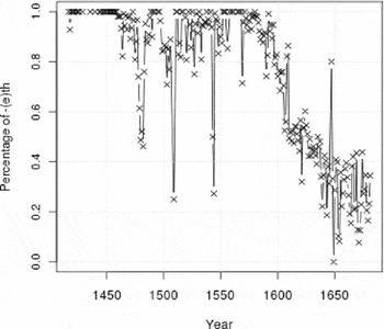
When the proportions of -(e)th are plotted against time, there is a clear overall decreasing trend, as is shown in figure 1. However, it is also clear that the trend is characterized by several marked outliers. While these outliers do not undermine the general decreasing trend of -(e)th, they make a further quantitative analysis of the data much more problematic. If one applied regression methods in general, but especially linear regressions, to such data, the computations of coefficients, effect sizes, and p-values would suffer a great deal from the regression's attempt to determine coefficients that take outliers into consideration, so the outliers will introduce considerable bias into the statistical analysis. While it would be desirable to be able to omit some obvious outliers from the analysis, the desire for cleaner data is counterbalanced by a need to be true to the data and not just delete whatever data points do not fit a trend derived from eyeballing a plot of relative frequencies. What is needed is a principled method that conservatively identifies data points as outliers and at the same time identifies coherent temporal stages in the data in an objective and replicable way. The next section outlines such a method and its application to the data.
Proportions of -(e)th against time in the PCEEC

2 Identifying stages of temporal development
Given the huge variability of the 233 different recordings, we decided to group these recordings into temporal groups that are characterized by a high degree of within-group similarity and a low degree of between-group similarity. On the one hand, this allowed us to reduce the number of values/levels we need to distinguish in our analysis (from 233 to a much smaller number); on the other hand, this also allowed us to identify and discard outlier values which would otherwise have rendered the identification and interpretation of any diachronic trends very difficult.
These requirements and goals already strongly suggest a bottom-up/data-driven hierarchical agglomerative clustering approach, but it is necessary to point out that the regular kinds of such clustering approaches are not applicable here. The main reason for this is that regular clustering approaches are blind to the temporal order of elements. As Gries & Hilpert (Reference Gries and Hilpert2008) and Gries & Stoll (Reference Gries and Stoll2009) argue and exemplify, if the common kind of clustering algorithm is applied to temporally ordered data (such as historical or language acquisition data), then the algorithm may group data from very different time periods together, which may result in the algorithm creating clusters that
– contain writing whose date of creation may differ by 500 years, which does not make sense given the huge linguistic changes that will have taken place during this time;
– contain recorded speech whose dates of recording may differ by 3.5 years, which does not make sense given the immense cognitive and linguistic development that children exhibit during such time.
The above-mentioned publications present a new clustering algorithm called VNC (for variability-based neighbor clustering) that is conceptually similar to existing hierarchical agglomerative approaches, but operates under the restriction that only temporally adjacent files/recordings can be merged, which prohibits the kind of nonsensical clusters that group together similar data points from non-adjacent time periods.Footnote 3 We do not discuss the general specifics of the VNC algorithm here in much detail, referring the reader to the above publications, but the following two sections discuss how the VNC algorithm was applied to our data and what temporal stages we arrived at.
2.1 Methods
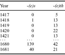
The VNC approach involves an iterative algorithm that amalgamates the 233 temporally disparate recordings into successively larger groups/clusters.Footnote 4 The input to the VNC algorithm is a table of the kind exemplified in table 1.
Input data to the VNC algorithm
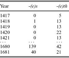
The VNC algorithm then proceeds as follows. First, the algorithm computes the percentage of -(e)s out of all -(e)s and -(e)th in the temporally earliest file, the percentage of -(e)s out of all -(e)s and -(e)th in the temporally next file, and, crucially, the standard deviation of the two percentages (as a measure of their similarity). For 1417, the proportion of -(e)th is 0 percent, for 1418, the proportion of -(e)s is 92.86 percent, etc. This procedure is repeated for all temporally adjacent pairs of files; i.e. for all 232 adjacency pairs of 233 files.
Second, the algorithm determines which of all the computed standard deviations is the smallest, indicating the two most similar files, in this case 1419 and 1420, which both exhibit a proportion of -(e)th of 100 percent.
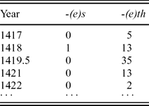
Third, the algorithm amalgamates the two most similar files by summing the frequencies observed in the original two files, replaces the years of creation of the original two files by their mean, yielding table 2, and memorizes the standard deviation of the two merged files (0, in this case) as a measure of their difference.
First amalgamation of the VNC algorithm
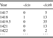
The algorithm then iterates, i.e. repeats the above three steps another 231 times (i.e. 232 times altogether) until all 233 files have been merged into a single cluster and all 232 standard deviations of amalgamated clusters have been recorded.
2.2 Results
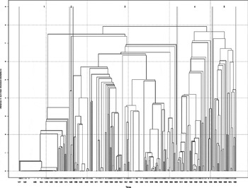
This process yields two kinds of plottable results. On the one hand, one can plot the standard deviations arising during the amalgamations in reverse order to obtain what in the context of principal components analysis is known as a scree plot and which facilitates the identification of how many clusters to assume. On the other hand, one can generate the familiar kind of dendrogram that reflects how similar (clusters of) recordings are to each other.
Our first step was to use this approach to identify outliers in the data, following the discussion in Gries & Hilpert (Reference Hilpert2008: 77). On the basis of the first dendrogram, the files for 1509 and 1544 were omitted because these two files instantiated the only clusters that consisted of only one individual file respectively, and their -(e)s percentages were vastly exceeding those of the files around them; they could thus safely be regarded as outliers.
In much the same way that model selection processes in the domain of general(ized) linear modeling are performed, we then performed a second VNC analysis to see to what degree the first deletion of outliers improved the homogeneity of the data. This second VNC dendrogram led to the deletion of another outlier file for the year 1649, which again instantiated a single-file cluster with a very atypical -(e)s percentage.
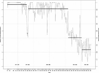
A third VNC dendrogram then yielded a structure that was fairly regular and homogeneous, but at the same time left us with a difficult choice: out of a total of five clusters, the second one covered only a very short time span (four years) and showed a surprisingly high rate of -(e)s that exceeded the rate of the third cluster. On the one hand, we could have eliminated this cluster because (i) it is the only obstacle to an otherwise perfectly monotonous increase in the proportion of of -(e)s over time, (ii) it is a small cluster of only four years, and (iii) one-third of the data in that cluster are from a writer behaving rather atypically when compared to the rest of the writers (Richard Cely Jr). On the other hand, we felt obliged to leave this cluster in because, unlike the other eliminated outliers, this cluster does cover more than just a single year. While the first option appeared tempting, we opted for the second one, because while VNC-like approaches have been applied in several case studies now – Gries & Hilpert (Reference Gries and Hilpert2008), Gries & Stoll (Reference Gries and Stoll2009), Hilpert & Gries (Reference Hilpert and Gries2009a) and Baker (to appear) – it is still a relatively recent method. We therefore chose to err on the conservative side, conservative in the sense of not imposing structure on the data ourselves and avoiding the accusation of using outlier deletion to make our data exhibit a nice monotonous trend. Once VNC is more established, we and other researchers will feel more self-confident to use prior knowledge and expertise together with the data-driven results to determine the best possible course of analysis.
The 233−3 = 230 time periods that survived the outlier deletion (i.e. still 98+ percent of the original data) were grouped into clusters as indicated in table 3; see appendix A for graphs summarizing the results of the VNC. The data on the change from -(e)th to -(e)s were then recoded such that instead of the years of the individual files, we used the five VNC periods.
Time periods identified by the VNC algorithm

At this point, it may prove useful to connect back to a point made in the introduction and to discuss briefly what we see as the advantages of relying on VNC-generated time periods rather than taking the pre-defined historical periods of diachronic corpora.
A first advantage is that the VNC periods are derived directly from the phenomenon under investigation. If we study a certain grammatical form, it is clear that the development of this form need not coincide with general periods of the English language at large. This holds true especially for developments such as the change from -(e)th to -(e)s, which takes place at the transition from Middle English to Early Modern English. In other words, VNC can provide temporal stages that are more fine-tuned to a specific phenomenon at hand.
Also, grammatical changes need not conform to time periods of even lengths. There may be extended periods of stasis followed by short spurts, and these divergent developments will be more fruitfully analyzed as separate periods, even if they fall within the same seventy-year span. Reliance on pre-defined corpus periods may thus obscure or distort trends that are present in the data. Naturally, these issues will become apparent to researchers who group their diachronic data into time slices of different lengths and conduct multiple analyses, but instead of such a manual trial-and-error process, VNC offers an alternative by determining periods that ‘make sense’ in a bottom-up, data-driven way. Hence, VNC can make an otherwise labor-intensive and inherently subjective decision process more transparent.
A third advantage is of course that VNC enables the analyst to identify and discard outliers in an objective fashion, as illustrated above. To our knowledge, there are no established procedures that would handle this problem, despite the fact that it is ubiquitous in diachronic corpus research.
A fourth clarificational comment has been prompted by an anonymous reviewer who suggested that it would ‘be interesting to test whether the results stay the same if the granularity of timing the data is changed from 1 year to 5 or 10 years’. We agree that that would indeed be interesting, but submit that it would go beyond our aims for the present study. If we wanted to rerun the analysis, we would have to decide on a particular level of granularity, as when the reviewer suggests using five or ten years. These two suggestions are obviously motivated more by the fact that we use a decimal system rather than by any linguistic or theoretical consideration, which is why these suggestions embody exactly the kind of a priori convenience classification that we argue against here. There are two ways to handle this which do not suffer from this arbitrariness problem and follow the reviewer's suggestion, but they both run counter to the data-driven approach that is adopted here:
– one way to implement the reviewer's suggestion involves grouping the data before the application of VNC: we could systematically vary the level of granularity from, say, one year (the present approach) to twenty years, run VNC on each of these solutions, decide on a number of clusters, and then rerun the GLMEM modeling and see how the results change. However, this would turn the article into a purely quantitative Monte Carlo simulation type of experimental study for a very different audience;
– the other way involves grouping the data after and on the basis of VNC: we could inspect the current cluster solution, where we decided on five clusters and identify a number of clusters that contain the numbers of years that come close to the reviewer's suggestion. However, this raises two problems. First, there are very many different clusterings that will come close to the reviewer's proposed level of granularity and there's no way to know which one gives the results best suited for the comparison intended by the reviewer. Second, this approach would very much undermine the bottom-power of VNC: we decided in favor of five clusters on the basis of an analogon to the scree plot used in principal component/factor analyses, i.e. we chose a number of clusters that result in the best local discriminatory power. If one did not do that and chose, say, fifty clusters instead, the results would of course be different, but any discrepancy between the present findings and the hypothetical fifty clusters could not be interpreted as supporting or undermining VNC because the decision on the number of clusters was not made in accordance with the VNC approach.
For these reasons, we only pursue the present approach and leave the systematic exploratory study of VNC's properties for future research.
To sum up, while pre-defined corpus periods will not necessarily yield a false or distorted view of grammatical developments, they are by definition likely to distort, or gloss over, developments. By contrast VNC can warrant a level of empirical adequacy that makes it a desirable choice. A sceptic might of course argue that the finest possible granularity will always be the most informative. Why do we not simply keep the year-based distinction of 233 time periods? While our (verb-form-based) classification of the corpus into temporal stages makes the data more manageable than the original (year-based) classification, we still lose some, and maybe too much, information because our creation of stages turns an interval-scaled variable (year) into an ordinal or, as we used it, categorical variable VNCPeriod.Footnote 5 To address this issue, we ran one logistic regression trying to predict the verb form based on our five VNC-based stages (as a categorical factor) and one logistic regression trying to predict the verb form on the basis of the year in which the letter was written. It turns out that the regression based on the VNC stages is more successful (Gamma = 0.811, Nagelkerke's R 2 = 0.46) than the regression based on the year (Gamma = 0.675, Nagelkerke's R 2 = 0.37) even if the three outlier years, which would have made the regression even worse, have already been removed. We therefore submit that the results of our clustering approach are in fact a suitable approach to including temporal information into the regression models to be discussed below.
3 Exploring the shift from /θ/interdental to /s/alveolar
After the temporally ordered data were cleaned from a few outliers and grouped into internally coherent temporal stages in a data-driven way, we set out to investigate the way in which the change from -(e)th to -(e)s took place over time and which variables determined the developments most strongly and significantly.
A frequently used tool in variationist studies of both historical change and (second) language acquisition is Varbrul (Berdan Reference Berdan, Bayley and Preston1996; Nevalainen Reference Nevalainen2000; Nevalainen & Raumolin-Brunberg Reference Nevalainen and Raumolin-Brunberg2003, inter alia). However, while Varbrul has been applied in this area of study, a standard textbook on Varbrul actually discourages uses of this type for the simple reason that continuous independent variables cannot be handled adequately (Paolillo Reference Paolillo2002: 15–16). For our analysis, we decided to use a method that is based on binary logistic regression but goes beyond it in several respects: generalized linear mixed-effects modeling, GLMEM, for which we used the the lme4 package in R (see Bates & Maechler Reference Bates and Maechler2009 and R Development Core Team 2009 respectively).
Similar to Varbrul, both binary logistic regression and our GLMEM are used to predict the outcome of a binary dependent variable on the basis of several predictors. However, both these methods are superior to Varbrul in the following ways: binary logistic regression and GLMEM
– can easily handle categorical and continuous predictor variables (without factorization);
– can easily handle interactions of different kinds of predictors;
– are part of comprehensive theoretical statistical models (generalized linear models and mixed-effects/multilevel models) that are based on widely used statistical algorithms and, therefore, produce output that can be straightforwardly compared with other approaches.
GLMEM in particular has even more to offer, however. Its predictive power is usually much higher than that of Varbrul or binary logistic regression because what remains residual variation in those two techniques is used to improve the estimates of the regression coefficients. Unlike both Varbrul and binary logistic regression, GLMEM can
– identify patterns in the residual variation that can be attributed to characteristics of the studied elements on different levels of granularity. For example, GLMEM can include what in psycholinguistic studies has been referred to as by-subject/speaker or by-item variation (see Clark Reference Clark1973) or other kinds of variability or interrelations in the data that would otherwise just constitute residual deviance or violate the independence-of-data- points assumption of regressions;
– fine-tune its computation of regression coefficients by taking into consideration the amounts of data points contributed by different authors or involving different verbs (see Gelman & Hill Reference Gelman and Hill2006: 246, 254).Footnote 6
The following sections discuss how our verb forms and their contexts were annotated and analyzed statistically as well as the results of the statistical modeling process.
3.1 Methods
All the verb forms in our data were annotated with regard to a variety of variables. First and trivially, each verb form was annotated with regard to the variable Variant, which indicated which third-person singular form was used: -(e)s vs -(e)th.
Second, each verb form was annotated with regard to the following independent variables:
– VNCPeriod: the VNC periods obtained in section 2 for when the verb form was produced: 1 vs 2 vs 3 vs 4 vs 5;
– AuthGend: the gender of the author: male vs female;
– RecSameGender: is the recipient of the letter of the same gender as the writer: yes vs no;
– Priming: which suffix was used in the last verb form: -(e)s vs -(e)th vs other, to determine whether priming effects of the kind well documented for syntactic priming affect the choice of form;Footnote 7
– CloseFam: is the sender a close relative of the receiver: yes vs no;
– FinSib: does the verb stem end in a sibilant: yes vs no, to include a possible horror aequi effect;
– FolFric: does the following word begin in a fricative and if so what: s vs th vs other, to include a second possible horror aequi effect;
– Gram: is the verb in question a grammatical verb (i.e. auxiliary do or have): yes vs no.
The Gram variable is our way of operationalizating the factor of verb frequency, which has been identified as important in earlier accounts. We chose a simple categorical variable in this case, because a continuous variable would have to take account of lemma frequencies for all 885 verbs in all five VNC-periods, in order to control for verb frequency changes. In the interest of keeping our efforts manageable, we settled for a simpler solution.
In addition to establishing whether the variables described above have an effect, we also wanted to determine whether and how the forces of these variables shift during the change from -(e)s vs -(e)th over time. Statistically speaking, if one variable significantly affects speakers’ choices in an early corpus period, but not in later periods, then this variable interacts with the variable Time, and to be able to study these kinds of effects, we included the interactions of the above independent variables with VNCPeriod.
Third, one particularly interesting characteristic of GLMEM is the above-mentioned possibility to include additional higher-level characteristics of the use of each verb form. We included the following two variables as such random effects:
– Author: the name of the author who produced the verb form to obtain author-specific adjustments to intercept(s) (not to slopes) because, e.g. on the whole, John Jones uses a very high proportion of -(e)th (50 percent) whereas Winefrid Thimelby does not (6 percent), and these author-specific trends can be included in the analysis (our data come from 626 authors);
– Verb: the verb whose verb form is analyzed to obtain verb-specific adjustments to intercept(s) (not to slopes) because, e.g., the verb make has a fairly low occurrence of -(e)th (30 percent) while the verb know is attested with -(e)th (62 percent) much more; again, these trends can be included in the modeling process (our data involve 884 verbs).
Our choice of these two random effects is paralleled by the above-mentioned common practice in psycholinguistics to carry out separate by-subjects and by-items analyses and also takes into consideration the fact that the individual data points are not independent of each other.Footnote 8
Consider the example sentence in (1) as an example for our coding:
(1) So prayeth he that → promiseth ← always to be at your ladiship's command.
The use of promiseth in this sentence has been annotated as indicated in (2).
(2)


Once all verb forms were annotated this way, we used a stepwise GLMEM selection process to weed out insignificant predictors of the suffix variant. That is, we first iteratively fit a GLMEM with the above variables and deleted the least significant interaction of fixed effects until all variables and interactions in the model were either significant themselves or participated in a significant interaction. Then, we tested whether the adjustments to the intercept(s) of the random effects could be deleted from the model or not. Upon identification of the final minimal adequate model, we assessed the goodness of the fit, computed measures of classification accuracy, and inspected the coefficients to determine the directions and strengths of the significant effects, which will be discussed in the following section.
3.2 Results
The model selection process resulted in the successive deletion of several non-significant predictors in the order listed below:
– VNCPeriod × Priming (minimal p ≈ 0.45);
– VNCPeriod × AuthGend (minimal p ≈ 0.43);
– VNCPeriod × CloseFam (minimal p ≈ 0.06);
– CloseFam (minimal p ≈ 0.17).
The first of these translates into the result that there is no interaction between the passage of time and priming. In other words, there is no priming effect in one corpus period, only to be absent or reversed in another one. The same holds for author gender and close familiarity between author and recipient. Lastly, close familiarity between author and recipient does not figure as a main effect in our analysis, either.
Once these predictors were removed and only predictors remained that were significant themselves or that participated in significant interactions, it turned out that the two random effects could not be deleted, since their attempted deletion significantly decreased the model's performance (both p < 0.0001). Our final minimal adequate model is characterized by the following summary statistics:
– Log-likelihood = −3968; deviance = 7937;
– classification accuracy of our GLMEM with the two random effects: 94.43 percent;
– classification accuracy of our binary logistic regression without the two random effects: 86.14 percent.
In other words, the classification accuracy of the model is nearly perfect, since almost 95 percent of all verb forms are classified correctly, a value that is not only significantly different from the baseline (63.62 percent), but also significantly different from the already good classification accuracy of a binary logistic regression without random effects (86.14 percent) and very rarely achievable in the behavioral sciences. In the following two sections, we investigate the coefficients of the regression in more detail.
3.2.1 Fixed effects and their interactions: coefficients and interpretation
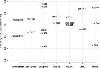
Since coefficients of generalized linear models are usually not exactly easy to understand, we summarize all effects graphically. Consider Figure 2 for all significant main effects. On the x-axis, we list all significant main effects, on the y-axis, we provide the probability of -(e)th (from 0 to 1), and in the main area we plot the variable levels of the significant main effects together with their averages of the predicted probabilities of -(e)th.
Average predicted probabilities of -(e)th for the levels of all significant main effects

That means, variable levels plotted above others are characteristic for -(e)th, whereas variable levels plotted in the lower half of the graph are characteristic for -(e)s. We thus see for instance that females show a greater tendency to use the alveolar suffix than men. Also recipient gender shows a main effect, as -(e)th is more likely to occur in same-gender writing. The data points above VNCPeriod illustrate the known effect of time – the interdental suffix occurs at a higher rate in earlier data. We observe horror aequi effects both with stem-final sibilants and following fricatives, and these effects are at very similar levels of magnitude. The grammatical verbs do and have expectedly occur more often with -(e)th than lexical verbs and finally, we see a strong priming effect in the expected direction.
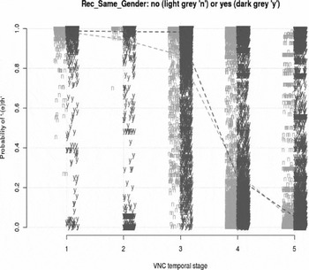
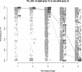
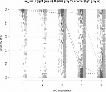
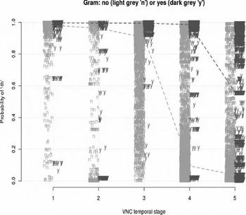
However, not all of these main effects can be taken at face value, given their significant interactions with the variable VNCPeriod, i.e. the dimension of time. For four independent variables, the model detected such interactions. These interactions – with RecSameGender, FinSib, FolFric and Gram – are represented in figures 3–6. For each panel, on the x-axis we represent the five VNC temporal stages (with time proceeding from left to right), and on each y-axis we represent the average predicted probability of -(e)th. For each figure, the levels of the variable whose interaction with VNCPeriod is represented are plotted with different letters and in different shading vertically (slightly jittered to the left and the right of an imaginary vertical line originating at the VNCPeriod number; given the massive overplotting of more than 20,000 data points, the points are also summarized by dashed non-parametric smoothers. For example, in figure 3 the levels of RecSameGender are no and yes, which are plotted for each of the five temporal stages with their (light grey and dark grey) initial letters n and y.
Average predicted probabilities of -(e)th for the interaction between VNCPeriod and RecSameGender

Average predicted probabilities of -(e)th for the interaction between VNCPeriod and FinSib

Average predicted probabilities of -(e)th for the interaction between VNCPeriod and FolFric

Average predicted probabilities of -(e)th for the interaction between VNCPeriod and Gram

Figure 3 shows that most of the time (in periods 1, 2, 4, and 5) it does not make a difference whether the sender writes to a recipient of the same gender or not. However, in period 3 (i.e. the sixteenth century), writers used -(e)s more often especially when writing to someone of the opposite sex. This is represented by a divergence of the two dashed lines – the lighter ‘cross-gender’ line slopes downwards whereas the ‘same-gender’ line stays horizontal. With this change in that period, the overall change is initiated, variation continues through period 4 and reaches completion for both kinds of recipients in period 5.
Figure 4 shows that the presence or absence of final sibilants in the verb in question did not play a role until period 4, i.e. the first half of the seventeenth century. In that period, the overall probability of -(e)th decreases considerably, but especially strongly for verbs that have no stem-final sibilant. That is, at this time, writers would already write, for instance, comes, but would continue to write forms such as causeth. In period 5, then, final sibilants again do not make a difference anymore; the change is largely completed at that time. The horror aequi effect of stem-final sibilants is thus operative only through a fairly short period of the change (~40 years), which is a surprising result that is in need of some explanation. We would suggest that a ‘soft’ constraint such as phonological horror aequi only becomes visible in the short temporal window when a new variant has become firmly established but has not yet ousted its predecessor. The fourth VNC period, in which -(e)th has a probability of occurrence that is near 0.5, represents that kind of temporal window.
In line with this reasoning, figure 5 indicates that the second horror aequi effect included in our analysis exhibits a fairly similar temporal profile. Again, the presence of a fricative at the beginning of the following word initially does not affect the choice of variant: -(e)th is preferred in general. In the first half of the seventeenth century (period 4), however, verb forms that are followed by words not beginning with an alveolar fricative exhibit a landslide tendency towards the newer variant, -(e)s, but it takes another fifty or so years (i.e. until period 5), until verb forms with a right collocate starting in /s/ catch up to exhibit the same strong preference for -(e)s. In other words, the alveolar suffix in a phrase such as Sam sings songs was avoided as long as possible.
Finally, figure 6 exhibits a similar time line of change. In periods 1, 2 and 3 both lexical and grammatical verbs strongly prefer -(e)th. However, even at these early times lexical verbs show a very slight tendency towards -(e)s while grammatical verbs (do, have) rather categorically stick to -(e)th. Again in period 4, then, lexical verbs make an extreme switch towards -(e)s, which continues (less strongly) throughout period 5. Grammatical verbs, however, continue to prefer -(e)th until the second half of the seventeenth century and begin to move towards -(e)s only then.
It emerges that the most dramatic changes arose during VNC periods 3 and 4, and these changes took place on several levels of linguistic analysis: sociolinguistically, writers began to adopt the newer form when writing to the opposite sex; phonologically, articulatory effects began to license the ascent of the new form; syntactically, (lower-frequency) lexical verbs began to give way to the new form. Again, it is worth pointing out that these kinds of effects and their confluence are not observable unless a multifactorial approach involving interactions with time is adopted.
3.2.2 Random effects: coefficients and comments
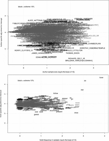
Let us finally also comment briefly on the random effects. We have already shown above that the random effects’ contributions to the final model are highly significant, but recall that those are not actually parameters of the regression model. Rather, they are ‘just’ author- and verb-specific adjustments to the intercepts of regression lines that are parameters within the model, i.e. the model's way of reducing variance otherwise unaccounted for. We will therefore not discuss the adjustments to the intercept, but only provide summary graphs that give a first indication of which authors and which verbs were in need of the largest adjustments.
In figure 7, we provide the author-specific and verb-specific adjustments in the upper and lower panel respectively. On the x-axis, we represent the frequency of data points from particular writers or with particular verbs; on the y-axis, we represent the size of the adjustment; the names of writers and the verbs are then plotted into the main plotting area accordingly. The authors and verbs plotted in black exhibited the 10 percent most extreme adjustments and are, thus, the most interesting starting points for further post hoc analysis, given that their behavior is so ‘peculiar’ in necessitating such large corrections.
Adjustments to intercepts for Author (top panel) and Verb (bottom panel)

4 Concluding remarks
In the introduction, we presented two objectives for the present article. First, we wanted to illustrate the importance of partitioning diachronic corpus data in a data-driven way. As a case study, we chose the development from -(e)th to -(e)s in the English third-person singular present, which has been the subject of several in-depth studies. Using variability-based neighbor clustering (VNC), we partitioned data from the PCEEC into time periods displaying substantial internal coherence with regard to the relative frequency of the new alveolar variant. We thus arrived at a grouping of five time periods resulting purely from data-internal structures, not a priori analytical decisions. The advantages of such a grouping lie in its enhanced sensitivity to the development under study and its lesser likelihood to distort trends (compared to global corpus divisions), its objectivity (compared to intuitive classifications) as well as, as an added bonus, its potential to identify outlier time periods in the process.
Our second objective was to draw together the results of earlier analyses and to test which underlying factors can be shown to underlie the change from -(e)th to -(e)s over time. We adopted a multifactorial approach and applied the recent technique of generalized linear mixed-effects modeling. With regard to this methodological choice, we submit that it is highly useful to fit regression models that include the passage of time as one independent variable among all the remaining independent variables, which may include factors of language structure (phonology, morphology, syntax), linguistic meaning (semantics, pragmatics), as well as language-external factors relating to society (gender, region, etc.), text (genre, register) and cognition (priming). As we study a diachronic development, we are not only interested in the question whether or not a structural variable has a main effect; crucially, we want to know whether its effect applies at all times or whether it is transient, applies only within a certain time window, and varies in strength while it lasts. In the latter case, we speak of an interaction effect between time and that structural variable. In our case study of -(e)th and -(e)s, we found four such interaction effects (see figures 3–6). We were able to conclude that, for instance, the phonological horror aequi effect associated with stem-final sibilants (passeth being preferred over passes) only holds for a comparatively short time window during the first half of the seventeenth century. An analysis of this kind can thus provide very detailed and useful information about the temporal profile of a grammatical change and its underlying conditioning factors. By the same token, regression models of the kind we present here can give us reasonable estimates about how much of a puzzle we have actually solved by invoking a number of explanatory variables. In the case of our analysis, an exceptionally high classification accuracy of the final model vouches for the assumption that we have indeed accounted for a large chunk of the existing variation.
That said, we of course know that a factor of fundamental importance to the development is not included as such in our analysis. This is the factor of geographical region. It is long established that the alveolar suffix originated in the North (Holmqvist Reference Holmqvist1922: 138), but it remains unclear whether it affected London directly, as is suggested by some early London occurrences of the alveolar suffix, or by gradually spreading through the Midland dialects. Nevalainen & Raumolin-Brunberg (Reference Nevalainen and Raumolin-Brunberg2003: 178) offer a discussion of regional variation based on a distinction of the North, East Anglia, London and the court, showing that East Anglian writers were actually the slowest to adopt the alveolar suffix. A reanalysis of our data with the inclusion of regional information about the respective writers would therefore be most useful. In its current state, the analysis incorporates regional information only insofar as authorship is treated as a random factor. For those authors that show a high rate of alveolar usage, the model makes automatic adjustments (which at least in part reflect the fact that these authors may be from the North). A more elaborate model with region included as an independent variable thus might not show a dramatic increase in overall classification accuracy, but it would explain some variation in terms of region, rather than as author-specific idiosyncrasies.
A very similar point can be made regarding the random factor for verb-specific adjustments. It might well be that some variation currently attributed to verbal idiosyncrasies can in fact be attributed to frequency. In figure 7, the intercept adjustments for have, do and say correlate with their respective log frequencies, so that a systematic investigation of frequency as a factor appears warranted.
Finally, the methods we have exemplified in this article lend themselves to a number of potential future applications. In our application of VNC in this article, the parameter at the basis of the clustering process was a measure of relative frequency. For studies concerned with the development of a linguistic alternation (i.e. a case of grammatical variation between exactly two forms), this will always be a sensible starting point. However, there are grammatical changes that do not reduce to a simple change from one form to another, and for these, other frequency parameters should form the basis for the clustering algorithm. One such example would be the study of shifting collocational preferences in constructions that undergo semantic change (Hilpert Reference Hilpert2008). If we are interested in, say, the shifting verbal collocates of a construction such as English be going to V, we should partition our historical data on the basis of that very phenomenon. The procedure would follow the following steps (cf. Gries & Hilpert Reference Gries and Hilpert2008: 65f.):
– group the historical corpus data into data bins of the smallest possible size;
– register for each bin the frequencies of all items occurring in the V-slot of be going to V;
– generate frequency lists for each bin;
– run the VNC-algorithm to determine which temporally adjacent bins form coherent time periods.
Any subsequent analysis would then take the VNC periods as input for further study. As we outlined above, a data-driven partitioning of the data aids the analyst insofar as the grouping into time periods is maximally sensitive to the phenomenon under investigation. If there are trends in the data, they should therefore be easier to detect and describe in VNC-generated periods than in pre-defined corpus periods.
Also the binary logistic regression modeling that we used in this study does not necessarily limit the analyst to the investigation of alternations between two linguistic forms. Just as well, we might study the development of a single grammatical construction in two varieties of English, such as British vs American. Consider the example of the modal auxiliary shall, which currently falls out of usage in British English and is used even less in present-day American English (Tottie Reference Tottie2002: 154). A number of factors accompanied the demise of shall over time. For instance, shall persists in first-person uses more so than it does with the second or third person. Hilpert (Reference Hilpert2008: 85) further notes that shall continues to be used with text-structuring verbs in academic writing, in examples such as We shall return to this issue in chapter 3. The development of shall is thus sensitive to both grammatical and extralinguistic factors, and it would be interesting to find out whether these affected British and American English in similar ways, and at comparable times. As in our study of -(e)th and -(e)s, time would be coded alongside the other independent variables, and significant interactions of the variables would mean that the respective roles of these factors differed across the two varieties of English. We currently explore an analysis along these lines and hope to report on this work in the future.
To close our discussion, we hope that the methods and results presented in this article stimulate further study in the currently expanding area of diachronic corpus research. Thanks to a number of pioneering corpus compilers, we have access to a diverse and ever growing pool of historical resources. Many questions that could not have been asked a decade ago are now on the table, and with the analytical machinery currently at our disposal, there are bound to be some interesting answers.
Appendix
Dendrogram resulting from the VNC algorithm to our frequencies of -(e)th

Relative frequencies of -(e)th in individual files (grey) and, on average, in the five VNC stages (black)