





1. Introduction
Sea-ice formation plays a critical role in driving global ocean circulation (Smith and Barber, Reference Smith and Barber2007). Its production in the polar regions has direct impacts on the formation of deep and bottom water masses (Ohshima and others, Reference Ohshima, Nihashi and Iwamoto2016), ocean overturning and thermohaline circulation (Gordon and Comiso, Reference Gordon and Comiso1988). Changes in sea-ice production have potentially significant implications for global climate, but polar conditions in winter make it challenging to access these environments for sample collection. Thus, in situ data from the poles are limited in winter, which makes it difficult to study deep and bottom water formation at the time it takes place. Many methods for quantifying sea-ice production rely heavily on satellite and airborne imagery (Rack and others, Reference Rack, Price, Haas, Langhorne and Leonard2021), but these methods are limited since sea-ice thickness data products remain poorly constrained (Sallila and others, Reference Sallila, Farrell, McCurry and Rinne2019).
During sea-ice formation, impurities in sea water (e.g. salts and gases) are excluded from the ice crystal matrix (Weeks and Ackley, Reference Weeks and Ackley1986). As freezing progresses, the excluded salts concentrate in areas outside of the crystal lattice to form brine channels and inclusions (Perovich and Gow, Reference Perovich and Gow1996; Wettlaufer and others, Reference Wettlaufer, Worster and Huppert1997; Light and others, Reference Light, Maykut and Grenfell2003). This gives rise to the porous microstructure of sea ice, which sets it apart from freshwater ice (Golden and others, Reference Golden, Ackley and Lytle1998). Salts are rejected from the ice crystal lattice due to the highly organized structure that water molecules form as they freeze. Each water molecule is surrounded tetrahedrally by four other water molecules (Truffer, Reference Truffer2013). For each oxygen, there are two hydrogen-bonded and two covalently bonded hydrogen atoms.
The space between water molecules in the ice-Ih crystal is thought to be too small for most compounds to incorporate into the matrix, with helium, dihydrogen and possibly neon being notable exceptions (Namiot and Bukhgalter, Reference Namiot and Bukhgalter1965). While larger molecules such as ammonium ( ${\text{NH}}_4^ + $) may be incorporated into sea ice, this does not occur through interstitial incorporation into the ice crystal lattice. Instead, large solutes may either substitute water molecules in the ice lattice—if they share physicochemical properties—or, more commonly, become concentrated into brine channels and pores (Vancoppenolle and others, Reference Vancoppenolle, Goosse, de Montety, Fichefet, Tremblay and Tison2010; Stillman and others, Reference Stillman, Macgregor and Grimm2013).
The five stable noble gases (helium, neon, argon, krypton and xenon) offer a precise way to quantify sea-ice production and sea-ice melt when measured simultaneously in conjunction with the temperature and salinity of sea water (Loose and others, Reference Loose2016, Reference Loose, Stammerjohn, Sedwick and Ackley2023). Each noble gas has a unique response to different physical forcings (Hamme and others, Reference Hamme, Nicholson, Jenkins and Emerson2019). During sea-ice formation, the gases are thought to effectively segregate between the ice and sea-water phases based on their size. This partitioning is described by the effective sea ice–sea water partition coefficient for each gas (Killawee and others, Reference Killawee, Fairchild, Tison, Janssens and Lorrain1998; Loose and others, Reference Loose2016; Eqn (1)).
 \begin{equation}{k_{{\text{iw}}}} = \frac{{{C_{{\text{ice}}}}}}{{{C_{{\text{sw}}}}}}\end{equation}
Here, C ice represents the bulk concentration of a solute in ice, and C sw represents the bulk concentration of the solute in sea water. Values of k iw > 1 suggest preferential incorporation into ice, while k iw < 1 suggests preferential rejection into sea water. This partitioning of the gases during freezing can leave behind a unique ‘fingerprint’ in the sea water that is found in regions of high ice production. Hence, tracers like noble gases and oxygen isotopes in sea water samples can be used to calculate the fraction of sea ice produced (Hood and others, Reference Hood, Howes and Jenkins1998; Brown and others, Reference Brown2015; Loose and others, Reference Loose2016, Reference Loose, Stammerjohn, Sedwick and Ackley2023) in a given region during winter through the effective sea ice–sea water partition coefficients.
While several studies have reported k iw for helium, neon and argon (Namiot and Bukhgalter, Reference Namiot and Bukhgalter1965; Top and others, Reference Top, Martin and Becker1988; Hood and others, Reference Hood, Howes and Jenkins1998; Postlethwaite, Reference Postlethwaite2002; Lovely and others, Reference Lovely2015), only one study by Top and others (Reference Top, Martin and Becker1988) has estimated the effective partition coefficients for krypton and xenon. The values reported for helium, neon and argon vary widely across these studies. In each case, helium had the largest effective partition coefficient with a preference for sea ice (k iw > 1). This has been theorized as a result of helium having a small Van der Waals radius to fit into open spaces within the ice lattice. There is some ambiguity as to whether neon is preferentially incorporated into the sea-ice matrix or concentrated in brine and rejected to sea water. Only one study has found k iw > 1 for neon (Hood and others, Reference Hood, Howes and Jenkins1998), while all others have reported k iw < 1 (Namiot and Bukhgalter, Reference Namiot and Bukhgalter1965; Top and others, Reference Top, Martin and Becker1988; Postlethwaite, Reference Postlethwaite2002; Lovely and others, Reference Lovely2015). The larger noble gases (argon, krypton and xenon) are thought to be too large for the lattice structure and are therefore excluded.
The effective segregation of gases between sea ice and sea water occurs through multiple processes. Gases that do not incorporate into the ice lattice remain dissolved in the liquid (brine) and/or gaseous (bubble) phases. Bubbles incorporate gases into the ice matrix because of their positive buoyancy, while gases dissolved in brine can be both included into and rejected from growing sea ice. Gases can also diffuse and redistribute between these different phases in sea ice. The k iw ratio reflects the bulk concentration of an analyte in sea ice relative to sea water, but it does not distinguish between phases of incorporation into sea ice, and it can change as redistribution occurs.
The goal of this research is to better constrain the sea water–sea ice partitioning behavior of gases (i.e. their preferential rejection/incorporation into sea water or sea ice) through laboratory freezing experiments. The experiments took place inside a gas-tight freeze chamber filled with sea water that was bubbled with a dissolved noble gas standard. Noble gas concentrations measured in sea-water and ice core samples were used to calculate the effective sea water–sea ice partition coefficient for each gas at a range of environmentally relevant temperatures (−8°C, −10°C, −12°C and −15°C).
2. Methods
Ten laboratory freeze experiments were conducted in the gas-tight chamber using a cold plate at four temperature set points (−8°C, −10°C, −12°C and −15°C). These experiments took place in a laboratory space without a local thermostat in the room. This resulted in some variations in the heat removal rate from the tank between individual experiments. Sea water was bubbled with a dissolved noble gas standard, and dissolved gas concentrations were measured by membrane inlet mass spectrometry (MIMS) on a Pfeiffer QMG 220 PrismaPlusTM. Concentrations of the noble gases were measured prior to the onset of freezing and again after ice had formed inside the chamber, and freezing in the chamber was subsequently suspended. Experiment duration (21–165 hours after the onset of freezing) varied with temperature as it was limited by the distance between instruments in the chamber and descending ice growth. Sea water was sampled on the MIMS at the end of each experiment to determine final noble gas concentrations. Ice cores were collected in multilayer gas foil bags, and noble gas concentrations in ice were determined via capillary introduction mass spectrometry.
2.1. Freeze chamber
Sea ice was grown under quiescent conditions in a cylindrical chamber composed of marine-grade aluminum (91.44 cm × 30.48 cm, h × w, i.d.). Aluminum was selected over other materials (e.g. PVC or stainless steel) to minimize both gas permeation and galvanic corrosion. The top edge of the chamber was cut to mate with a circular groove in the lid, which minimized capillary space and gas transfer. Several channels were machined through the lid to circulate propylene glycol between the lid and a chiller (DYNEO DD-1000F, Julabo). In this way, the lid also acted as a cold plate to induce unidirectional freezing at the surface in a manner that was intended to mimic sea-ice formation in the environment. A flexible insulating foam sheet (Buna-N/PVC, 3.81 cm thick) was wrapped around the exterior of the chamber and lid to minimize heat transfer across these surfaces. Due to the high thermal conductivity of aluminum, ice tended to form along the walls of the chamber such that the ice formed in these experiments was concave rather than cylindrical. An overflow pipe was connected to the bottom of the chamber through a length of stainless-steel tubing to accommodate sea water displaced by the volume expansion that takes place during ice growth.
Ten evenly spaced 1/8″ National Pipe Taper (NPT) holes were tapped along the side of the chamber to accommodate instrument cables and tubing for in situ measurements. Temperatures were recorded using PT100 pipe plug resistance temperature detectors (RTDs; RTD-NPT-72-E-1/8-MTP, Omega Engineering) at 7.62 cm (RTD 1), 15.24 cm (RTD 2), 22.86 cm (RTD 3) and 68.58 cm (RTD 4) from the top of the chamber. Air temperature in the laboratory was recorded by a PT100 air temperature RTD sensor (RTD-805, Omega Engineering). Temperature, salinity, pressure and dissolved oxygen in the chamber were measured by a CTD (conductivity, temperature and depth; SBE 37-SMP-ODO MicroCAT, Sea-Bird Electronics). The CTD temperature sensor was located 75.5 cm from the top of the chamber. These data were recorded approximately every 30 s. Ice growth was also visually monitored through an underwater camera (the Low-cost Benthic Sensing Trap-Attached System, or LoBSTAS) developed by Ellie Tan with an LED light ring housed in a water-tight PVC compartment (Tan and others, Reference Tan, Loose and Walsh2018). The camera was placed at the bottom of the chamber with the lens facing upwards in the direction of ice formation to provide near-real-time footage inside the chamber.
Stainless-steel tubing was run between the chamber and three-way valves connected to a peristaltic pump to allow for in situ sampling of sea water on the MIMS. Peristaltic tubing was used only where necessary to minimize gas loss. The only sources of motion in the chamber were the initial flow to and from the MIMS and the CTD pump, which sampled throughout the duration of each freeze. However, sea-ice formation also leads to natural convection as dense brine leaves the ice and sinks, displacing the water beneath it.
2.2. Experimental procedure
The chamber was filled with 66.7 L of sea water collected from the Marine Science Research Facility’s flowing sea-water system at the University of Rhode Island’s Graduate School of Oceanography. Sea water at the facility is collected directly from Narragansett Bay, where it is filtered through 5, 1 and 0.2 μm filters. Sea-water salinity varied across each experiment because of the seasonal variations in salinity that occur in Narragansett Bay (29–31 ppt on average; Ely, Reference Ely2002). The sea water in the chamber was cooled to ∼4°C to increase gas solubility before it was spiked with a noble gas standard (X06NI70P33A0000, Airgas, Warwick, Rhode Island) and compressed air. The noble gas standard was bubbled through sea water at the base of the chamber until all analyte signals were well above (102–103 times higher) their respective values recorded at the lowest concentration point during the initial calibration. This ensured that experimental signals were several orders of magnitude above the limit of quantitation.
Details pertaining to instrumental analysis (Supplementary Text S1), analytical sampling procedures (Supplementary Text S2) and propagation of uncertainty (Supplementary Text S3) are provided in Supplementary Material.
2.2.1. Gas concentrations in sea water
After spiking the sea water, the cold plate was lowered to seal the chamber. Images were taken on the LoBSTAS after closing the chamber to ensure that no large air bubbles were present between the cold plate and sea water at the surface. The temperature of the Julabo chiller was then set to −8°C, −10°C, −12°C or −15°C to induce freezing from the top down. Here forward, we will refer to this temperature as the setpoint temperature (T set). Dissolved noble gas concentrations were measured in the chamber until ice was observed on the cold plate inside the chamber via the LoBSTAS. After visually confirming ice formation, the flow was stopped between the MIMS and the chamber. Gas concentrations in sea water (C sw) were measured on the MIMS at the end of each experiment. The duration of each experiment was restricted to avoid freezing the instrumentation.
2.2.2. Gas concentrations in sea ice
Ice was removed from the chamber after sufficient ice growth, while it was assumed to still be in the active growth phase as determined by the salinity trend in sea water. One exception to this was Exp. 10 (T set = −8°C); ice growth was slow enough that salinity stopped increasing prior to removing the ice. In all experiments, ice screws were used to remove the entire mass of ice from the chamber. The ice mass was recorded, and the dimensions were measured before taking one core from the center of the block using a Kovacs ice corer with a 9 cm diameter. Ice core lengths were measured before placing each one into a 3 L multilayer foil bag with a valve and septum (Restek #22951). After closing the foil bag with the core inside, the bag was evacuated with a 50 mL syringe and a three-way Luer lock valve to remove any gas that was not part of the ice core.
The cores were stored in a −70°C freezer before they were analyzed for noble gases, apart from the two cores from −8°C freezes, which were processed for analysis immediately after collection. Noble gas concentrations in ice cores (C ice) were measured using a gas headspace method similar to that of Uhlig and Loose (Reference Uhlig and Loose2017).
During method development tests, mass-balance calculations were performed to validate the headspace sampling method. Throughout these validation experiments, the argon concentrations in ice cores exceeded mass-balance calculations. Unfortunately, we were not able to resolve the issue for either argon isotope measured, so argon concentrations and k iw values are not reported in this study.
2.2.3. Ice density and brine porosity
The density of the sea ice in these experiments was determined using the calculated ice volume and recorded ice core mass. Ice core volumes were calculated by assuming a cylindrical shape so that volume could be estimated from the ice core length measured upon collection and a radius of 4.5 cm, corresponding to the inner radius of the ice core barrel. During the last two freezes, the ice coring system had been shipped for field research. In these cases (Exps 10 and 11), ice was cut from the center of the block. Ice thickness was measured, but no other measurements were made prior to melting the cores that would make it possible to calculate ice density or brine porosity. After solving for the ice density, it was then possible to calculate brine salinity, brine volume and brine porosity (i.e. brine volume fraction) by following the equations from Cox and Weeks (Reference Cox and Weeks1983).
 \begin{equation}\frac{{{V_b}}}{{{V_i}}} = \frac{{{\rho _i}{S_i}}}{{{F_1}\left( T \right)}}\,\end{equation}
The left-hand side of Eqn (2) represents brine porosity where V b is the brine volume, V i is the volume of the solid ice core,  ${\rho _{\text{i}}}$ is the density of the solid ice core and S i is the ice core’s bulk salinity (Cox and Weeks, Reference Cox and Weeks1983). The coefficient F 1(T) is a temperature-dependent function determined by the method of least-squares using coefficients from Cox and Weeks (Reference Cox and Weeks1983) for temperatures from −30°C to −2°C, and coefficients from Leppäranta and Manninen (Reference Leppäranta and Manninen1988) for temperatures from −2°C to 0°C. The ice temperature used to determine F 1(T) was the average temperature recorded by the top RTD sensor over the duration of the final MIMS sampling (approximately the last hour of the experiment). Brine porosity and ice salinity were calculated from endpoint measurements and measurements on the melted ice core following the headspace analysis. Brine porosity is reported as a bulk value for the entire ice core from each experiment.
2.3. Effective partition coefficients
The calculation of k iw is straightforward (Eqn (1)) after solving for the gas concentrations in the sea ice, where C ice = Ci from (Eqn (S9)) and bulk sea water (C sw) from (Eqn (S5)). Both concentrations are reported in μmol kg−1.
3. Results
3.1. Temperature and growth rate
Using the LoBSTAS underwater camera, sea-ice formation was observed on the cold plate within an average of 0.4, 0.83, 1.6 and 8.0 hours during the −15°C (Exps 4, 8 and 9), −12°C (Exps 5 and 7), −10°C (Exps 1, 2 and 3) and −8°C (Exps 10 and 11) freezes, respectively. Vertical temperature gradients were greatest in the coldest freezes. The temperature sensor nearest the cold plate recorded an average ice temperature of −5.47°C during the last hour of the −15°C experiments (Exps 4, 8 and 9), and −1.93°C during the −8°C experiments (Exps 10 and 11). Over the same period, the sensor nearest the base of the chamber recorded average sea-water temperatures of −0.92°C and 0.71°C in the −15°C and −8°C experiments, respectively (Table 1).
Temperature, salinity and ice growth data for each experiment.

Table 1 Long description
Experiments grouped by chiller setpoint from minus 8 to minus 15 degrees Celsius report final top and bottom chamber temperatures, seawater salinity before and after freezing, bulk ice salinity and density, total ice mass, average growth rate, and duration. As setpoint becomes colder, average growth rate increases strongly: about 0.59 to 0.63 centimeters per day at minus 8 degrees, about 4.7 to 5.5 at minus 10 degrees, about 8.1 to 11.5 at minus 12 degrees, and about 15.2 to 17.3 at minus 15 degrees. Duration decreases with colder setpoints, from about 4.6 to 6.9 days at minus 8 degrees to about 0.88 to 1.92 days at minus 15 degrees. Final top temperatures range from about minus 1.76 to minus 6.80 degrees, while final bottom temperatures range from about plus 1.04 to minus 1.40 degrees, indicating a vertical temperature gradient. Seawater salinity increases from initial values near 29.9 to 33.4 parts per thousand to final values near 33.9 to 38.8 parts per thousand, consistent with salt rejection during ice formation. Bulk ice salinity spans about 4.83 to 16.04 parts per thousand and is highest in the coldest setpoint group. Total ice mass varies widely, from about 1.94 to 17.90 kilograms, and does not increase monotonically with colder setpoint. Ice density is missing for experiments 10 and 11; reported densities for other experiments range from about 823 to 1,033 kilograms per cubic meter.
The chiller setpoint temperature (T set) is the temperature setting for the cold plate at the top of the chamber. Experiments are grouped together by T set. T 1 and T 4 correspond to temperatures recorded by RTD 1 and RTD 4 at the top and bottom of the chamber, respectively. The final temperatures reported are the average temperature recorded over the hour prior to and during MIMS sampling. Initial salinity (S i) and final salinity (S f) are reported for sea water in the chamber. Bulk sea-ice salinity and density are reported as S ice and ρ ice, respectively. Ice density was not calculated for Exp. 10 or 11 (Section 2.2.3). The total ice mass is the mass of the entire ice block that formed throughout the experiment. Durations are the time between the onset of freezing and when the ice block was removed from the chamber.
After the onset of freezing, temperature decreased rapidly throughout the chamber in all but the last two freezes, which had the highest setpoint temperatures of the experiments (T set = −8°C). During these two experiments, fluctuations in laboratory temperature were found to correspond with temperature fluctuations throughout the chamber.
Near the start of Exp. 11, temperature increased at the base of the chamber as recorded by the CTD and RTD 4 (Fig. 1a). The temperature increased from 0.08°C to 0.36°C (recorded by RTD 4) and lasted ∼10 hours before decreasing to −0.08°C. The temperature spike recorded by the CTD sensor below RTD 4 occurred over the same duration.
Time series of freeze chamber conditions during (a) Exp. 11, (b) Exp. 1, (c) Exp. 5 and (d) Exp. 4. One experiment is displayed from each of the four setpoint temperatures (T set), starting with the warmest freeze in (a) and the coldest freeze in (d). The data are smoothed with a 1 hour running average of temperature and sea-water salinity. Data are shown for the time range covering freezing onset to the completion of membrane inlet mass spectrometer (MIMS) sampling. Temperature data are interpolated from T set (at 0 cm), RTD data (7.62, 15.24, 22.86 and 68.58 cm) and CTD data (75.46 cm). Ice depths are estimated based on the maximum depth of the freezing point calculated from the interpolated temperature data used to plot the contour field.

Figure 1 Long description
Four subplots labeled a, b, c and d. Each subplot shows a filled contour field with a top color scale labeled Temperature (degrees Celsius). Each subplot has the x-axis labeled Time (h) and the y-axis labeled Depth (cm). Each subplot also has a right-side y-axis labeled Salinity. A legend shows two line series: Est. Ice Depth and Salinity. Subplot a title: Tset equals minus 8 degrees Celsius (Exp. 11). Time (h) ranges from 0 to 100 with labeled ticks at 0, 25, 50, 75, 100. Depth (cm) ranges from 0 to 70 with labeled ticks at 0, 10, 20, 30, 40, 50, 60, 70. Salinity ranges from 28 to 40 with labeled ticks at 28, 32, 34, 36, 38, 40. The estimated ice depth line stays near the top, close to 0 to about 5 cm across the full time range. The salinity line is near 33 to 34, with a small rise around 20 to 30 h and then remains near 34 through 100 h. Subplot b title: Tset equals minus 10 degrees Celsius (Exp. 1). Time (h) ranges from 0 to 125 with labeled ticks at 0, 25, 50, 75, 100, 125. Depth (cm) ranges from 0 to 70 with labeled ticks at 0, 10, 20, 30, 40, 50, 60, 70. Salinity ranges from 28 to 40 with labeled ticks at 28, 32, 34, 36, 38, 40. The estimated ice depth line drops from near 0 cm at 0 h to about 20 cm by about 10 h, then to about 30 cm by about 40 h and then stays near 30 to 35 cm through about 125 h. The salinity line rises from about 28 at 0 h to about 34 at 25 h, about 36 at 50 h, about 37 at 75 h and about 38 at 125 h. Subplot c title: Tset equals minus 12 degrees Celsius (Exp. 5). Time (h) ranges from 0 to 45 with labeled ticks at 0, 10, 20, 30, 40. Depth (cm) ranges from 0 to 70 with labeled ticks at 0, 10, 20, 30, 40, 50, 60, 70. Salinity ranges from 28 to 40 with labeled ticks at 28, 32, 34, 36, 38, 40. The estimated ice depth line drops from near 0 cm at 0 h to about 25 cm by about 5 h, then to about 40 cm by about 20 h, then to about 50 cm by about 30 h and remains near 50 cm through about 45 h. The salinity line rises from about 28 at 0 h to about 33 at 10 h, about 35 at 20 h, about 36 at 30 h and about 37 at 45 h. Subplot d title: Tset equals minus 15 degrees Celsius (Exp. 4). Time (h) ranges from 0 to 45 with labeled ticks at 0, 10, 20, 30, 40. Depth (cm) ranges from 0 to 70 with labeled ticks at 0, 10, 20, 30, 40, 50, 60, 70. Salinity ranges from 28 to 40 with labeled ticks at 28, 32, 34, 36, 38, 40. The estimated ice depth line drops from near 0 cm at 0 h to about 50 cm by about 10 h, then stays near 55 to 60 cm through about 45 h. The salinity line rises from about 32 at 0 h to about 34 at 10 h, about 36 at 20 h, about 37 at 30 h and about 39 at 45 h.
Outside of the −8°C experiments, the only notable warming of ice during an experiment occurred in Exp. 4 when the setpoint temperature of the chiller was increased from −15°C to −2°C in the final 1.5 hours prior to removing the ice block from the chamber. This was done to melt the ice that had frozen over the outlet tubing so that it was possible to sample sea water on the MIMS. The sides of the chamber were also heated with a heat gun to further facilitate sea-water sampling, and again later to remove the ice block, which had encased part of the CTD, allowing for measurements and coring. During the last hour of the experiment, prior to removing the ice block from the chamber, the top temperature sensor recorded a 3°C increase from −8.20°C to −5.20°C in the upper ice column. The lower ice layers warmed further, with the second temperature sensor warming from −6.20°C to −4.00°C.
Ice growth rate correlated with the chiller setpoint temperature, with cooler temperatures having faster growth rates (Fig. 2a). A wide range of growth rates (0.59–17.3 cm d−1) were captured with the experimental setup (Table 1). Variability between growth rates at each of the four temperature setpoints is primarily a result of variations in room temperature and initial sea-water salinity between experiments. For example, Exps 5 and 7 were conducted at the same setpoint temperature (T set = −12°C), but the growth rate in Exp. 5 was 3.44 cm d−1 greater than in Exp. 7. The average room temperature during Exp. 5 was 3.11°C cooler than the average temperature in Exp. 7, which produced 1.7 kg less ice over roughly the same period, presumably due to the warmer room temperature.
Trends between ice growth rate, temperature and bulk salinity. (a) The average growth rates calculated at the end of each experiment are shown as a function of the cold plate setpoint temperature (T set). Growth rates showed a strong correlation with setpoint temperature and linearly increased as setpoint temperature decreased. Note that the x-axis values are flipped to emphasize this relationship. (b) The bulk sea-ice salinity (ppt) of cores from each experiment is plotted against the average growth rates. Scatter points are colored by the setpoint temperature of the cold plate and labeled with the corresponding experiment number. This figure does not include Exp. 6.

Experiment 4 had a setpoint temperature of −15°C and produced the largest mass of ice, 17.9 kg, across the experiments. This was the experiment where the ice encased the CTD and plugged the tubing outlets. The duration of subsequent −15°C freezes was restricted to prevent instrument entrainment, hence the lower ice masses in Exps 8 and 9 (Table 1). The growth rates calculated for Exps 4, 8 and 9 were similar despite varied durations.
Ice growth rates were not calculated until the end of the freeze, when the full ice block was removed. Growth rates reported here are an average calculated from the total thickness of the ice that would have formed if the ice block were cylindrical, rather than concave. While the LoBSTAS camera was useful to determine the time when ice growth first began, it was not possible to visually quantify ice growth in the later stages of the experiments. Because of this, sea-water salinity and ice temperature were the best proxies to monitor ice growth during the freezes.
3.2. Salinity
Initial and final salinities recorded in sea water ranged from 29.86 to 32.65 ppt and 33.94 to 38.84 ppt, respectively. Salt rejection was greatest in the early stages of the experiments after the onset of freezing, as represented by the time rate of change of sea-water salinity (Fig. S4). Experiments 8, 10 and 11 had unique salinity trends (Figs 1a and S8). It was apparent after Exp. 8 had begun that there was a problem with the salinity measurement from the CTD (Fig. S8). A handheld YSI was used to measure the salinity of the remaining sea water collected for this experiment to determine the initial salinity, and again at the end of the experiment after the ice block had been removed to record the final salinity.
Sea-water salinity fluctuated with a large degree of variability following the earliest stages of ice formation in Exps 10 and 11 (Figs 1a and S8). In both cases, salinity then decreased before more steadily increasing throughout the remainder of the experiment. A salinity increase at the start of Exp. 11 coincided with the aforementioned temperature increase in the bottom two temperature sensors (Section 3.1, Fig. 1a). This was likely caused by heat input from the room through the tank walls at the base of the chamber, which is furthest from the cold plate. Warming of the chamber beneath the ice can lead to an increase in porosity of the platelet layer or partial ice melt during early ice formation—both of which could release brine and register increased salinity. No rise in temperature occurred in the sensors nearest the cold plate, which may have been masked by the changes in latent heat as the tank surface temperature oscillated near the freezing point.
In the last two experiments, the time rate of change of salinity reflects these fluctuations as well (Figs S3a and S9). In the first 20–40 hours of the freezes, the derivative falls below zero once in Exp. 11, and several times in Exp. 10. Salinity plateaued in Exp. 10 after ∼80 hours as evidenced in both the raw salinity curve and time derivative (Figs S8 and S9). This likely indicates that ice growth was no longer active, and a state of equilibrium had been reached, with little to no brine drainage taking place. The time rate of change remained positive throughout the entirety of Exp. 1–9 (Figs S3 and S9). In these cases, it is difficult to discriminate between active ice growth and residual brine drainage.
It is possible that some degree of stratification developed in the chamber because of these quiescent conditions, as has been observed in similar laboratory experiments (Wettlaufer and others, Reference Wettlaufer, Worster and Huppert1997). However, natural convection and brine rejection, in addition to mixing from the CTD pump at the base of the chamber, are presumed to have limited haline stratification.
Figure 2b illustrates that the bulk salinity of the ice cores was greater with faster growth rates, as is expected (Cox and Weeks, Reference Cox and Weeks1983). Ice core salinities ranged from 4.83 to 16.04 ppt, averaging 5.36 ppt in the warmest experiments (T set = −8°C) and 13 ppt in the coolest experiments (T set = −15°C). While the bulk salinities of the −8°C and −10°C experiments are closely grouped, there is more variation in sea-ice salinity from the colder experiments. Bulk sea-ice salinity is similar between Exps 5 and 7 despite the difference in average growth rate of 3.44 cm d−1 between these two experiments. It is likely that variations in growth rate occurred and are not reflected in the time-averaged value calculated after removing ice at the end of the experiment. The −15°C freezes show the widest spread, with Exp. 4 having much lower sea-ice salinity than Exps 8 and 9 (Table 1 and Fig. 2b). The mass of salt calculated in the sea ice and sea water at the end of each experiment was computed from salinity measurements. The sum of these masses was within 5.4% of the initial mass calculated in sea water prior to the onset of freezing (Table S1).
3.3. Ice properties
Ice properties such as density and porosity are largely set by the temperature and growth rate of sea ice, as well as any melt and refreezing that takes place. Temperature changes impact the physical microstructure of sea ice as well as its chemical composition (e.g. brine content). Ice properties, including density and brine porosity, were calculated as described in Section 2.2.
Sea-ice density ranged from 823.4 to 1033 kg m−3 across the freezes (Table 1). These are all within the range of density values reported for ice below sea level by Wang and others (Reference Wang, Lu, Leppäranta, Cheng, Zhang and Li2020) except for Exp. 7 (ρ ice = 1033 kg m−3), which exceeds the reported values. Sea-ice density did not trend with ice core salinity, length or setpoint temperature. Variations in sea-ice density likely reflect the uncontrolled variables between experiments, such as the initial sea-water salinity, room temperature throughout the experiment and freeze duration. Ice density reported here may also be underestimated if brine drainage occurred when removing the sea ice from the chamber and sampling ice cores. In the case of Exp. 7, a photo of the ice core was taken with a meter stick for reference to record the length of the core. Unfortunately, the photo angle made it difficult to quantify the exact length. Additional uncertainty in the ice density is associated with this ice core. The necessary measurements to calculate sea-ice density were not made prior to melting the ice cores from Exps 10 and 11 (Section 2.2).
The brine porosity of sea ice ranged from 0.068 to 0.124 with an average of 0.087 ± 0.021% (Fig. 4). These values fall within the range reported for first year ice (Wang and others, Reference Wang, Lu, Leppäranta, Cheng, Zhang and Li2020). Ice is permeable and allows fluid transport between brine channels and inclusions if the brine porosity is greater than the critical porosity of 0.05 (Golden and others, Reference Golden, Ackley and Lytle1998). The brine volume fraction, or porosity, was above this threshold in all experiments in this study. Brine porosity was not calculated for Exps 10 and 11 since density measurements were not made in these (Section 2.2).
3.4. Solute partitioning
3.4.1. General trends
Each analyte exhibited a range of effective partition coefficients, k iw, across the experiments conducted in this study. Smaller analytes exhibited a greater affinity for incorporation in the ice than the larger analytes. Helium and neon had the greatest average k iw across the experiments with an average of 1.60 ± 0.41 and 0.90 ± 0.34, respectively. Krypton and xenon followed with k iw averaging 0.32 ± 0.17 and 0.33 ± 0.17, respectively. Salt had the lowest effective partition coefficient across the experiments with an average of 0.29 ± 0.11.
The effective partition coefficients were greatest for all solutes (Ne, Kr, Xe and salt) in Exp. 9 with T set = −15°C. In this experiment, neon had the highest affinity for incorporation into the ice (k iw = 1.34) and salt had the lowest (k iw = 0.45). Inclusion in ice was lowest for krypton, xenon and salt in Exp. 10 (T set = −8°C), and for neon in Exp. 5 (T set = −12°C). Of the two −8°C experiments, k iw for helium was greater in Exp. 11 than in Exp. 10.
It should be noted that k iw for helium is only reported from the last two experiments, during which sea ice was prepared for headspace analysis immediately after collection. As described in the Methods (Section 2.2), ice cores were stored at −70°C in Restek multilayer gas foil bags for extended periods before headspace analysis for Exps 1–9. Due to its small size, helium is known to escape through nearly all materials. Our findings suggest that helium moved through the ice lattice and escaped through the gas foil bag or the O-ring seal in the bag’s valve. Figure 3 displays the trend in effective partition coefficients as a function of the number of days elapsed between sampling the ice core and measuring the gas concentrations in the ice core. Effective partition coefficients for helium show a strong decline (R 2 = 0.85) with increasing time between ice core sampling and analysis, while k iw for the other gases are not impacted by storage time. While the trend lines for neon, krypton and xenon are also negative, this appears driven by the timing of more recent high-growth-rate experiments that were stored for 179–189 days.
Impact of ice core storage time on k iw for (a) helium, (b) neon, (c) krypton and (d) xenon. The x-axis shows the number of calendar days between core collection and headspace analysis. Helium displays a linear decrease in k iw with the increasing number of days stored. Scatter points are colored by growth rate to clarify that this trend is not impacted by growth rate or setpoint temperature. The other gases do not show any significant decrease in k iw with increasing storage time as indicated by p-values (α = 0.05).

Figure 3 Long description
The image A showing the title Helium. Text: y equals minus 0.0019x plus 1.370. R superscript 2 equals 0.845, p equals 0.000. Horizontal axis label: Storage time (days). Horizontal axis range: 0 to 750. Vertical axis label: k i w, He. Vertical axis range: 0.0 to 2.0. A dashed line slopes downward from left to right. Numbered scatter points appear near storage times around 0, around 150 to 250 and around 650 to 750. The image B showing the title Neon. Text: y equals minus 0.0003x plus 1.021. R superscript 2 equals 0.076, p equals 0.440. Horizontal axis label: Storage time (days). Horizontal axis range: 0 to 750. Vertical axis label: k i w, Ne. Vertical axis range: 0.0 to 2.0. A dashed line slopes slightly downward from left to right. Numbered scatter points appear near storage times around 0, around 150 to 250 and around 650 to 750. The image C showing the title Krypton. Text: y equals minus 0.0001x plus 0.360. R superscript 2 equals 0.026, p equals 0.656. Horizontal axis label: Storage time (days). Horizontal axis range: 0 to 750. Vertical axis label: k i w, Kr. Vertical axis range: 0.0 to 2.0. A dashed line slopes slightly downward from left to right. Numbered scatter points appear near storage times around 0, around 150 to 250 and around 650 to 750. The image D showing the title Xenon. Text: y equals minus 0.0001x plus 0.358. R superscript 2 equals 0.014, p equals 0.746. Horizontal axis label: Storage time (days). Horizontal axis range: 0 to 750. Vertical axis label: k i w, Xe. Vertical axis range: 0.0 to 2.0. A dashed line slopes slightly downward from left to right. Numbered scatter points appear near storage times around 0, around 150 to 250 and around 650 to 750. A vertical scale bar at the right is labeled Growth rate (centimeter d superscript minus 1) with tick labels 2, 4, 6, 8, 10, 12, 14, 16.
3.4.2. Relationships between kiw and ice properties
The statistical significance of the following relationships is reported using a significance level of α = 0.05. In other words, results are considered statistically significant when there is a less than 5% chance that they occurred randomly. Partitioning of salt, krypton and xenon exhibited a very weak negative trend with ice temperature, while neon showed no trend (Fig. 4a). The negative trend was only significant for k iw of salt (R 2 = 0.47, p = 0.02), indicating that some variance in k iw for salt is explained by ice temperature, with greater incorporation in ice at lower temperatures. This trend was not significant for k iw of krypton (R 2 = 0.13, p = 0.30) or xenon (R 2 = 0.16, p = 0.26). Ice temperature varied across experiments even when the same setpoint temperature (i.e. surface temperature) was used (see T 1 final temperatures in Table 1).
Effective partition coefficients for neon, krypton, xenon and salt are plotted against (a) ice temperature, (b) growth rate, (c) ice salinity and (d) brine porosity. The relationship between gas partitioning and ice temperature was weakest for all analytes. The strongest predictor of k iw for the gases was ice salinity as indicated by the p-values (α = 0.05). The ice temperature plotted against k iw is an average over approximately the last hour of the experiment (refer to Section 2.2).

Figure 4 Long description
Four scatter plots show effective partition coefficients k subscript iw for neon, krypton, xenon and salt. Each plot has a different x-axis: (a) ice temperature in degrees Celsius from -6 to -2, (b) growth rate in cm day superscript -1 from 0 to 15, (c) ice salinity in ppt from 5 to 15 and (d) brine porosity from 0.06 to 0.14. The y-axis for all plots is k subscript iw, ranging from 0 to 1.8. Each plot includes fitted lines for neon, krypton, xenon and salt, differentiated by markers: squares for neon, circles for krypton, diamonds for xenon and triangles for salt. In plot (a), the relationship between ice temperature and k subscript iw is weak for all gases. Plot (b) shows a moderate positive trend for krypton and xenon with growth rate. Plot (c) indicates a strong positive correlation between ice salinity and k subscript iw for all gases, especially xenon. Plot (d) shows a moderate positive trend with brine porosity for krypton and xenon. Key data points include neon′s k subscript iw peaking at 1.8 in plot (a) and xenon′s strong correlation in plot (c) with R squared equals 0.99.
The relationship between k iw and ice growth rate was stronger than with ice temperature for krypton, xenon and salt (Fig. 4b). For neon, there was no statistically significant trend (R 2 = 0.06, p = 0.51). Data points in Fig. 4b show clustering by setpoint temperatures when plotting k iw versus growth rate, which is not surprising given the strong linear relationship between chiller setpoint temperature and growth rate (Fig. 2b). Salt exhibited the strongest (R 2 = 0.85) and most statistically significant trend (p = 0.000) between k iw and growth rate. Statistically significant trends emerged for krypton (R 2 = 0.51, p = 0.02) and xenon (R 2 = 0.51, p = 0.02) as well. These correlations were positive, indicating that k iw increases with increasing growth rate for krypton, xenon and salt. This is consistent with theoretical and experimental results that show increasing solute inclusion in ice with increasing growth rate (Cox and Weeks, Reference Cox and Weeks1983).
The trend between bulk sea-ice salinity and k iw for each analyte was stronger than growth rate or temperature (Fig. 4c). All analytes displayed a positive relationship between k iw and sea-ice salinity, signifying greater inclusion in ice when more salt was included. Ice salinity accounted for 15% of the variance in the effective partitioning of neon (R 2 = 0.15), but the relationship was not statistically significant (p = 0.26). Partitioning for krypton and xenon was strongly correlated with sea-ice salinity (R 2 = 0.71 for both analytes). Of the properties compared, ice salinity was the most statistically significant predictor of k iw for both gases (p = 0.002 for krypton and xenon). Salt displayed the strongest statistically significant trend of k iw with ice salinity (R 2 = 0.99, p = 0.000).
Brine porosity exhibited the greatest predictive power of k iw for all gases (Fig. 4d). Neon displayed a better correlation with brine porosity (R 2 = 0.31) than salinity, but the trend was not statistically significant (p = 0.15). Salt had the strongest positive correlation (R 2 = 0.91, p = 0.000), followed by krypton and xenon (R 2 = 0.74 and R 2 = 0.72, respectively). Statistically significant fits were found for the partitioning of krypton (p = 0.006) and xenon (p = 0.008) with brine porosity. The significance of these fits is slightly reduced compared to their trends with salinity. These results show that the gases had a greater affinity for incorporation into ice with greater brine volume (i.e. higher brine porosity).
The effective partition coefficients for Exps 10 and 11 were not compared to brine porosity since the ice density and brine porosity were not calculated for these experiments (Section 2.2). While not represented in Fig. 4, kiw for helium was slightly higher in Exp. 11 than in Exp. 10 (Table 2). Ice at the end of Exp. 10 was slightly cooler than in Exp. 11 (Table 1). Experiment 11 had a slightly higher growth rate and bulk sea-ice salinity; the trends between k iw for helium and the latter two ice properties follow those of the other analytes.
The effective partition coefficients of helium, neon, krypton, xenon and salt are shown for each experiment.

Table 2 Long description
The table measures effective partition coefficients for helium, neon, krypton, xenon, and salt across various experiments. Helium data is only available for the last two experiments, with the highest coefficient of 1.90 in experiment 11. Neon shows variability, peaking at 1.34 in experiment 9. Krypton and xenon have similar trends, with coefficients generally below 0.7. Salt remains relatively stable, with values around 0.29. The experimental mean highlights helium′s variability, while other gases and salt show more consistent patterns. The absence of helium data in earlier experiments is due to its escape during storage.
Effective partition coefficients for helium are only reported from the last two experiments since helium escaped from cores collected in previous experiments during cold storage.
The trends between k iw and ice properties of salinity and brine porosity for krypton, xenon and salt are nearly identical, though the fits are slightly stronger for ice salinity as indicated by the associated p-values. For k iw of neon, brine porosity is the best predictor, but the fit is relatively weak and statistically insignificant.
Neon exhibited the most scatter and the weakest trends with ice properties of the analytes compared in this study. Neon signals measured from samples were nearer to the detection limit than other analytes, so there is more variability associated with neon than with the other analytes. It is unsurprising that k iw for salt exhibits the least amount of scatter as a function of ice properties since it is not a volatile substance.
3.4.3. Uncertainty in kiw
The uncertainty values reported for kiw in Table 2 are the result of the complete propagation of uncertainty in Supplementary Equation (S10), which includes uncertainty associated with both the MIMS and headspace measurements. Uncertainty reported for Exps 10 and 11 is propagated from the headspace measurements of both sea water and sea ice, since sea water was not sampled on the MIMS in these cases. Sea-water concentrations measured on the MIMS contributed more to the total uncertainty in k iw than the ice core measurements made through the headspace method. Experiments 4 and 9 had the greatest uncertainty in k iw for all gases. The driver of high uncertainty in these experiments was associated with the calibrations (Fig. S2).
3.4.4. Comparisons to previous studies
The effective partition coefficients for analytes in this study display the same trend established in previous works, which have shown that smaller analytes (e.g. helium and neon) have greater incorporation into the ice than larger analytes (e.g. xenon and salt; Fig. 5).
Effective partition coefficients decrease with increasing size (Van der Waals radii) as shown by the analytes from this study and previous studies (Namiot and Bukhgalter, Reference Namiot and Bukhgalter1965; Top and others, Reference Top, Martin and Becker1988; Hood and others, Reference Hood, Howes and Jenkins1998; Postlethwaite, Reference Postlethwaite2002; Lovely and others, Reference Lovely2015). The Van der Waals radii plotted here are those reported by Mantina and others (Reference Mantina, Chamberlin, Valero, Cramer and Truhlar2009). Error bars indicate 1 standard deviation from the average value. The radius for sodium is used to represent the effective partition coefficient for salt. The dashed line at k iw = 1 demarcates preferential inclusion in sea ice for k iw > 1. The dotted vertical lines at 1.54 and 1.8 Å represent the radius of the cavity space in the ice-Ih structure as reported by Namiot and Bukhgalter (Reference Namiot and Bukhgalter1965) and Huber and others (Reference Huber2006), respectively. Average values for each analyte from this study have a population size of n = 2 for He and n = 10 for Ne, Kr, Xe and Na. The population sizes from previous studies were as follows: He: n = 7, Ne: n = 7, Ar: n = 5, Kr: n = 2, Xe: n = 2, Na: n = 3, BDE-47: n = 2 and BDE-99: n = 2.

Figure 5 Long description
The graph presents a comparison of k subscript iw values across different studies, plotted against Van der Waals Radii in angstroms. The horizontal axis ranges from 1.5 to 14.5 angstroms, while the vertical axis ranges from 0.00 to 2.00. Data points are represented by circles for prior studies and squares for this study. The elements helium (He) and neon (Ne) are shown with higher k subscript iw values, around 1.75 and 1.25 respectively, with error bars indicating variability. Other elements such as argon (Ar), krypton (Kr), xenon (Xe) and sodium (Na) have lower values, clustered around 0.50 to 0.75. Brominated diphenyl ethers BDE-47 and BDE-49 are plotted at higher Van der Waals Radii, around 14.0 to 14.5 angstroms, with k subscript iw values below 0.50. The graph includes a legend distinguishing between prior studies and this study.
Effective partition coefficients reported in previous studies can be found in Table 3 along with the associated experimental conditions. In all studies, helium displays greater concentrations in sea ice than sea water (k iw > 1), with previous reports between 1.11 and 2. The findings from this study (k iw = 1.31 and 1.90) fall within this range. Neon does not display so clear a preference for inclusion in sea water or sea ice, and values reported include k iw both >1 and <1. The only study to previously report k iw > 1 for neon was conducted by Hood and others (Reference Hood, Howes and Jenkins1998) in Lake Fryxell, Antarctica. In the present study, we found k iw > 1 for neon in 5 out of 10 experiments, and k iw ≈ 1 in 2 more experiments. Until now, effective partition coefficients for krypton and xenon had only been reported by Top and others (Reference Top, Martin and Becker1988). Their reported values of k iw for these gases were slightly higher than the averages found in this study, but the k iw values from the −15°C experiments in this study were similar to those reported by Top and others (Reference Top, Martin and Becker1988).
Effective partition coefficients of the noble gases that have been reported in previous studies.

Table 3 Long description
Reported effective ice–water partition coefficients for salt and noble gases are compared across seven studies, alongside experimental temperature, ice thickness, ice temperature, and starting seawater salinity. Experimental conditions vary widely, from about minus 35 to 0 degrees Celsius and salinities from freshwater to mid 30s parts per thousand, with some studies listing separate frazil and columnar ice values. Helium generally has the largest coefficients, ranging from about 1.1 to 2.0 across studies, and this study reports about 1.31 to 1.90. Neon is typically lower than helium, spanning about 0.29 to 1.34 in this study and about 0.53 to 1.15 in several prior studies. Argon is near zero or negative in some prior work and is not reported in this study. Only this study reports krypton and xenon ranges, roughly 0.12 to 0.67 and 0.12 to 0.66, respectively. Salt partitioning is reported only in later studies, with values around 0.2 to 0.4 previously and about 0.15 to 0.49 in this study. Blank entries indicate missing or not applicable values, and some rows list multiple values that correspond to multiple experimental temperatures within the same study.
Blank lines indicate where insufficient data were provided to calculate values, or certain values were not relevant to the study. Subscript letters ‘f’ and ‘c’ are used to distinguish between values associated with frazil or columnar ice in the experiment by Top and others (Reference Top, Martin and Becker1988). The temperature used to characterize experiments by different authors is represented by T expt, initial sea-water salinity is represented as S i, ice temperature as T ice and ice thickness as h ice. Where multiple values are reported, they are presented in the same order as the values in the T expt row.
* The values reported for Lovely and others (Reference Lovely2015) under T expt, h ice and T ice reflect the range of values observed throughout their experiment. Over the course of the experiment, ice was subjected to a range of surface temperatures (−15°C to −5°C), which resulted in variations in ice thickness.
4. Discussion
4.1. Size exclusion trends
This study further supports the assertions that atomic size, to a first approximation, determines the relative abundance of a solute in sea ice formed from sea water that originally contained the solute. Previous research has focused primarily on size-based arguments for preferential inclusion (exclusion) to (from) sea ice (Namiot and Bukhgalter, Reference Namiot and Bukhgalter1965). Size-based trends were observed in this study, with the smaller gases (He, Ne) being incorporated into ice more efficiently than the larger gases (Kr, Xe). This atom size-based discrimination is apparent in Fig. 5, where all solutes larger than the ice-Ih cavity radius (1.54–1.8 Å) are found at less than 50% relative abundance on average in the ice (i.e. on average k iw < 0.5 for solutes with a radius above 1.54–1.8 Å). This threshold is also observed for relatively large organic molecular compounds (more on that in Section 4.4) and aligns with prior observations in glacial firn and data-constrained diffusion models of firn that point to a critical size limit associated with the cavity radius of ice-Ih (Huber and others, Reference Huber2006; Severinghaus and Battle, Reference Severinghaus and Battle2006a).
Given that the effective partition coefficient is a bulk concentration ratio between sea ice and sea water, it is not possible to isolate contributions from gases in the ice lattice versus those in brine and bubbles. Thus, k iw > 1 is not sufficient evidence alone to rule that an analyte is incorporated into the interstitial cavity space in the ice lattice.
Namiot and Bukhgalter (Reference Namiot and Bukhgalter1965) are the primary source cited for the result that helium is stored in the crystal lattice of ice. These authors reported that this was possible for neon as well, but it is important to note that these experiments were carried out under high pressures (300 atm) in fresh ice, and the gases were quickly liberated from ice when pressure was released. An obvious but important consideration to note is that, unlike glacial ice, sea ice forms at sea-level pressure. Under high pressure, the ice lattice appears to deform and may form clathrate hydrate structures around gases or even different types of ice (Miller, Reference Miller1969). Indeed, it is known from glacial ice cores that bubbles trapped in ice become smaller until they disappear entirely, suggesting that all the gases in air can be accommodated within the deformed ice lattice (Shoji and Langway, Reference Shoji and Langway1982). Further, the observed increase in ice density with depth in a glacier can be explained by the overburden of air that is forced into the ice as the bubbles collapse (Gow, Reference Gow1968). These studies collectively indicate the potential for two-way exchange between bubbles and the lattice in glacial ice, with the exchange being determined in part by bubble pressure, and ice crystal deformation, as well as atomic size of a given gas (Namiot and Bukhgalter, Reference Namiot and Bukhgalter1965; Gow, Reference Gow1968; Miller, Reference Miller1969; Shoji and Langway, Reference Shoji and Langway1982; Huber and others, Reference Huber2006; Severinghaus and Battle, Reference Severinghaus and Battle2006a; Yi and others, Reference Yi, Han, Kwon, Lee and Hur2021).
4.2. Relationships between kiw and ice properties
Atom size itself, however, does not fully explain the partitioning behavior. The results of this study demonstrate the variability of gas partitioning between sea ice and sea water across different freezing conditions and sea-ice properties. Notably, the noble gases examined can be separated into two groups: low-diffusivity and high-solubility gases (krypton and xenon) that track the behavior of salt versus high-diffusivity and low-solubility gases (helium and neon) whose partitioning is decoupled from brine dynamics, pointing toward incorporation in ice through bubble nucleation or the ice crystal lattice. The sensitivity of k iw, Kr and k iw, Xe to bulk salinity and brine porosity is consistent with the mushy layer theory of sea ice (more on that in Section 4.3; Feltham and others, Reference Feltham, Untersteiner, Wettlaufer and Worster2006).
Beyond this gas-specific distinction, each analyte (He, Ne, Kr, Xe and salt) showed a range of k iw values across the experiments. Rather than each analyte having a single effective partition coefficient representative of sea-ice formation, k iw for each analyte is sensitive to ice growth conditions and ice properties. To put this in context, the trendlines in Fig. 4c show that doubling bulk sea-ice salinity (5–10 ppt) results in a 140–150% increase in k iw for krypton and xenon (k iw, Kr = 0.13–0.33 and k iw, Xe = 0.14–0.34). This range of variation is larger than the average differences in k iw between gases (e.g. k iw for Kr and Xe), revealing how ice properties can induce a wide range of gas partitioning behavior.
Effective partition coefficients for krypton, xenon and salt covaried most significantly with ice salinity out of the ice properties analyzed, followed by brine porosity and growth rate (Fig. 4). Ice temperature had the weakest relationship with k iw (Fig. 4a) because temperature does not integrate over the history of ice dynamics.
Ice growth rate also showed limited capacity to explain k iw for the same reason as temperature—it does not integrate the changing dynamics in ice beyond the early formation stages. There is an inherent time dependence in k iw as with other ice properties. Dissolved gases are likely to be rejected from ice over time as progressive desalination occurs, and low-solubility gases that form bubbles may escape through vertical bubble migration. However, the concept of k iw is intended to capture the partitioning between ice and water during active ice formation, so it applies most directly to the earlier stages of ice growth.
The limited capacity of growth rate to model k iw is exemplified in the three −15°C experiments (Exps 4, 8 and 9); ice cores associated with similar average growth rates did not show the same trends in solute partitioning. Specifically, it appears that a brine drainage event took place at the end of Exp. 4. As described in Section 3.1, during the last 1.5 hours of Exp. 4, the uppermost ice layer warmed 3°C (from −8.20°C to −5.20°C) and the lower ice layer warmed to −4.00°C. Above the −5°C threshold, ice becomes permeable to fluid transport. Several metrics can be used to indicate when brine drainage may result from the onset of convective overturning. These include ice core temperature (T ice ≥ −5°C; Golden and others, Reference Golden, Ackley and Lytle1998), brine porosity ( $\frac{{{V_{{b}}}}}{{{V_{{\text{ice}}}}}}$ ≥ 0.05; Golden and others, Reference Golden, Ackley and Lytle1998; Vancoppenolle and others, Reference Vancoppenolle, Goosse, de Montety, Fichefet, Tremblay and Tison2010; Crabeck and others, Reference Crabeck2014) and the Rayleigh number (most commonly Ra ≥ 10; Notz and Worster, Reference Notz and Worster2008, Reference Notz and Worster2009; Vancoppenolle and others, Reference Vancoppenolle, Goosse, de Montety, Fichefet, Tremblay and Tison2010). These criteria for temperature and brine porosity are sometimes referred to as the ‘law of fives’, as gas- and liquid-filled motions are thought to largely cease when ice properties drop below these values (Golden and others, Reference Golden, Ackley and Lytle1998). Brine porosity exceeded the law of fives threshold in all experiments (Exps 1–9), excluding the −8°C freezes where V b was not calculated (Section 2.2). Based on V b alone, it is possible that brine drainage occurred in all experiments where V b was calculated.
Regarding the −15°C experiments, the bulk salinity of the ice in Exp. 4 relative to Exps 8 and 9 supports the possibility of brine drainage. Ice from Exp. 4 exhibited a markedly lower bulk salinity compared to Exps 8 and 9 (Table 1). Moreover, Exp. 4 showed the most substantial increase in the mass of salt in sea water between initial and final conditions. Specifically, the percent mass change of salt in sea water was over 14% in Exp. 4, compared with 5.7% and 8.6% in Exps 8 and 9, respectively. These findings indicate that a more significant salt drainage process took place in Exp. 4, which had both less saline ice and lower k iw for krypton, xenon and salt than Exps 8 and 9 (Table 2).
In contrast to growth rate and ice temperature, bulk salinity and brine porosity are an integrated measure of the sea-ice microstructure and what it contains, which can better explain the variations that emerge in k iw. Determining brine porosity requires knowledge of bulk salinity as well as ice temperature (Eqn (2); Cox and Weeks, Reference Cox and Weeks1983), both of which directly affect gas solubility and the chemical composition of sea ice (Thomas and Dieckmann Gerhard, Reference Thomas and Dieckmann Gerhard2010). We find bulk salinity to be a slightly stronger predictor of k iw compared to brine porosity, as indicated by lower p-values. Brine porosity was not calculated for Exps 10 and 11, resulting in a smaller sample size for the brine porosity model (n = 8) compared to the ice salinity model (n = 10).
While both the ice salinity and brine porosity models show strong predictive power, sea-ice salinity is much more readily accessible across sea-ice datasets. Given this practicality and its statistical strength, we recommend using sea-ice salinity to estimate k iw for gases larger than 1.54–1.8 Å like krypton and xenon. These experiments showed that bulk ice salinity (a reflection of salt exclusion) can explain 71% of the variability in Kr and Xe (see R 2 values in Fig. 4). Note that while salinity models k iw for krypton and xenon well, these gases are not rejected in the same proportion as salt, which would be indicated by equivalent k iw values. This is most likely because of the different diffusivities of the gases and salt, and the ability for the gases to diffuse between solution and bubbles, while salt cannot.
Though k iw for helium is only reported from the last two experiments, the range observed in k iw, He suggests variable effective partitioning of helium into sea ice. Previous studies report k iw for helium between 1.11 and 2, and in this study, we find k iw, He equal to 1.31 and 1.90. Variability is also exhibited in the effective partitioning of neon (k iw, Ne = 0.29–1.34 in this study). Of the ice properties studied here, k iw for neon covaried most closely with brine porosity, but the trend was weak and not statistically significant. Unlike the larger gases, effective partitioning of the smaller gases does not closely follow the movement of salt between sea ice and sea water. This suggests that their enrichment in sea ice is more heavily influenced by other processes such as bubble formation or interstitial incorporation in the ice lattice.
4.3. Incorporation mechanisms and reservoirs for gases in sea ice
Dissolved gases and salts are rejected from sea ice during columnar ice growth and concentrate beneath sea ice as it freezes. Mushy layer theory provides a critical framework for understanding the evolution of sea ice as a porous medium composed of solid ice and liquid brine (Feltham and others, Reference Feltham, Untersteiner, Wettlaufer and Worster2006). For the solutes that remain dissolved in brine (e.g. krypton and xenon), mushy layer theory can be used to predict their distribution and rejection from sea ice. However, the theory does not explicitly account for the gas phase (Wells and others, Reference Wells, Hitchen and Parkinson2019), which must be considered for low-solubility species (Crabeck and others, Reference Crabeck2014).
Bubbles may form at the ice–sea water interface if the total dissolved gas pressure becomes greater than the local hydrostatic pressure (Hood, Reference Hood1997). Due to their positive buoyancy, bubble nucleation presents another phase for gas incorporation into sea ice. Low aqueous solubility and high molecular diffusivity are properties that help gases like neon to nucleate and form gas bubbles in the ice, while high solubility gases like krypton and xenon remain dissolved in solution (Smith and Kennedy, Reference Smith and Kennedy1983; Hamme and Emerson, Reference Hamme and Emerson2002). In 1998, Killawee and others attributed the 0.4 O2/N2 ratio observed in ice bubbles to the differential diffusion of O2 and N2. Likewise, Crabeck and others (Reference Crabeck2014) observed preferential ‘solubility partitioning’ of N2 to the gas phase when compared with O2, reasoning that bubble nucleation was more easily achieved for N2 because it is half as soluble in water as O2. Bubbles that form are then included into the advancing ice, whether nucleation occurs due to supersaturation in the boundary layer or within the brine inclusions (Killawee and others, Reference Killawee, Fairchild, Tison, Janssens and Lorrain1998; Crabeck and others, Reference Crabeck2014).
Our experiments did not allow us to measure the amount of each gas that partitions to the crystal lattice versus the dissolved brine and the nucleated bubbles, but the experimental results suggest the most likely outcomes. For example, the effective partition coefficients of krypton and xenon are more tightly correlated with brine porosity and bulk salinity when compared to neon (Fig. 4), supporting that krypton and xenon are included in sea ice largely as part of the brine phase. Unlike gases in bubbles, those dissolved in brine can be both included into and rejected from growing sea ice, which is why the distribution of krypton and xenon closely tracks that of salt. This interpretation is supported by Welch’s t tests (α = 0.05) used to compare mean k iw values for salt and each noble gas. No significant difference was found in average k iw between salt and krypton (p = 0.61) or salt and xenon (p = 0.54). Similar or identical k iw values alone cannot confirm identical partitioning methods, but we interpret this observed behavior as krypton and xenon largely following the partitioning process of salt by remaining primarily dissolved in brine. This is consistent with mushy layer theory in which dissolved solutes track the advection and drainage of brine (Feltham and others, Reference Feltham, Untersteiner, Wettlaufer and Worster2006; Wells and others, Reference Wells, Hitchen and Parkinson2019).
The gases that are less soluble in brine (helium and neon) have greater enrichment factors (k iw values) that far exceed those of krypton, xenon and salt. The mean k iw for neon differs significantly from that of salt (p = 0.0002), reflecting distinct partitioning behavior. This supports its accumulation in ice primarily occurring through means other than dissolution in brine, presumably via incorporation into the ice lattice, ice bubbles or both. Given its lower solubility and higher diffusivity, helium is expected to be more strongly governed by bubble formation and lattice incorporation than neon. The small sample size of k iw for helium (n = 2) does not allow for a statistically significant separation from k iw for salt (p = 0.13), but the physical basis theoretically aligns helium with neon rather than krypton and xenon.
These trends are supported by Fig. 6, which shows the relationship between average k iw and gas solubility in sea water (S = 32, T = −1.5°C). The solubilities are normalized to atmospheric abundance. Although the absolute solubilities vary with salinity and temperature, the relative trend among gases does not change—helium is the least soluble and xenon the most soluble. The inverse relationship between k iw and gas solubility in Fig. 6 mirrors the size-based trend in Fig. 5 and is consistent with solubility influencing which reservoir (brine versus ice lattice and/or bubbles) a gas will primarily occupy.
Average effective partition coefficients for the noble gases are shown with respect to their solubility in sea water. The k iw for each gas has been normalized by k iw, salt for each experiment. These solubilities were calculated for sea water with a salinity of 32 ppt and a temperature of −1.5°C. Gas solubilities change with temperature and salinity, but the trend between gases remains. That is, the smaller noble gases are consistently less soluble in sea water than the larger noble gases. The trend shown here mirrors that in Figure 5, which shows k iw decreasing with increasing atom size. Here, k iw is seen to decrease with increasing solubility. The population sizes are n = 10 for Ne, Kr and Xe, and n = 2 for He. Error bars indicate one standard deviation from the mean. Points above the dashed line at k iw/k iw, salt = 1 denote preferential inclusion in sea ice relative to salt. The values shown are as follows: He: 9.78 ± 1.33, Ne: 3.36 ± 1.54, Kr: 1.10 ± 0.35 and Xe: 1.12 ± 0.35.

In these experiments, neon correlated better with brine porosity than with the other ice properties examined. The coefficient of determination (R 2 = 0.31, p = 0.15) reveals that while brine porosity alone does not account well for neon’s behavior, it still appears to have some explanatory power. This could be the case if neon nucleates in the brine, which aligns with previous observations of gas nucleation occurring within brine inclusions (Light and others, Reference Light, Maykut and Grenfell2003; Crabeck and others, Reference Crabeck2014). Previous works, as well as the last two experiments in this study, make clear that helium is more preferentially incorporated into sea ice than neon (Namiot and Bukhgalter, Reference Namiot and Bukhgalter1965; Top and others, Reference Top, Martin and Becker1988; Hood and others, Reference Hood, Howes and Jenkins1998; Postlethwaite, Reference Postlethwaite2002; Lovely and others, Reference Lovely2015). Helium’s lower solubility and higher diffusivity compared to neon make it even more prone to bubble nucleation during ice growth.
Bubbles should be more explicitly considered as a reservoir for helium and neon in sea ice formed at the temperature and pressure conditions that characterize Earth’s surface. Studies relevant to glacial conditions have demonstrated the ability for gas exchange between bubbles and the ice crystal lattice (Severinghaus and Battle, Reference Severinghaus and Battle2006b; Yi and others, Reference Yi, Han, Kwon, Lee and Hur2021). However, to our knowledge, there is no definitive evidence for these gases occupying the interstitial cavities in ice at pressures relevant to sea ice. Future studies are warranted to provide insights on the partitioning of helium and neon within sea ice. Whether they are stored in the ice lattice or bubbles may impact their rate of diffusion through the ice and how sea ice acts as a boundary between air–sea interactions. According to Zhou and others (Reference Zhou2013), upward bubble migration can release gases trapped in sea ice if the ice is permeable enough (brine porosity ≥ 0.07). Gas stored in bubbles would be liberated from sea ice more rapidly than gas in the ice lattice if the sea-ice permeability meets this threshold (Loose and others, Reference Loose, McGillis, Schlosser, Perovich and Takahashi2009; Zhou and others, Reference Zhou2013; Crabeck and others, Reference Crabeck2014).
4.4. Beyond inert gas partitioning
To underscore the significance of aqueous solubility in solute partitioning, we draw comparisons to studies on the distribution of organic compounds in sea ice. Garnett and others (Reference Garnett2019) highlighted the importance of brine dynamics on the uptake and distribution of persistent organic pollutants in young sea ice. These authors found that the vertical distribution of the compounds mirrored the distribution of salt in sea ice. Subsequent ice melt experiments revealed that the chemicals were associated with different regions in sea ice based on their different physical properties. The more water-soluble compounds partitioned to brine in the ice, and the most hydrophobic compounds partitioned to the fresh regions in the ice. A 2021 study reported similar findings for poly- and perfluoroalkylated substances (PFAS) with varying degrees of hydrophobicity (Garnett and others, Reference Garnett2021). More hydrophobic, longer-chain PFAS were associated with fresh regions in ice, while shorter-chain PFAS were predominantly found in brine inclusions. These studies indicate that organic compounds can partition between brine and ice, with more hydrophobic compounds being retained in the solid ice during brine drainage.
We have included effective partition coefficients for two organic pollutants (polybrominated diphenyl ethers BDE-47 and BDE-99) in Fig. 5 to demonstrate the significance of a solute’s physical properties on its inclusion into the ice. While size may be significant for determining the k iw threshold, it does not fully explain the different partitioning behavior observed for BDE-47 and BDE-99. Both compounds have the same average diameter (14.5 Å; Brooke and Cronin, Reference Brooke and Cronin2009), but on average k iw = 0.15 for BDE-47 and k iw = 0.4 for BDE-99 (Garnett and others, Reference Garnett2019). Hydrophobic compounds become less soluble with increasing salinity; an effect termed ‘salting-out’. The authors of the 2019 study suggest that the physical explanation for this is that the compounds either adsorb to the fresh ice matrix or precipitate (i.e. ‘salt’) out of brine and remain as precipitate within brine inclusions (Garnett and others, Reference Garnett2019).
There is also evidence that ammonium ( ${\text{NH}}_4^ + $) and phosphate (
 ${\text{PO}}_4^{3 - }$) partition between liquid brine and solid ice through adsorption (Fripiat and others, Reference Fripiat2017). However, their adsorption to the ice occurs indirectly via biofilms and organic matter present in sea ice (Fripiat and others, Reference Fripiat2017). In the absence of biological activity, nutrients remain dissolved in liquid brine inclusions in ice and trend conservatively with salt (Vancoppenolle and others, Reference Vancoppenolle, Goosse, de Montety, Fichefet, Tremblay and Tison2010, Reference Vancoppenolle2013).
The studies by Garnett and others (Reference Garnett2019, Reference Garnett2021) illustrate the importance of solubility, as well as molecule size, in determining the fate of larger compounds in sea ice. In the same way that neon and helium are more likely to nucleate and form bubbles, low-solubility hydrophobic compounds are more likely to move out of brine and into other regions of the ice. For both the nonpolar gases as well as these larger organic molecules, solubility is a key factor in their partitioning and distribution within the ice. Low-solubility compounds are more likely to form bubbles or adsorb to the solid ice, which decouples their behavior from brine dynamics.
4.5. Applicability and limitations of kiw
The effective partition coefficient (k iw) represents bulk partitioning between sea water and all sea-ice reservoirs simultaneously (brine, bubbles and ice lattice). The coefficient itself cannot differentiate between these reservoirs (e.g. whether a gas is incorporated into bubbles or brine, or in what proportion). As ice grows and structurally evolves, gases can be redistributed between reservoirs in ice or lost through brine drainage and bubble escape, causing k iw values to change over time. Therefore, k iw is a bulk property and is most meaningfully applied when sea-ice properties can be constrained. This study has shown that partitioning of krypton and xenon can be estimated using bulk salinity because their partitioning behavior closely tracks that of brine dynamics. When considered with other ice partitioning studies of larger molecules (Garnett and others, Reference Garnett2019, Reference Garnett2021), partitioning by brine dynamics may be applicable to all gases larger than 1.54–1.8 Å. Partition coefficients for helium and neon cannot be reliably parameterized in the same way. We attribute this to their low solubility and high diffusivity, promoting incorporation into sea ice primarily in bubbles and the ice lattice (Figs 5 and 6).
Lastly, k iw is most meaningfully applied where there is actively forming young ice. These experiments produced columnar ice under controlled conditions. Other sea-ice types (frazil, platelet and other kinds of young ice) have different macrostructures and degrees of brine inclusion. However, k iw of krypton and xenon parameterized by bulk salinity are expected to translate from the experimentally grown columnar ice here to other types of naturally forming sea ice. k iw cannot be reliably used to determine the amount of ice formed for multiyear ice. This is because the sea water beneath multiyear ice is no longer the same water mass present during its formation. As such, gas concentrations in the underlying sea water are decoupled from those incorporated into, or expelled from, the ice when it formed, which violates the assumption that sea-ice and sea-water concentrations are directly linked. For that reason, k iw is most meaningfully applied as a local parameter where sea-ice properties can be reasonably constrained.
5. Conclusions
We have investigated the partitioning of noble gases between sea water and sea ice with the goal of more completely quantifying the properties that determine noble gas partitioning, which thereby influence the concentration signature in sea ice and in the ice-covered ocean. Ten laboratory freezing experiments were conducted across a range of environmentally relevant conditions.
This research builds upon previous studies of sea water–sea ice partitioning for the noble gases and highlights the variability of k iw as a function of changes in sea-ice properties, most notably brine porosity and ice salinity. The average k iw across all experiments in this study were k iw, He = 1.60 ± 0.41, k iw, Ne = 0.90 ± 0.34, k iw, Kr = 0.32 ± 0.17, k iw, Xe = 0.33 ± 0.17 and k iw, salt = 0.29 ± 0.11. The range associated with these values reflects the real variation in partitioning as a result of different freeze conditions and ice properties. Formerly, historical discussions of k iw focused on the range of values seen across the noble gases, with helium having the highest k iw and xenon the lowest (Top and others, Reference Top, Martin and Becker1988; Hood and others, Reference Hood, Howes and Jenkins1998; Postlethwaite, Reference Postlethwaite2002). The reasoning provided to explain the observed partitioning focused primarily on the Van der Waals radii of the gases; helium, being the smallest gas, was able to fit into the ice lattice while larger gases could not. This, however, did not fully explain the spread of k iw that had been observed for each gas between studies. By conducting freeze experiments across a comprehensive range of growth conditions, we have revealed trends in k iw that were previously obscured by limited data. Former experiments of k iw were oriented toward lower temperatures and faster growth rates (Table 3). This study expanded upon those and investigated k iw during milder ice growth conditions.
Rather than each gas having a single effective partition coefficient representative of sea-ice formation, noble gases exhibit a range of k iw under different ice growth conditions. Increases in growth rate, ice salinity and brine porosity correlate with increases in k iw for krypton, xenon and salt. It is possible that these trends reflect the influence of noble gas solubility and diffusivity in sea water and brine, which evolve with the thermodynamic state of sea ice. This may explain why neon, a low-solubility gas, shows k iw largely independent of brine dynamics, while the more soluble krypton and xenon show increasing k iw with ice salinity and brine porosity. The behavior of krypton and xenon is consistent with mushy layer theory, which explains the transport and rejection of liquid (i.e. brine and dissolved solutes) from sea ice (Feltham and others, Reference Feltham, Untersteiner, Wettlaufer and Worster2006; Wells and others, Reference Wells, Hitchen and Parkinson2019).
Recent laboratory experiments have shown how contaminant incorporation into sea ice is impacted by physicochemical properties such as contaminant phase (e.g. dissolved, colloidal or particulate), size and density (Pradel and others, Reference Pradel, Hufenus, Schneebeli and Mitrano2025). Extending this research to explore how materials such as trace elements, dissolved organic matter and nutrients partition between sea water and sea ice will help resolve how sea ice serves as a vector for their transport and fate in the environment. Such investigations can also shed light on how these specific solutes alter the physical structure, for example, porosity, of sea ice.
Both sea-ice properties and solute distributions evolve over time. Solutes are not confined to their initial reservoirs; they segregate when frozen into the ice; gases are prone to diffuse between gaseous and dissolved phases in air and brine inclusions, and perhaps between these phases and interstitial vacancies in the ice crystal lattice (Loose and others, Reference Loose, Miller, Elliott and Papakyriakou2011). The ongoing redistribution of solutes in the ice means that k iw evolves over time. Effective partition coefficients can change significantly and rapidly if large convective events, that is, brine drainage, occur—a process governed by mushy layer dynamics (Feltham and others, Reference Feltham, Untersteiner, Wettlaufer and Worster2006; Wells and others, Reference Wells, Hitchen and Parkinson2019). Determining k iw as a function of in situ sea-ice properties resolves this since it evolves with the changing ice properties that result from growth conditions and environmental factors.
Given that k iw shows considerable sensitivity to bulk sea-ice properties and growth conditions, a range of values are possible and likely to vary with ice type and ice history, just as other ice properties do. Thus, k iw may be most meaningfully applied at regional scales such as individual polynyas when constrained by sea-ice data. Determining regional k iw values in these settings can improve estimates of sea-ice volume and better constrain the role of sea-ice formation in ocean ventilation and dense water production (e.g. dense shelf water, high salinity shelf water, Antarctic bottom water).
Rather than using an average effective partition coefficient for each solute, k iw for krypton, xenon and salt may be parameterized by ice salinity where possible in future studies. Parameterizing k iw based on known ice properties should produce more accurate quantifications of ice volume fractions from sea-water samples. For example, Loose and others (Reference Loose, Stammerjohn, Sedwick and Ackley2023) quantified gas restoration of DSW by sea-ice formation and glacial melt in two Ross Sea polynyas during a 2017 cruise using k iw values from Top and others (Reference Top, Martin and Becker1988). Bulk sea-ice salinity measurements made during the same cruise ranged from ∼5 to 30 ppt (Tison and others, Reference Tison2020). While our dataset did not cover this full salinity range, the linear functions modeling k iw from bulk salinity (Fig. 4c) can be used to calculate k iw for the observed range. This results in k iw, Kr = 0.13–1.13 and k iw, Xe = 0.14–1.14 compared to k iw, Kr = 0.4 and k iw, Xe = 0.5 used in the study by Loose and others (Reference Loose, Stammerjohn, Sedwick and Ackley2023). Though k iw ≥ 1 has not been observed for krypton or xenon, nor any analytes larger than the critical radius of ice-Ih, it may reflect the near-limit conditions in sea ice as saline as 30 ppt, which itself is rarely, if ever, observed.
More research is needed to better understand how helium, neon or potentially any gas will partition among the bubble, interstitial and dissolved phases once they are incorporated into sea ice, depending on the ice crystal structure and its deformation. Likewise, quantifying gas ‘solubility’ in bubble-free ice across conditions relevant to both sea ice and glaciers (e.g. salinity, temperature, pressure) would help to distinguish between the ice lattice and ice bubbles as they relate to gas trapping. Understanding these processes across different conditions will provide valuable insights into gas behavior in cryogenic environments on Earth as well as other ocean worlds where ice is involved in the distribution of solutes between different reservoirs (Vance and others, Reference Vance2018).
Supplementary material
The supplementary material for this article can be found at https://doi.org/10.1017/jog.2026.10188.
Data availability statement
All data and code used in this paper are freely available upon request.
Acknowledgements
This work was supported by US National Science Foundation (NSF) grants 1744562 and 2303978, and the NASA Rhode Island Space Grant Consortium. We deeply thank Ed Baker and Pete Glastra for their valuable guidance, insights and contributions toward the initial design and construction of the freeze chamber. We also thank Ed Baker for his ongoing support as manager of the Marine Science Research Facility at URI’s Graduate School of Oceanography. We thank Garrett Connelly, who machined channels through the cold plate to enable coolant recirculation between the cold plate and chiller, created a custom water-tight housing for the LoBSTAS and ensured successful operation of the LoBSTAS camera. We are thankful to Garrett Connelly, Samuel D. Katz, Luis Pomales Velázquez and Pierre Marrec for their assistance in lifting the massive cold plate at the start and conclusion of the experiments, as well as retrieving the ice blocks upon completion. We are extremely grateful for the thoughtful and constructive feedback provided by Anonymous Reviewer 1, Dr Martin Vancoppenolle and Scientific Editor Dr Letizia Tedesco.
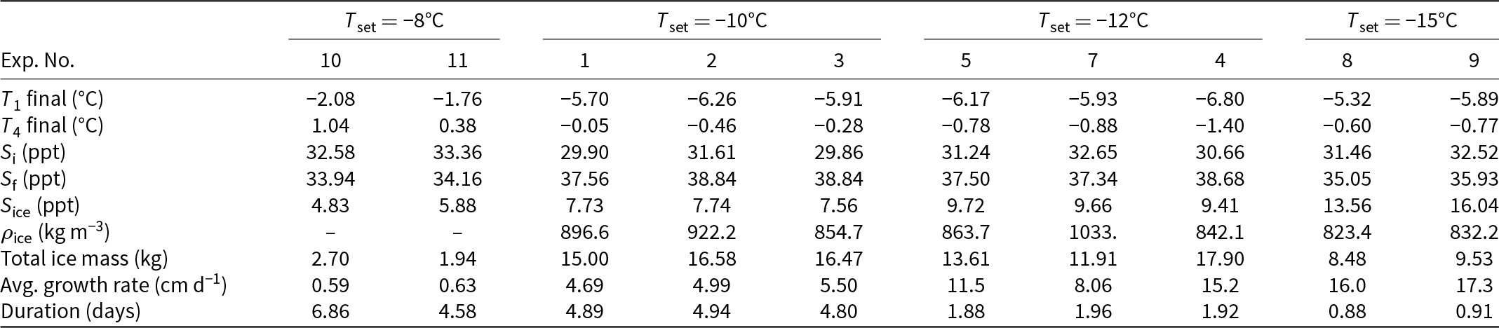
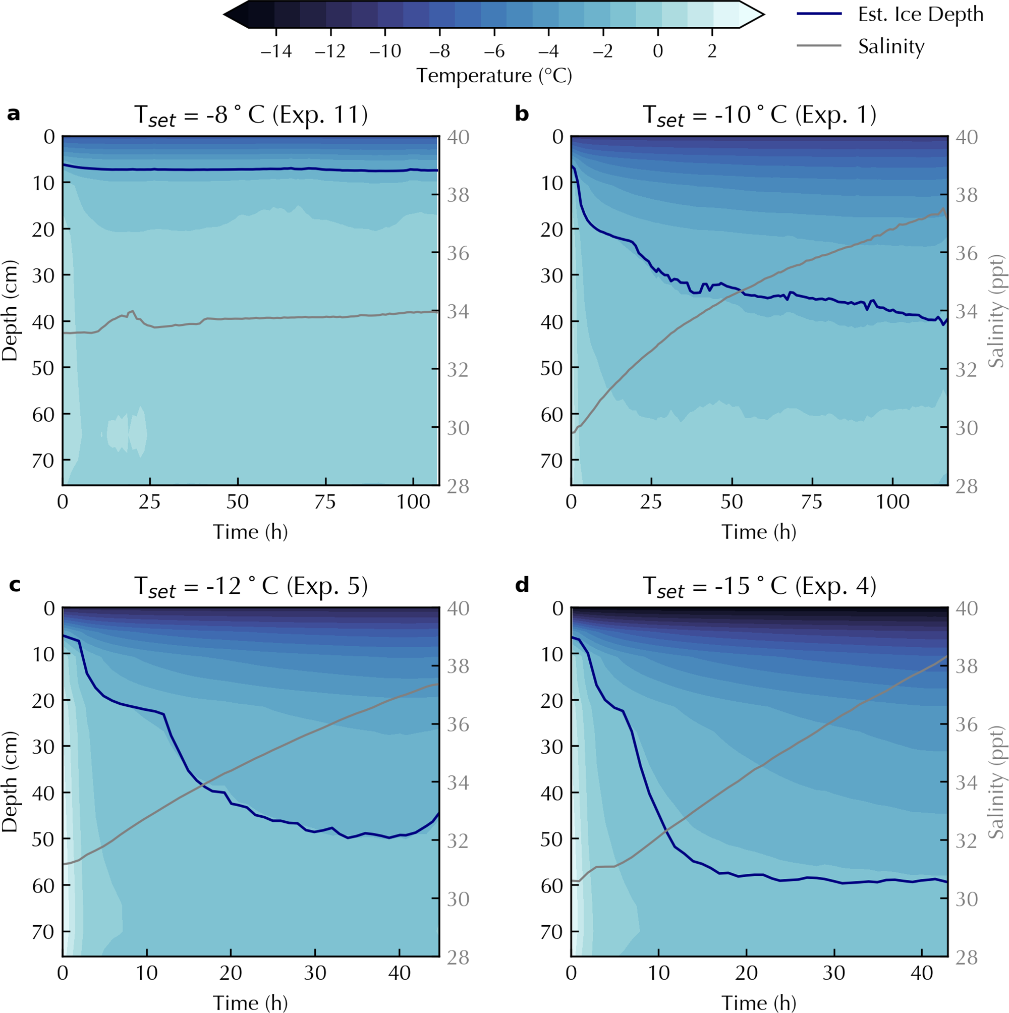
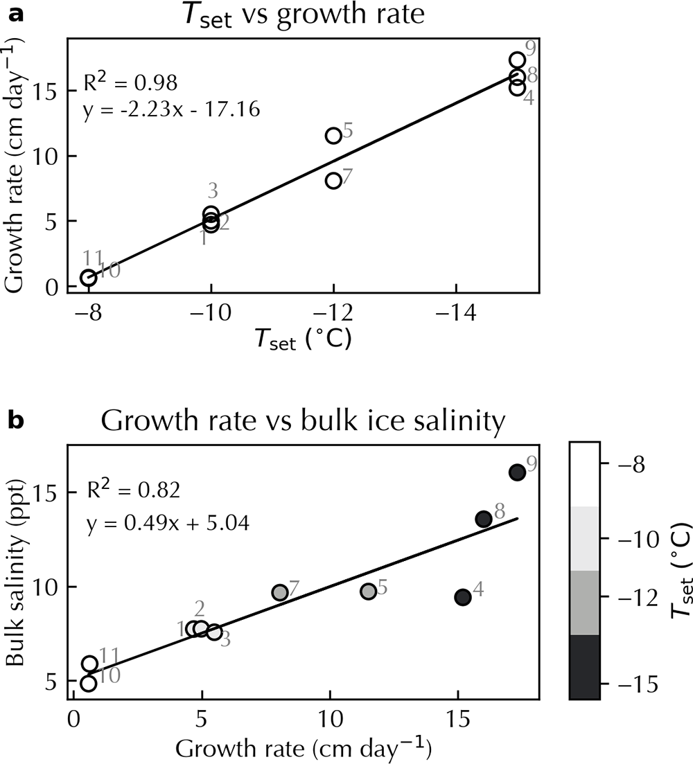
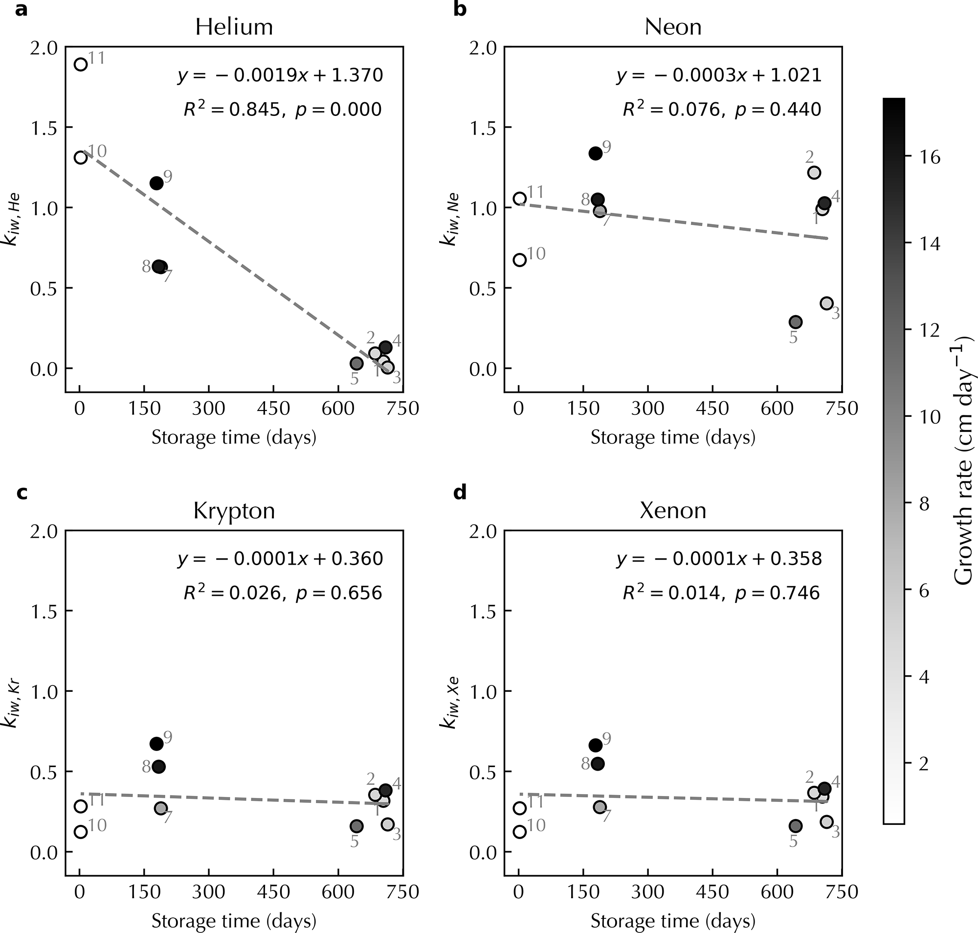
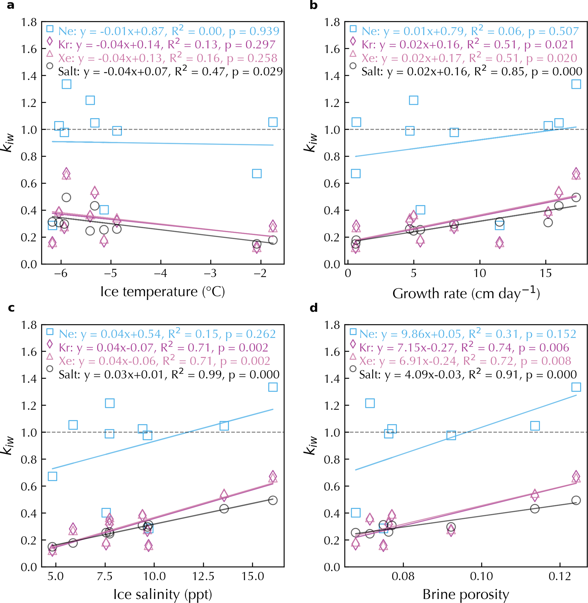
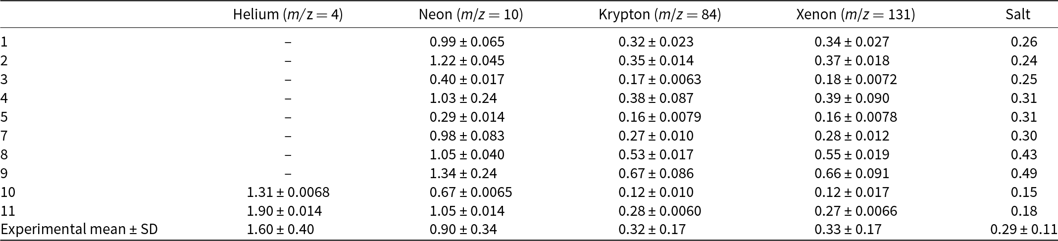
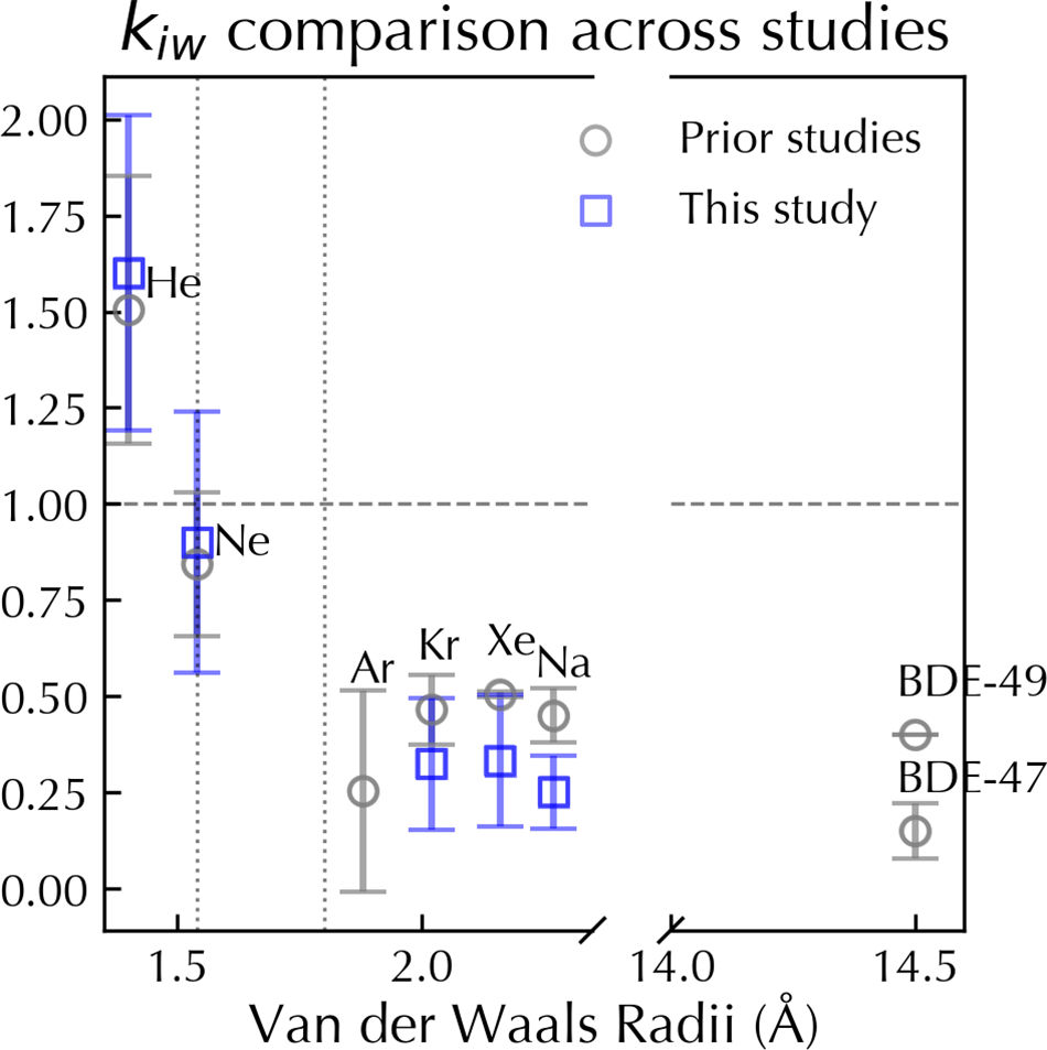
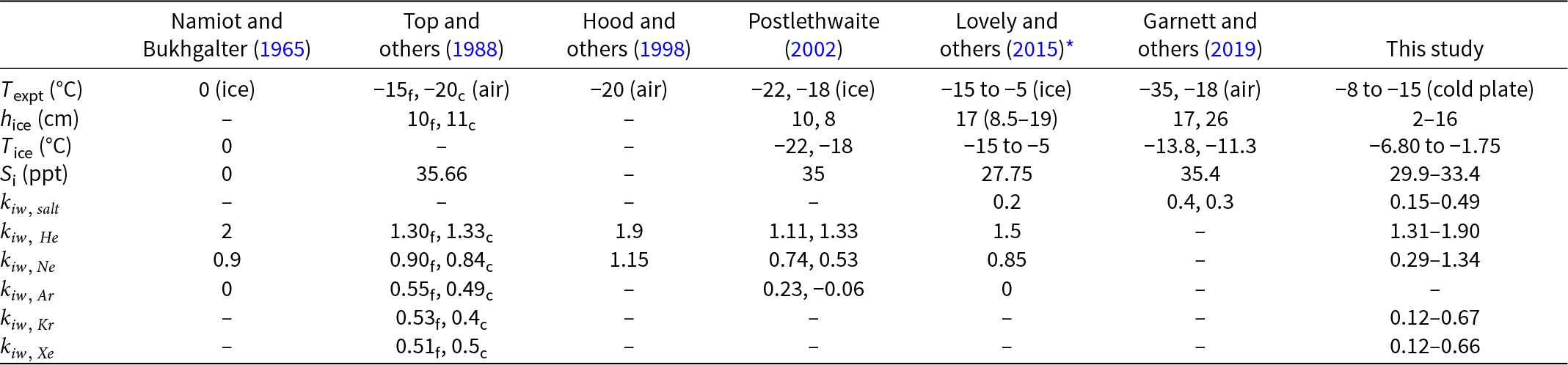
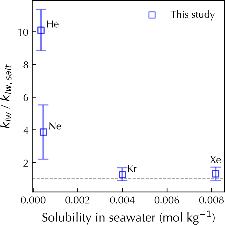


 Open access

