Introduction
Modern wireless communication systems increasingly require antennas capable of transmitting and receiving information across multiple frequency bands simultaneously. Multiple-input multiple-output (MIMO) antennas are widely adopted to meet these demands due to their ability to support high data rates and improve link reliability [Reference Salim, Singh, Dibs, Abed, Islam and Islam1–Reference Abed5]. However, one of the major challenges in MIMO systems is the mutual coupling that arises between closely spaced radiating elements, which can degrade overall system performance [Reference Abed5].
Several techniques have been proposed in the literature to enhance isolation and reduce mutual coupling, including: the use of slot structures between radiating elements [Reference Al, Singh and Abed6], spanner-shaped decoupling geometries [Reference Salim, Singh, Abed and Islam7], strip lines placed along the ground plane edges [Reference Abed8], electromagnetic bandgap (EBG) metamaterials [Reference Aparna, Ram and Kumar9], inserted metamaterial units [Reference Nahar, Rawat, Pathak, Kumar and Anguera10], T-shaped structures [Reference Jehangir and Sharawi11], and planar spiral-line decoupling networks [Reference Hussain and Sharawi12]. These methods aim to suppress surface currents or introduce counteracting fields that improve isolation in compact antenna arrays.
In MIMO and array antenna systems, the Total Active Reflection Coefficient (TARC) is an important parameter for assessing diversity performance, as it quantifies the ratio between the total outgoing (reflected) power and the total incident power across an N-port microwave component [Reference Abed5]. Although originally intended for multi-port structures, the active reflection coefficient concept can also be applied to individual radiating elements. Mathematically, TARC is defined as the square root of the sum of outgoing powers at all ports divided by the sum of all incident powers. Its value depends on excitation conditions such as scan angle and amplitude tapering, and it is also frequency-dependent. Therefore, TARC provides useful insight into how the radiation performance of a multi-port antenna varies across its operating bandwidth [Reference Abed5].
Table 1 summarizes important specifications reported in previous related works [Reference Al, Singh and Abed6–Reference Ding, Gao, Qu and Yin36], including the number of elements, Channel Capacity Loss (CCL), mutual coupling ( ${S_{ij}}$ isolation coefficient), efficiency, gain, physical size, and antenna type. These comparisons establish the performance context within which the proposed antenna is evaluated.
Comparison between previous antennas reported in [Reference Al, Singh and Abed6–Reference Ding, Gao, Qu and Yin36]

Table 1 Long description
The table compares various antennas based on elements, operating bandwidth, mutual coupling, efficiency, gain, size, and limitations. Most antennas have 2 to 4 elements, with bandwidths ranging from 0.95 GHz to 28.5 GHz. Mutual coupling is generally below -10 dB, indicating low interference between elements. Efficiency varies widely, with some antennas lacking reported data. Gain ranges from negative to positive values, with some antennas missing gain information. Many antennas are large and do not support key bands such as LTE, WLAN, and Wi-Fi 6, which are critical for modern communication systems. The table highlights the trade-offs between size, efficiency, and band support, suggesting that larger antennas often lack compatibility with essential frequency bands.
Design and experimental details
Antenna design
The fundamental geometry employed in this study is the butterfly ring, shown in Fig. 1, which represents the ground plate configuration originally proposed in [Reference Abed37]. The antenna was fabricated on an FR-4 substrate with a thickness of 0.8 mm, dielectric constant εr = 4.3, and loss tangent tan δ = 0.027 [Reference Abed37]. The overall dimensions of the baseline structure were 20 × 20 × 0.8 mm3 [Reference Abed37].
The fundamental butterfly ring [Reference Abed37].

Figure 1 Long description
The design includes a central circle with additional circles forming a butterfly-like shape. The outer boundary is bold, while the inner circles are dashed. Below the design, x and y axes are indicated with arrows pointing in their respective directions.
In the present work, the butterfly ring was miniaturized to one-fifth of its original size, resulting in a 4 × 4 × 0.8 mm3 element. This miniaturized butterfly ring is then used as the basis for a three-iteration fractal expansion. At the 0th iteration, the butterfly ring is rotated 45° clockwise to optimize space utilization for the higher-order iterations (Fig. 2). For each subsequent iteration, an additional butterfly ring is added, scaled to half the size of the ring used in the preceding step. This iterative process produces the compact multi-resonant “butterfly-flock” configuration used in the proposed antenna design.
Antenna configuration by four iterations.

Figure 2 Long description
The second panel labeled '1st Iter.' displays two butterfly rings stacked vertically. The third panel labeled '2nd Iter.' features three butterfly rings in a vertical arrangement. The fourth panel labeled '3rd Iter.' shows four butterfly rings stacked vertically, completing the sequence of iterations.
The transformation function R of the butterfly ring can be presented mathematically by Equation (1):
 \begin{equation}{R_i}\left[ {\begin{array}{*{20}{c}}
{{\text{ }}x} \\
{{\text{ }}y}
\end{array}} \right] = \left[ {\begin{array}{*{20}{c}}
{{\text{ }}r{\text{ }}cos\theta - s{\text{ }}cos\emptyset } \\
{r{\text{ }}sin\theta {\text{ }}s{\text{ }}sin\emptyset }
\end{array}} \right]\left[ {\begin{array}{*{20}{c}}
{{\text{ }}x} \\
{{\text{ }}y}
\end{array}} \right] + {\text{ }}\left[ {\begin{array}{*{20}{c}}
{{x_0}} \\
{{\text{ }}{y_0}}
\end{array}} \right]{\text{ }}\end{equation}
Where r and s are the reduction scale, which are equals to 0.5,  $\theta $ and
 $\emptyset $ are the rotation angles,
 $\theta $ equals to while
 $\emptyset $ equals to
 ${0^0}$ (no rotation in H-Plane).
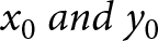 ${x_0}{\text{ }}and{\text{ }}{y_0}$ are the amounts of translation, the translation in Y-direction only, therefore,
 ${x_0}$ equals to zero and the value of
 ${y_0}$ depends on the order of iteration. Therefore, equation (1) can be simplified to:
 \begin{equation}{R_i}\left[ {\begin{array}{*{20}{c}}
{{\text{ }}x} \\
{{\text{ }}y}
\end{array}} \right] = \left[ {\begin{array}{*{20}{c}}
{{\text{ }}0 - 0.5} \\
{0.5{\text{ }}0{\text{ }}}
\end{array}} \right]\left[ {\begin{array}{*{20}{c}}
{{\text{ }}x} \\
{{\text{ }}y}
\end{array}} \right] + {\text{ }}\left[ {\begin{array}{*{20}{c}}
0 \\
{{\text{ }}{y_0}}
\end{array}} \right]{\text{ = }}\,\left[ {\begin{array}{*{20}{c}}
{ - 0.5x} \\
{0.5{\text{ }}y + {y_0}}
\end{array}} \right]\end{equation}
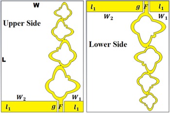
The proposed antenna consists of dual symmetrical radiation elements, each radiating element located at another side of the substrate to reduce the mutual coupling (Fig. 3). Each antenna consists of a flock of butterfly rings, which are configured in three iterations. The dual radiating elements fed by CPW contains of feeding strip line F with dimensions of (1.5 mm × 4.5 mm) sectioned from miniaturized ground by a hole g of 0.5 mm, the ground consists of two parts, small part with dimensions of  ${l_1}$ ×
 ${W_1}$ = 4 mm × 7 mm and large part with dimensions of
 ${l_1}$ ×
 ${W_2}$ = 4 mm × 20.5 mm as it is shown in Fig. 3.
The proposed butterflied flock MIMO antenna.

Figure 3 Long description
The diagram consists of two parts labeled 'Upper Side' and 'Lower Side'. The lower side also displays butterfly rings, with dimensions labeled as l subscript 1, W subscript 2, W subscript 1, g and F. The elements are positioned on either side of the substrate to reduce mutual coupling. The feeding strip line F is sectioned from the miniaturized ground by a hole labeled g. The ground consists of two parts: a small part with dimensions l subscript 1 times W subscript 1 equals 4 millimeters times 7 millimeters and a large part with dimensions l subscript 1 times W subscript 2 equals 4 millimeters times 20.5 millimeters.
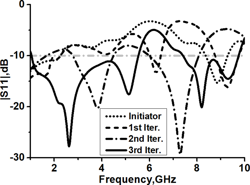
Figure 4 shows the dual operating band represented by the dotted curve of 1–2.3 GHz and 8.3–9.3 GHz for the antenna. At the 1st iteration, triple operating band observed at 1–2.3 GHz, 6–6.5 GHz and 8.7–9.7 GHz (the dashed curve in Fig. 4), while at the 2nd iteration, dual band observed at 2.6–4.8 GHz and 6–8 GHz (the dotted dashed curve in Fig. 4). An additional butterfly structure in the 3rd iteration produces dual wide operating bands of 1.1–5.6 GHz and 7.4–9.7 GHz (illustrated in Fig. 4 as solid curve) which can contribute many wireless communications like: GPS (1.272 GHz/1.575), 3G (1.8 GHz/1.9 GHz), WLAN (2.4 GHz/5 GHz), LTE (2.6 GHz/3.5 GHz and 5 GHz), Wi-Fi6, ISM (Industrial, Scientific and Medical) and mobile satellite communications (7–9 GHz). The overall size of the Butterflies Flock MIMO Fractal Antenna is 30 × 40 × 0.8 mm3.
Simulated S11 at all iterations.

Figure 4 Long description
The x-axis is labeled 'Frequency, GHz' ranging from 1 to 10 and the y-axis is labeled '|S11|, dB' ranging from -30 to 0. Four curves are plotted: a dotted line for the initiator, a dashed line for the first iteration, a dash-dotted line for the second iteration and a solid line for the third iteration. Each curve shows different frequency responses across the range, with varying peaks and troughs indicating different operating bands for each iteration.
Diversity performance
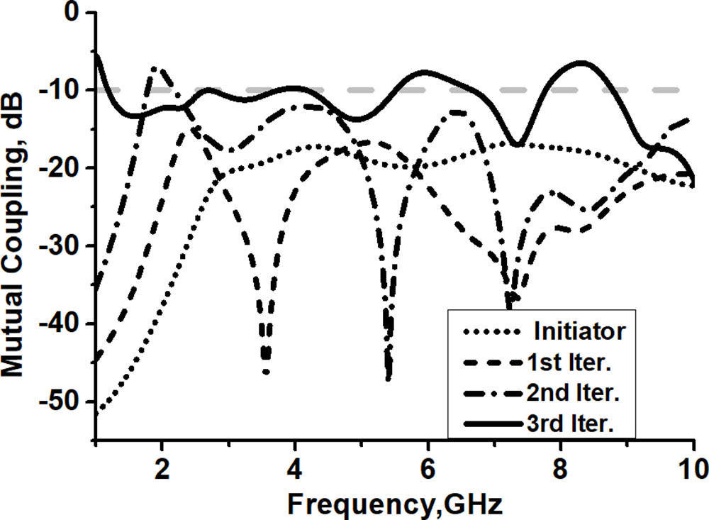
The mutual coupling between the dual radiating elements is down (−50  $\sim$ −15 dB) at 0th iteration, as shown in Fig. 5 (the dotted curve). An additional butterfly structure at high order iteration cause increment in the length of the radiating elements which lead to reduce the distance separated between the dual antennas than to increase the amounts of mutual coupling over the process of MIMO antenna configuration (Fig. 5). In addition, the amounts of mutual coupling between the dual antennas are less than −10 dB during the operating bands of 1.1–5.6 GHz and 7.4–9.7 GHz in the 3rd iteration as it is shown in Fig. 5 (the solid curve).
Simulated mutual coupling at all iterations.

Figure 5 Long description
The graph shows mutual coupling in decibels on the y-axis versus frequency in gigahertz on the x-axis, ranging from 0 to 10 GHz. Four curves represent different iterations: initiator, 1st iteration, 2nd iteration and 3rd iteration. The initiator curve is solid, the 1st iteration is dashed, the 2nd iteration is dotted and the 3rd iteration is dash-dotted. The mutual coupling values vary across the frequency range, with peaks and troughs visible for each curve. The legend identifies each curve by its iteration type.
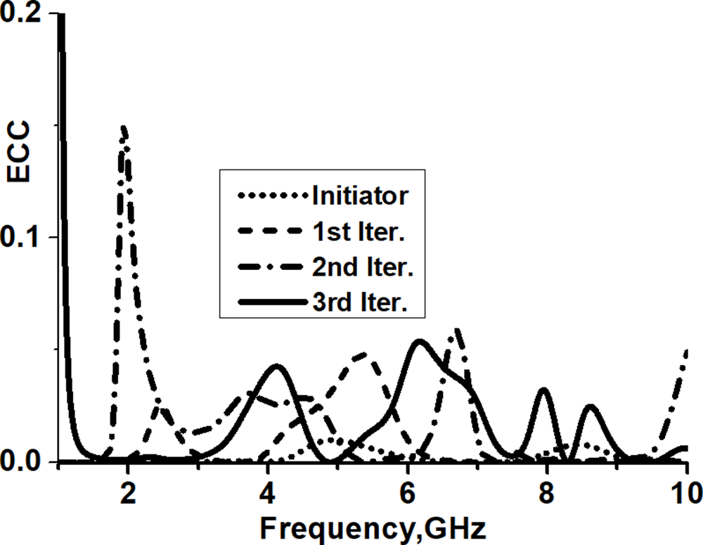
The envelope correlation coefficient (ECC) is used to investigate the antenna diversity. The ECC is calculated by using the values of the S-parameters according to equation (3) [Reference Abed5]. Figure 6 shows low values of ECC at all iterations (ECC must be  $ \lt $0.5), the lower values of ECC indicate that there is diversity between radiating elements due to the proposed MIMO. The above study matches the values of mutual coupling in Fig. 5.
 \begin{equation}{\text{ECC = }}\frac{{{{\left| {S_{11}^*{S_{12}} + S_{21}^*{S_{22}}} \right|}^2}}}{{\left( {1 - {{\left| {{S_{11}}} \right|}^2} - {{\left| {{S_{21}}} \right|}^2}} \right)\left( {1 - {{\left| {{S_{22}}} \right|}^2} - {{\left| {{S_{12}}} \right|}^2}} \right)}}\end{equation}
Simulated ECC at all iterations.

Figure 6 Long description
The x-axis is labeled 'Frequency, GHz' ranging from 0 to 10 and the y-axis is labeled 'ECC' ranging from 0.0 to 0.2. Four curves are depicted: Initiator (dotted line), 1st Iteration (dashed line), 2nd Iteration (dash-dot line) and 3rd Iteration (solid line). The graph illustrates variations in ECC values across different frequencies for each iteration.
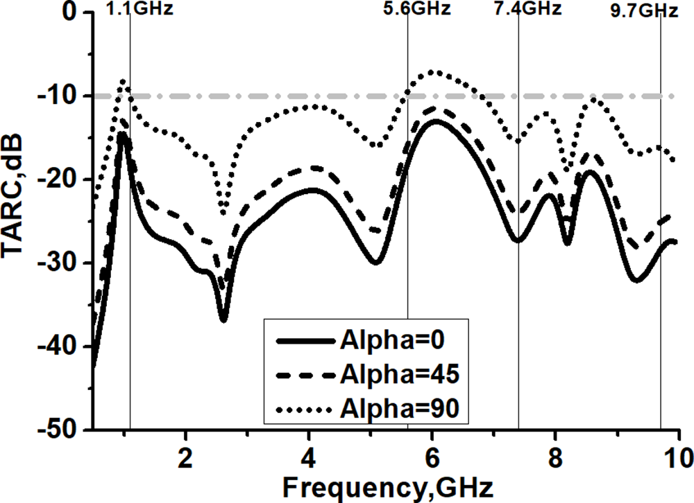
The TARC values for incident angle  ${\alpha }$ equals to
 ${\text{ }}0$,
 $45$, and
 $90{\text{ degrees}}$ is illustrated in Fig. 7, which are calculated according to Equation (4) [Reference Abed5]. The solid curve in Fig. 7 indicates that the antenna has high isolation between the radiating elements during operating bands when
 ${\alpha } = 0{\text{ degree}}$ wherein TARC values vary from −15 dB to −35 dB at lower band (1.1–5.6 GHz) and vary between −20 dB and −35 dB at the upper band (7.4–9.7 GHz).
 \begin{equation}{\text{TARC}} = {\text{ }}\frac{{\sqrt {(\left| {\left( {{{\mathbf{S}}_{11}} + {\text{ }}{{\mathbf{S}}_{12}}{{\mathbf{e}}^{{\mathbf{j}}\alpha }}} \right){|^2} + } \right|\left( {{{\mathbf{S}}_{21}} + {\text{ }}{{\mathbf{S}}_{22}}{{\mathbf{e}}^{{\mathbf{j}}\alpha }}){|^2}} \right)} }}{{\sqrt 2 }}\end{equation}
Even when ${\,\alpha }$ =
 $90{\text{ degrees}}$, the values of TARC during the dual operating band of the proposed antenna still
 $ \lt $−10 dB. That happened due to the location of the radiating elements on opposite face of the substrate.
Simulated TARC when  ${\alpha }\,{\text{ = 0}}$, 45, and 90 degrees for the 3rd iteration.

Figure 7 Long description
A graph showing the total active reflection coefficient (TARC) in decibels on the y-axis versus frequency in gigahertz on the x-axis. The graph includes three curves representing different incident angles: a solid line for 0 degrees, a dashed line for 45 degrees and a dotted line for 90 degrees. The frequency range is from 1 to 10 gigahertz, with notable points at 1.1, 5.6, 7.4 and 9.7 gigahertz. The TARC values range from 0 to negative 50 decibels.
Surface current distribution
Figure 8 illustrates the surface current distribution at the resonant frequencies of 1.575, 2.6, 5, and 8 GHz. At 1.575 GHz, the current flows predominantly along the feeding line F, the 1st butterfly, the 2nd butterfly, and approximately half of the 3rd butterfly. The effective current path length is 28 mm, which corresponds to roughly 1/8 of the wavelength at this resonant frequency, confirming the formation of a lower-order resonance mode.
Surface current at 1.575, 2.6, 5, and 8 GHz.

Figure 8 Long description
The image shows four panels illustrating surface current distribution at different resonant frequencies: 1.575 GHz, 2.6 GHz, 5 GHz and 8 GHz. Each panel displays a structure with labeled sections: 'Init.', '1st', '2nd' and '3rd'. A color scale on the right indicates current intensity, ranging from 0 to 120. The current distribution varies across the frequencies, with distinct patterns visible in each panel.
At 2.6 GHz, the current is mainly concentrated along the 1st and 2nd butterfly rings, yielding a total path length of 24 mm, which is close to λ/4 at 2.6 GHz. As the operating frequency increases (5 and 8 GHz), the surface current density becomes more confined to shorter paths on the radiator. This corresponds to higher-order resonances where the effective electrical lengths approach λ/2 and λ, enabling strong current confinement and efficient radiation at higher frequencies.
Beyond simple geometric scaling, the 45° clockwise and counter-clockwise rotations of the butterfly rings in successive iterations introduce nonlinear current routing, effectively increasing the electrical path while preserving compact physical size. This rotational fractal behavior not only saves physical area but also creates extended meandering current trajectories, enabling the antenna to support resonant modes in the lower band (1.1–5.6 GHz) despite its miniaturized structure. Consequently, by the 3rd iteration, the antenna exhibits the multi-resonant characteristics required for wide dual-band operation.
Channel capacity loss
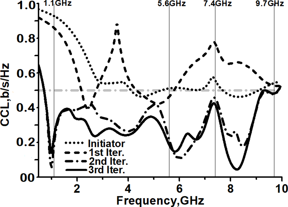
CCL values are reduced during the progress of the proposed MIMO configuration, as shown in Fig. 9. For the initiator antenna (the dotted curve) as well as the 1st iteration (the dashed curve), the values of CCL are larger than the critical value (0.5 b/s/Hz), especially at lower operating band.
Simulated CCL at all iterations.

Figure 9 Long description
Four curves represent the initiator and three iterations. The initiator curve is dotted, the first iteration is dashed, the second iteration is dash-dotted and the third iteration is solid. Peaks and troughs are visible across the frequency range from 1 to 10 gigahertz, with notable points at 1.1, 5.8, 7.4 and 9.7 gigahertz.
The CCL characterizes the quality of the MIMO system, which can be calculated according to equation (5) [Reference Deng, Li, Zhao and Guo17]:
 \begin{equation}CCL = - 10lo{g_2}{\text{ }}det\left( \rho \right)\end{equation}
Where  $\rho $ is the correlation matrix of receiving antenna and can be calculated as:
 \begin{align*}
\rho &= \left[\begin{array}{@{}l@{\quad}l@{}}
{{\rho _{11}}} & {{\rho _{12}}} \\
{{\rho _{21}}} & {{\rho _{22}}}\end{array} \right]\!,\quad {\rho _{ii}}= 1-({|s_{ii}|}^2 + {|s_{ij}|}^2) \quad\text{and } \\
{\rho _{ij}} &= {({s_{ii}}{\text{ }}{s_{ij}}{\text{ }})^2} + {({s_{ji}}{\text{ }}{s_{ij}}{\text{ }})^2},
\, i,j = 1 \text{ or }2\end{align*}
Acceptable values of CCL ( $ \lt $ 0.5) are observed in Fig. 9 at the 2nd iteration (the dashed dotted curve) and the 3rd iteration (the solid curve). The quality of the system is improved (low CCL) at the 2nd and the 3rd iteration due to the reduction of the correlation matrix value of receiving antenna
 $\rho $ in Equation (5) [Reference Abed5].
Results and discussions
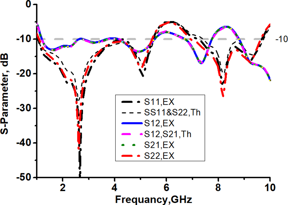
Figure 10 shows the prototype of the butterfly’s flock MIMO fractal antenna, while Fig. 11 depicts the measured and simulated values of the reflection coefficients.
Prototype photographs. (a) The upper side. (b) The lower side.

Figure 10 Long description
It features a series of fractal patterns on a rectangular board with a connector at the top and bottom. A paper clip is positioned to the left of the board. The image B shows the lower side of the same antenna prototype. Similar fractal patterns are visible, with connectors at the top and bottom. A paper clip is positioned to the left of the board, similar to the first image.
Simulated and measured radiation patterns.

Figure 11 Long description
The graph shows S-parameters in decibels plotted against frequency in gigahertz. The x-axis is labeled 'Frequency, GHz' and the y-axis is labeled 'S-parameter, dB'. Multiple curves are present: S11.EX (dashed line), SS11&S22,Th (solid line), S12,EX (solid line), S12,S21,Th (solid line), S21.EX (dotted line) and S22.EX (solid line). The curves display various peaks and troughs across the frequency range from 0 to 10 GHz, with values ranging from -50 dB to -10 dB. Each curve represents different measured and simulated values of reflection coefficients, showing distinct patterns and intersections at various frequencies.
Figure 11 shows a good agreement between the measured and simulated radiation patterns. The radiation patterns in H-plane (the dashed red curves) that have been measured within all resonant frequencies are around omnidirectional, whereas in E-Plane, at higher frequencies, the radiation pattern becomes directional, as shown in Fig. 12.
Simulated and measured radiation patterns. (a) 2.6 GHz. (b) 5 GHz. (c) 7.7 GHz. (d) 9.4 GHz.

Figure 12 Long description
The simulated curves are shown in black for the E-plane and green for the H-plane, while the measured curves are shown in red for the E-plane and blue for the H-plane. The plots illustrate the directional characteristics of the radiation patterns at each frequency, with variations in shape and directionality across the different frequencies.
Figure 12 presents the normalized radiation patterns at resonant frequencies of 2.6, 5, 7.7, and 9.4 GHz. An acceptable agreement was attained between the simulated (solid curves) and measured (dashed curves) radiation patterns in the E-plane (black curves) and H-plane (red curves). The measured radiation pattern in the E plane at 2.6 GHz has two lobes at angles of 1100 and 300° (Fig. 12(c), the black dashed curve).
Figure 12(d) shows an apple shape, which presents the measured radiation pattern in the E plane at the frequency of 9.4 GHz; the pattern is null at 300°. The directivity D increases with increasing frequency (reducing the wavelength λ), as shown by equation (6).
 \begin{equation}{\text{D }} = {\text{ }}\frac{{4{\text{ }}\pi {\text{ }}{A_e}}}{{{\lambda ^2}}}\end{equation}
Fig.13(a) illustrates the measured values of the gain (the blue curve) and efficiency (the black curve). It is clear that the values of the gain 0.5–4.8 dB and the efficiency of the proposed antenna varied from 60% to 85%. Fig. 13(b) shows the radiation measuring chamber used for the data collection.
(a) Measured gain and efficiency. (b) Measurements chamber.

Figure 13 Long description
The efficiency curve, marked with squares, starts at 60 percent and rises to 85 percent across the frequency range of 1 to 10 gigahertz. The gain curve, marked with circles, starts at 0.5 decibels and increases to 4.8 decibels over the same frequency range. The image B shows a radiation measuring chamber with a tripod-mounted device and a panel with attached equipment. The chamber walls are covered with material designed to absorb radio waves and the setup is used for data collection related to antenna measurements.
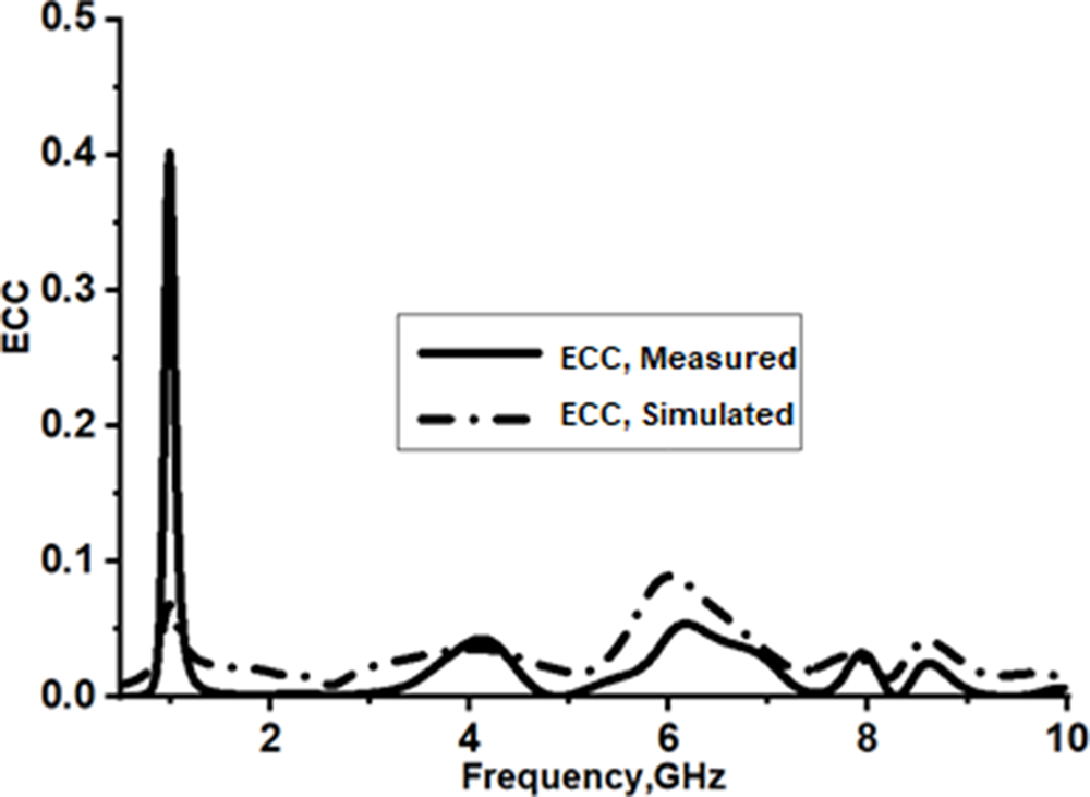
Figure 14 illustrates the measured (the solid curve) and simulated (the dashed-doted curve) values of ECC. It is clear that the butterfly flock MIMO antenna had lower values of ECC for all bands (< 0.5).
Measured and simulated values of ECC.

Figure 14 Long description
The y-axis is labeled 'ECC' ranging from 0 to 0.5. The solid curve represents measured ECC values, while the dashed dotted curve represents simulated ECC values. Both curves show variations across the frequency range, with peaks and troughs visible at different points.
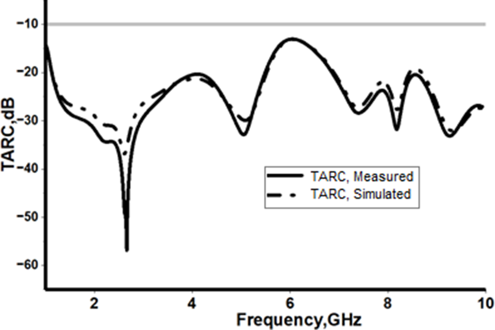
The TARC values vary from −15 dB to −35 dB (measured and simulated) at Fig. 15 indicated that the proposed antenna has low TARC at incident angle of 0 degrees.
Measured and simulated values of TARC (0 degrees).

Figure 15 Long description
The graph shows the total active reflection coefficient (TARC) values plotted against frequency in gigahertz (GHz), ranging from 2 to 10 GHz. The y-axis is labeled as TARC in decibels (dB) and the x-axis is labeled as Frequency in gigahertz (GHz). Two curves are present: one solid line representing measured TARC values and one dashed line representing simulated TARC values. The measured values show a significant dip around 3 GHz, reaching below minus 50 dB, while the simulated values follow a similar trend but with less pronounced dips. Both curves exhibit multiple peaks and troughs across the frequency range.
Table 2 shows a comparison between the proposed antenna with 18 previous works, which have 2 radiation elements, based on important properties such as operating band, mutual coupling, efficiency, gain, and size.
Comparison between previous antennas and the proposed antenna
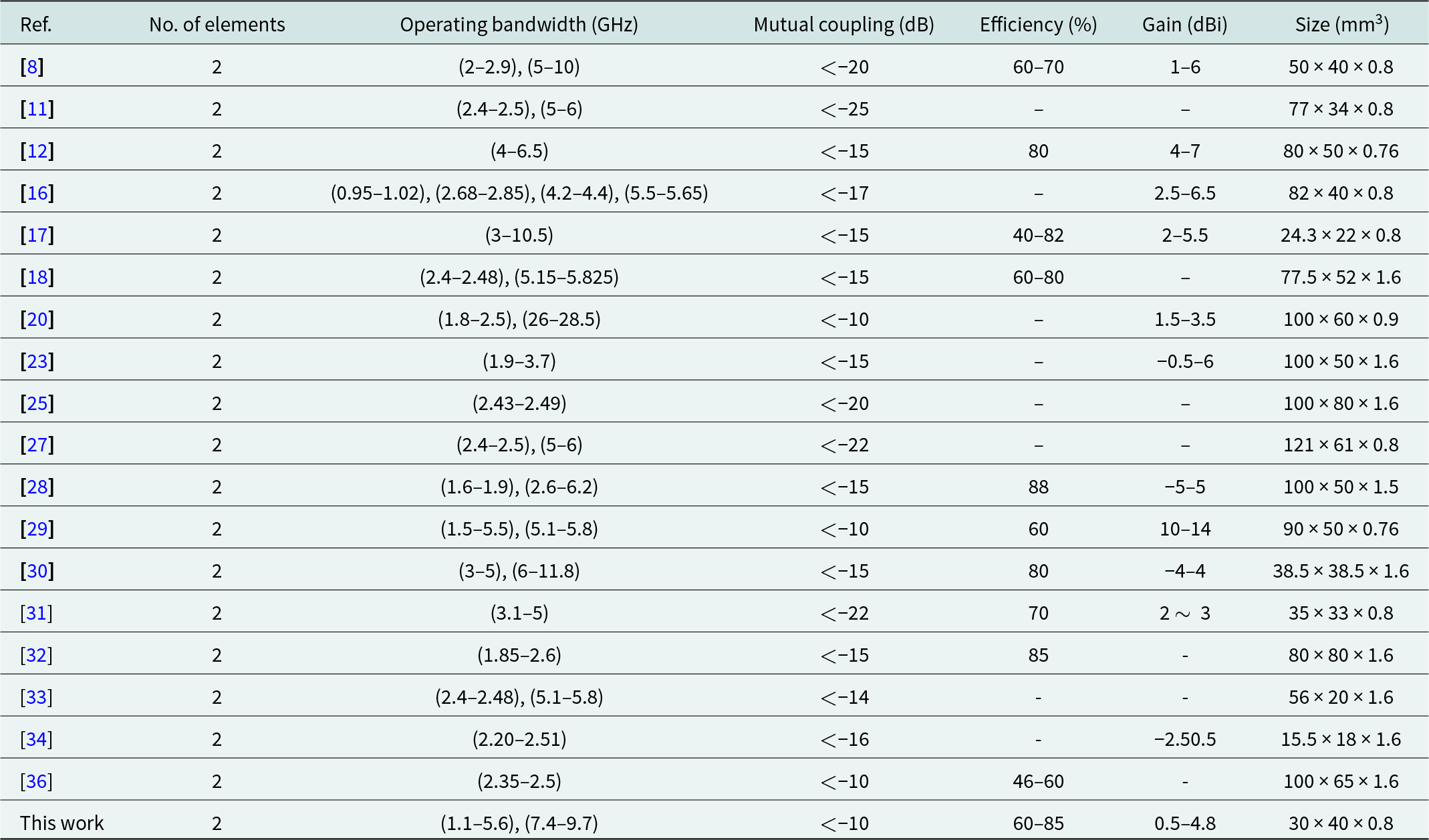
Table 2 Long description
The table compares various antennas based on the number of elements, operating bandwidth, mutual coupling, efficiency, gain, and size. The proposed antenna stands out with a wide operating bandwidth of 1.1-5.6 GHz and 7.4-9.7 GHz, maintaining mutual coupling below -10 dB. It achieves an efficiency range of 60-85% and a gain between 0.5 and 4.8 dBi, all within a compact size of 30 x 40 x 0.8 mm3. In comparison, other antennas show varied bandwidths and efficiencies, with some lacking data on efficiency and gain. The proposed antenna's compact size and performance metrics suggest a balance between size and functionality, making it a competitive option among the listed antennas.
Table 2 presents the key performance metrics of the proposed butterfly-flock MIMO fractal antenna, consolidating the results from the simulated and measured analyses. The table highlights several important contributions of this work. First, the antenna achieves wide dual-band operation across 1.1–5.6 GHz and 7.4–9.7 GHz, demonstrating that the iterative butterfly-ring geometry and its rotational fractal progression successfully generate multiple resonant modes required for modern multiband systems. This validates the effectiveness of the miniaturized ring iterations in producing extended meandered current paths while maintaining a compact footprint.
Table 2 also shows low mutual coupling between antenna elements, indicated by the isolation values S₁₂/S₂₁, which remain below acceptable limits across both bands. This performance is achieved without external decoupling structures, a significant contribution enabled by the anti-phase rotational placement of the butterfly iterations on opposite faces of the substrate. This inherent spatial polarization diversity reduces surface-wave interaction and makes the design simpler and more integrable than approaches using EBGs, DGS, or neutralization lines.
Furthermore, the diversity performance parameters, including the ECC, TARC, and CCL, indicate that the proposed antenna maintains stable orthogonality and efficient signal diversity across both operating bands. The ECC values remain well below the 0.5 threshold, while the low TARC values confirm that the geometry yields minimal reflected power under multi-port excitation. Likewise, the CCL values demonstrate that the antenna supports reliable data throughput with minimal capacity degradation, validating the suitability of the structure for high-data-rate MIMO applications.
Finally, the radiation efficiency, realized gain, and compact size (30 × 40 × 0.8 mm3) collectively underline the practical advantage of the design for portable and space-constrained wireless devices. The performance metrics in Table 2 confirm that the proposed butterfly-flock configuration not only achieves multiband operation but also offers enhanced isolation and diversity characteristics that are technically superior to earlier fractal or compact MIMO antennas.
Conclusion
The proposed Butterflies Flock MIMO Fractal Antenna demonstrates significant advancements over previously reported designs. It achieves dual wide operating bands (1.1–5.6 GHz and 7.4–9.7 GHz), enabling support for multiple wireless standards, including RFID, LTE, Wi-Fi 6, ISM, GPS, WLAN, and satellite communications. The antenna combines compact dimensions (30 × 40 × 0.8 mm3) with high efficiency (60–85%), acceptable gain (0.5–4.8 dBi), and low mutual coupling (<−10 dB), ensuring robust isolation and diversity performance as reflected by ECC < 0.5 and minimal CCL. The novel fractal configuration, based on iterative miniaturization and rotation of butterfly rings, enhances bandwidth while maintaining a low-profile structure. These features collectively position the design as an efficient and versatile solution for next-generation portable and high-data-rate communication systems.
Acknowledgement
Appreciation to the Universiti Sains Malaysia (USM) and AlShaab University, Baghdad, Iraq, for these collaborations. This research is supported by the Malaysian Ministry of Higher Education under the Fundamental Research Grant Scheme (project code: FRGS/1/2025/TK07/USM/01/1).
Competing interests
The authors declare none.

Amer T. Abed received the B.Sc. Degree in electrical engineering from the College of Engineering, University of Baghdad, in 1984, the master’s degree in communication engineering from the University of Tenaga, Malaysia, and the Ph.D. degree from the National University of Malaysia. He is currently Assist. Professor and Chairman of Artificial Intelligence Engineering, College of engineering and information Technology, AlShaab University, Baghdad, Iraq. He has wide experience in designing the RF circuit and antenna field. He has published 25 articles in ISI journals and two books about antenna design. He is a member of the European Microwave Association (EMA). He has reviewed more than 40 articles in the IET and the IEEE journals.

Widad Ismail received the B.Eng. (H) degree in electronics and communication engineering from the University of Huddersfield, United Kingdom, in 1999, and the Ph.D. degree in electronics and communication engineering from the University of Birmingham, United Kingdom, in 2004. Her main areas of research are wireless system design, radio frequency identification, active integrated antennas, and wireless and microwave systems engineering. She is currently a Lecturer and Project Coordinator for the Auto-ID Laboratory (AIDL), Universiti Sains Malaysia. She is also a Member of the Institute of Electrical and Electronics Engineers, the Wireless World Research Forum (WWRF), and a Professional Engineer under the Board of Engineers Malaysia.

Hadi Jameel Hadi received the B.Sc. degree from the Department of Electrical Engineering, Al Mustansiriya University, Iraq, in 2010, and the M.Sc. degree in electronic and communication engineering from Al Mustansiriya University, Iraq, in 2013. From 2013 to 2018, he was a University Teacher and Researcher. Since 2018, he has been a Professional Staff Member at Oil Products Distribution Company (OPDC). He has a strong interest in research development and the publication process. He is the author of eight papers. His research interests include antennas, wireless communications, radar, and wireless sensor networks.