1 Introduction
Palaeomagnetic data have shown that the Earth’s magnetic field has existed for more than three billion years (e.g. Tarduno et al.
Reference Tarduno, Cottrell, Davis and Nimmo2015). Thermocompositional convection is the primary driver of the dynamo generation processes that occur in Earth’s liquid metal core (Buffett et al.
Reference Buffett, Huppert, Lister and Woods1996; Roberts & King Reference Roberts and King2013). Prior to the
 $O(1)$
Ga nucleation of the solid inner core, most evolution models find that thermally buoyant anomalies drove core convection, whereas a compositionally fuelled core flow has dominated since the formation of the inner core (e.g. Buffett et al.
Reference Buffett, Huppert, Lister and Woods1996; Davies et al.
Reference Davies, Pozzo, Gubbins and Alfé2015, contrasted with O’Rourke & Stevenson Reference O’Rourke and Stevenson2016; Huguet et al.
Reference Huguet, Van Orman, Hauck and Willard2018). However, the detailed dynamics of convective flows in planetary core-like liquid metals still remains largely unexplored (see Calkins et al.
Reference Calkins, Aurnou, Eldredge and Julien2012; Guervilly & Cardin Reference Guervilly and Cardin2016; Kaplan et al.
Reference Kaplan, Schaeffer, Vidal and Cardin2017).
This laboratory experimental investigation focuses on thermally driven, rotating convection of the liquid metal gallium in a cylindrical tank. The characterisation of these flows is a necessary step towards understanding the larger problem of thermocompositionally driven, turbulent convection, which fuels the dynamo in Earth’s outer core. Such rotationally dominated convective flows underlie quasigeostrophic dynamo action (e.g. Calkins et al. Reference Calkins, Julien, Tobias and Aurnou2015; Nataf & Schaeffer Reference Nataf and Schaeffer2015; Calkins Reference Calkins2017), as likely occurs in a number of solar system planetary dynamos and in the majority of present-day numerical dynamo models (e.g. Soderlund et al. Reference Soderlund, Sheyko, King and Aurnou2015; Yadav et al. Reference Yadav, Gastine, Christensen, Wolk and Poppenhaeger2016a ; Aurnou & King Reference Aurnou and King2017; Schaeffer et al. Reference Schaeffer, Jault, Nataf and Fournier2017). Furthermore, this study lays a quantitative foundation for understanding the changes that arise in the largely unexplored magnetostrophic regime (e.g. Roberts & King Reference Roberts and King2013; King & Aurnou Reference King and Aurnou2015; Yadav et al. Reference Yadav, Gastine, Christensen, Wolk and Poppenhaeger2016a ,Reference Yadav, Gastine, Christensen, Duarte and Reiners b ).
With gravity parallel to both the rotation axis and the axis of the cylindrical container, the experimental set-up employed here, in particular, simulates convective processes occurring at high latitudes within a planetary core’s tangent cylinder volume (Aurnou et al.
Reference Aurnou, Andreadis, Zhu and Olson2003; Aujogue et al.
Reference Aujogue, Pothérat, Sreenivasan and Debray2018). In rapidly rotating spherical shells that approximate a planet’s outer core geometry, thermal convection onsets outside the tangent cylinder (Busse Reference Busse1970) or via equatorially trapped thermal inertial waves (Zhang & Schubert Reference Zhang and Schubert2000). The high-latitude regions inside the tangent cylinder start to convect only at significantly higher supercriticalities. However, precisely when convection within the tangent cylinder commences cannot be inferred from linear stability results, since typical convective flows outside the tangent cylinder are already governed by strongly nonlinear dynamics at this point. It is clear, though, that the polar and equatorial regions differ fundamentally with regard to their convective flow structures (Glatzmaier & Roberts Reference Glatzmaier and Roberts1995; Simitev & Busse Reference Simitev and Busse2005; Sreenivasan & Jones Reference Sreenivasan and Jones2006; Aubert, Aurnou & Wicht Reference Aubert, Aurnou and Wicht2008) and heat transport properties (Busse & Simitev Reference Busse and Simitev2006; Aurnou et al.
Reference Aurnou, Heimpel, Allen, King and Wicht2008; Yadav et al.
Reference Yadav, Gastine, Christensen, Duarte and Reiners2016b
). These differences persist in fully turbulent convection cases where tangent cylinder flows appear to be dominant contributors to the global dynamo action, both in the earliest dynamo models and in the highest-resolution models carried out to date (Glatzmaier & Roberts Reference Glatzmaier and Roberts1995; Schaeffer et al.
Reference Schaeffer, Jault, Nataf and Fournier2017). High-latitude planetary core flows are likely, then, to be important for understanding planetary-scale dynamo generation processes, and our low-
 $Pr$
, tangent cylinder-like convection experiments provide insight into the behaviours of such flows.
The paper is organised as follows. In § 2, we present the dimensionless parameters that characterise the rotating Rayleigh–Bénard convection system as well as the basic scaling results for the threshold of the convective instability. In § 3, we present our laboratory set-up and the material properties of liquid gallium. The laboratory experimental results are given in § 4. Finally, in § 5, comparisons are made between the novel liquid metal rotating convective flows found here and the non-metallic rotating convective flows. In addition, we extrapolate our results to more extreme planetary core settings.
2 Parameter definitions and scaling predictions
2.1 Non-dimensional parameters
The control parameters in thermal convection systems are most meaningfully expressed in terms of characteristic time scales (e.g. Cheng & Aurnou Reference Cheng and Aurnou2016). The molecular properties of the fluid are non-dimensionally characterised by the thermal Prandtl number:
 $$\begin{eqnarray}\displaystyle & \displaystyle Pr={\displaystyle \frac{\unicode[STIX]{x1D70F}_{\unicode[STIX]{x1D705}}}{\unicode[STIX]{x1D70F}_{\unicode[STIX]{x1D708}}}}={\displaystyle \frac{\unicode[STIX]{x1D708}}{\unicode[STIX]{x1D705}}}. & \displaystyle\end{eqnarray}$$
This is the ratio of the thermal diffusion time
 $\unicode[STIX]{x1D70F}_{\unicode[STIX]{x1D705}}=H^{2}/\unicode[STIX]{x1D705}$
and the viscous diffusion time
 $\unicode[STIX]{x1D70F}_{\unicode[STIX]{x1D708}}=H^{2}/\unicode[STIX]{x1D708}$
, where
 $H$
is the fluid layer depth,
 $\unicode[STIX]{x1D705}$
is the thermal diffusivity and
 $\unicode[STIX]{x1D708}$
is the kinematic viscosity. In thermally conductive metals,
 $\unicode[STIX]{x1D705}$
typically exceeds
 $\unicode[STIX]{x1D708}$
. The Prandtl number is 0.025 in liquid gallium and, similarly, estimates give
 $Pr\sim 0.1$
to 0.01 in planetary core fluids (e.g. Davies et al.
Reference Davies, Pozzo, Gubbins and Alfé2015). In the majority of current-day dynamo models, the Prandtl number is taken to have a value of unity (e.g. Table 1 in Aurnou & King Reference Aurnou and King2017). This value is the least demanding to simulate computationally. Further, the Prandtl hypothesis claims that strong turbulence will render all the Prandtl numbers to have effective values near unity (Roberts & Aurnou Reference Roberts and Aurnou2012). Little evidence exists in clear support of this claim in convection systems (e.g. Emran & Schumacher Reference Emran and Schumacher2015). In particular, it is very unlikely to apply to convection in Earth’s core (Roberts & Aurnou Reference Roberts and Aurnou2012; Roberts & King Reference Roberts and King2013).
The thermal buoyancy forcing is characterised by the Rayleigh number:
 $$\begin{eqnarray}\displaystyle & \displaystyle Ra={\displaystyle \frac{\unicode[STIX]{x1D70F}_{\unicode[STIX]{x1D705}}\,\unicode[STIX]{x1D70F}_{\unicode[STIX]{x1D708}}}{\unicode[STIX]{x1D70F}_{ff}^{2}}}={\displaystyle \frac{\unicode[STIX]{x1D6FC}g\unicode[STIX]{x0394}TH^{3}}{\unicode[STIX]{x1D708}\unicode[STIX]{x1D705}}}, & \displaystyle\end{eqnarray}$$
which is the ratio of the thermoviscous diffusion times and the square of the buoyant free-fall time across the layer,
 $\unicode[STIX]{x1D70F}_{ff}=H/U_{ff}$
. Here,
 $\unicode[STIX]{x1D6FC}$
is the thermal expansivity,
 $g$
is the gravitational acceleration,
 $\unicode[STIX]{x0394}T$
is the (superadiabatic) temperature difference across the fluid layer, and
 $U_{ff}=\sqrt{\unicode[STIX]{x1D6FC}g\unicode[STIX]{x0394}TH}$
is the free-fall velocity (Julien et al.
Reference Julien, Legg, McWilliams and Werne1996). The value of the Rayleigh number in Earth’s core is very poorly constrained, but likely ranges between
 $10^{20}$
and
 $10^{30}$
(e.g. Gubbins Reference Gubbins2001; Aurnou et al.
Reference Aurnou, Andreadis, Zhu and Olson2003; Roberts & King Reference Roberts and King2013; Cheng et al.
Reference Cheng, Stellmach, Ribeiro, Grannan, King and Aurnou2015). In the experiments carried out here,
 $Ra$
varies over approximately two orders of magnitude,
 $2\times 10^{5}\lesssim Ra\lesssim 2\times 10^{7}$
.
In rotating systems, the (inverse) strength of rotational effects is typically characterised via the Ekman number:
 $$\begin{eqnarray}\displaystyle & \displaystyle E={\displaystyle \frac{\unicode[STIX]{x1D70F}_{\unicode[STIX]{x1D6FA}}}{\unicode[STIX]{x1D70F}_{\unicode[STIX]{x1D708}}}}={\displaystyle \frac{\unicode[STIX]{x1D708}}{2\unicode[STIX]{x1D6FA}H^{2}}}, & \displaystyle\end{eqnarray}$$
which is the ratio of the characteristic rotation time scale
 $\unicode[STIX]{x1D70F}_{\unicode[STIX]{x1D6FA}}=1/(2\unicode[STIX]{x1D6FA})$
and the viscous diffusion time
 $\unicode[STIX]{x1D70F}_{\unicode[STIX]{x1D708}}$
, with
 $\unicode[STIX]{x1D6FA}$
being the angular rotation rate. The characteristic rotation frequency, which is used for normalisation throughout this study, is defined as
 $$\begin{eqnarray}\displaystyle & \displaystyle f_{\unicode[STIX]{x1D6FA}}={\displaystyle \frac{1}{T_{\unicode[STIX]{x1D6FA}}}}={\displaystyle \frac{1}{2\unicode[STIX]{x03C0}(2\unicode[STIX]{x1D70F}_{\unicode[STIX]{x1D6FA}})}}={\displaystyle \frac{\unicode[STIX]{x1D6FA}}{2\unicode[STIX]{x03C0}}}={\displaystyle \frac{\unicode[STIX]{x1D708}}{4\unicode[STIX]{x03C0}EH^{2}}}, & \displaystyle\end{eqnarray}$$
where
 $T_{\unicode[STIX]{x1D6FA}}$
is the system’s physical rotation period. Frequencies normalised by
 $f_{\unicode[STIX]{x1D6FA}}$
are marked with a tilde, e.g.
 $\widetilde{f}\equiv f/f_{\unicode[STIX]{x1D6FA}}$
. In Earth’s core,
 $E\simeq 10^{-15}$
, whereas
 $E\gtrsim 10^{-7}$
in present-day direct numerical simulations of core processes (e.g. Stellmach et al.
Reference Stellmach, Lischper, Julien, Vasil, Cheng, Ribeiro, King and Aurnou2014; Schaeffer et al.
Reference Schaeffer, Jault, Nataf and Fournier2017). Laboratory experiments are performed here at four different rotation rates, corresponding to approximate Ekman number values of
 $E\simeq 5\times 10^{-5}$
,
 $2\times 10^{-5}$
,
 $1\times 10^{-5}$
and
 $5\times 10^{-6}$
. (See appendix B for precise
 $E$
values.)
An alternative measure of the importance of rotational effects, is the convective Rossby number,
 $Ro_{C}$
. It is used to characterise the strength of the Coriolis force relative to the buoyancy forcing (e.g. Julien et al.
Reference Julien, Legg, McWilliams and Werne1996). This number is the ratio between the typical rotation time and the free-fall time:
 $$\begin{eqnarray}\displaystyle & \displaystyle Ro_{C}={\displaystyle \frac{\unicode[STIX]{x1D70F}_{\unicode[STIX]{x1D6FA}}}{\unicode[STIX]{x1D70F}_{ff}}}=\sqrt{{\displaystyle \frac{\unicode[STIX]{x1D6FC}g\unicode[STIX]{x0394}T}{4\unicode[STIX]{x1D6FA}^{2}\,H}}}=\sqrt{{\displaystyle \frac{Ra\,E^{2}}{Pr}}}. & \displaystyle\end{eqnarray}$$
The low-
 $Pr$
values in liquid metals act to increase
 $Ro_{C}$
, showing that inertial effects are amplified in low-
 $Pr$
flows. It is often argued that substantive changes in the large-scale structure of rotating convective flow will occur in the vicinity of
 $Ro_{C}\sim 1$
(Zhong et al.
Reference Zhong, Stevens, Clercx, Verzicco, Lohse and Ahlers2009; Gastine, Wicht & Aurnou Reference Gastine, Wicht and Aurnou2013; Stevens, Clercx & Lohse Reference Stevens, Clercx and Lohse2013; Soderlund et al.
Reference Soderlund, Schmidt, Wicht and Blankenship2014; Featherstone & Miesch Reference Featherstone and Miesch2015; Horn & Shishkina Reference Horn and Shishkina2015; Mabuchi, Masada & Kageyama Reference Mabuchi, Masada and Kageyama2015).
Lastly, the cylindrical geometry of the experimental device is described by its diameter-to-height aspect ratio,
 $$\begin{eqnarray}\displaystyle & \displaystyle \unicode[STIX]{x1D6E4}={\displaystyle \frac{D}{H}}, & \displaystyle\end{eqnarray}$$
which is fixed at
 $\unicode[STIX]{x1D6E4}=1.94$
in this study.
2.2 Theoretical scaling predictions
In planar, non-rotating, non-magnetic systems, Rayleigh–Bénard convection (RBC) first develops, or onsets, in the form of a steady flow field. This occurs at a fixed critical
 $Ra$
value of order
 $10^{3}$
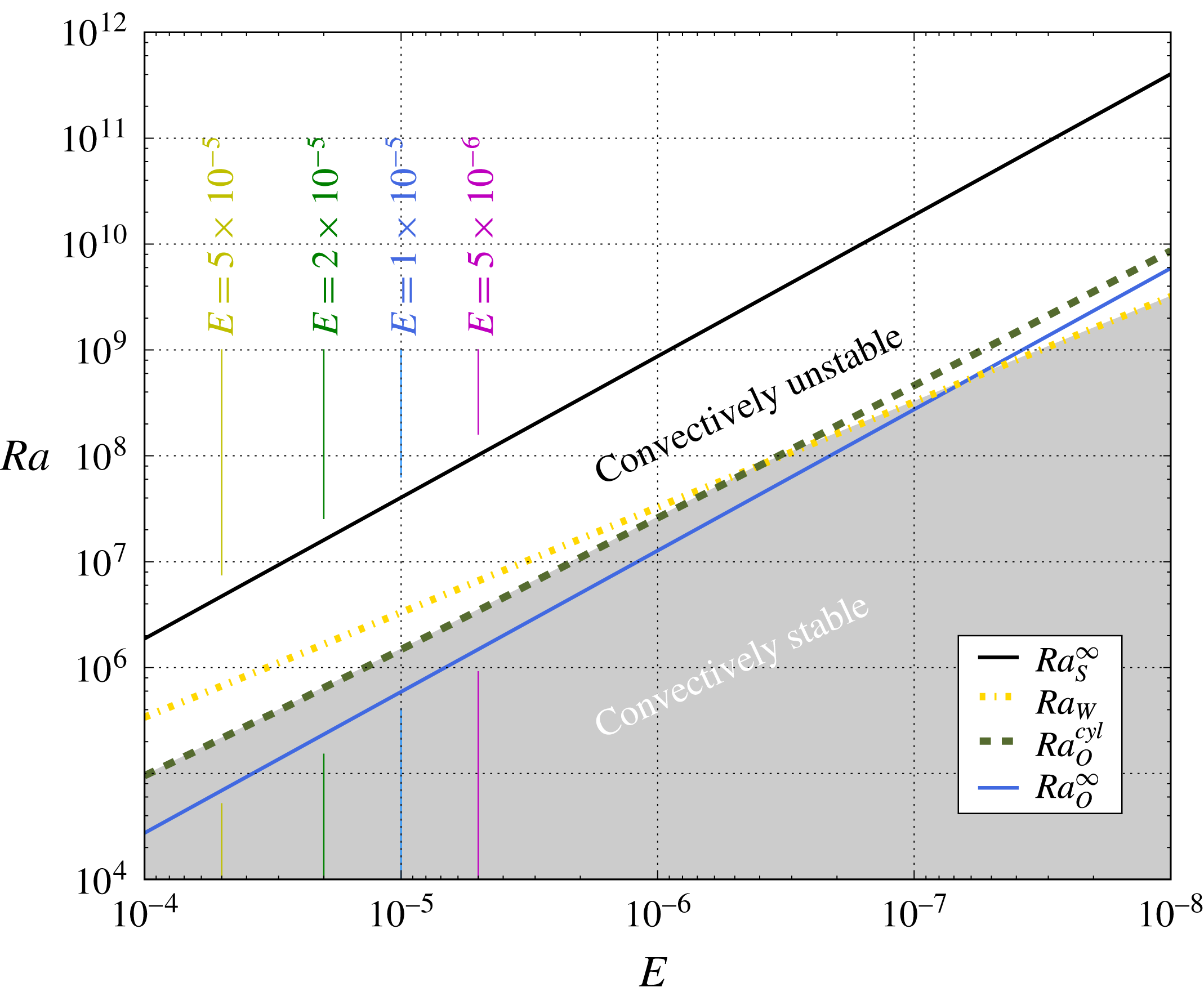
, where buoyancy first overcomes diffusive losses (Chandrasekhar Reference Chandrasekhar1961). However, in contrast to RBC, a number of additional instability mechanisms exist in rotating convection (RC) systems. The theoretical predictions relevant for our cylindrical experimental set-up are discussed below and summarised in figure 1.
Theoretical predictions for the critical Rayleigh numbers
 $Ra$
at convective onset in the limit of rapid rotation plotted as a function of the Ekman number
 $E$
for parameters of our laboratory experiments, aspect ratio
 $\unicode[STIX]{x1D6E4}=1.94$
and Prandtl number
 $Pr=0.025$
. The solid blue and black lines, respectively, denote the infinite plane-layer theoretical estimates for the oscillatory convection
 $Ra_{O}^{\infty }$
and steady convection
 $Ra_{S}^{\infty }$
. The dot-dashed yellow line denotes the onset estimates for the wall modes
 $Ra_{W}$
and the dashed green line marks the asymptotic solution for the onset of oscillatory modes in a cylinder
 $Ra_{O}^{cyl}$
, both taken from Zhang & Liao (Reference Zhang and Liao2009). The grey shaded area marks the convectively stable region; convection occurs in the white area above.

2.2.1 Steady onset
Thermal buoyancy primarily has to overcome the stabilising effects of rotation in RC systems, requiring the critical
 $Ra$
to increase with decreasing
 $E$
(e.g. Chandrasekhar Reference Chandrasekhar1961). Independent of
 $Pr$
, there is a stationary bifurcation connected to the onset of steady rotating convection (
 $S$
) in systems with constant height. This type of convective onset behaviour is also known as the viscous convection mode (Zhang & Liao Reference Zhang and Liao2017). At leading order, friction balances the Coriolis and pressure gradient forces and temporal dependencies do not enter the problem, thus, the velocity derivatives
 $\unicode[STIX]{x2202}_{t}\boldsymbol{u}$
are zero. The linear Navier–Stokes equations then simplify to
 $$\begin{eqnarray}\displaystyle & \displaystyle -2\unicode[STIX]{x1D6FA}\boldsymbol{u}\times \widehat{\boldsymbol{e}}_{z}+{\displaystyle \frac{1}{\unicode[STIX]{x1D70C}}}\unicode[STIX]{x1D735}p-\unicode[STIX]{x1D708}\unicode[STIX]{x1D6FB}^{2}\boldsymbol{u}=0, & \displaystyle\end{eqnarray}$$
where
 $\unicode[STIX]{x1D70C}$
is the density and
 $\widehat{\boldsymbol{e}}_{z}$
the unit vector in the vertical direction.
In the asymptotic limit of small
 $E$
, theoretical analyses in a horizontally infinite plane layer (
 $\infty$
) subject to isothermal boundaries yield a steady onset of convection when the Rayleigh number exceeds the critical value
 $$\begin{eqnarray}\displaystyle & \displaystyle Ra_{S}^{\infty }={\displaystyle \frac{3\unicode[STIX]{x03C0}^{4}}{(2\unicode[STIX]{x03C0}^{4})^{2/3}}}E^{-4/3}=8.7~E^{-4/3}, & \displaystyle\end{eqnarray}$$
occurring in the form of axially elongated structures with non-dimensional horizontal flow scales
 $$\begin{eqnarray}\displaystyle & \displaystyle \ell _{S}^{\infty }={\displaystyle \frac{\unicode[STIX]{x03C0}}{\left({\displaystyle \frac{1}{2}}\unicode[STIX]{x03C0}^{2}\right)^{1/6}}}E^{1/3}=2.4\,E^{1/3} & \displaystyle\end{eqnarray}$$
(e.g. Chandrasekhar Reference Chandrasekhar1961; Julien & Knobloch Reference Julien and Knobloch1998). These theoretical results hold independent of the velocity boundary conditions (e.g. Clune & Knobloch Reference Clune and Knobloch1993).
The stationary steady modes in systems with constant height, such as plane layers or cylinders, correspond to slowly drifting Rossby waves in systems with changing depth, such as spheres and spherical shells (Busse Reference Busse1970). Equation (2.7) still holds, meaning that
 $\unicode[STIX]{x2202}_{t}\boldsymbol{u}$
does not enter the leading-order problem, and that, mathematically, they can be regarded as ‘quasisteady’ modes (Greenspan Reference Greenspan1968). The slow drift is solely due to the varying height in spherical geometries (see Zhang & Schubert Reference Zhang and Schubert2000; Zhang & Liao Reference Zhang and Liao2017, and references therein).
2.2.2 Oscillatory onset
In fluids with
 $Pr<0.68$
, instability in rapidly rotating planar systems sets in at a
 $Ra$
that is lower than
 $Ra_{S}^{\infty }$
, occurring in the form of thermally driven inertial oscillations (e.g. Chandrasekhar Reference Chandrasekhar1961; Julien, Knobloch & Werne Reference Julien, Knobloch, Werne, Banerjee and Eaton1999; Zhang & Liao Reference Zhang and Liao2009). To leading order these inertial convection modes are described by a balance between the inertial, Coriolis and pressure gradient forces:
 $$\begin{eqnarray}\displaystyle & \displaystyle \unicode[STIX]{x2202}_{t}\boldsymbol{u}-2\unicode[STIX]{x1D6FA}\boldsymbol{u}\times \widehat{\boldsymbol{e}}_{z}+{\displaystyle \frac{1}{\unicode[STIX]{x1D70C}}}\unicode[STIX]{x1D735}p=0. & \displaystyle\end{eqnarray}$$
The solution is obtained by making an oscillatory ansatz
 $\boldsymbol{u}\propto \exp (\text{i}\unicode[STIX]{x1D714}t)$
, which then leads to the Poincaré equation (Zhang & Liao Reference Zhang and Liao2017).
In contrast to steady rotating convection, which is solely controlled by
 $E$
, these oscillatory modes are controlled by the value of
 $E/Pr$
, the so-called thermal Ekman number (Julien et al.
Reference Julien, Knobloch, Werne, Banerjee and Eaton1999; Gillet et al.
Reference Gillet, Brito, Jault and Nataf2007). Oscillatory (
 $O$
) convection is predicted to onset in a horizontally infinite plane (
 $\infty$
) at
 $$\begin{eqnarray}\displaystyle & \displaystyle Ra_{O}^{\infty }=6{\displaystyle \frac{\left({\displaystyle \frac{1}{2}}\unicode[STIX]{x03C0}^{2}\right)^{2/3}}{(1+Pr)^{1/3}}}\left({\displaystyle \frac{E}{Pr}}\right)^{-4/3}\simeq 17.4\left({\displaystyle \frac{E}{Pr}}\right)^{-4/3}, & \displaystyle\end{eqnarray}$$
with a larger horizontal length scale than that of steady convection,
 $$\begin{eqnarray}\displaystyle & \displaystyle \ell _{O}^{\infty }=(1+Pr)^{1/3}\frac{\unicode[STIX]{x03C0}}{\left({\displaystyle \frac{1}{2}}\unicode[STIX]{x03C0}^{2}\right)^{1/6}}\,\left({\displaystyle \frac{E}{Pr}}\right)^{1/3}\simeq 2.4\left({\displaystyle \frac{E}{Pr}}\right)^{1/3}. & \displaystyle\end{eqnarray}$$
The normalised oscillation frequency at the onset of these convective motions is estimated to be
 $$\begin{eqnarray}\displaystyle & \displaystyle \widetilde{f}_{O}^{\infty }=4\unicode[STIX]{x03C0}{\displaystyle \frac{(2-3Pr^{2})^{1/2}}{(1+Pr^{2})^{1/3}}}\left({\displaystyle \frac{1}{2}}\unicode[STIX]{x03C0}^{2}\right)^{1/3}\left({\displaystyle \frac{E}{Pr}}\right)^{1/3}\simeq 4.8\left({\displaystyle \frac{E}{Pr}}\right)^{1/3}. & \displaystyle\end{eqnarray}$$
The right-hand expressions in (2.11)–(2.13) all hold for
 $Pr\ll 1$
.
Comparing the linear theoretical predictions for steady and oscillatory low-
 $Pr$
convection yields
 $$\begin{eqnarray}\displaystyle & \displaystyle Ra_{O}^{\infty }/Ra_{S}^{\infty }\simeq 2Pr^{4/3}\quad \text{and}\quad \ell _{O}^{\infty }/\ell _{S}^{\infty }\simeq Pr^{-1/3}. & \displaystyle\end{eqnarray}$$
At a given asymptotically low value of
 $E$
, (2.14a
) implies that
 $Ra_{O}^{\infty }$
will be approximately 70 times smaller than
 $Ra_{S}^{\infty }$
in gallium (
 $Pr\simeq 0.025$
). Further, the asymptotic predictions for the characteristic horizontal length scale of oscillatory motions in (2.14b
) are approximately 3.4 times larger than the corresponding scale for steady rotating convective flows in
 $Pr\simeq 0.025$
fluids. This likely explains the difference in characteristic flow scales found in the low- and high-
 $Pr$
simulations of Calkins et al. (Reference Calkins, Aurnou, Eldredge and Julien2012).
Geometrical confinement has a stabilising effect on oscillatory and stationary rotating convective instabilities, resulting in higher critical
 $Ra$
values for both these instability mechanisms (Goldstein et al.
Reference Goldstein, Knobloch, Mercader and Net1993, Reference Goldstein, Knobloch, Mercader and Net1994). For cylindrical containers, as used in our laboratory experiments, there exist asymptotic predictions in the limit of small
 $E$
and
 $Pr$
by Zhang & Liao (Reference Zhang and Liao2009) that take the finite geometry into account. Minimising their equations (4.21) and (4.22) yields more accurate estimates of the Rayleigh number, oscillation frequency and modal structure than the infinite layer predictions (Horn & Schmid Reference Horn and Schmid2017). The critical Rayleigh number in a cylindrical container is denoted
 $Ra_{O}^{cyl}$
and the oscillation frequency is denoted
 $\widetilde{f}_{O}^{cyl}$
. They approach the values (2.11) and (2.13) for
 $E\rightarrow 0$
, albeit far more slowly than in
 $Pr\gtrsim 1$
fluids (Goldstein et al.
Reference Goldstein, Knobloch, Mercader and Net1994) and at
 $E$
values well below those investigated in our laboratory experiments (figure 1).
In spherical geometries the corresponding solutions to the Poincaré equation yield inertial oscillatory modes that are equatorially trapped and require
 $Pr\lesssim 10^{-3}$
(Zhang Reference Zhang1994, Reference Zhang1995; Zhang & Liao Reference Zhang and Liao2017). For moderately small
 $Pr$
(as considered in the present study), the onset modes in spheres are governed by both viscous and inertial forces, leading to the transitional form of spiralling convection (Zhang & Schubert Reference Zhang and Schubert2000; Kaplan et al.
Reference Kaplan, Schaeffer, Vidal and Cardin2017; Zhang & Liao Reference Zhang and Liao2017).
In shells, convection sets in within the tangent cylinder well after convection outside the tangent cylinder has already commenced, and is already determined by nonlinear dynamics. Thus, linear stability considerations cannot account for the onset behaviour within the tangent cylinder. We hypothesise that inertial convection modes, similar to those existing in plane layers and cylinders, may also manifest at higher latitudes in spherical shells, within the tangent cylinder volume.
2.2.3 Wall modes
Lateral boundaries can help to release the rotational constraint on the fluid, providing an additional source of instability. Through a Hopf bifurcation, wall modes develop in the form of waves that typically precess in the retrograde direction around the periphery of the tank (e.g. Zhong, Ecke & Steinberg Reference Zhong, Ecke and Steinberg1991; Herrmann & Busse Reference Herrmann and Busse1993; Goldstein et al.
Reference Goldstein, Knobloch, Mercader and Net1994; Bajaj, Ahlers & Pesch Reference Bajaj, Ahlers and Pesch2002). Assuming that the curvature of the cylinder can be neglected, and for a no-slip, thermally insulated sidewall and no-slip, isothermal top and bottom boundaries, wall modes are predicted at low
 $E$
to first develop at (Herrmann & Busse Reference Herrmann and Busse1993; Liao, Zhang & Chang Reference Liao, Zhang and Chang2006; Zhang & Liao Reference Zhang and Liao2009)
 $$\begin{eqnarray}\displaystyle & \displaystyle Ra_{W}=\unicode[STIX]{x03C0}^{2}(6\sqrt{3})^{1/2}E^{-1}+46.55E^{-2/3}\simeq 31.8E^{-1}+46.6E^{-2/3}, & \displaystyle\end{eqnarray}$$
 $$\begin{eqnarray}\displaystyle & \displaystyle m_{W}={\displaystyle \frac{2\unicode[STIX]{x03C0}}{2\ell _{W}}}\simeq \unicode[STIX]{x1D6E4}(3.03-17.5E^{1/3}), & \displaystyle\end{eqnarray}$$
where we take
 $2\ell _{W}$
as the wall mode wavelength and note that (2.16) applies at the tank’s periphery where the wall modes are localised. Their drift frequency is given by
 $$\begin{eqnarray}\displaystyle & \displaystyle \widetilde{f}_{W}=4\unicode[STIX]{x03C0}^{2}\sqrt{3}(2+\sqrt{3})^{1/2}{\displaystyle \frac{E}{Pr}}-1464.53{\displaystyle \frac{E^{4/3}}{Pr}}\simeq 131.8{\displaystyle \frac{E}{Pr}}-1464.5{\displaystyle \frac{E^{4/3}}{Pr}}. & \displaystyle\end{eqnarray}$$
Wall modes are a special type of the viscous convection mode (Zhang & Liao Reference Zhang and Liao2017) and do not have an exact equivalent in spherical geometries as they form on thermally passive lateral walls. However, slowly oscillatory, wall-mode-like flows have been argued to form at the virtual boundary of the tangent cylinder in the laboratory experiments of Aujogue et al. (Reference Aujogue, Pothérat, Sreenivasan and Debray2018).
2.2.4 Onset predictions for the laboratory set-up
The critical Rayleigh number predictions
 $Ra_{S}^{\infty }$
,
 $Ra_{O}^{\infty }$
,
 $Ra_{O}^{cyl}$
and
 $Ra_{W}$
are plotted in figure 1 as a function of the Ekman number and employing our experimentally fixed values of
 $\unicode[STIX]{x1D6E4}=1.94$
and
 $Pr\simeq 0.025$
. Based on these onset curves and the four
 $E$
values employed in our experiments, we argue that
 $Ra_{O}^{cyl}$
is the most appropriate choice to evaluate the supercriticality of the cases investigated. In the following, we will denote the supercriticality as
 $\widetilde{Ra}=Ra/Ra_{O}^{cyl}$
.
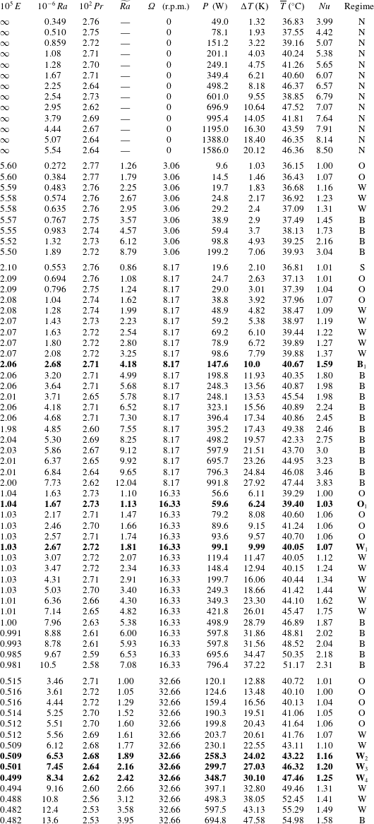
Table 1 contains the theoretical onset parameter predictions for the four Ekman numbers of our survey, including the critical Rayleigh numbers, the onset frequencies and the ratios of the critical Rayleigh numbers relative to
 $Ra_{O}^{cyl}$
.
The values of
 $\widetilde{Ra}_{S}^{\infty }$
range from 20 to 30 for our experimental cases. In all the experiments, however,
 $\widetilde{Ra}\lesssim 12$
(table 3), which implies that none of the behaviours found in our experiments are the result of steady rotating convective flow processes. Thus, the quasisteady columnar convection modes that dominate models of
 $Pr\gtrsim 1$
rotating convection (e.g. Grooms et al.
Reference Grooms, Julien, Weiss and Knobloch2010; King & Aurnou Reference King and Aurnou2012; Gastine, Wicht & Aubert Reference Gastine, Wicht and Aubert2016) and dynamo action (e.g. Christensen Reference Christensen2011; Jones Reference Jones2011; Schaeffer et al.
Reference Schaeffer, Jault, Nataf and Fournier2017) are non-existent in the experimental simulations carried out here.
Furthermore, due to gallium’s low-
 $Pr$
value, oscillatory convective motions develop before wall modes for
 $E\gtrsim 5\times 10^{-7}$
. Thus, the regime in which wall modes are the onset mode cannot be investigated here since all our experiments are performed at
 $E>10^{-6}$
. This is a clear distinction from moderate-
 $Pr$
fluids, where wall modes are always the preferred onset behaviour in finite containers (Zhong, Ecke & Steinberg Reference Zhong, Ecke and Steinberg1993).
We also note that Zhang & Liao (Reference Zhang and Liao2009) provide some linear stability calculations of the onset values. For the case at
 $E=5\times 10^{-5}$
,
 $Pr=0.025$
and
 $\unicode[STIX]{x1D6E4}=4$
, they find a critical Rayleigh number for oscillatory convection that is about 5 % higher than their asymptotic
 $Ra_{O}^{cyl}$
predictions. These differences provide a minor source of uncertainty for our onset predictions. The deviations in the onset frequency are, on the other hand, insignificant.
Asymptotic estimates of the onset parameters of liquid gallium with
 $Pr=0.025$
and for the experimentally employed Ekman numbers
 $E$
. They are discussed in detail in § 2.2. The critical Rayleigh numbers
 $Ra_{O}^{cyl}$
and the corresponding frequencies
 $\widetilde{f}_{O}^{cyl}$
are calculated for
 $\unicode[STIX]{x1D6E4}=1.94$
. All frequencies are normalised by
 $f_{\unicode[STIX]{x1D6FA}}$
: see (2.4). In addition, the ratios of the critical Rayleigh numbers and
 $Ra_{O}^{cyl}$
are shown with tildes:
 $\widetilde{Ra}_{O}^{\infty }\equiv Ra_{O}^{\infty }/Ra_{O}^{cyl}$
,
 $\widetilde{Ra}_{W}\equiv Ra_{W}/Ra_{O}^{cyl}$
and
 $\widetilde{Ra}_{S}^{\infty }\equiv Ra_{s}^{\infty }/Ra_{O}^{cyl}$
.

3 Experimental set-up
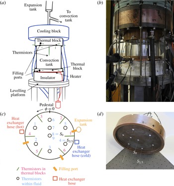
(a) Schematic of the experimental set-up, adapted from King, Stellmach & Aurnou (Reference King, Stellmach and Aurnou2012). (b) Image of the experimental set-up, while the tank is being filled with gallium. For scale, the acrylic sidewall outer diameter is 20.0 cm. (c) Top view schematic of the positions of the thermistors in and below the top thermal block. (d) Oblique view of the top thermal block showing internal thermistors located at the ends of the thin stainless steel rods. The eighth and fourth sensors, whose data are discussed in detail throughout the paper, are respectively marked
 $S_{0}$
and
 $S_{2/3}$
. The respective positions of
 $S_{0}$
and
 $S_{2/3}$
are
 $(r/R_{i}=0.01,\,\unicode[STIX]{x1D719}=0^{\circ },\,z/H=0.487)$
and
 $(r/R_{i}=0.70,\,\unicode[STIX]{x1D719}=240^{\circ },\,z/H=0.431)$
, with
 $R_{i}=9.7~\text{cm}$
and
 $H=10.0~\text{cm}$
being the inner radius and height of the fluid layer and the axial
 $z$
-coordinate value increasing positively upwards from the base of the fluid layer where
 $z/H=0$
.

The laboratory set-up consists of a Rayleigh–Bénard convection (RBC) device that is seated on a rotating pedestal, as shown in figure 2. All the experiments are carried out in an axially aligned cylindrical container with height
 $H=10.0~\text{cm}$
and inner radius
 $R_{i}=9.7~\text{cm}$
. Consequently, the diameter is
 $D=19.4~\text{cm}$
and the aspect ratio is fixed at
 $\unicode[STIX]{x1D6E4}=1.94$
. The cylindrical sidewall is made of Reynolds R-Cast acrylic, which has a thermal conductivity of
 $k=0.2~\text{W}~(\text{m}\,\text{K})^{-1}$
, which is less than 1 % that of gallium. The fluid is heated from below by a non-inductively wound, electrical resistance element, which is placed below a bottom copper thermal block of 1.5 cm thickness. The input power varies from
 $P=10~\text{W}$
to 2 kW. After accounting for thermal losses,
 $P_{loss}$
, the input power is used to estimate
 $Q_{tot}=(P-P_{loss})/A$
, the total vertical heat flow across the fluid layer of horizontal cross-sectional area
 $A=\unicode[STIX]{x03C0}R_{i}^{2}$
. Heat is removed from the system by a double-spiral wound heat exchanger maintained at a constant temperature by a Thermo-NESLab HX-300 precision thermal bath. This heat exchanger is placed above a top copper thermal block of 4 cm thickness.
The vertical temperature difference across the fluid layer,
 $\unicode[STIX]{x0394}T$
, is measured using two arrays of six thermistors each embedded in the top and bottom thermal blocks, 2 mm above and below the fluid layer, respectively. In addition, nine ‘internal’ thermistors are located inside the fluid layer. The locations of the thermistors are shown in figure 2(c,d). The temperature drop from the bottom to the top of the tank varies from 1 K to 50 K and the mean fluid temperature varies from
 $36~^{\circ }\text{C}$
to
 $55~^{\circ }\text{C}$
. Isothermal boundary conditions are adequately maintained, with a maximum Biot number of
 $Bi=Nu(k_{fluid}/k_{boundary})(H_{boundary}/H_{fluid})=0.27$
in the top thermal block of our highest-
 $Ra$
RBC case. Temperatures and heating rate are recorded via a National Instruments data acquisition system that is located in the rotating frame and acquires data at 10 samples per second. The system is assumed to have equilibrated when the mean temperature,
 $\overline{T}$
, on each thermistor does not change by more than
 $1$
% during the previous 30 min. We then record equilibrated data for up to 10 h (
 ${\sim}45\unicode[STIX]{x1D70F}_{\unicode[STIX]{x1D705}}$
). The tank is insulated on all sides by two layers of thermal insulating materials. The outer layer is an
 ${\sim}5~\text{cm}$
thick Insulfrax fibrous insulation and the inner layer is an
 ${\sim}10~\text{cm}$
thick layer of closed cell foam. K-type thermocouples placed within the two insulation layers enable us to estimate the sidewall heat losses. The motion of the rotating pedestal is controlled by a belt-driven brushless servomotor. The rotation rate can be varied between 0 to 60 revolutions per minute (r.p.m.). In this study, four rotation rates are investigated: 3.06 r.p.m., 8.17 r.p.m., 16.33 r.p.m. and 32.66 r.p.m. See the supplementary material in King et al. (Reference King, Stellmach and Aurnou2012) for further device details.
3.1 Material properties of gallium
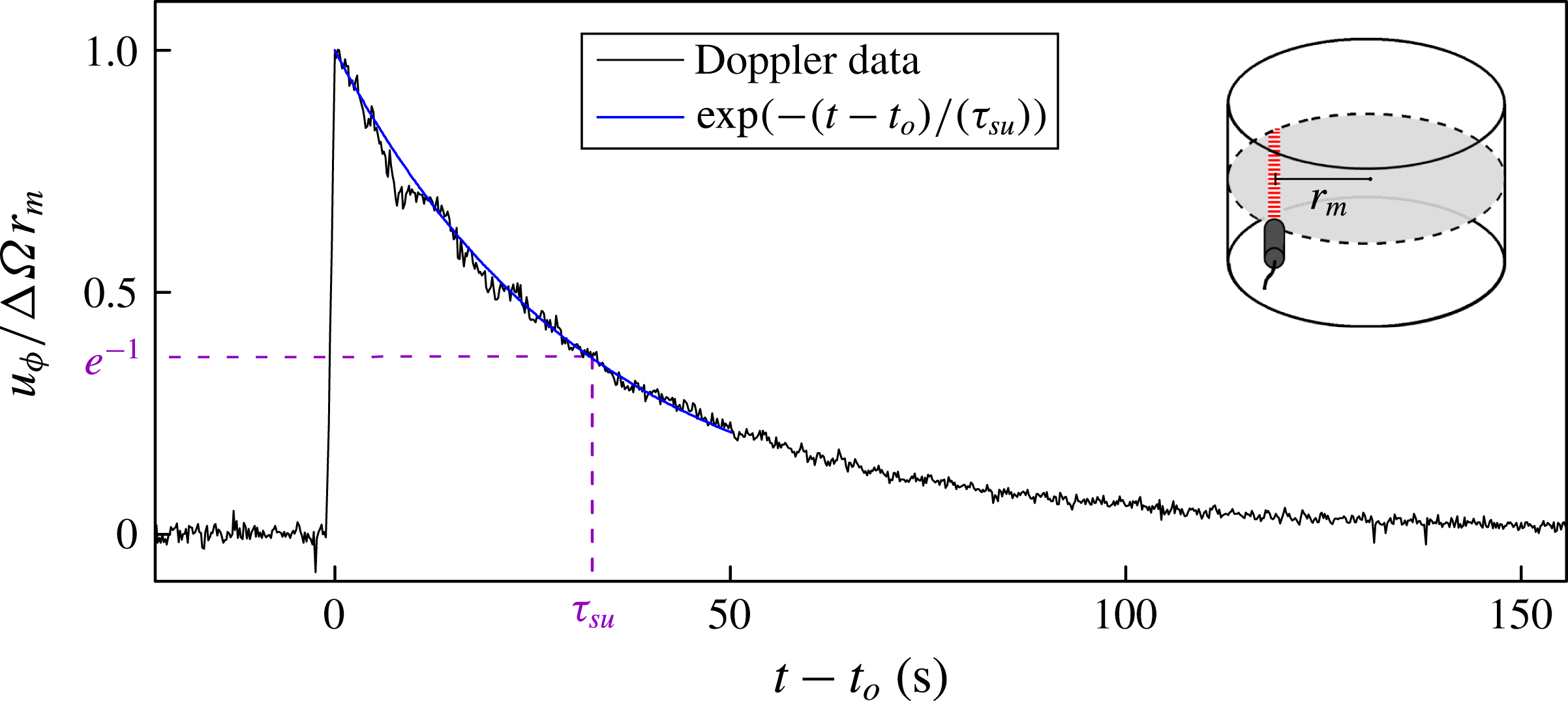
Acoustic Doppler velocimetry measurement (black line) of a spin-up experiment carried out at
 $T=35.8~^{\circ }\text{C}$
. The data show the temporal evolution of the midplane azimuthal velocity,
 $u_{\unicode[STIX]{x1D719}}$
, normalised by the maximum predicted spin-up velocity,
 $(\unicode[STIX]{x0394}\unicode[STIX]{x1D6FA}\,r_{m})$
. Here
 $\unicode[STIX]{x0394}\unicode[STIX]{x1D6FA}$
is the impulsive change in rotation rate occurring at time
 $t_{o}$
, and
 $r_{m}$
is the radial position at the midpoint along the Doppler chord (inset). We denote the spin-up time,
 $\unicode[STIX]{x1D70F}_{su}$
, as the point in the time series where the normalised velocity reaches a value of
 $1/\text{e}$
(dashed purple lines). The blue line shows the exponential decay with the characteristic time scale
 $\unicode[STIX]{x1D70F}_{su}$
.

Liquid gallium’s material properties are not well-determined. Most notable is its viscosity, where the available measurements are not only scarce but exhibit deviations of almost 40 % (Spells Reference Spells1936; Predel & Arpshofen Reference Predel and Arpshofen1968; Genrikh, Kaplun & Solovev Reference Genrikh, Kaplun and Solovev1972; Iida, Morita & Takeuchi Reference Iida, Morita and Takeuchi1975). Reasons for this difficulty are, amongst others, that gallium is a semi-metal, and also its affinity to oxygen, leading to the formation of gallium oxides that contaminate the bulk fluid.
This translates into inaccuracies in the derived dimensionless parameters, such as
 $Ra$
,
 $Pr$
,
 $E$
and
 $Nu$
. Hence, values of gallium’s material properties are the main source of uncertainty with regard to the comparison of our laboratory results and theoretical predictions. Moreover, knowledge of the non-dimensional control parameters is also essential in order to be able to carry out comparative numerical studies (see Stellmach et al.
Reference Stellmach, Lischper, Julien, Vasil, Cheng, Ribeiro, King and Aurnou2014). Thus, while unavoidable, we have strived to minimise the uncertainty in the material properties as much as possible.
To obtain accurate viscosity values, we have carried out a separate suite of experiments in which we use acoustic Doppler velocimetry (Vogt et al.
Reference Vogt, Grants, Räbiger, Eckert and Gerbeth2012, Reference Vogt, Grants, Eckert and Gerbeth2013; Vogt, Räbiger & Eckert Reference Vogt, Räbiger and Eckert2014) to measure linear spin-up in our tank of gallium under nearly isothermal conditions (see Brito, Aurnou & Cardin Reference Brito, Aurnou and Cardin2004). In these experiments, the tank is spun up in less than 1 s (fixed
 $4~\text{r.p.m.}~\text{s}^{-1}$
ramp) from an initial rotation rate
 $\unicode[STIX]{x1D6FA}_{i}$
to a final rotation rate
 $\unicode[STIX]{x1D6FA}_{i}+\unicode[STIX]{x0394}\unicode[STIX]{x1D6FA}$
. The azimuthal velocity,
 $u_{\unicode[STIX]{x1D719}}$
, is measured along a midplane chord at a radial position
 $r_{m}\simeq 0.70R_{i}$
(inset, figure 3).
Figure 3 shows normalised Doppler velocity measurements,
 $u_{\unicode[STIX]{x1D719}}/\unicode[STIX]{x0394}\unicode[STIX]{x1D6FA}\,r_{m}$
, versus time
 $t$
shifted relative to
 $t_{o}$
, the instant of peak measured velocity. The fluid temperature is
 $T=35.8~^{\circ }\text{C}$
here and the spin-up goes from 40.0 r.p.m. to 44.0 r.p.m. (
 $\unicode[STIX]{x0394}\unicode[STIX]{x1D6FA}/\unicode[STIX]{x1D6FA}_{i}=0.1$
). The fluid responds via an exponential temporal adjustment to the new solid-body rotation rate. This occurs on the spin-up time scale
 $$\begin{eqnarray}\displaystyle & \displaystyle \unicode[STIX]{x1D70F}_{su}=(8E)^{-1/2}\,\unicode[STIX]{x1D6FA}_{i}^{-1}=H/(2\sqrt{\unicode[STIX]{x1D708}\unicode[STIX]{x1D6FA}_{i}}) & \displaystyle\end{eqnarray}$$
(Greenspan & Howard Reference Greenspan and Howard1963; Greenspan Reference Greenspan1969; Warn-Varnas et al.
Reference Warn-Varnas, Fowlis, Piacsek and Lee1978). We estimate
 $\unicode[STIX]{x1D70F}_{su}$
here as the time at which the
 $u_{\unicode[STIX]{x1D719}}/\unicode[STIX]{x0394}\unicode[STIX]{x1D6FA}\,r_{m}=\exp (-1)$
. From
 $\unicode[STIX]{x1D70F}_{su}$
, the kinematic viscosity at a fixed temperature is inferred.
The formulation of Andrade (Reference Andrade1934) is used to best fit our gallium viscosity data as a function of (absolute) temperature,
 $$\begin{eqnarray}\displaystyle & \displaystyle \unicode[STIX]{x1D702}=\unicode[STIX]{x1D702}_{0}\,\exp \left({\displaystyle \frac{E_{a}}{R\,T}}\right), & \displaystyle\end{eqnarray}$$
where the activation energy is
 $E_{a}=4000~\text{J}~\text{mol}^{-1}$
, the gas constant is
 $R=8.3144~\text{J}~(\text{mol}~\text{K})^{-1}$
and the dynamic viscosity coefficient is determined from our spin-up data to be
 $\unicode[STIX]{x1D702}_{0}=0.46~\text{mPa}~\text{s}$
, in adequate agreement with the values of Spells (Reference Spells1936), Iida et al. (Reference Iida, Morita and Takeuchi1975), Brandes & Brook (Reference Brandes and Brook1992) and King & Aurnou (Reference King and Aurnou2013). See appendix § A.1 for further details.
We have also measured the in situ value of liquid gallium’s thermal conductivity in experiments in which the fluid layer was convectively stable (see figure 10 and table 2). In conjunction with Fourier’s law of conduction, we obtain a thermal conductivity value of
 $$\begin{eqnarray}\displaystyle k=(31.4\pm 0.1)\text{W}~(\text{m}~\text{K})^{-1}, & & \displaystyle\end{eqnarray}$$
which agrees well with other, independent, laboratory estimations (Aurnou & Olson Reference Aurnou and Olson2001; King & Aurnou Reference King and Aurnou2013). See appendix § A.2 for details of this method.
Liquid gallium’s density is well constrained and is taken to vary with temperature as
 $$\begin{eqnarray}\displaystyle & \displaystyle \unicode[STIX]{x1D70C}(T)=\unicode[STIX]{x1D70C}_{mp}(1-\unicode[STIX]{x1D6FC}(T-T_{mp})), & \displaystyle\end{eqnarray}$$
where
 $\unicode[STIX]{x1D70C}_{mp}=6.09\times 10^{3}~\text{kg}~\text{m}^{-3}$
is the density at the melting point,
 $\unicode[STIX]{x1D6FC}=1.25\times 10^{-4}~\text{K}^{-1}$
is the thermal expansion coefficient and
 $T_{mp}=29.8~^{\circ }\text{C}$
is the melting point (Spells Reference Spells1936; Brandes & Brook Reference Brandes and Brook1992; Assael et al.
Reference Assael, Armyra, Brillo, Stankus, Wu and Wakeham2012). Similarly, gallium’s specific heat capacity is only weakly temperature dependent and these variations are usually smaller than the accuracy of the measurement over the temperature range of our experiments. Thus, we chose a constant value of
 $$\begin{eqnarray}\displaystyle C_{p}=397.6~\text{J}~(\text{kg}~\text{K})^{-1}, & & \displaystyle\end{eqnarray}$$
as reported in Brandes & Brook (Reference Brandes and Brook1992) and used in prior studies with this device (e.g. King & Aurnou Reference King and Aurnou2015).
4 Results
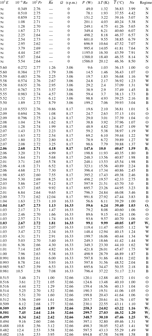
We have carried out a suite of laboratory convection experiments consisting of 13 non-rotating and 61 rotating cases, summarised in table 3 in the appendix. Our experiments produce a comprehensive picture of oscillatory and wall-localised convection in low-
 $Pr$
fluids. In the following, we will mainly focus on six selected cases that reflect the characteristic behaviour of each regime. These are:
 $\text{O}_{1}$
:
 $E=1.04\times 10^{-5},\;Ra=1.67\times 10^{6},\,\widetilde{Ra}=1.13$
in the purely oscillatory regime;
 $\text{W}_{1}$
:
 $E=1.03\times 10^{-5},\;Ra=2.67\times 10^{6},\,\widetilde{Ra}=1.83$
in the wall mode regime;
 $\text{W}_{2}$
:
 $E=5.09\times 10^{-6},\;Ra=6.53\times 10^{6},\,\widetilde{Ra}=1.89$
in the wall mode regime;
 $\text{W}_{3}$
:
 $E=5.01\times 10^{-6},\;Ra=7.45\times 10^{6},\,\widetilde{Ra}=2.16$
in the wall mode regime;
 $\text{W}_{4}$
:
 $E=4.99\times 10^{-6},\;Ra=8.34\times 10^{6},\,\widetilde{Ra}=2.42$
in the wall mode regime; and
 $\text{B}_{1}$
:
 $E=2.06\times 10^{-5},\;Ra=2.68\times 10^{6},\,\widetilde{Ra}=4.18$
in the broad-band regime.
4.1 Spectral analysis
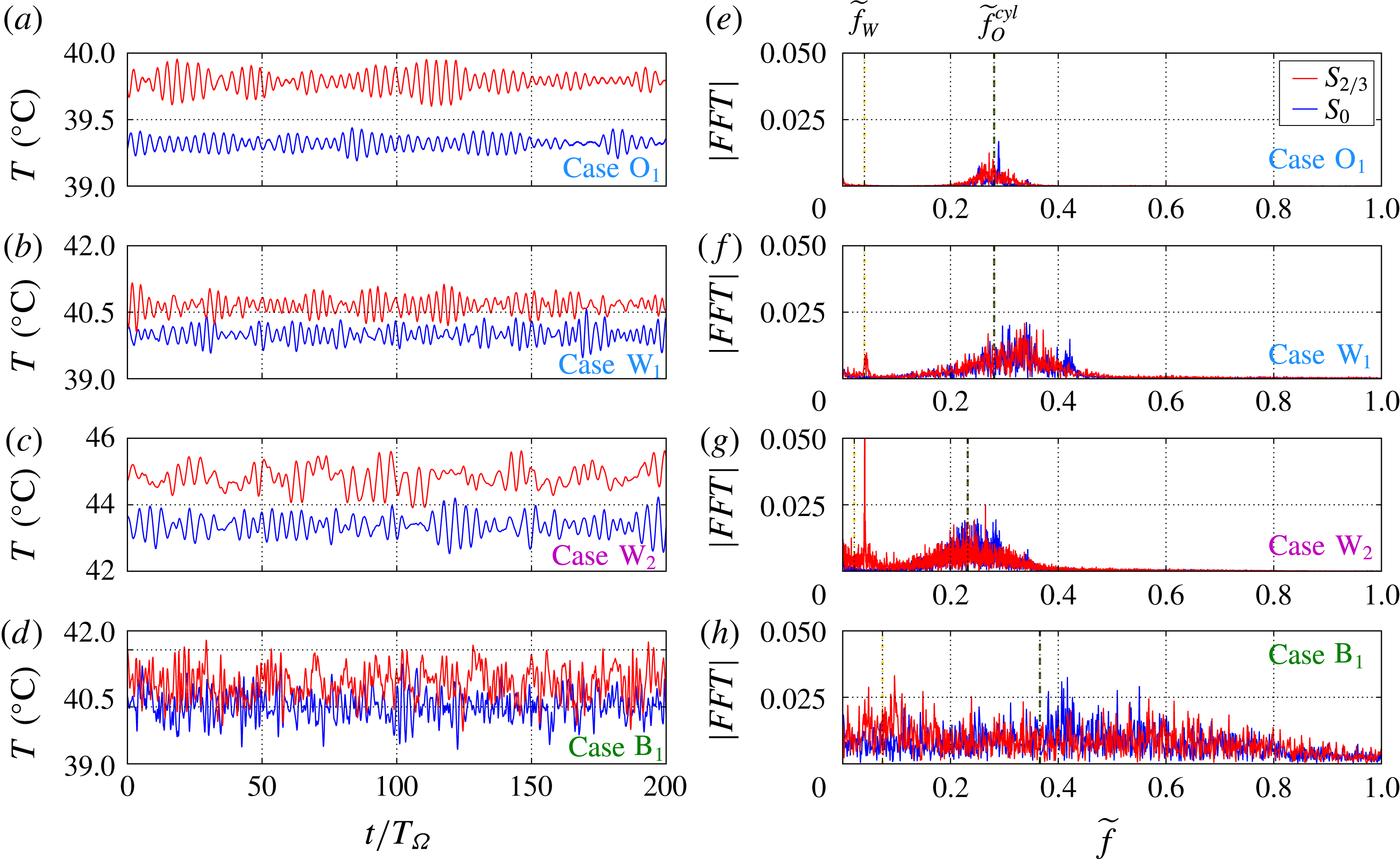
(a–d) Temperature time series recorded on thermistors
 $S_{2/3}$
(red) and
 $S_{0}$
(blue) in cases
 $\text{O}_{1}$
,
 $\text{W}_{1}$
, W
 $_{2}$
,
 $\text{B}_{1}$
for 200 rotation periods
 $T_{\unicode[STIX]{x1D6FA}}$
of the tank. (e–h) The Fourier transform of the temperature signals computed over 290
 $T_{\unicode[STIX]{x1D6FA}}$
for case
 $\text{O}_{1}$
, over 1152
 $T_{\unicode[STIX]{x1D6FA}}$
for case
 $\text{W}_{1}$
, over 3580
 $T_{\unicode[STIX]{x1D6FA}}$
for case W
 $_{2}$
, and over 853
 $T_{\unicode[STIX]{x1D6FA}}$
for case
 $\text{B}_{1}$
. The dashed green (dot-dashed yellow) lines correspond to the onset frequencies of bulk oscillatory modes (wall modes). Note that the thermal diffusion frequencies,
 $\widetilde{f}_{\unicode[STIX]{x1D705}}=2E/Pr$
, are
 $7.6\times 10^{-4}$
for
 $\text{O}_{1}$
and
 $\text{W}_{1}$
,
 $3.8\times 10^{-4}$
for W
 $_{2}$
, and
 $1.5\times 10^{-3}$
for
 $\text{B}_{1}$
.

We first present an analysis of the temperature time series and the corresponding spectra obtained with our interior thermistors. While our results are corroborated by all sensors, we concentrate for the sake of clarity on only two of them:
 $S_{0}$
, which is located at the centre of the cylinder, and
 $S_{2/3}$
, which is located closer to the sidewall, near to two-thirds radius. Both sensors are set slightly below the midplane. Their exact positions are
 $(r/R_{i}=0.01,\,\unicode[STIX]{x1D719}=0^{\circ },\,z/H=0.487)$
and
 $(r/R_{i}=0.70,\,\unicode[STIX]{x1D719}=240^{\circ },\,z/H=0.431)$
, respectively, as shown in figures 2(c,d).
Figures 4(a–d) show temperature time series measurements recorded by
 $S_{0}$
and
 $S_{2/3}$
from cases
 $\text{O}_{1}$
,
 $\text{W}_{1}$
, W
 $_{2}$
and
 $\text{B}_{1}$
, each plotted for 200 rotation periods
 $T_{\unicode[STIX]{x1D6FA}}$
. Figures 4(e–h) show the respective temperature spectra from their equilibrated time series (typically
 ${\gtrsim}$
2 h in length). The time series in figure 4(a–d) show coherent oscillations for case
 $\text{O}_{1}$
and increasingly broad-band signals in each of the successive cases
 $\text{W}_{1}$
, W
 $_{2}$
and
 $\text{B}_{1}$
. The spectra shown in images in (e–h) are more revealing of the physics at play. In case
 $\text{O}_{1}$
, carried out at
 $\widetilde{Ra}=1.13$
, oscillations exist in a finite band around the predicted value
 $\widetilde{f}_{O}^{cyl}$
on both thermistors. In case
 $\text{W}_{1}$
, carried out at
 $\widetilde{Ra}=1.83$
, the width of the frequency band around
 $\widetilde{f}_{O}^{cyl}$
has expanded. Furthermore, there is also evidence for a wall mode on thermistor
 $S_{2/3}$
. In case W
 $_{2}$
, carried out at
 $\widetilde{Ra}=1.89$
, the wall mode signal on
 $S_{2/3}$
is now the dominant spectral peak. In addition, the wall mode frequency has shifted to
 $\widetilde{f}=0.0406$
, which is nearly twice the predicted wall mode frequency
 $\widetilde{f}_{W}=0.023$
at onset, suggesting a possible change in wall mode structure. This approximate doubling in wall mode frequency has also been in observed in direct numerical simulations (DNS) at comparable control parameters (Horn & Schmid Reference Horn and Schmid2017). Lastly, in case
 $\text{B}_{1}$
at
 $\widetilde{Ra}=4.18$
, the coherent oscillatory signals are no longer readily apparent. However, the spectrum of the side thermistor
 $S_{2/3}$
has more power near the theoretical wall mode frequency than the central thermistor
 $S_{0}$
, which has slightly more power closer to the bulk oscillation frequency. This suggests that the original instability mechanisms still influence the flow, but are harder to decipher in the broad-band spectra generated on both sensors at these higher
 $\widetilde{Ra}$
values. Accordingly, wall modes and bulk oscillatory modes coexist within our experiment, and our laboratory data provide the first experimental evidence of this multi-modal flow in low-
 $Pr$
rotating convection.
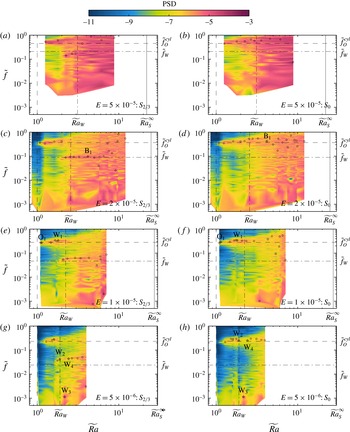
Maps of the power spectral density PSD of the non-dimensional temperature signal
 $(T-\overline{T})/\unicode[STIX]{x0394}\,T$
as a function of
 $\widetilde{f}$
and
 $\widetilde{Ra}$
for (a,b)
 $E=5\times 10^{-5}$
, (c,d)
 $E=2\times 10^{-5}$
, (e,f)
 $E=1\times 10^{-5}$
, and (g,h)
 $E=5\times 10^{-6}$
. (a,c,e,g) Data obtained by the near-wall sensor
 $S_{2/3}$
; (b,d,f,h) data obtained by the central sensor
 $S_{0}$
. The vertical dashed line denotes
 $\widetilde{Ra}_{O}^{cyl}$
, the vertical dot-dashed line
 $\widetilde{Ra}_{W}$
, and the vertical solid line
 $\widetilde{Ra}_{S}^{\infty }$
. The horizontal dashed line marks
 $\widetilde{f}_{O}^{cyl}$
and the horizontal dot-dashed line
 $\widetilde{f}_{W}$
. The dominant spectral frequencies are denoted by circles and stars, respectively, with the stars corresponding to the cases
 $\text{O}_{1}$
,
 $\text{W}_{1}$
–
 $\text{W}_{4}$
and
 $\text{B}_{1}$
. The exact parameters for all cases are given in table 3. Note that the first case for
 $E=2\times 10^{-5}$
is subcritical, while the first case of
 $E=5\times 10^{-6}$
is supercritical and shows a distinct peak at
 $\widetilde{f}_{O}^{cyl}$
; however, the maximum PSD is not contained in that frequency; both cases are marked by grey circles.

To further demonstrate the inherent multi-modality of low-
 $Pr$
RC, we present maps of the power spectral density (PSD) of the non-dimensional temperature
 $(T-\overline{T})/\unicode[STIX]{x0394}\,T$
, plotted as function
 $\widetilde{Ra}$
for the entire experimentally investigated RC parameter space in figure 5. The juxtaposition of the spectrograms obtained by the near-wall thermistor
 $S_{2/3}$
(figure 5
a,c,e,g) and the central thermistor
 $S_{0}$
(figure 5
b,d,f,h) provides a complete picture of the evolution of the dominant processes occurring with increasing supercriticality
 $\widetilde{Ra}$
, and also decreasing
 $E$
. In addition, we mark the position of the maximum spectral power for each case, using star symbols for
 $\text{O}_{1}$
,
 $\text{B}_{1}$
,
 $\text{W}_{1}$
–
 $\text{W}_{4}$
and open circles for all other cases.
The maximum PSD occurs at frequencies close to
 $\widetilde{f}_{O}^{cyl}$
on both thermistors
 $S_{2/3}$
and
 $S_{0}$
in all cases with
 $\widetilde{Ra}\lesssim 0.8\widetilde{Ra}_{W}$
. This indicates that bulk oscillatory convection is dominant over this range. It is also evident that the frequency band containing the maximum PSD broadens out as
 $Ra$
increases beyond oscillatory onset, i.e.,
 $\widetilde{Ra}\gtrsim 1$
. This implies that there are a multitude of oscillatory modes that have critical Rayleigh numbers close to each other, in agreement with theory (Goldstein et al.
Reference Goldstein, Knobloch, Mercader and Net1994).
In the central region of the tank, sampled by
 $S_{0}$
, the maximum PSD resides in the frequency band around
 $\widetilde{f}_{O}^{cyl}$
up to
 $\widetilde{Ra}\lesssim 6$
. In contrast, closer to the sidewall, sampled by
 $S_{2/3}$
, the maximum PSD is contained in frequencies around
 $\widetilde{f}_{W}$
for
 $\widetilde{Ra}\gtrsim 0.8\widetilde{Ra}_{W}$
while the PSD in the
 $\widetilde{f}_{O}^{cyl}$
band becomes depleted. This effect is more discernible for smaller
 $E$
. In this parameter range, then, the wall modes are likely governing the flow dynamics. We note further that the prominent frequency ridge of the wall modes shows an initial increase of
 $\widetilde{f}$
with
 $\widetilde{Ra}$
, as is characteristic for instabilities stemming from a Hopf bifurcation.
The change from bulk oscillatory to wall-mode-dominated convection does not happen abruptly. Because of this relatively smooth transition, the maximum PSD value does not specify the onset value of wall mode convection. For example, the
 $S_{2/3}$
spectrum of case
 $\text{W}_{1}$
shown in figure 4(f) has significant power at
 $\widetilde{f}_{W}$
, but the peak amplitude in the spectrum still resides just above
 $\widetilde{f}_{O}^{cyl}$
.
In addition to power near
 $\widetilde{f}_{O}^{cyl}$
and
 $\widetilde{f}_{W}$
, a peak at very low frequency develops on both the
 $S_{2/3}$
and
 $S_{0}$
sensors in several cases. This is most visible in case
 $\text{W}_{3}$
in figure 5(g). This low-frequency behaviour will be considered further in § 4.3.
In our laboratory experiments, the wall modes onset at
 $Ra$
values that are approximately 20 % below the theoretical predictions (2.15). Possible reasons for these differences are, for example, that low-
 $Pr$
fluids often show a slower convergence to asymptotic solutions. This appears plausible, considering that (2.15) is derived in the limit of
 $E\rightarrow 0$
and zero curvature of the cylinder, and that the agreement between the theoretical
 $\widetilde{Ra}_{W}$
and the actual onset of wall modes becomes better with decreasing
 $E$
. It could be possible that the deviations are caused by imperfect sidewall thermal boundary conditions. Alternatively, the active bulk oscillatory convective motions might affect the system near the sidewalls, such that the wall mode onset properties are altered (Geoff Vasil, private communication). This would mean that the bulk oscillatory modes help to trip the wall modes at values below
 $\widetilde{Ra}_{W}$
. In contrast, the observed deviations in wall mode onset are unlikely to be caused by centrifugal buoyancy effects (Curbelo et al.
Reference Curbelo, Lopez, Mancho and Marques2014), since the Froude number
 $Fr=\unicode[STIX]{x1D6FA}^{2}R_{i}/g$
, which attains a maximum value of 0.12 in our experiments, increases with decreasing
 $E$
, whereas the discrepancy between the experimental results and the theoretical
 $Ra_{W}$
predictions becomes smaller. Finally, our lack of knowledge of the exact material properties, as discussed in § 3.1, might contribute to the discrepancy. However, even if we assume that the error in the viscosity was as high as 40 %, the relevant parameter values are shifted, but the discrepancy between theoretical
 $Ra_{W}$
predictions and our measurements still persists. Thus, our choice of thermophysical properties cannot explain this result. (We refer the reader to Okada & Ozoe (Reference Okada and Ozoe1992) for a complete error analysis in magnetoconvection experiments using liquid gallium.)
Figure 5 reveals broad-band signals for relatively low supercriticalities of
 $\widetilde{Ra}\gtrsim 4$
, far below the expected bifurcation to steady convection (
 $\widetilde{Ra}_{S}^{\infty }\gtrsim 20$
; table 1). We interpret these broad-band signals as signatures of rotating convective turbulence that develops from the nonlinear interaction of inertial modes, and, subsequently, leads to their break-up. Thus, turbulent convection develops in gallium well before steady columnar-style convection even onsets, in basic agreement with Julien et al. (Reference Julien, Rubio, Grooms and Knobloch2012b
). While the transition at
 $\widetilde{Ra}_{S}^{\infty }$
may affect the flow morphology, it seems improbable that the flow relaminarises and quasisteady columnar vortices form. This differs sharply from convection in
 $Pr\gtrsim 1$
fluids, where quasisteady rotating convection columns can exist over a significant range of supercriticalities before breaking down into geostrophic turbulence (Sprague et al.
Reference Sprague, Julien, Knobloch and Werne2006; King & Aurnou Reference King and Aurnou2012; Julien et al.
Reference Julien, Rubio, Grooms and Knobloch2012b
; Horn & Shishkina Reference Horn and Shishkina2014; Stellmach et al.
Reference Stellmach, Lischper, Julien, Vasil, Cheng, Ribeiro, King and Aurnou2014; Aurnou et al.
Reference Aurnou, Calkins, Cheng, Julien, King, Nieves, Soderlund and Stellmach2015; Cheng et al.
Reference Cheng, Stellmach, Ribeiro, Grannan, King and Aurnou2015; Gastine et al.
Reference Gastine, Wicht and Aubert2016; Yadav et al.
Reference Yadav, Gastine, Christensen, Duarte and Reiners2016b
). Thus, the path to turbulence in low-
 $Pr$
fluids differs from that in higher-
 $Pr$
fluids. Further, the bulk oscillatory modes, wall modes and broad-band flows will likely compete over a broader
 $Ra$
range in more rapidly rotating, lower-
 $E$
systems since
 $Ra_{S}^{\infty }/Ra_{W}\sim E^{-1/3}$
.
4.2 Heat transfer
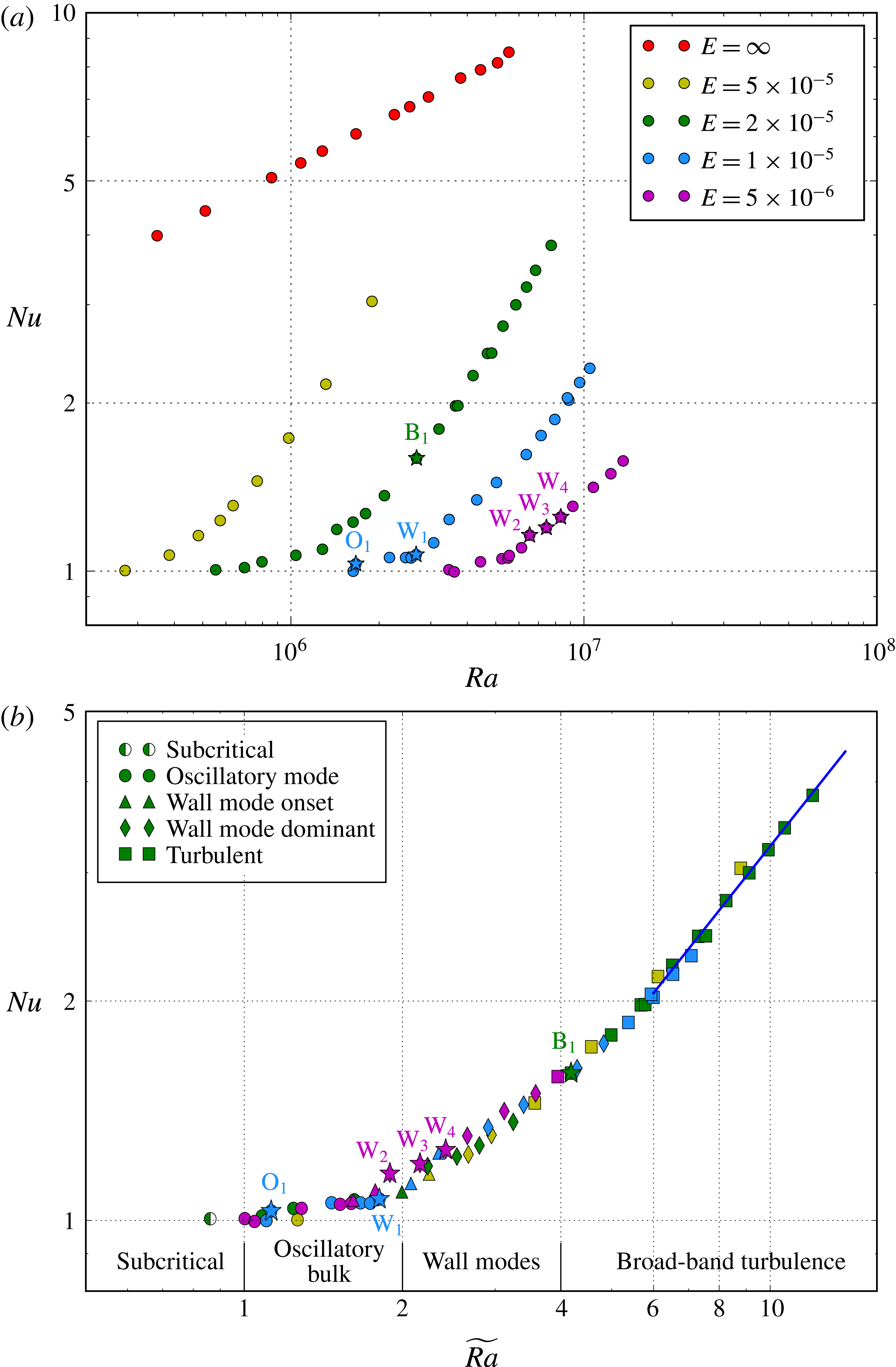
(a) Nusselt number,
 $Nu$
, plotted versus the Rayleigh number,
 $Ra$
, for all the rotating (RC) and non-rotating (RBC) cases. The corresponding Ekman number is indicated with the symbol colour. (b) Nusselt number plotted versus supercriticality
 $\widetilde{Ra}$
for rotating convection. Four main regimes are found: subcritical to convection; oscillatory convection in the fluid bulk; wall-mode-dominated convection; and broad-band turbulence. In the turbulent regime, the best fit is
 $Nu\sim \widetilde{Ra}^{0.9}$
for
 $\widetilde{Ra}\gtrsim 6$
, shown as the blue solid line. The selected cases
 $\text{O}_{1}$
,
 $\text{W}_{1}$
–
 $\text{W}_{4}$
and
 $\text{B}_{1}$
are denoted by star symbols.

The spectral analysis of the preceding section demonstrates that three main regimes of rotating convection exist in the experiments presented here: oscillatory bulk convection, wall-mode-dominated convection and broad-band turbulence. Here we show that these low-
 $Pr$
RC regimes also have decipherably different convective heat transfer signatures.
We first present heat transfer measurements from non-rotating (
 $E=\infty$
) RBC cases. These provide a baseline for comparison with other low-
 $Pr$
RBC studies (e.g. Scheel & Schumacher Reference Scheel and Schumacher2016). In addition, heat transfer in RBC cases approximates the upper bounding values for RC datasets (Cheng et al.
Reference Cheng, Stellmach, Ribeiro, Grannan, King and Aurnou2015; Gastine et al.
Reference Gastine, Wicht and Aubert2016).
The efficiency of heat transfer is expressed non-dimensionally in terms of the Nusselt number,
 $$\begin{eqnarray}\displaystyle & \displaystyle Nu={\displaystyle \frac{Q_{tot}}{Q_{cond}}}={\displaystyle \frac{PH}{k\unicode[STIX]{x0394}TA}}, & \displaystyle\end{eqnarray}$$
which is the ratio of the total vertical heat flux
 $Q_{tot}$
and the conductive flux
 $Q_{cond}=k\unicode[STIX]{x0394}T/H$
.
Figure 6(a) shows
 $Nu$
plotted as a function of
 $Ra$
. The best-fit power law to the
 $E=\infty$
, non-rotating (
 $\text{N}$
) RBC data is
 $$\begin{eqnarray}\displaystyle & \displaystyle Nu_{\text{N}}=(0.151\pm 0.02)\,Ra^{0.256\pm 0.01}. & \displaystyle\end{eqnarray}$$
The value of the power law exponent value is in good agreement with those reported in the laboratory studies of Rossby (Reference Rossby1969) and King & Aurnou (Reference King and Aurnou2013), as well as in the high-resolution
 $Pr=0.021$
direct numerical simulations of Scheel & Schumacher (Reference Scheel and Schumacher2016). However, the coefficient is nearly 20% smaller than the value found in the
 $\unicode[STIX]{x1D6E4}\simeq 1$
study of King & Aurnou (Reference King and Aurnou2013). In addition to aspect ratio (Bailon-Cuba, Emran & Schumacher Reference Bailon-Cuba, Emran and Schumacher2010) and sidewall conductivity differences (e.g. Ahlers Reference Ahlers2000), the coefficient might also be affected by small differences in our material properties parametrisations and in the mean fluid temperature values at a given
 $Ra$
.
Rotating convective heat transfer data are also displayed in figure 6. As expected from (2.11), figure 6(
 $a$
) shows that convective onset occurs at successively higher
 $Ra$
values as the Ekman number decreases. Figure 6(b) shows
 $Nu$
data plotted versus supercriticality
 $\widetilde{Ra}\equiv Ra/Ra_{O}^{cyl}$
. The weakly supercritical data in the range
 $1\lesssim \widetilde{Ra}\lesssim 2$
show a region of relatively weak convective heat transfer in all of the datasets. A regime of weak heat transfer scaling also exists in RBC in metals near onset (Chiffaudel, Fauve & Perrin Reference Chiffaudel, Fauve and Perrin1987; Kek & Müller Reference Kek and Müller1993). However, in low-
 $Pr$
RBC, the weak heat transfer regime arises due to a balance between viscous and weak thermal buoyancy forces. In contrast, in our RC data, this weak heat transfer regime arises because the inertial, oscillatory convection contains no local mean flows that carry thermally anomalous fluid vertically across the layer.
The triangles in figure 6(b) denote cases at, or just after, the onset of sidewall convection, whereas the rhombi denote the cases where the wall modes provide the dominant signature in the temperature spectra. In addition to spectral power, the wall modes also come to dominate the heat transfer at
 $\widetilde{Ra}\gtrsim 2$
, causing a steeper heat transfer scaling. In the frame precessing at the wall mode drift rate, the wall modes drive steady local mean flows across the fluid layer. These mean flows are far more efficient at vertically fluxing heat across the fluid layer than the oscillatory bulk motions that first develop in our experiments.


The square symbols in figure 6(b) denote cases with broad-band temperature spectra, and correspond here to cases with
 $\widetilde{Ra}\gtrsim 4$
. The blue solid line in figure 6(b) shows the best-fit power law,
 $Nu=0.40\,\widetilde{Ra}^{0.91}$
, to all the broad-band data with
 $\widetilde{Ra}\gtrsim 6$
. This scaling differs significantly from the
 $Nu\sim (RaE^{4/3}Pr^{-1/3})^{3/2}\sim \widetilde{Ra}^{3/2}$
scaling that was found in
 $0.3\leqslant Pr\leqslant 1$
fluids (Julien et al.
Reference Julien, Knobloch, Rubio and Vasil2012a
). This
 $Ra^{3/2}$
scaling is argued to hold in the limit of low
 $Ro$
geostrophic turbulence. Our
 $Ra^{0.9}$
scaling differs from the prediction, likely for the following reasons: our data are still too close to onset to exhibit clear asymptotic scalings (e.g. King et al.
Reference King, Soderlund, Christensen, Wicht and Aurnou2010); we are fitting less than a decade of data in terms of supercriticality; and, as shown in figure 7, the global and local convective Rossby numbers are all above
 $0.1$
for the broad-band data and thus unlikely to be in the regime of geostrophically balanced turbulence. Rather, we interpret our broad-band cases as existing in a rotationally dominated, transitional regime.
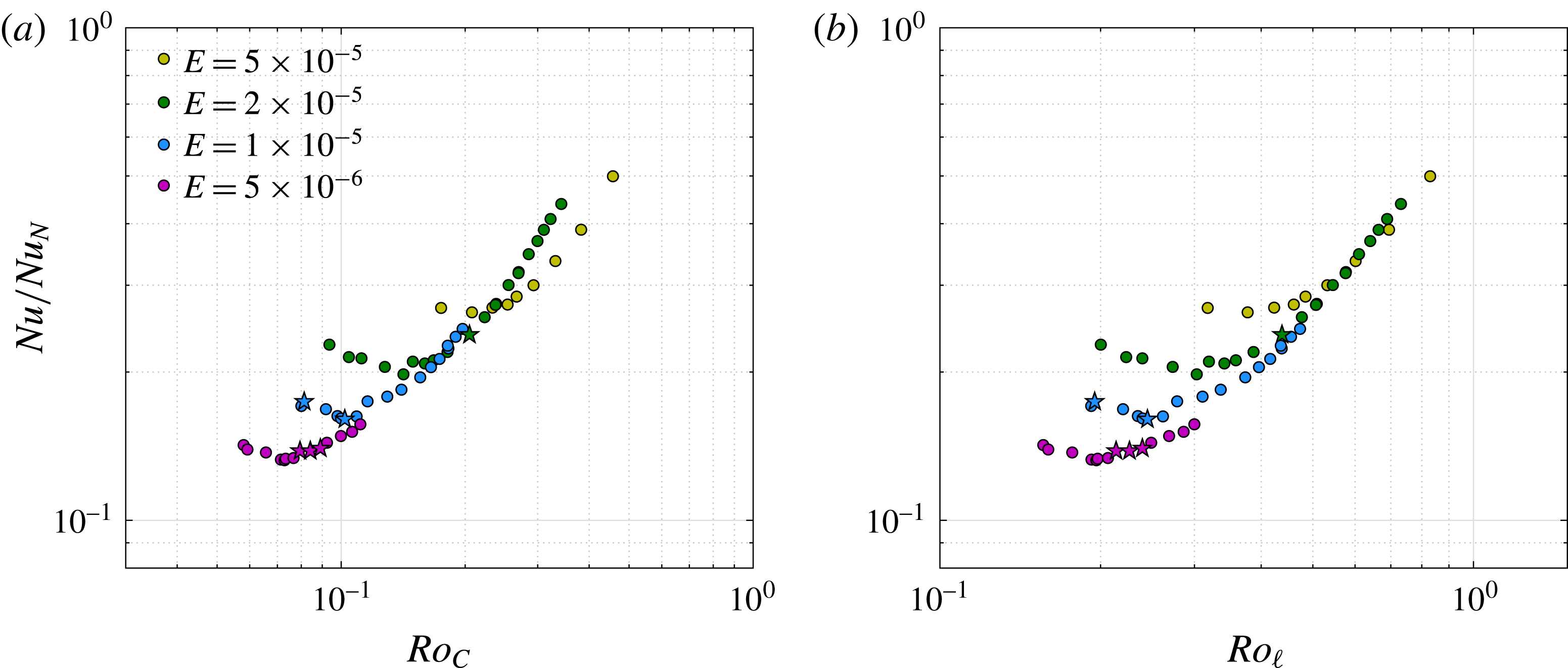
Figure 7 shows rotating heat transfer data normalised by the non-rotating scaling trend,
 $Nu/Nu_{\text{N}}$
. Our present data collapse reasonably well when plotted versus the system-scale convective Rossby number,
 $Ro_{C}$
, displayed in figure 7(a). An equally adequate collapse, perhaps even better for the broad-band heat transfer data, is achieved using the local-scale convective Rossby number
 $Ro_{\ell }$
. This is shown in figure 7(b), where (2.12) is used to estimate the characteristic length scale, yielding
 $$\begin{eqnarray}\displaystyle & \displaystyle Ro_{\ell }=\sqrt{{\displaystyle \frac{\unicode[STIX]{x1D6FC}g\unicode[STIX]{x0394}T}{4\unicode[STIX]{x1D6FA}^{2}H}}{\displaystyle \frac{1}{\ell _{O}^{\infty }}}}=\sqrt{{\displaystyle \frac{RaE^{5/3}}{2.4Pr^{2/3}}}}. & \displaystyle\end{eqnarray}$$
The initial downward sloping in the left portion of each
 $E$
-dataset corresponds to the bulk oscillatory regime of weak heat transfer at
 $1\lesssim \widetilde{Ra}\lesssim 2$
. The slope is negative because the heat transfer scaling exponent in the oscillatory regime is smaller than the RBC scaling exponent in (4.2). The minimum of each
 $E$
-dataset agrees well with the onset of wall modes,
 $\widetilde{Ra}_{W}\simeq 1$
, where the heat transfer efficiency increases. The right-hand branches of the four
 $E$
-datasets collapse for
 $Ro_{\ell }\gtrsim 0.5$
, arguably where the various local-scale convection structures lose their axial coherence. We argue that the local Rossby number maintains its physical meaning at
 $Ro_{\ell }\gtrsim 0.5$
because the horizontal length scale
 $\ell _{O}^{\infty }$
remains intact. This interpretation is based on high-
 $Pr$
rapidly rotating convection, where the horizontal length scale is still characterised by
 $\ell _{S}^{\infty }$
even well after the system-depth columns have broken apart (Julien et al.
Reference Julien, Rubio, Grooms and Knobloch2012b
).
4.3 Bimodal, low-frequency regime
(a–c) Nusselt numbers plotted versus time in thermal diffusion time scale units
 $\unicode[STIX]{x1D70F}_{\unicode[STIX]{x1D705}}$
for cases W
 $_{2}$
,
 $\text{W}_{3}$
and
 $\text{W}_{4}$
carried out at
 $E\simeq 5\times 10^{-6}$
. (d–f) Corresponding temperature spectra obtained through time series from
 $S_{2/3}$
(red) and
 $S_{0}$
(blue). The dashed green (dot-dashed yellow) lines correspond to the onset frequency of the bulk oscillatory mode (wall mode). The dotted purple lines mark the dominant wall mode frequency of case W
 $_{2}$
with
 $\widetilde{f}_{W_{2}}=0.0408$
and
 $\text{W}_{4}$
with
 $\widetilde{f}_{W_{4}}=0.0439$
, as well as the beat frequency in case
 $\text{W}_{3}$
,
 $\widetilde{f}_{beat}=\widetilde{f}_{W_{4}}-\widetilde{f}_{W_{2}}=3.1\times 10^{-3}$
. The solid purple line corresponds to the thermal diffusion frequency
 $\widetilde{f}_{\unicode[STIX]{x1D705}}=2E/Pr=3.8\times 10^{-4}$
.

Spectral peaks of very low frequency can be seen in figure 5, in particular, for case
 $\text{W}_{3}$
, where the maximum PSD occurs at
 $\widetilde{f}\approx 10^{-3}$
. This low-frequency variability hints at the existence of a bimodal or multi-modal flow regime.
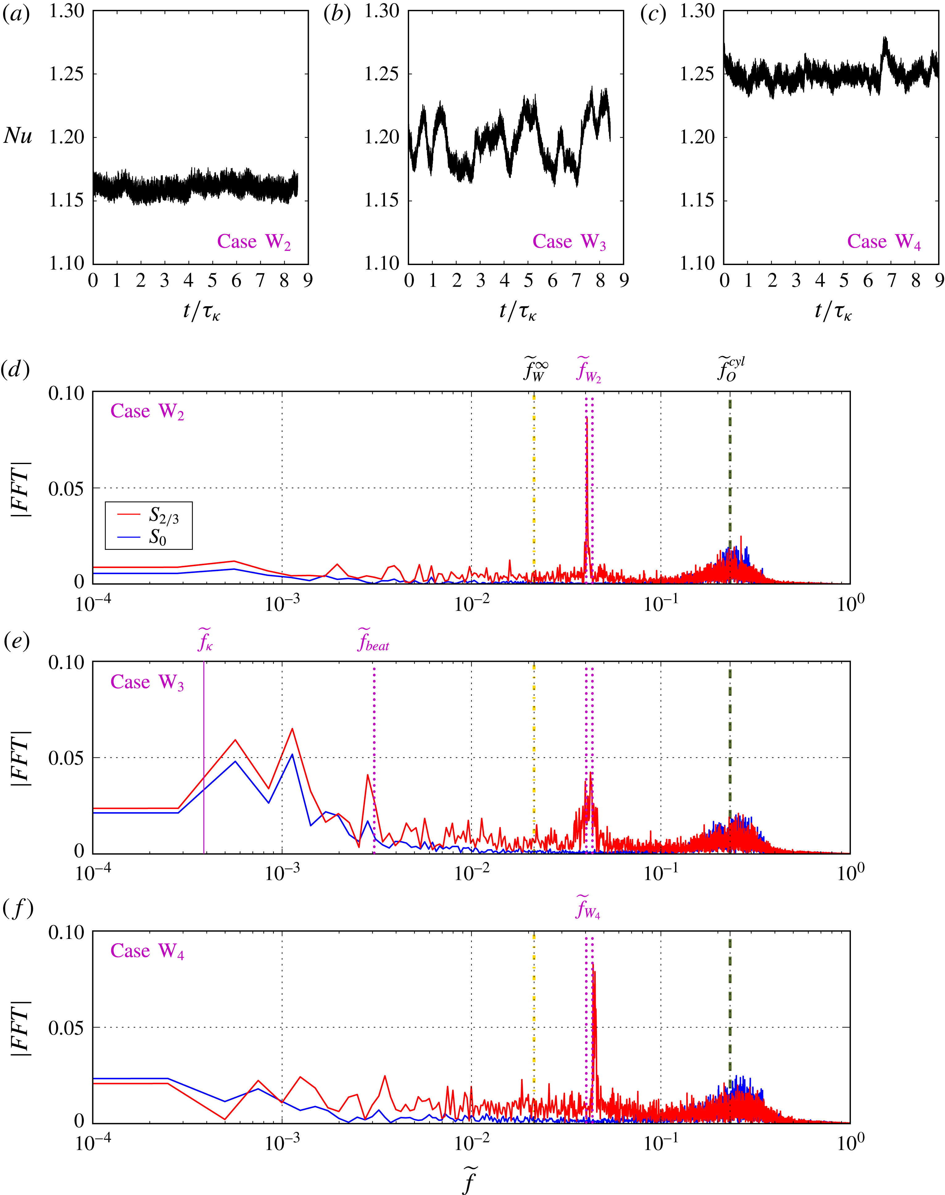
Figures 8(a–c) show Nusselt number time series from cases W
 $_{2}$
,
 $\text{W}_{3}$
and
 $\text{W}_{4}$
, each plotted for roughly nine thermal diffusion time scales,
 $\unicode[STIX]{x1D70F}_{\unicode[STIX]{x1D705}}$
. The rotation rate is the same for these three cases, such that
 $E=5\times 10^{-6}$
. The thermal forcing, and accordingly the supercriticality, is increased successively in steps, from
 $\widetilde{Ra}=1.89$
, to
 $\widetilde{Ra}=2.16$
, to
 $\widetilde{Ra}=2.42$
. The time variations of the Nusselt numbers in cases W
 $_{2}$
and
 $\text{W}_{4}$
occur on the fluctuation time scales of the oscillatory convective flows. In contrast, case
 $\text{W}_{3}$
features larger-amplitude swings in
 $Nu$
occurring on much longer time scales that are closer to
 $\unicode[STIX]{x1D70F}_{\unicode[STIX]{x1D705}}$
.
The respective temperature spectra for the
 $S_{2/3}$
and
 $S_{0}$
thermistor time series are presented in figure 8(d–f). The wall modes for case W
 $_{2}$
and
 $\text{W}_{4}$
have narrow spectral peaks at slightly different frequencies,
 $\widetilde{f}_{W_{2}}=0.0408$
and
 $\widetilde{f}_{W_{4}}=0.0439$
, whereas the wall mode peak of
 $\text{W}_{3}$
is comparatively broad, but with two sub-peaks at
 $\widetilde{f}_{W_{2}}$
and
 $\widetilde{f}_{W_{4}}$
. This observation implies that the
 $\text{W}_{3}$
flow is at least bimodal. We hypothesise that the system transitions via two different metastable modes, and according to figure 8(b), one of these modes more efficiently transfers heat. This agrees with the occurrence of the low-frequency maxima measured by
 $S_{2/3}$
. Estimating that the system remains in each of the states for approximately
 $\unicode[STIX]{x1D70F}_{\unicode[STIX]{x1D705}}$
translates to a thermal diffusion frequency of
 $2\unicode[STIX]{x03C0}f_{\unicode[STIX]{x1D705}}=\unicode[STIX]{x1D70F}_{\unicode[STIX]{x1D705}}^{-1}$
, which yields a normalised frequency value of
 $\widetilde{f}_{\unicode[STIX]{x1D705}}=2E/Pr=3.8\times 10^{-4}$
in this case. Furthermore, we surmise that these modes can also coexist for finite amounts of time. During such times, their interference generates a beat frequency at
 $\widetilde{f}_{beat}=\widetilde{f}_{W_{4}}-\widetilde{f}_{W_{2}}=3.1\times 10^{-3}$
predominantly in the
 $S_{2/3}$
spectrum in figure 8(e).
The explanation of why the two lowest-frequency maxima are obtained by both sensors,
 $S_{2/3}$
and
 $S_{0}$
, is less clear. It suggests that the wall and bulk oscillatory modes couple together and interact nonlinearly. Such a coupling was shown to occur in the low-
 $Pr$
RC cases carried out by Horn & Schmid (Reference Horn and Schmid2017). In addition, these interactions may lead to resonances, such that energy is driven to low frequencies, and possibly to large scales (see Favier, Silvers & Proctor Reference Favier, Silvers and Proctor2014; Plumley et al.
Reference Plumley, Julien, Marti and Stellmach2016). Future experiments will include high-spatial-resolution sidewall sensor arrays in order to better map the complex sidewall dynamics in these experiments.
5 Discussion
Our experimental results demonstrate that different convective modes can co-exist within the same fluid domain in low-
 $Pr$
rotating convection, as predicted by Goldstein et al. (Reference Goldstein, Knobloch, Mercader and Net1994). Convection first onsets via bulk oscillatory modes, in good agreement with the theoretical analysis of Zhang & Liao (Reference Zhang and Liao2009). Wall modes are identified for the first time in liquid gallium, developing in our specific laboratory set-up at
 $\widetilde{Ra}\simeq 2$
. The wall mode frequencies are in adequate agreement with the linear asymptotic analyses of Herrmann & Busse (Reference Herrmann and Busse1993) and Zhang & Liao (Reference Zhang and Liao2009). However, the wall modes in our experiments have lower onset
 $Ra$
values than predicted. The experimental case W
 $_{2}$
(
 $E=5\times 10^{-6},\,\widetilde{Ra}=1.89$
) demonstrates that high-frequency inertial oscillatory modes can dominate the fluid bulk, while lower-frequency wall modes can simultaneously precess around the container’s periphery. Further, a number of cases have low-frequency heat transfer variability that occurs not on inertial time scales, but instead on thermal diffusion time scales. A broad-band, turbulent regime is found at stronger forcings with
 $\widetilde{Ra}\gtrsim 4$
. However, since the global and local convective Rossby numbers are relatively close to unity in the broad-band regime (
 $Ro_{C}\gtrsim 0.1$
and
 $Ro_{\ell }\gtrsim 0.3$
), these cases may not be directly sampling the low-
 $Pr$
quasigeostrophic turbulence regime, but instead are more likely to be characterising a rotationally dominated, transitional regime. In summary, our results illustrate the propensity for multi-modal, scale-separated dynamics in low-
 $Pr$
rotating convection.
We find rather different rotating convective flows in liquid metals in comparison to those that develop in
 $Pr\simeq 1$
models of planetary core dynamics (see Christensen Reference Christensen2011; Jones Reference Jones2011). In particular, no regime with steady columnar convection is found to exist in our liquid metals experiments. This differs from convective flows in current non-metal-based dynamo models, in which a finite regime of quasisteady columns exists that appears to be important for the generation of Earth-like magnetic fields (Sreenivasan Reference Sreenivasan2010; Christensen Reference Christensen2011; Soderlund, King & Aurnou Reference Soderlund, King and Aurnou2012). Similarly, in asymptotically reduced plane-layer models of low-
 $Pr$
rotating convection, oscillatory convection gives way to geostrophic turbulence without ever forming steady columns (for example, see the
 $Ra=Ra_{S}^{\infty }$
,
 $Pr=0.0235$
case in figure 14 of Aurnou et al.
Reference Aurnou, Calkins, Cheng, Julien, King, Nieves, Soderlund and Stellmach2015). Thus, steady convection columns do not form in cylindrical laboratory, low-
 $Pr$
models made at finite
 $E$
, nor do they form in planar models made in the asymptotically reduced, low-
 $E$
, low-
 $Ro$
limit (Julien et al.
Reference Julien, Rubio, Grooms and Knobloch2012b
).
The arguments above implicitly assume that thermal driving dominates the convection occurring in planetary cores. For Earth, this may be a reasonable argument prior to the formation of the solid inner core (see, however, O’Rourke & Stevenson Reference O’Rourke and Stevenson2016). In contrast, we speculate that it may be possible for oscillatory convection to dominate the local-scale, thermocompositional convection occurring in the present-day Earth. Since
 $Ra_{O}^{\infty }\sim 10^{-2}Ra_{S}^{\infty }$
, it is plausible that thermally driven oscillatory flows will develop more easily and destabilise compositionally driven quasisteady flows, even if the compositional buoyancy forcing exceeds the thermal forcing. Alternatively, the admixture of these two buoyancy sources may directly drive broad-band quasigeostrophic convective turbulence.
We note though that caution must be exercised in mapping our cylindrical results to planetary, spherical shell geometries. In lower to middle latitudes outside the tangent cylinder, spiralling convective flows are the onset behaviour for Earth-like
 $Pr$
(Kaplan et al.
Reference Kaplan, Schaeffer, Vidal and Cardin2017; Zhang & Liao Reference Zhang and Liao2017). Convection within the tangent cylinder develops only at higher
 $Ra$
values, beyond the reach of linear stability analyses. Strongly nonlinear models of high-latitude, thermocompositional convection must be developed that use realistic diffusivity values for the dynamically active components in order to address these zeroth-order dynamical questions. This point seems especially relevant, given the outsized influence that tangent cylinder flows seem to exert in global-scale dynamo generation processes and on the magnetic field morphology in a variety of models (e.g. Glatzmaier & Roberts Reference Glatzmaier and Roberts1995; Aubert et al.
Reference Aubert, Aurnou and Wicht2008; Schaeffer et al.
Reference Schaeffer, Jault, Nataf and Fournier2017).
Lastly, our experimental results demonstrate that wave modes naturally develop adjacent to the container’s boundary, even in a fully convective fluid layer. Thus, our liquid metal laboratory results appear to support scenarios in which planetary dynamo action is driven by multi-modal turbulent convective flows, whilst the secular variation of the magnetic field is controlled by the dynamics of slow, larger-scale, wave modes localised near the core–mantle boundary (e.g. Finlay & Jackson Reference Finlay and Jackson2003; Jaupart & Buffett Reference Jaupart and Buffett2017).
Acknowledgements
Authors are listed in alphabetical order to reflect equally distributed contributions. We thank the four anonymous referees for constructive feedback that greatly improved this paper. This work was supported by the NSF Geophysics Program, award no. 1547269. V.B. acknowledges École Normale Supérieure de Paris for funding his internship in Los Angeles. S.H. acknowledges funding by the Deutsche Forschungsgemeinschaft (DFG) under grant HO 5890/1-1. T.V. acknowledges the Helmholtz Association for their financial support.
Appendix A. Material properties of gallium
A.1 Viscosity
The viscosity of liquid gallium is difficult to measure precisely for a number of reasons, including its affinity to oxygen. As soon as liquid gallium comes in contact with the atmosphere, gallium oxides form on its free surface and then populate the bulk fluid. These oxides can affect the measurement of the viscosity. To minimise this phenomenon, our entire experimental system is flushed with argon. Following Brito et al. (Reference Brito, Nataf, Cardin, Aubert and Masson2001), we cycle our 99.99 %-purity liquid gallium through a 5 % hydrochloric acid solution before filling the tank (e.g. https://www.youtube.com/watch?v=G1qwMHkboDY).
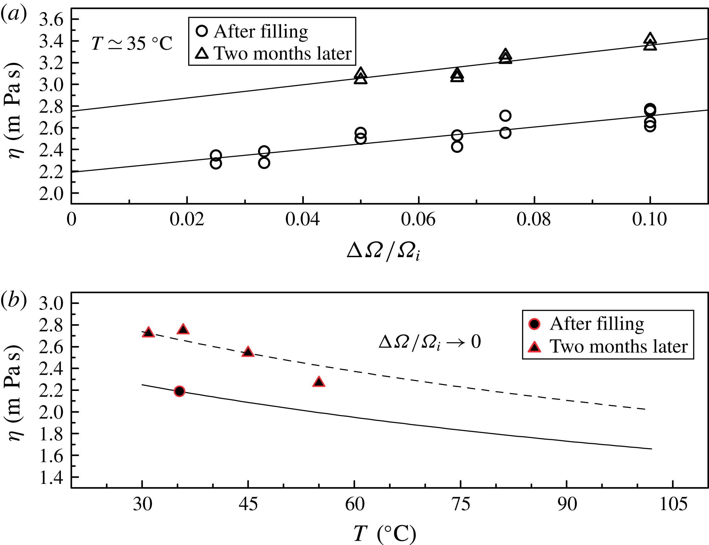
In situ dynamic viscosity estimates made from spin-up experiments. (a) Estimates for fluid at
 $T\simeq 35~^{\circ }\text{C}$
as a function of spin-up amplitude
 $\unicode[STIX]{x0394}\unicode[STIX]{x1D6FA}/\unicode[STIX]{x1D6FA}_{i}.$
The hollow circles (triangles) denote data acquired roughly 1 week (2 months) after the container was filled with gallium. (b) Viscosity extrapolations to zero forcing amplitude at different fluid temperatures.

Even under well-controlled conditions, however, measurements of liquid gallium’s dynamic viscosity,
 $\unicode[STIX]{x1D702}=\unicode[STIX]{x1D70C}\unicode[STIX]{x1D708}$
, vary by as much 40 % between differing studies (Spells Reference Spells1936; Grosse Reference Grosse1961; Genrikh et al.
Reference Genrikh, Kaplun and Solovev1972; Iida et al.
Reference Iida, Morita and Takeuchi1975; Brandes & Brook Reference Brandes and Brook1992; Iida, Guthrie & Tripathi Reference Iida, Guthrie and Tripathi2006; Assael et al.
Reference Assael, Armyra, Brillo, Stankus, Wu and Wakeham2012; Xu et al.
Reference Xu, Oudalov, Guo, Jaeger and Brown2012). To address this issue, we have carried out an independent set of experiments in which we use acoustic Doppler velocimetry to measure linear spin-up in our tank of gallium under nearly isothermal conditions (see Brito et al.
Reference Brito, Aurnou and Cardin2004). In these experiments, the tank is spun up in less than 1 s (fixed
 $4~\text{r.p.m.}~\text{s}^{-1}$
ramp) from an initial rotation rate
 $\unicode[STIX]{x1D6FA}_{i}$
to
 $\unicode[STIX]{x1D6FA}_{i}+\unicode[STIX]{x0394}\unicode[STIX]{x1D6FA}$
. Azimuthal velocity,
 $u_{\unicode[STIX]{x1D719}}$
, measurements are made along a midplane chord (inset, figure 3). The velocity data are averaged around the midpoint of the chord, which is located 73 mm to 77 mm from the ultrasonic transducer and at a radial position
 $r_{m}\simeq 0.70R_{i}$
.
Figure 3 shows normalised Doppler velocity measurements,
 $u_{\unicode[STIX]{x1D719}}/\unicode[STIX]{x0394}\unicode[STIX]{x1D6FA}r_{m}$
, versus time shifted relative to
 $t_{o}$
, the instant of peak measured velocity. The fluid temperature is
 $T=35.8~^{\circ }\text{C}$
here and the spin-up goes from 40.0 r.p.m. to 44.0 r.p.m. (
 $\unicode[STIX]{x0394}\unicode[STIX]{x1D6FA}/\unicode[STIX]{x1D6FA}_{i}=0.1$
). The fluid responds via an exponential temporal adjustment to the new solid-body rotation rate. This occurs on the spin-up time scale
 $$\begin{eqnarray}\displaystyle & \displaystyle \unicode[STIX]{x1D70F}_{su}=(8E)^{-1/2}\,\unicode[STIX]{x1D6FA}_{i}^{-1}=H/(2\sqrt{\unicode[STIX]{x1D708}\unicode[STIX]{x1D6FA}_{i}}) & \displaystyle\end{eqnarray}$$
(Greenspan & Howard Reference Greenspan and Howard1963; Greenspan Reference Greenspan1969; Warn-Varnas et al.
Reference Warn-Varnas, Fowlis, Piacsek and Lee1978). We estimate
 $\unicode[STIX]{x1D70F}_{su}$
here as the time at which the
 $u_{\unicode[STIX]{x1D719}}/\unicode[STIX]{x0394}\unicode[STIX]{x1D6FA}r_{m}=\exp (-1)$
. From
 $\unicode[STIX]{x1D70F}_{su}$
, the kinematic viscosity is found by recasting (3.1) as
 $$\begin{eqnarray}\displaystyle & \displaystyle \unicode[STIX]{x1D702}=\unicode[STIX]{x1D70C}H^{2}/(4\unicode[STIX]{x1D6FA}_{i}\unicode[STIX]{x1D70F}_{su}^{2}). & \displaystyle\end{eqnarray}$$
Figure 9(a) shows spin-up measurements of
 $\unicode[STIX]{x1D702}$
for fluid at
 $T\simeq 35~^{\circ }\text{C}$
and for a range of
 $\unicode[STIX]{x1D6FA}_{i}$
and
 $\unicode[STIX]{x0394}\unicode[STIX]{x1D6FA}/\unicode[STIX]{x1D6FA}_{i}$
values. The hollow circles correspond to spin-up measurements acquired the same week that we filled the tank with cleaned gallium. The hollow triangles correspond to measurements made two months later. The fluid viscosity increases over this two-month time window. This is caused by the existence of an intermetallic phase that develops on the tank’s horizontal boundaries. Although relatively thin (
 ${\lesssim}1~\text{mm}$
thick), this heterogeneous layer increases the mechanical coupling relative to the initially smooth walls present at the time of the fill. This layer does not, however, change the bulk properties of the fluid; heat transfer measurements were repeatable over the two-month time window for RBC cases made with the same input heating.
For each suite of experiments made at a fixed time, the viscosity estimates in figure 9(a) increase with increasing spin-up amplitude
 $\unicode[STIX]{x0394}\unicode[STIX]{x1D6FA}/\unicode[STIX]{x1D6FA}_{i}$
. We account for this by linearly extrapolating the viscosity data to
 $\unicode[STIX]{x0394}\unicode[STIX]{x1D6FA}/\unicode[STIX]{x1D6FA}_{i}=0$
(filled symbols with red outlines). These extrapolated values, which we take to be working viscosity of the fluid, are plotted in figure 9(b). Four different temperatures were measured two months after the tank was filled, whereas measurements were only made at near
 $35~^{\circ }\text{C}$
just after the tank was filled.
We best fit our gallium viscosity data as a function of temperature using the Andrade (Reference Andrade1934) formulation,
 $$\begin{eqnarray}\displaystyle & \displaystyle \unicode[STIX]{x1D702}=\unicode[STIX]{x1D702}_{0}\,\exp \left({\displaystyle \frac{E_{a}}{R\,T}}\right), & \displaystyle\end{eqnarray}$$
where the activation energy is
 $E_{a}=4000~\text{J}~\text{mol}^{-1}$
and the gas constant is
 $R=8.3144~\text{J}~(\text{mol}~\text{K})^{-1}$
. This functional form was first employed by Grosse (Reference Grosse1961) to fit the gallium viscosity data of Spells (Reference Spells1936), and has been used widely since (Brandes & Brook Reference Brandes and Brook1992; Braunsfurth et al.
Reference Braunsfurth, Skeldon, Juel, Mullin and Riley1997; King & Aurnou Reference King and Aurnou2013). We argue here that our ‘two-month’ data are fitted reasonably well by (3.2) with a viscosity coefficient of
 $\unicode[STIX]{x1D702}_{o}=0.56~\text{mPa}~\text{s}$
(dashed line in figure 9
b). However, we believe the
 $T=35~^{\circ }\text{C}$
data acquired just after filling the tank more accurately characterise the bulk viscosity of the fluid. The data yield a viscosity coefficient value of
 $\unicode[STIX]{x1D702}_{0}=0.46~\text{mPa}~\text{s}$
(solid line in figure 9(b), in adequate agreement with the values of Spells Reference Spells1936; Iida et al.
Reference Iida, Morita and Takeuchi1975; Brandes & Brook Reference Brandes and Brook1992; King & Aurnou Reference King and Aurnou2013. Thus, we use
 $\unicode[STIX]{x1D702}_{0}=0.46~\text{mPa}~\text{s}$
in (3.2) in all the ensuing viscosity estimates employed in this study.
Vertical temperature difference,
 $\unicode[STIX]{x0394}T$
, measured versus the input power,
 $P$
, for the four thermal conduction experiments realised. The dashed blue line shows the best linear fit
 $\unicode[STIX]{x0394}T=0.1079~\text{K}~\text{W}^{-1}\,P-0.067~\text{K}$
.

A.2 Thermal conductivity
In cases with relatively high rotation rate and low thermal forcing, the fluid is convectively stable and the heat transferred across the gallium conductively. These conduction cases allow us to make in situ measurements of the thermal conductivity,
 $k$
, of the gallium within our convection device. Figure 10 shows the temperature difference between the top and the bottom of the tank,
 $\unicode[STIX]{x0394}T$
(K), plotted versus the input power,
 $P$
(W), for the four conduction cases carried out. The dashed line is a linear regression
 $\unicode[STIX]{x0394}T=\unicode[STIX]{x1D6FD}P+b$
. In conjunction with Fourier’s law of conduction, the value of the slope,
 $\unicode[STIX]{x1D6FD}=0.1079~\text{K}~\text{W}^{-1}$
, gives a thermal conductivity value
 $$\begin{eqnarray}\displaystyle & \displaystyle k=H/(\unicode[STIX]{x03C0}R_{i}^{2}\,\unicode[STIX]{x1D6FD})=(31.4\pm 0.1)~\text{W}~(\text{m}~\text{K})^{-1}, & \displaystyle\end{eqnarray}$$
where
 $R_{i}=D/2=0.09~\text{m}$
is the inner radius of the acrylic cylinder. The coefficient of determination of this linear fit is
 $R^{2}=0.9999$
. Further, the intercept of the linear regression,
 $b=-0.067~\text{K}$
, is close to zero and is small compared to the temperature differences in these conduction cases (
 ${\lesssim}1\,\%$
). This suggests that our thermal conductivity measurement is relatively accurate. In addition, it agrees well with other, independent laboratory estimations (Aurnou & Olson Reference Aurnou and Olson2001; King & Aurnou Reference King and Aurnou2013).
Parameters used for the conduction measurements of the thermal conductivity of liquid gallium: temperature difference
 $\unicode[STIX]{x0394}T$
across the tank; mean fluid temperature
 $\overline{T}$
; power input
 $P$
to the heat pad; angular rotation rate
 $\unicode[STIX]{x1D6FA}$
, Rayleigh number
 $Ra$
and supercriticality
 $\widetilde{Ra}$
. The heat flux is equal to the power divided by the area of the tank,
 $(\unicode[STIX]{x03C0}D^{2})/4$
, with
 $D=0.194~\text{m}$
.
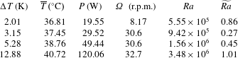
Appendix B. Convection data
Parameters for the conducted laboratory experiments. The first four columns show the derived non-dimensional control parameters: Ekman number
 $E$
, Rayleigh number
 $Ra$
, Prandtl number
 $Pr$
and supercriticality
 $\widetilde{Ra}\equiv Ra/Ra_{O}^{cyl}$
. The next four columns show the measured dimensional control parameter: angular rotation rate
 $\unicode[STIX]{x1D6FA}$
, applied heating power
 $P$
, vertical temperature difference
 $\unicode[STIX]{x0394}T$
and mean fluid temperature
 $\overline{T}$
. The second to last column gives the Nusselt number
 $Nu$
. The last column indicates the respective regime for every case. N stands for non-rotating convection, S for subcritical, O for oscillatory convection, W for wall-localised convection, and B for broad-band turbulence. The selected bold cases are discussed in detail throughout this study.