1.1. Introduction

People swiftly began researching the inertial confinement fusion using a high power laser, but after more than 50 years, we are finally on the verge of a milestone. The National Ignition Facility at Lawrence Livermore National Laboratory is now delivering its full potential of 4.2 MJ and it will be the first machine on earth that will achieve a controlled ignition of fusion (Moses, Reference Moses2009). On the other hand, for practical inertial fusion energy, there is a race on increasing the output energy of high repetition rate laser (Zheng et al., Reference Zheng, Zhang, Wei, Jing, Sui, Zheng, Yuan, Jiang, Su, Zhou, Li, Wang, Hu, He, Xiang, Peng, Feng, Guo, Li, Zhu, Yu, You, Fan and Zhang2008; Albach et al., Reference Albach, Arzakantsyan, Bourdet, Chanteloup, Hollander and Vincent2008; Chanteloup et al., Reference Chanteloup, Albach, Lucianetti, Ertel, Banerjee, Mason, Hernandez-Gomez, Collier, Hein, Wolf, Körner and Le Garrec2010). Inertial fusion is not the only objective of lasers with high power and high repetition rate. There are many research fields that utilizes the high power and high repetition rate laser such as laser acceleration of particles, high energy density states of matter, laser induced plasma generation, X-ray and extreme ultraviolet generation (Batanov et al., Reference Batanov, Goncharov and Min'ko1972; Tajima & Dawson, Reference Tajima and Dawson1979; Jin & Richardson, Reference Jin and Richardson1995; Salamin et al., Reference Salamin, Hu, Hatsagortsyan and Keitel2006). There are also many applications in industry such as laser processing of materials, laser peening, next generation lithography using extreme ultraviolet, and medical lasers (Spalding, Reference Spalding1978; Masse & Barreau, Reference Masse and Barreau1995; Sumiyoshi et al., Reference Sumiyoshi, Sekita, Arai, Sato, Ishihara and Kikuchi1999; Salamin et al., Reference Salamin, Harman and Keitel2008).

To increase the output energy of a laser while maintaining its repetition rate, researchers tried many techniques. They researched on laser materials (cryogenic Yb:YAG and ceramic Nd:YAG), pumping methods (laser diode pumping), and advanced laser schemes (beam combining, fiber laser) (Zhou et al., Reference Zhou, Kane, Dixon and Byer1985; Barnes et al., Reference Barnes, Storm, Cross and Skolaut1990; Kong et al., Reference Kong, Lee, Shin, Byun, Park and Kim1997; Ikesue, Reference Ikesue2002; Limpert et al., Reference Limpert, Deguil-Robin, Manek-Hönninger, Salin, Röser, Liem, Schreiber, Nolte, Zellmer, Tünnermann, Broeng, Petersson and Jakobsen2005; Lee et al., Reference Lee, Choi, Kim and Zhou2007; Kawanaka et al., Reference Kawanaka, Takeuchi, Yoshida, Pearce, Yasuhara, Kawashima and Kan2010). Among these, the most practical solution for the laser fusion driver is the beam combination laser using stimulated Brillouin scattering-phase conjugate mirror (SBS-PCM) due to its unlimited scalability without thermal problems (Kong et al., Reference Kong, Lee, Shin, Byun, Park and Kim1997, Reference Kong, Lee and Lee2005b, Reference Kong, Lee and Lee2005c, Reference Kong, Lee, Lee and Guo2005d). Like other beam combination techniques, it can be operated with a high repetition rate over 10 Hz since only small amplifiers are needed to obtain the high output energy. Also, SBS-PCM can compensate a wavefront distortion automatically and removes a need of complicated and expensive deformable mirrors (Rockwell, Reference Rockwell1988). Finally, the self-phase locking of SBS-PCM enables the separate phase controlling/locking of each beam lines (Kong et al., Reference Kong, Lee, Shin, Byun, Park and Kim1997, Reference Kong, Lee and Lee2005b, Reference Kong, Lee, Lee and Guo2005d); thereby the number of beams can be increased without limit in the number of beams.

In this work, we introduce key concepts of the beam combination laser using the SBS-PCM with necessary experiments. After that, we present four beam combining results, both with and without amplifiers. Recent progresses on a prepulse technique of the SBS-PCM will also be showed.

1.2. Progresses and Experimental Results

1.2.1. Beam Combination Laser Using Self-Phase Controlled SBS-PCM

The self-phase controlling/locking of SBS-PCM is the most important feature of the coherent beam combination laser using SBS-PCM. Since a phase conjugate wave of the normal SBS-PCM is originated from an acoustic noise in the medium, it has a random phase with respect to a phase of the input beam (Rockwell, Reference Rockwell1988; Boyd et al., Reference Boyd, Rzazewski and Narum1990). Figure 1 shows the schemes of the self-phase locking. Feedback mirror is installed at the back side of the SBS-PCM and the interference between the original beam and the returning beam makes an optical standing wave at the focus. The optical standing wave ignites and generates a moving Bragg grating by electrostriction at the right moment. The phase conjugate wave of the self-phase controlled SBS-PCM is originated from this moving Bragg grating and has a definite phase. It is proved that the self-phase controlling/locking of SBS-PCM effectively locks and controls the phase of the SBS wave with a very simple optical configuration (Kong et al., Reference Kong, Lee, Shin, Byun, Park and Kim1997).

Fig. 1.

(Color online) The proposed scheme of the self-phase controlling method. Counter-propagation beams from the feedback mirror and incident beams make a standing density modulation in the SBS-medium. Standing density modulation locks the ignition position of moving Bragg grating, and the Bragg grating locks the phase of the SBS-wave.

Figures 2 and 3 shows the proposed scheme of the coherent beam combination laser using SBS-PCMs with the wavefront dividing and the amplitude dividing schemes, respectively. Cross-type feature of the scheme is treated heavily in a previous review (Kong et al., Reference Kong, Yoon, Beak, Shin, Lee and Lee2007a) and we will concentrate on the amplifier arm in this work.

Fig. 2.

(Color online) The experimental setup of the beam-combined laser system with the wavefront dividing scheme. The beam is divided by prisms. PBS = polarized beam splitter; FR = Faraday rotator; Amp = amplifier; Q = quarter wave plate.

Fig. 3.

(Color online) The experimental setup of the beam-combined laser system with the amplitude dividing scheme. The beam is divided by PBSs. PBS = polarized beam splitter; FR = Faraday rotator; Amp = amplifier; Q = quarter wave plate.

When a beam enters the beam combination amplifier stage, it is separated into several sub-beams. In the wavefront dividing scheme, the input beam is divided spatially by an apertures and prisms. In the amplitude dividing scheme, the input beam is divided energetically by wave-plates and polarizing beam splitters (PBSs). Each of the sub-beams passes through an amplifier and a Faraday rotator. The Faraday rotator not only rotates the polarization of the beam, but also compensates thermal depolarization induced by the amplifier in the double pass configuration (Han & Kong, Reference Han and Kong1995). Finally, sub-beams are combined into the output beam coherently.

1.2.1.1. Compensation of Thermal Depolarization

Thermally induced birefringence (TIB) is one of the most significant thermal effects seen in the amplifiers. It is known that among four configurations given in Figure 4, only Figure 4d would completely compensate depolarization effect by TIB with a 90° rotated polarization (Han & Kong, Reference Han and Kong1995).

Fig. 4.

(Color online) Experimental setup for the measurement of the leak beam patterns and the depolarization ratio for the four possible optical schemes in a double-pass Nd:YAG rod amplifier with a SBS-PCM (W = wedged window; EM1 and EM2 = energy meters; PBS = polarizing beam splitter; QWP = quarter wave plate; AMP = Nd:YAG rod amplifier; FR = Faraday rotator; L = lens). (a) QWP-AMP (quarter wave plate located before the amplifier), (b) AMP-QWP (quarter wave plate located after the amplifier), (c) FR-AMP (Faraday rotator located after the amplifier), (d) AMP-FR (Faraday rotator located before the amplifier).

Figure 4 shows the experimental setup for the measurement of the leak beam patterns and the depolarization ratios using the four possible optical schemes in a double-pass Nd:YAG amplifier with an SBS-PCM (Shin et al., Reference Shin, Park and Kong2010a). The laser beam from the 1064 nm pulsed Nd:YAG oscillator has a quasi-Gaussian shape with a beam diameter of 8 mm. This beam is double-pass amplified using the four possible schemes with the help of an SBS-PCM as a reflector. The electrical input energy to the pumping flashlamp is adjustable from 0 to 37.5 J. After the laser amplification, small depolarized part of the output beam passes through the PBS with a p-polarization. An optical wedge is located before the PBS and reflects a small amount of the beam. An energy meter measures the energy and a charge coupled device camera measures the beam pattern.

Figure 5 shows the depolarization ratios versus the electrical input energy for the four different optical schemes. Figure 5 also shows the theoretical fits from the Jones matrix calculation with a Faraday rotation angle of 44.3°. Figure 6 shows the theoretically and experimentally obtained leak beam patterns when the electrical input energy is 30.4 J. The theoretical leak beam patterns are obtained from the Jones matrix calculations and the fitted value. The results show a good agreement between the theoretical and experimental results.

Fig. 5.

(Color online) Experimental data and theoretical fits of the depolarization ratios versus the electrical input energy to the Xenon flashlamp for the four different optical schemes. (a) QWP-AMP, (b) AMP-QWP, (c) FR-AMP, (d) AMP-FR.

Fig. 6.

Theoretically and experimentally obtained leak beam patterns for the four possible optical schemes when the electrical input energy to the Xenon flashlamp is 30.4 J. (a) QWP-AMP, (b) AMP-QWP, (c) FR-AMP, (d) AMP-FR.

1.2.1.2. Feedback Control of Long-Term Phase Fluctuation

Due to the air fluctuations and other effects, lengths of the sub-beam paths are varying in long term. It can be seen as slowly changing relative phase between the beams. A typical time scale is much larger than the period of the laser pulses (0.1 s).

To solve this long-term problem, we actively control the beam path lengths using piezoelectric translator (PZT) (Kong et al., Reference Kong, Yoon, Shin, Beak and Lee2006, Reference Kong, Yoon, Shin and Beak2008). At first, the relative phases between the beams are measured from the interference pattern between the sub-beams or by measuring the relative polarization components of the combined beam. Using the measured relative phases, the position of the feedback mirror is adjusted by applying the feedback voltages to the attached PZTs. Note that the process is done between the pulses. Therefore expensive real-time modules are unnecessary. The control of long-term phase fluctuation extends the period of phase locking from less than a minute to an hour or more.

1.2.1.3. Two Beam Combination Laser — Wavefront Dividing Scheme

Figure 7 shows the experimental setup of the two beam combination laser with the wavefront dividing scheme. The laser beam is expanded by a beam expander, which consists of a pair of lenses. The beam is expanded four times and passes through the aperture. The aperture divides the beam into two beams. Two beams pass through the PBS, and one beam line is reflected from the prism and the mirror to the SBS-PCM. Another beam propagates through the PBS and the Faraday rotator. Two beams are reflected from the SBS-PCMs, and the reflected beams are split by the wedges. The length of the SBS cell is 300 mm, and the radius of curvature of the feedback convex mirror is 300 mm. The charge-coupled device camera detects the interference pattern of the two beams and calculates the relative phase to make the input voltage into the PZT controller. The PZT controller adjusts the position of the feedback mirror with the PZT.

Fig. 7.

(Color online) The experimental setup for the long-term phase stabilization assessment in the wavefront dividing scheme. PBS = polarizing beam splitter; M = mirror; W = wedged window; FR = Faraday rotator; CM = concave mirror; PZT = piezoelectric translator.

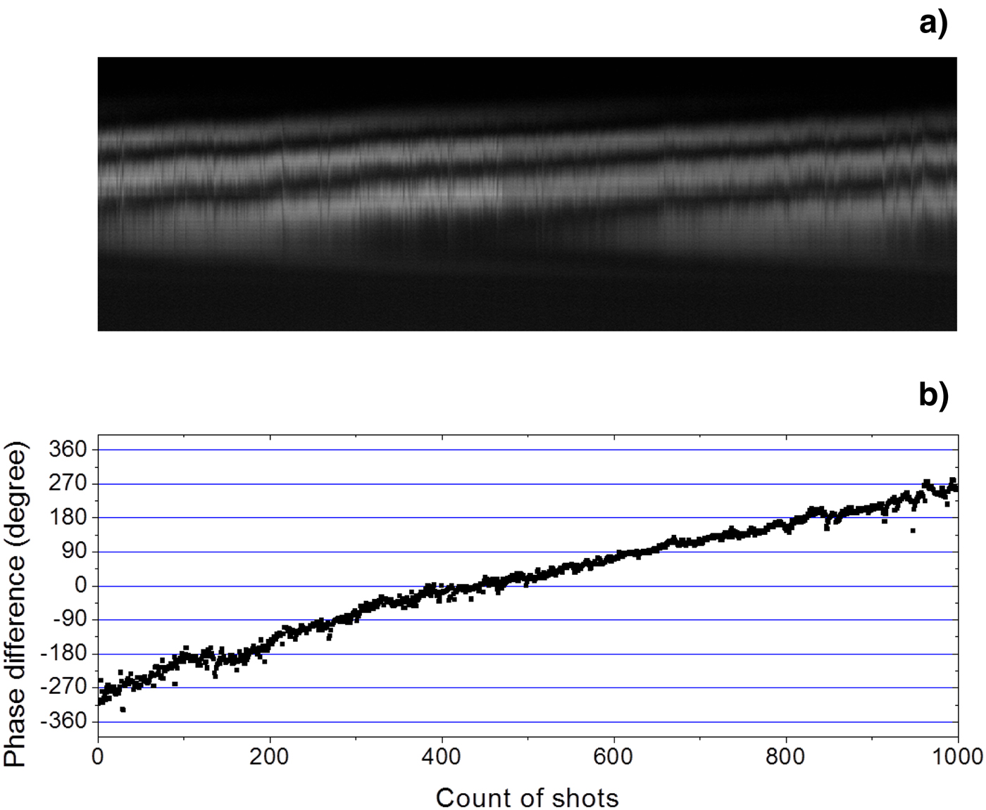
Without the long-term phase control, Figure 8 shows the relative phase and the output energy measured during 1000 shots (100 s). It shows the slow varying relative phase and the output energy. With the long-term phase control, Figure 9 shows the relative phase and the output energy measured during 1000 shots (250 s). The phase fluctuation is λ/28.8 in standard deviation, and the output energy is stabilized near its maximum value.

Fig. 8.

The experimental results of the wavefront dividing two-beam combination without long-term phase stabilization. (a) Mosaic intensity profile of the horizontal lines from interference patterns during 1000 shots. (b) The phase difference during 1000 shots.

Fig. 9.

(Color online) The experimental results of the wavefront dividing two-beam combination with long-term phase stabilization. (a) Mosaic intensity profile of the horizontal lines from interference patterns during 1000 shots. (b) The phase difference during 1000 shots. The standard deviation of the phase difference is λ/28.8.

1.2.1.4. Two Beam Combination Laser — Amplitude Dividing Scheme

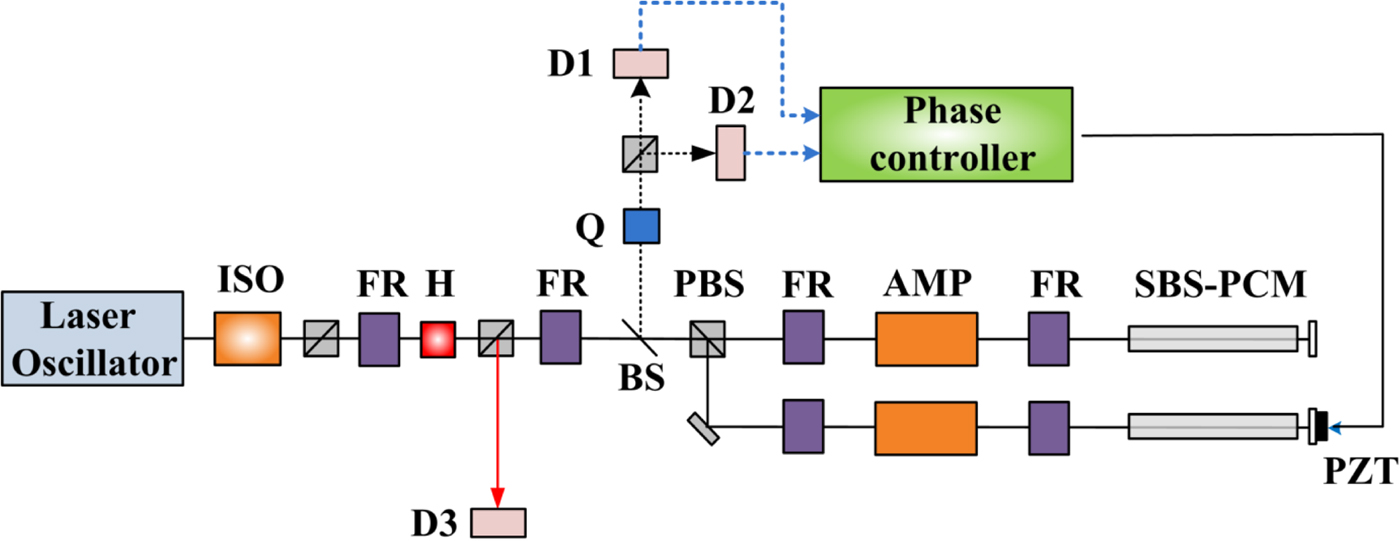
Figure 10 shows the experimental setup of the two beam combination laser with the amplitude dividing scheme. The laser beam passes through the isolator, the PBS, the Faraday rotators, the half wave plate (HWP). After that, the beam propagates through the PBS, the FR, and the BS. The beam is split into two beams by the PBS and reflected from the SBS-PCMs. The reflected beam is split by the BS, passes through the quarter wave plate (QWP), and is split into two beams again by the PBS. The divided beams are measured in terms of their energy by the detectors, D1 and D2.

Fig. 10.

(Color online) The experimental setup of the long-term phase stabilization assessment with the amplitude dividing scheme without amplifiers. ISO = isolator; FR = Faraday rotator; H = half wave plate; Q = Quarter wave plate; BS = Beam splitter; PBS = Polarized beam splitter; D1-D3 = Detector.

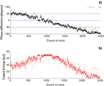
Without the long-term phase control, Figure 11 shows the relative phase and the output energy measured during 2500 shots (250 s). It shows the slowly varying relative phase and the output energy. With the long-term phase control, Figure 12 shows the relative phase and the output energy measured during 2500 shots (250 s). The phase fluctuation is λ/46.7 in standard deviation, and the output energy is stabilized near its maximum value.

Fig. 11.

(Color online) The experimental results of the amplitude dividing two-beam combination without long-term phase stabilization. (a) Phase difference during 2500 shots. (b) Output energy during 2500 shots.

Fig. 12.

(Color online) The experimental results of the amplitude dividing two-beam combination with long-term phase stabilization. (a) Phase difference during 2500 shots. The standard deviation of the phase difference is λ/46.7. (b) Output energy during 2500 shots. Maximum energy is 80.9 mJ, and median energy is 77.1 mJ, Mean energy is 76.3 mJ.

Figure 13 shows the experimental setup in which the Faraday rotators and the amplifiers are added to Figure 10. This setup is designed to investigate the coherent beam combination characteristics during the laser amplification process. Figure 14 shows the result with the PZT control during 2500 shots (250 s). The phase fluctuation is λ/22.5 and the standard deviation of the output energy is 7.18%.

Fig. 13.

(Color online) The experimental setup of the long-term phase stabilization assessment with the amplitude dividing scheme with amplifiers. ISO = isolator; FR = Faraday rotator; AMP = amplifier; H = half wave plate; Q = Quarter wave plate; BS = Beam splitter; PBS = Polarized beam splitter; D1-D3 = Detector; PZT = piezoelectric transducer.

Fig. 14.

(Color online) The experimental results of the amplitude dividing two-beam combination with long-term phase stabilization. (a) Phase difference during 2500 shots. The standard deviation of the phase difference is λ/22.5. (b) Output energy during 2500 shots. Maximum energy is 228 mJ, and median energy is 211 mJ, Mean energy is 208 mJ.

1.2.2. Coherent Four Beam Combination Laser Using SBS-PCM

Two beam coherent combination lasers can represent the scalability that is one of the most important features of the beam combination laser using SBS-PCM. Moreover, the relative phase between the two sub-beams can be measured by using simple interferogram between the beams. On the other hand, four beam combination lasers can also show that it can be expanded to have more sub beams by successive splitting of the input laser beam. Also, the phase measurement methods can be applied to more complex beam combination systems.

1.2.2.1. Four Beam Combination Laser Amplifier — Wavefront Dividing Scheme

A four-beam combined laser with the wavefront dividing scheme was successfully demonstrated both with and without amplifiers (Kong et al., Reference Kong, Shin, Yoon and Beak2009b; Shin et al., Reference Shin, Park, Kong and Yoon2010b). Figure 15 shows the experimental setup of the four-beam combined laser with the wavefront dividing scheme. A beam expander expands the size of the laser beam by four times and a four-circular aperture shapes the laser beam into the four circular beams. After passing through PBS1, the beam is split spatially by three prisms, P1, P2, and P3. Four beams are named beam 1, beam 2, beam 3, and beam 4. Each sub-beam passes through the amplifiers and the Faraday rotators. At the end of each beam line, the self-phase controlled SBS-PCM reflects the beam. Combined output beam is reflected from the PBS1.

Fig. 15.

(Color online) The experimental setup of the wavefront dividing four-beam combined laser. PB1 and PBS2 = polarizing beam splitters; HWP1 and HWP2 = half wave plate; P1, P2, and P3 = 45° prisms; BS = beam splitter; W = wedged window; FR1, FR2, FR3, and FR4 = Faraday rotators; C1, C2, C3, and C4 = concave mirrors; PZT1, PZT2, and PZT3 = piezoelectric transducers.

To measure the relative phase differences between sub-beams, an optical wedge reflects a part of beam 1. We will name it beam 0. On the other hand, using HWP2, a small amount of the output beam passes through PBS2. This part of the output beam forms an interference pattern with the expanded beam 0. The relative phases are measured from the interferogram, and the phase controlling electronics controls the PZTs.

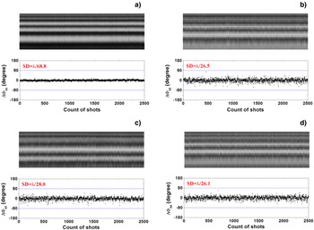
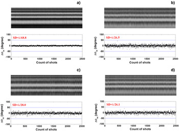
Figure 16 shows the output beam profiles and the interferograms. Figure 17 shows the measured phase distributions of each sub-beams without amplifiers, and Figure 18 show the measured phase distributions of each sub-beams with amplifiers. When the amplifiers are not operating, the input energy is 32.2 mJ ± 0.3 mJ and the output energy is 9.9 mJ ± 0.5 mJ. The standard deviation of the phase difference between beam 0 and the four parts of output beam are measured to be λ/86.2, λ/36.3, λ/35.8, and λ/43.4. When the amplifiers are operating, the input energy is 32.2 mJ ± 0.3 mJ and the output energy is increased to be 169 mJ ±6 mJ. The standard deviation of the phase difference between the beam 0 and the four parts of output beam are determined to be λ/68.8, λ/26.5, λ/28.0, and λ/26.1.

Fig. 16.

(Color online) The experimental results of the beam profile and interferograms. (a) The output beam profile. (b) The interferograms. The large beam profile, noticed by red arrow, is the reference beam.

Fig. 17.

(Color online) The mosaic intensity profile of the horizontal lines from interference patterns and phase difference of the wavefront dividing four-beam combined laser without amplifiers. (a) for ΔΦ01, (b) for ΔΦ02, (c) for ΔΦ03, and (d) for ΔΦ04.

Fig. 18.

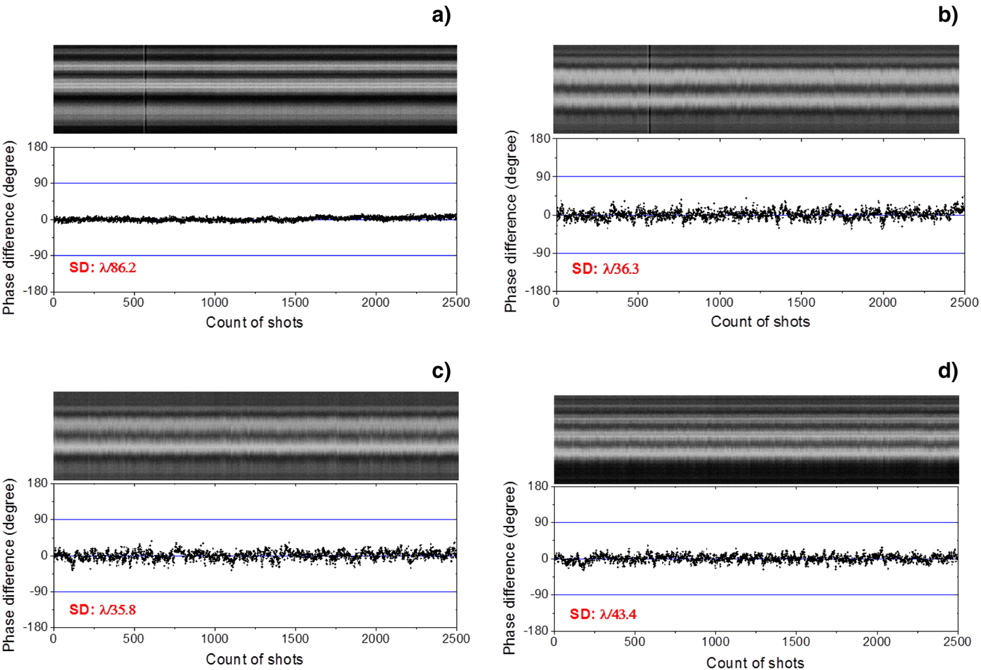
(Color online) The mosaic intensity profile of the horizontal lines from interference patterns and phase difference of the wavefront dividing Four-beam combined laser with amplifiers. (a) for ΔΦ01, (b) for ΔΦ02, (c) for ΔΦ03, and (d) for ΔΦ04.

1.2.2.2. Four Beam Combination Laser Amplifier — Amplitude Dividing Scheme

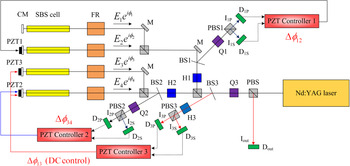
A four-beam combined laser with the amplitude dividing scheme was successfully demonstrated (Kong et al., Reference Kong, Shin, Yoon and Beak2009a). Figure 19 shows the experimental setup of the four-beam combined laser with the amplitude dividing scheme. After passing through the PBS, QWP changes the polarization of the laser beam from p-polarization to circular polarization. Another PBS splits the beam into two sub-beams. For each beam, the polarization is rotated 45° by PBS. Finally, two more PBS split sub-beams into four sub-beams. At the end of each beam line, the self-phase controlled SBS-PCM reflects the beam. Combined output beam is reflected from the first PBS.

Fig. 19.

(Color online) The experimental setup of the amplitude dividing four-beam combined laser. PB1 = polarized beam splitter; HWP1 and HWP2 = half wave plate; QWP = quarter wave plate; BS1, BS2, and BS3 = beam splitters; CM = concave mirror; PZT1, PZT2, and PZT3 = piezoelectric transducers.

To measure the relative phase differences between sub-beams, beam splitters reflect a part of combining beams. BS1 and BS2 reflect a part of the two beam combined outputs. From the reflected beams of BS1 and BS2, the relative phases between two beams are measured. BS3 reflects a part of the four beam combined output. From the reflected beam of BS3, the relative phase between the two two-beam combined beams is measured. The phase controllers control the PZTs.

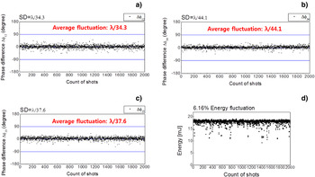
Figure 20 shows the measured phase differences between the beams. Figures 20a and 20b shows the measured phase differences between the two beams and Figure 20c shows the measured phase differences between two-beam combined beams. The standard deviations of the phase differences are λ/34.3, λ/44.1, and λ/37.6. The fluctuation of the output energy is 6.16%.

Fig. 20.

(Color online) The phase difference of the amplitude dividing four-beam combined laser without amplifiers for 2500 shots and energy distribution for 2500 shots. (a) for ΔΦ12, (b) for ΔΦ34, (c) for ΔΦ13, and (d) Energy distribution for 2500 shots.

1.2.3. Recent Progresses on the Prepulse Technique

It is known that the front part of reflected pulse from SBS-PCM is consumed to generate the moving Bragg grating (Kong et al., Reference Kong, Beak, Lee and Lee2005a; Reference Kong, Lee and Lee2005c). To preserve the waveform of the pulse, the prepulse technique is suggested and demonstrated (Kong et al., Reference Kong, Beak, Lee and Lee2005a; Beak et al., Reference Beak, Yoon, Shin and Kong2008; Yoon et al., Reference Yoon, Shin, Kong and Lee2009). In the prepulse technique, an input pulse is split into the prepulse and the main pulse. The prepulse has energy of about the threshold energy of the SBS-PCM. The prepulse arrives at the SBS-PCM earlier and ignites a moving Bragg grating. The front part of the main pulse is highly reflected by the preformed moving grating and the waveform of the reflected pulse is preserved.

1.2.3.1. Relationship Between the Optimum Prepulse Energy and the Delay Time for the Waveform Preservation

Figure 21 shows the experimental setup for measuring the waveforms of SBS waves with varying prepulse energy levels and delay time. An input pulse has a pulse width of 7–8 ns and a repetition rate of 10 Hz. After passing through an optical isolator, the input beam passes through HP2 and is divided by PBS2 into two sub-beams — the main pulse and the prepulse. The main pulse energy is fixed at 10 mJ. The main pulse is reflected by PBS4 and passes the delay line twice. A quarter wave plate (QP) in the delay line rotates the polarization of the main pulse by 90°, so the main pulse passes through the PBS4. HP3 and PBS3 play the role of adjusting the prepulse energy. HP4 and HP5 and the Faraday rotators (FR1 and FR2) rotate the polarization by −45° and 45°, respectively, and thus the main pulse with p-polarization and the prepulse with s-polarization are combined at PBS5 with some time delay. Finally, both pulses enter the SBS-PCM. The focal length of the focusing lens is 15 cm. The reflected prepulse retraces the path of the incident prepulse beam and is dumped out at PBS3 because its polarization is changed by HP4 and FR1. By the same reason, the reflected main pulse is reflected by PBS4 and photodiode (PD) measures the waveform of the main pulse. The signal from the PD was measured by an oscilloscope operating with a bandwidth of 500 MHz and a sampling rate of 500 Msamples/s.

Fig. 21.

Experimental setup for the prepulse injection method. HPs = half-wave plates; PBSs = polarizing beam splitters; ISO = optical isolator; FRs = Faraday rotators; QP = quarter-wave plate; M = mirror; L = focusing lens; PD = photodiode.

Figure 22 shows the temporal waveforms measured at a delay time of 15 ns. As the prepulse energy increases, the waveform of the reflected pulse becomes more similar to that of the input pulse. When the prepulse energy is more than 2 mJ, the pulse shape is perfectly preserved. Figure 23 shows the simulation and the experimental results of the minimum prepulse energies required to preserve the waveform over the prepulse delay time. The simulation result is obtained by calculating the energy stored in the acoustic grating at the time of the main pulse arrival. From the experimental result, we can conclude that the optimum prepulse delay time is 15 ns and the required prepulse energy at this delay is 2 mJ per pulse.

Fig. 22.

Reflected waveforms when td = 15 ns: (a) E _pre= 0 mJ, (b) E _pre= 1.5 mJ, (c) E _pre= 1.8 mJ, and (d) E_pre >>  2 mJ.

Fig. 23.

Required prepulse energy versus the delay time [the experimental results (filled dots) and the simulation results (blank dots)].

2.1. Introduction

The stimulated Brillouin scattering (SBS) in various solids, liquids, and gases is a very powerful tool to build the phase conjugation mirror (PCM) in high-power laser systems (Rockwell, Reference Rockwell1988; Dane et al., Reference Dane, Neuman and Hackel1994a; Yoshida et al., Reference Yoshida, Kmetik, Fujita, Nakatsuka, T. Yamanaka and Yoshida1997, Reference Yoshida, Fujita, Nakatsuka and Yoshida1999, Reference Yoshida, Fujita, Nakatsuka, Fujinoki and Yoshida2003, Reference Yoshida, Fujita, Nakatsuka and Fujinoki2004; Kong et al., Reference Kong, Lee and Lee2005b, Reference Kong, Lee and Lee2005c, Reference Kong, Yoon, Shin, Beak and Lee2006, Reference Kong, Yoon, Beak, Shin, Lee and Lee2007a; Meister et al., Reference Meister, Riesbeck and Eichler2007; Kappe et al., Reference Kappe, Strasser and Ostermeyer2007; Yasuhara et al., Reference Yasuhara, Kawashima, Sekine, Kurita, Ikegawa, Matsumoto, Miyamoto, Kan, Yoshida, Kawanaka, Nakatsuka, Miyanaga, Izawa and Kanabe2008). A PCM based on the SBS process can be successfully used to compensate thermally induced phase distortion in high power laser systems. A PCM is very efficient for enhancing the laser beam quality especially in designing a double pass laser amplifier systems. Also, the SBS process can be applied for the high-efficiency pulse compression of an energetic laser pulse.

The SBS compression of laser pulse has been investigated theoretically and experimentally for various laser wavelengths and active SBS media (Dane et al., Reference Dane, Neuman and Hackel1994a; Schiemann et al., Reference Schiemann, Ubachs and Hogervorst1997; Kmetik et al., Reference Kmetik, Fiedorowics, Andreev, Witte, Daido, Fujita, Nakatsuka and Yamanaka1998). The SBS compressor provides enhancement of peak intensity of pulses while maintaining its high energy, and make available laser pulse duration of a few 100 ps. It is difficult to generate mode-locking pulses without damage at high peak power. On the other hand, this method of short-pulse generation is very simple and can be used to achieve high brightness. The heavy fluorocarbon satisfies the demands for SBS medium in the view of excellent optical quality, low absorption in wide spectral region from ultraviolet to infrared, a high threshold of optical breakdown, good thermodynamic properties, and desirable chemical stability. We previously reported that a 8 ns Nd:YAG laser pulse was temporally compressed to a SBS phase conjugation pulse of 600 ps using a 1.7-m-long cell FC-75 liquid (Mitra et al., Reference Mitra, Yoshida, Fujita and Nakatsuka2006). A 13-ns Nd:YAG laser pulse was temporally compressed to about 160-ps phase-conjugated pulse in heavy fluorocarbon FC-40 liquid at a 1064 nm wavelength (Yoshida et al., Reference Yoshida, Hataeh, Fujita, Nakatsuka and Kitamura2010). We are developing a high-average-power short pulse laser system based on optical parametric chirped pulse amplifier (OPCPA) technique. A few hundred ps 532-nm pulse laser will be used to pump the OPCPA system.

For the first time to our knowledge, we demonstrated the efficient compression of 10 ns pulse duration to 160 ps or less at second harmonics of an Nd:YAG laser. The compressed pulse brightness is about 56-fold higher than that of the incident pulse. The heavy fluorocarbon liquid can also be used as phase conjugators for high-average-power.

2.2. Experimental Results

The experimental layout of temporal SBS compression is shown in Figure 24. The laser used was a linearly polarized Q-switched Nd:YAG oscillator at single-frequency and TEM₀₀ mode operation. The amplified output was 10 ns pulse of approximately 500 mJ at a 10 Hz repetition rate. The beam quality was 1.5 times diffraction-limited. The 1064-nm output beam is externally doubled to 532 nm with a KTiOPO₄ (KTP) crystal. KTP was chosen as the nonlinear crystal because of its high effective nonlinear coefficient. The laser light was focused into a SBS cell through a variable attenuator using a combination of a half-wave plate and a thin-film polarizer. The reflected laser beam was separated using a dielectric thin-film polarizer and a quarter-wave plate.

Fig. 24.

The experimental layout of temporal SBS compression.

We have fabricated a long cell for liquid phase conjugation mirror of length 1.5 m and diameter 4 cm. Windows of the cell had antireflection coating at 532 nm. These cells were filled up with FC-40 liquid. Before filling we filter the liquid by using Millipore filters of pore size 0.020 µm. This filtering was important to increase the optical breakdown threshold. The circularly polarized laser beam was focused inside the cell by a lens with focal length of 500 or 1000 mm. The absorption coefficient of FC-40 liquid at 532 nm wavelength was about 1 × 10⁻⁵ cm⁻¹. Experiments on SBS compression were performed using a combined generator-amplifier system. The circularly polarized laser beam was transmitted through the 1.5-m long SBS cell, and was focused into the other 1.5-m long generator using a lens of focal length 750 mm. The pulse shapes of the pump and reflected beams were monitored using a Hamamatsu R1328U-51 biplanar phototube (rise time; 55 ps) and a Tektronix CSA7404 signal analyzer (analog bandwidth; 4 GHz and rise time; 100 ps). The reflected energy was directly measured with a power meter. The SBS backward reflectivity from the FC liquid was also compared with the total reflection from a conventional thin-film mirror (R = 99.5%).

The SBS gain coefficient was independent of the pumping wavelength in the transparent medium. The FC-40 was reported to be 2 cm/GW at 1064 nm. The phonon lifetime τ_B and Brillouin bandwidth Δν_B depend inversely on the pump wavelength assuming that τ_B ∝ λ_p⁻² and Δν_B = 1/2π τ_B. The phonon lifetime τ_B is proportional to λ_p⁻², so that τ_B at 1064 nm is one-fourth that at 532 nm. FC-40 liquid with a fast SBS relaxation time was selected from a lot of heavy fluorocarbon. The τ_B value at 1064 and 532 nm for FC-40 were approximately 250 and 70 ps, respectively.

Because SBS begins from a leading edge of the propagating pulse, an optimum reflection is expected for a spatial length of the pulse, (c/2n) τ_π, where τ_π is the pulse width (full width at half maximum (FWHM)) and n is the refractive index of a FC liquid. For a 10 ns pulse and a refractive index n = 1.28, the interaction length L _in was taken as 117 cm. The optical path length of the Brillouin cell, L = 150 cm was chosen over 117 cm to satisfy the condition L > L _in.

The SBS compression reflectivity for several focal lengths in a FC-40 liquid is shown in Figure 25. A maximum intrinsic SBS reflectivity of over 90% was obtained at incident energy of over 100 mJ. The SBS threshold of about 5 mJ was observed. On the other hand, the Brillouin generator-amplifier system that consist of L = 1500 mm amplifier and f = 750 mm generator was obtained a maximum SBS reflectivity of 35% at an incident energy of about 200 mJ. This system controls the energy entering the Brillouin generator to prevent optical breakdown. A SBS reflectivity using f = 1000 mm lens was slightly lower than that using f = 500 mm lens. It confirms that the SBS process can be effective if the coherence length of the optical pulse is equal to or longer than the length of the Stokes field region. In practice, it denotes that the coherence length of the SBS pump pulse should be longer than the confocal length of the focused SBS pump beam divided by a refractive index. The bandwidth of the laser oscillator used here is 250 MHz and so that the coherence length L _c is about 120 cm. The interaction length L in the SBS material using f = 500 nm or = 1000 mm was 64 cm and 128 cm, respectively. In the case of the 500-mm-focal-length lens, a condition L _c > L was satisfied; however, in the case of the 1000-mm-focal-length lens, this condition was marginal.

Fig. 25.

SBS reflectivity measured at 532 nm pumping.

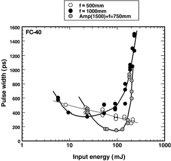
The SBS compressed-pulse duration using several different focal lengths is shown in Figure 26. In the case of the 500-mm focal length, the compressed pulse width was 250 ps at incident energy of 200 mJ. The maximum compression ratio is about 40-fold higher than that of the incident pulse of 10 ns. In the case of the 1000-mm focal length, the minimum pulse width of 350 ps was obtained at 30 mJ input energy, but the compressed pulse width slowly increased. The pulse width at incident energy of 200 mJ was increases in length of 1.5 ns. The Stokes pulse duration depends on the pumping energy, and the compressed minimum pulse width of the Brillouin generator-amplifier system at over 100 mJ reached 160 ps or less. However, the Stokes pulse showed substantially wider pulses as the incident energy increased to 200 mJ. This results from the leading edge of the amplifier Stocks incident pulse interacting with the low energy leading edge of the Gaussian pumping pulse.

Fig. 26.

The compressed pulse duration measured at 532 nm pumping.

The typical shapes of compressed pulses are shown in Figure 27. A slow falling time of the compressed pulse was observed owing to the reduced intensity in the peripheral part of the spatial profile. The pump beam was highly compressed at the center of the beam, while the compression effects were much less at the wings. The pulse shape of the reflected beam was a mixed pulse that combines a fast rising time at the center and a slow falling time at the wing of the pulse. The SBS compressed-pulse duration using a focal length of 500 mm observed the dumping waveform for falling edge because the interaction length of 63 cm is shorter than the necessary length of L = 117 cm. In a focal length of 1000 mm and two cell method, the compressed pulse shape consist of a steep leading edge and a sharp falling edge because the interaction length of the Brillouin cell was about 117 cm. The experimental observations of phase jumps and amplitude fluctuations in SBS were reported (Afshaavahid et al., Reference Afshaavahid, Devrelis and Munch1998) No special pulse compression geometric conditions such as short focal length have an affect on the length of the Stokes-pump interaction. The noise of SBS process results in the fluctuation in the Stokes pulse due to energy interchange between Stokes and pump pulses. The damping time corresponds to the SBS phonon lifetime.

Fig. 27.

The oscilloscope traces of the typical incident and reflected waveforms at several focal length.

The fluctuation of the pulse width greatly depends on the focusing condition of the SBS generator. Figure 28 shows the time fluctuation of input pulses and SBS compression pulses. The jitter timing of SBS compression pulses was about 500 ps and similar to that of the incident Q switched. The focusing condition depends on the input beam quality of shot to shot and the environmental condition of SBS amplifier. The focusing ability of SBS generator decreases with the vibration in the enclosed liquid and the convection flow by an environmental temperature. The SBS phase-conjugation ability corrected these perturbations, but it is necessary the SBS cell have good insulation for focusing condition of the SBS generator.

Fig. 28.

The time fluctuation of input pulses and SBS compression pulses.

In this experiment on pulse compression in FC-40, there is a possibility that the process of stimulated Raman scattering (SRS) competes with SBS. At maximum input energy SRS is weak and does not influence SBS. The nonlinear effects, such as self-phase modulation and self-focusing, were not observed because the nonlinear refractive index (1 × 10⁻⁷ cm²GW⁻¹) of Fluorinert liquid is too low and the beam quality of SBS compression pulse is similar to that of the incident pulse. It will be necessary to measure a nonlinear effect in the future.

3.1. Introduction

High-peak-power high energy pulse lasers of hundreds picoseconds play an important role in the fields of inertial confinement fusion (ICF) (Kong et al., 2005, Reference Kong, Yoon, Beak, Shin, Lee and Lee2007a), diagnostics of plasma by means of Thompson scattering (Mao et al., Reference Mao, Zhao, Li, Xie, Fang, Sannikov and Gorshkov2001) and produce of X-ray radiation for lithography (Endo, Reference Endo2004). Especially in the field of ICF, shock ignition is a new concept for direct-drive laser ICF that was proposed by Betti et al. (Reference Betti, Zhou, Anderson, Perkins, Theobald and Solodov2007). Compared with the standard direct drive central ignition and fast ignition, shock ignition presents overwhelming advantages (McCrory et al., Reference McCrory, Meyerhofer, Betti, Craxton, Delettrez, Edgell, Glebov, Goncharov, Harding, Jacobs-Perkins, Knauer, Mars Hall, Mckenty, Radha, Regan, Sangster, Seka, Short, Skupsky, Smalyuk, Soures, Stoeckl, Yaakobi, Shvarts, Frenje, Li, Petrasso and Séguin2008). It does not require any complex cone-in-a-shell targets or high power chirp pulse amplifier lasers. However, it is a key difficulty to obtain the high-energy and high-power laser pulse with a hundred picoseconds width in the ICF laser driver to achieve shock ignition. Stimulated Brillouin scattering (SBS) is a particularly useful tool to compress a long pulse because of its power compatibility (Wang et al., Reference Wang, Lu, Li, Wu, Zheng and He2010), high energy reflectivity and high compression ratio (Yoshida et al., Reference Yoshida, Hatae, Fujita, Nakatsuka and Kitamura2009). Applied SBS pulse compressor and amplifiers to the high-energy laser system is an efficient way to obtain high intensity picosecond pulses. In this work, we have demonstrated high-energy laser pulse compression and amplification by SBS using a two-cell scheme. A higher energy experiment will be demonstrated in the one-hundred-joule Nd: phosphate glass laser system (Ostermeyer et al., Reference Ostermeyer, Kong, Kovalev, Harrison, Fotiadi, Megret, Kalal, Slezak, Yoon, Shin, Beak, Lee, Lu, Wang, Lin, Knight, Kotova, Straber, Scheikhobeid, Riesbeck, Meister, Eichler, Wang, He, Yoshida, Fujita, Nakatsuka, Hatae, Park, Lim, Omatsu, Nawata, Shiba, Antipov, Kuznetsov and Zakharov2008) in the future.

3.2. Experimental Setup and Design

The experimental setup is shown in Figure 29. A short Stokes seed pulse is obtained by a two-cell SBS generator and then amplified in the Brillouin amplifier.

Fig. 29.

(Color online) Optical layout of SBS temporal-pulse compressor and amplifier.

The laser used in the experiments was a linearly polarized single frequency Q-switched Nd:YAG oscillator (PRII9010, Continuum Inc.) with 8 ns pulse duration and 6 mm beam diameter. The pulse was split by the polarized plate P2. One pulse was seeded into the two-cell generator to produce the Stokes seed pulse. And the other pulse was used as the pump pulse. A compact SBS generator-amplifier setup was used as the picoseconds Stokes generator. In the generator, Lens 1 was a long focal lens (1000–1500 mm) and Lens 2 was a short focal lens (300–500 mm). The length of generating cell 1 and generating cell 2 were 800 mm and 1000 mm, respectively. In the amplifier, the pump pulse propagated through the amplifying cell before the Stokes seed was reflected by M3 and then encountered with the Stokes seed in the amplifying cell. The amplified Stokes pulse was exported by the polarized plate P3. To achieve optimal amplifying result, the encounter time was changed by moving the high reflected mirror M3. The pulse shapes were monitored using a Tektronix DPO7254 oscilloscope (bandwidth 2.5 GHz) and a fiber coupled ultrahigh speed photo detector (18.5 ps, New Focus).

3.3. Experimental Results and Discussion

FC-72 was chosen as the SBS medium in the experiment. The length of the cells and the focal length of Lens 1 were fixed. And the focal length of Lens 2 was set as 300 mm, 600 mm, and 750 mm, respectively. Figure 30 shows the compressed pulse duration changing as the input intensity increasing.

Fig. 30.

(Color online) The results of compact SBS generator-amplifier pulse compression with different focal length of Lens 2: (a) f2 = 300 mm, (b) f2 = 600 mm, (c) f2 = 750 mm.

SBS is a nonlinear process and so the compressed pulse duration is not changing linearly as increasing the input intensity. For different focal length of Lens 2, the stability of compressed pulse duration changes obviously. With shortening of the focal length of Lens 2, the compressed pulse width is becoming increasingly unstable. When the focal length of Lens 2 is 750 mm, the compressed pulse duration is stable at about 1ns with the input intensity 20–40 MW/cm². When the focal length of Lens 2 is 600 mm, the compressed pulse duration is stable with the input intensity 20–30 MW/cm². When the focal length of Lens 2 shortens to 300 mm, the compressed pulse duration is not stable at any input intensity in the experiment.

The energy reflectivity with different focal length of Lens 2 is shown in Figure 31. It is effective to improve the energy reflectivity by lengthening the focal length of Lens 2. The optimal pulse width of compressed pulse and the highest energy reflectivity occurs at different pump intensity. The highest energy reflectivity is nearly 80% in the experiment.

Fig. 31.

The energy reflectivity of different focal length of Lens 2 in compact SBS generator-amplifier scheme: (a) f2 = 300 mm, (b) f2 = 600 mm, (c) f2 = 750 mm.

It is very difficult to achieve sub-nanosecond pulse by changing focal length of Lens 2 with FC-72 because the phonon lifetime of FC-72 is 1.2 ns. We choose several media that have a shorter phonon time as the SBS medium in the generator cell 2. They are HS260 (phonon lifetime: 0.1 ns), FC-43 (phonon lifetime: 0.2 ns) and DET (phonon lifetime: 0.7 ns). The result was shown in Figure 32. In the experiment, the focal length of Lens 2 was fixed at 300 mm. The optimal compressed pulse duration is 760 ps with DET, 490 ps with FC-43 and 312 ps with HS260.

Fig. 32.

(Color online) The pulse compression result with different medium: (a) HS260, (b) DET, (c) FC-43.

The energy reflectivity of our experiment is shown in Figure 33. The energy reflectivity is unstable and is not high with DET and HS260. The energy reflectivity with FC-43 is higher than the other two media and can achieve 80%. The reason is that the gain coefficient of FC-43 is higher and the Stokes shift of FC-43 is close to the Stokes shift of FC-42. In the generating cell 1, a Stokes seed with short duration is excitated by a shorter phonon lifetime medium and in the generating cell 2 the Stokes seed is amplified efficiently by another higher gain medium.

Fig. 33.

The energy reflectivity of the compact SBS generator-amplifier with different medium: (a) HS260, (b) DET, (c) FC-43.

In a word, to achieve a Stokes pulse with 200 ps pulse duration, we should choose the appropriate media of the cell1 and cell 2. Meanwhile, a reasonable compressor structure is important so that the compressor will operate in an optimal condition.

The amplification of the Stokes seed with hundreds picoseconds pulse duration was investigated in the experiment. As a seed, the duration of the Stokes pulse is stabilized at 0.5 ns. FC-72 is selected as the amplifying medium. The length of the amplification cell is 800 mm and 1500 mm. The energy amplification ratio η is defined as

where E _amplified is the energy of amplified Stokes seed in the amplifying cell, E _seed is the energy of Stokes that output from the generating cell and E _pump is the pump energy.

The result of the experiment is shown in Figure 34. The energy amplification ratio is decreasing with the pump intensity increasing. The reason is that the duration of the pump pulse is 8 ns much longer than the Stokes seed with duration of 0.5 ns and the encounter length of the two pulses is not optimal in the experiment. Meanwhile, it was observed that the pulse duration of the amplified Stokes seed was broadened significantly. The results indicated that the pump pulse was not depleted completely by the Stokes seed. In the future the ratio of the pump duration and the Stokes duration and the amplification scheme should be optimized to enhance the conversion efficiency.

Fig. 34.

The energy amplification ratio with different length of the amplification cell: (a) L = 800 mm, (b) L = 1500 mm.

ACKNOWLEDGMENT

This work was supported by the National Natural Science Foundation of China (Grant No. 61008005), the China Postdoctoral Science Foundation (Grant No. 20090450966), Special Foundation (Grant No. 201003428), the Heilongjiang Postdoctoral Science Foundation (Grant No. LBH-Z09128), Natural Scientific Research Innovation Foundation in Harbin Institute of Technology (Grant No. HIT. NSRIF. 2009010), and the Fundamental Research Funds for the Central Universities (Grant No. HIT. KLOF. 2010037).

ACKNOWLEDGMENTS

This work was supported by the International Atomic Energy Agency (IAEA) as a part of the coordinated research project “Pathway to Energy from Inertial Fusion – An Integrated Approach” (Research Contracts No. 13781 and 13758); by the Ministry of Education, Youth, and Sports of the Czech Republic Research Project LC528 and by the grant KONTAKT No. ME933; by the Czech Technical University in Prague grant No.: CTU0916314; and by the Grant Agency of the Czech Republic grant No. 202/08/H057. It was also supported by the Nuclear Research and Development Program of the Korea Science and Engineering Foundation (KOSEF) grant funded by the Korean Government (MEST) — grant code: M20090078160 and by R&D Program through the National Fusion Research Institute of Korea (NFRI) funded by the Ministry of Education, Science and Technology.

5.1. Introduction

High average power pico-second lasers have received much attention in several fields, such as nonlinear optics, laser ablation, and micro-fabrication. A side-pumped bounce amplifier based on a neodymium-doped vanadate (Nd:YVO₄ or Nd:GdVO₄) slab is a promising solution for developing high-average-power pico-second lasers, since it is capable of creating high single-pass gain (>1,000) without a regenerative amplifier geometry.

In particular, a phase conjugate master oscillator power amplifier (PC-MOPA) system formed by a bounce amplifier and a phase conjugate mirror, organizing self-aligned multi-pass amplifier geometry, can produce high output powers with less degradation of the beam quality. To date, we have demonstrated a high average power (>26 W) PC-MOPA system with peak powers in the range of 2.8–6.8 MW and high beam quality (M ² < 1.5).

In this work, we address the power scaling of a pico-second PC-MOPA system by incorporating a second bounce amplifier inside the PC-MOPA. Using this system, 68 W pico-second output was demonstrated at a pulse repetition frequency (PRF) of 100 MHz and pulse duration of 11 ps.

5.2. Experiments

5.2.1. Experimental Setup

Figure 37 shows the experimental setup of the phase-conjugate amplifier system based on a tandem bounce amplifier. A commercial continuous-wave mode-locked Nd:YVO₄ laser, having pulse duration of 7.3 ps and a PRF of 100 MHz, was used as the master laser. The master laser power was 12 mW. The amplifier used was a transversely diode-pumped 1 at.% Nd:YVO₄ slab with dimensions of 20 mm × 5 mm × 2 mm. A continuous wave 808-nm laser diode array stack used as a pump source was line-focused by a cylindrical lens (f = 20 mm) on the pump face of the amplifiers. The maximum pump power was measured to be 130 W.

Fig. 37.

(Color online) Experimental setup of a pico-second phase conjugate laser system formed by a tandem bounce amplifier and a photorefractive phase conjugate mirror.

Polarizing beam splitters, a Faraday rotator, and a half-wave plate (HWP₁) formed an optical isolator to prevent feedback to the master laser. The master laser beam was focused by a spherical lens, L ₁ (f = 1000 mm), and a cylindrical lens, VCL₁ (f = 100 mm), so that the master laser beam spatially matched the ellipsoidal gain volume. The amplified master laser beam was relayed to the second amplifier with 4f imaging optics formed by two spherical lenses L (f = 100 mm). The second amplifier was identical to the first amplifier. The external incident angles of the master laser beam and the amplified beam to the amplifiers were 18^° with respect to the pump surface of the amplifiers.

After passing through two amplifiers, the amplified beam was collimated by two cylindrical lenses, VCL₂ (f = 75 mm) and HCL (f = 100 mm), and it was relayed to a phase-conjugate mirror based on an Rh:BaTiO₃ crystal by two spherical lenses L ₂ (f = 200 mm) and L ₃ (f = 100 mm). The polarization of the amplified beam was rotated using a half-wave plate HWP₂, so that it lay in the extraordinary plane of the Rh:BaTiO₃ crystal. The phase conjugation of the amplified beam was automatically feed back to the amplifiers. After that, it was ejected as an output by a PBS.

The BaTiO₃ crystal with 400-ppm Rh-ion doping and dimensions of 6 mm × 6 mm × 5 mm was cut at 0° relative to the normal to the c-axis, and its surfaces had an anti-reflection coating for 1 µm. Further crystal was also mounted on a copper block, and the block temperature was maintained at about 20^°C by a water re-circulating chiller. A self-pumped phase conjugate mirror was formed by the BaTiO₃ crystal and an external loop cavity including 4f imaging optics (f = 150 mm). The angle of the external loop cavity was 15^°, and its length was 600 mm. With this system, phase conjugation built up within a couple of minutes, and it typically exhibited 50% reflectivity. As related in previous publications, the loop cavity length was made much longer than the coherence length of the master laser (~3 mm) so as to prevent frequency-narrowing effects originated by the formation of reflection and 2k gratings.

5.2.2. Experimental Results

The average output power as a function of the pump power is shown in Figure 38. The pump power then was defined as the sum of the pump powers in two amplifiers, and the pump power ratio between the first and second amplifiers was unity. The output power was almost proportional to the pump power, and it reached up to 68 W at the maximum pump level (227 W). The corresponding energy extraction efficiency was about 30%, and the peak power was estimated to be >60 kW. In contrast, the output power in the single-pass tandem amplifier geometry without the phase conjugate mirror was limited up to 40 W at a pump power of 177 W.

Fig. 38.

(Color online) Experimental and simulated plots of the average output power as a function of the pump power.

The red curve in Figure 38 shows numerically simulated plots on the basis of the partitioned amplifier and continuous-wave gain saturation formula model (see Fig. 39) mentioned in our previous publication. The physical parameters used in the numerical simulation are listed in Table 1. There is good agreement between the experiments and the simulations.

Fig. 39.

(Color online) Numerical simulation model of the PC-MOPA output.

Table 1.

Physical parameters in numerical simulations

Figure 40 shows the spatial form of the output from the system. The horizontal beam propagation factor, M _x², of the output was measured to be about 2.3 (Fig. 40c), while the incident beam onto the PCM had an M _x² of about 3.8 (Fig. 40b). And thus, the brightness of the output obtained by the PC-MOPA, defined as the output power divided by the M _x², was 3.2-times higher than that obtained merely by the tandem amplifier without the PCM. These results mean that the PCM can improve significantly the brightness of the output by compensating for the thermal aberration in the amplifier. Further improves of the beam quality will be possible by optimizing the relay optics to collect the amplifier beam onto the PCM and improving heat removal from the amplifiers.

Fig. 40.

(Color online) Spatial forms of the output. (a) Master laser output, (b) output from the MOPA without PCM, and (c) output from the PC-MOPA.

Figure 41 shows the experimental auto-correlation trace of the output pulse. The output pulse width was broadened, and its pulse width was measured to be 10.8 ps, while the master laser had a pulse width of 5.8 ps. The pulse broadening effects were caused by spectrum narrowing effects due to a finite gain-band in the amplifier. The pulse width of the amplified output is written as follows:

(1)

where τ_p0 is the initial width of pulse, G ₀ is the small-signal gain of the amplifier, and Δω_a is the frequency-bandwidth in Lorentzian atomic transition, respectively. Using the experimental parameters, the pulse width of the output was estimated to be 11.2 ps, which is consistent with the experimental value. By using the peak intensity (~700 kW/cm²) of the output in the Nd:YVO₄ amplifier, the nonlinear refractive index (~10⁻¹⁸ m²/W) of the Nd:YVO₄ crystal, and the crystal length (~2 cm), the B integral was estimated to be 8.5 × 10⁻⁴ rad, and thus, the pulse broadening effects originated by the third-order nonlinearity in this system is negligible.

Fig. 41.

(Color online) Intensity autocorrelation traces of the amplified output and master laser.

ACKNOWLEDGMENT

The authors acknowledge support from a Scientific Research Grant-in-Aid (19018007, 18360031) from the Ministry of Education, Science and Culture of Japan and the Japan Society for the Promotion of Science.

6.1. Introduction

Photorefractive nonlinear wave mixing at the telecommunication wavelength 1.55 µm has been intensely investigated, because it enables us potentially to demonstrate beam combination, beam cleanup, and optical phase conjugation in combination with fiber optics. Photorefraction at this wavelength regime has been investigated mostly in semiconductors such as CdTe:V, since conventional ferroelectric materials, i.e., Rh doped BaTiO₃ has property of very poor photorefractive sensitivity at this wavelength. However, the CdTe:V requires an additional large alternating current (AC) electric field (~4 kV/cm) and 1.3 µm stimulating illumination to achieve an efficient photorefractive two wave mixing gain.

Horowitz and Fischer (Reference Horowitz and Fischer1996) have reported 1.55 µm femtosecond laser pumped photo-refraction owing to two photon absorption in an un-doped BaTiO₃ crystal. However, they focused on an existence of photorefraction, and they did not mention about quantitative photorefractive performances including two wave mixing gain.

In this work, we investigate 1.55 µm photorefractive two-wave mixing gain by two photon absorption in the Rh:BaTiO₃ crystal. Two-wave mixing gain of about 4.5 cm⁻¹ was observed at the pump power of 500 MW/cm² in the 1.55 µm wavelength regime. A ferroelectric semiconductor material, tin thiohypodiphosphate (Sn₂P₂S₆, SPS), showing a relatively narrow band gap (~2.3 eV), a high charge mobility, as well as a large dielectric constant, is alternative to achieve photorefractive wave mixing at 1.55 µm regime. We also address improvement of two-wave mixing gain at 1.55 µm in Te doped Sn₂P₂S₆ by two photon absorption.

6.2. Experiments

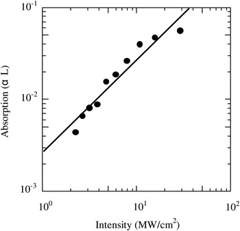
Figure 42 shows two photon absorption of Rh:BaTiO₃ crystal as a function of the pump intensity measured by z-scan method. A pump laser used was a 1.55 µm femtosecond fiber laser (IMRA co.) with a pulse width of 100 fs and a pulse repetition frequency of 50 MHz. Two-photon absorption was evidenced by that absorption of the crystal was almost proportional to pump intensity. And the absorption of the crystal reached up to the saturation level above the pump intensity of 30–40 MW/cm².

Fig. 42.

Two photon absorption as a function of pump intensity in Rh:BaTiO₃.

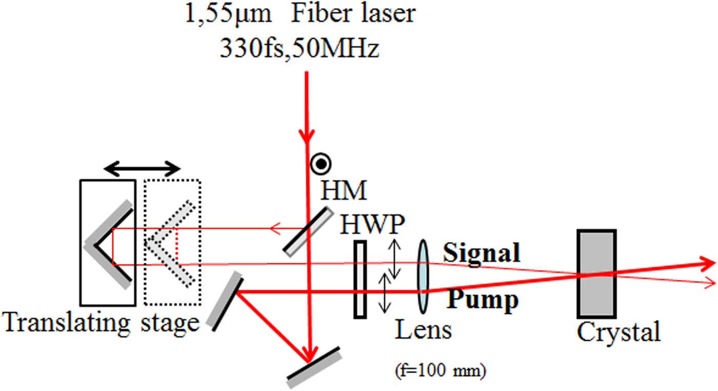
Two-wave mixing gain due to two-photon absorption was also measured. Figure 43 shows a schematic diagram of an experimental setup. The laser used was a 1.55 µm femtosecond fiber laser (IMRA co.) with a pulse width of 100 fs and a pulse repetition frequency of 50 MHz, and its output was split into a p-polarized probe and strong pump beams with an intensity ratio of 1:9. The two beams were focused to be a ϕ50 µm spot onto a thin 45^°-cut Rh:BaTiO₃ crystal (thickness 2 mm) and a Te doped SPS crystal, the angle between two beams was about 9^°. With this setup, the effective interaction length between the probe and pump beams was estimated to be about 0.3 mm. We also optimized an optical delay of the pump beam to the probe beam, thereby yielding good temporal overlap between probe and pump beams. The power of the two beams was controlled by an attenuator.

Fig. 43.

(Color online) Experimental setup.

Two-wave mixing gain exhibited the significant intensity dependence of the pump beam, and it reached up to about 4.5 cm⁻¹ at the maximum pump level. The two-wave mixing gain in our experiment was less than that obtained by the continuous-wave laser pumping, and it was impacted by relatively large spectral bandwidth of 10–15 nm associated with the femto-second pulses. The crystal showed a faster temporal response (<100 s) than the un-doped BaTiO₃ (200–300 s), resulting from that the Rh ions formed shallow traps and they improved two photon absorption efficiency (Fig. 44).

Fig. 44.

Two-wave mixing gain as a function of pump intensity in Rh:BaTiO₃ based on two photon absorption.

Two-wave mixing gain in Te doped Sn₂P₂S₆ was also measured by using the same setup. A maximum two-wave mixing gain of 1.68 cm⁻¹ was obtained at the pump intensity of 26 W/cm² (Fig. 45). To investigate contribution of two-photon absorption to photorefractive two-wave mixing, we also measured two-wave mixing gain based on one photon absorption by using the same setup. A 1.55 µm continuous-wave laser diode in combination with a fiber amplifier was used, and its output power was about 200 mW. The effective two-wave mixing gain was impacted by too short interaction (~0.3 mm) between the probe and pump beams even at the maximum pump level, and it was measured to be 0.92 cm⁻¹. They evidenced that the two-photon absorption improved significantly the photorefractive activity at 1.55 µm in the SPS crystal. We also measured 1.55 µm two-wave mixing gain based on one-photon absorption by optimizing experimental parameters including the beam size and the incident angle of probe and pump beams onto the SPS crystal. Figure 46 shows an experimental two-wave mixing gain as a function of the grating period formed by probe and pump beams. The pump beam intensity was then 28 W/cm², and a power ratio of the pump beam to the probe beam was 1:98. A maximum gain of 1.02 cm⁻¹ at a grating period of 1.53 µm was measured, and it was still less than that observed by 1.55 µm femto-second laser. For the Rh:BaTiO₃ crystal, we could not observe any two-wave mixing gain based on one photon absorption at all.

Fig. 45.

(Color online) Two wave mixing gain as a function of pump intensity in Te: Sn2P2S6 using 1.55 µm CW and femtosecond laser.

Fig. 46.

Two-wave mixing gain as a function of the grating spacing in 1% Te-doped Sn₂P₂S₆ for the wavelengths 1.55 µm.

7.1. Introduction

The formation of volume holographic grating in photo-refractive (PR) crystals can be used for the dispersion compensation (Roblin et al., Reference Roblin, Gires, Grousson and Lavallard1987), storing (Acioli et al., Reference Acioli, Ulman, Ippen, Fujimoto, Kong, Chen and Cronin-Golomb1991), shaping, and the amplification (Yao & Feinberg, Reference Yao and Feinberg1993) of ultrashort laser pulses. PR volume gratings are also applicable as a self-pumped phase-conjugate mirror for short laser pulses (Jain & Stenersen, Reference Jain and Stenersen1984). Yau et al. (Reference Yau, Wang, Pan, Chen and Chang1997) reported self-pumped phase conjugation (SPPC) in BaTiO3 with picosecond and femtosecond laser pulses at 800 nm. Joubert et al. (Reference Joubert, Roblin and Grousson1989) first studied the temporal reversal of picosecond optical pulses by phase conjugation in Fe:LN.

In these early studies, the role of chirped volume grating for recording and amplifying broadband optical laser pulses was not explored. Nishioka et al. (2007) recently proposed that the chirped volume grating formed in a Fe:LN crystal can be utilized to amplify a few cycle femtosecond laser pulses. The PR effects in wide band gap (4 eV) LN (Beyer et al., Reference Beyer, Breunig, Kalkum and Buse2006) crystal with femtosecond laser pulses in the near-infrared regime can be governed by either linear one-photon or nonlinear two-photon absorption (TPA) using iron impurity centers, depending on the crystal doping concentration, and the intensity of the writing laser pulses. Although the proposal of femtosecond laser pulse amplification by chirped volume grating written in an Fe:LN crystal at 800 nm by Nishioka et al. (2007) was based on two-photon absorption and their experimental results were also interpreted with TPA, no research report shows direct evidence of TPA at 800 nm in Fe:LN crystals.

In this work, we demonstrate photorefractive two-wave mixing amplification of femtosecond laser pulses generated from a Ti:Al₂O₃ regenerative amplifier at 1 kHz in an Fe:LN crystal and confirm that one-photon absorption remains dominant in the Fe:LN crystal up to 100 GW/cm². A potential possibility of two-step holographic recording in a Fe:LN crystal using ultrashort laser pulses is also experimentally investigated.

7.2. Absorption of Fe:LN at 800 nm

The measurement of light absorption was performed using a balanced detection technique. The laser source was a mode-locked Ti:Al₂O₃ oscillator that generates 30-fs (full width at half maximum (full width at half maximum = FWHM)) femtosecond laser pulses at 800 nm and a repetition rate of 76 MHz. The spatial spot diameter (at 1/e² intensity level) of the laser beam was about 2 mm. Absorption was measured up to about 5 GW/cm² for 76-MHz oscillator pulses. A 2-mm-thick Fe:LN (Fe concentration: 0.05 mol%) crystal was used to measure the light-absorption coefficient. The c-axis of the crystal was kept parallel to the light polarization. We also measured the light absorption of the same Fe:LN crystal using laser pulses amplified by the regenerative amplifier at 1 kHz at an incident laser intensity ranging from 10 to 388 GW/cm².

Figure 47 shows the experimental results of the absorbed laser power for ordinarily polarized light. The absorption power almost linearly increases as the incident laser power increases up to about 100 GW/cm². The corresponding linear absorption coefficient is about 0.11 cm. On the other hand, an abrupt increase in the absorption coefficient was observed above 100 GW/cm². This highly nonlinear absorption starting at about 100 GW/cm² could be a multi-photon process associated with second-harmonics light (Von der Linde et al., Reference Von Der Linde, Glass and Rodgers1974). In fact, we observed substantial 400-nm second-harmonic emission from the crystal. Significantly, the crystal failed to exhibit any damage even at 388 GW/cm². From the obtained results, the pulses are obviously not subject to nonlinear absorption up to nearly the 100-GW/cm² intensity, and the PR effects induced in the Fe:LN crystal with illumination of the femtosecond laser pulses at 800-nm wavelength reflects one-photon absorption by the impurity iron centers. It has also been reported (Pettazzi et al., Reference Pettazzi, Alonzo, Centini, Petris, Vlad, Chauvet and Fazio2007) that the refractive-index changes in pure LN crystal by TPA are negligible for 800-nm femtosecond laser pulses below 100 GW/cm², although even pure LN contains a low but significant amount of iron impurity at concentrations of 0.001 to 0.01 wt% (Clark et al., Reference Clark, Disalvo, Glass and Peterson1973).

Fig. 47.

(Color online) Absorption of 800-nm femtosecond laser pulses at peak intensity ranging from 15 MW/cm² to 388 GW/cm² in an Fe:LN.

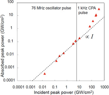
7.3. Grating Formation with Chirped Laser Pulses

PR volume phase gratings were formed in the same crystal that was used to measure the absorption coefficient. Figure 48 shows the experimental setup for grating formation by low-energy 76-MHz pulses at 800 nm. 30 fs (FWHM) pulses were generated from a mode-locked Ti:Al₂O₃ laser oscillator with output energy of 5 nJ/pulse. The laser beam was split into two beams: a pump beam (I _p) and a signal beam (I _s) by a beam splitter (BS). A 40-mm-thick fused silica block was used to stretch the temporal width of the signal pulse to 210 fs. The writing half-angle of the incident beams was fixed in such a way that grating spacing of 5.22 µm was formed in the crystal. The pump and signal beams entered the crystal symmetrically in a plane containing the crystal's c-axis so that the grating vector became parallel to the c-axis of the crystal. The polarization of the writing beams was also made parallel to the crystal's c-axis. The spatial spot diameter (at 1/e² intensity level) of the two beams was 2 mm. A 100-cm focal length lens was used to adjust the beam diameter onto the front face of the crystal.

Fig. 48.

Experimental setup for monitoring grating formation in TWM experiment. BS = Beam Splitter, M = Mirror, NDF = Neutral density filter, PD = Photo-detector, and L = Lens.

We performed grating generation using strong amplified laser pulses at 800 nm intensity level of the two beams was 2 mm. A 100-cm focal length lens was used to adjust the beam diameter onto the front face of the crystal. We performed grating generation using strong amplified laser pulses at 800 nm, produced by the regenerative chirp pulse amplifier (CPA). The output energy of the amplified laser pulses at a repetition rate of 1 kHz was 0.4 mJ/pulse after the pulse compression. The shortest pulse width (FWHM) of the output pulses after the compression was about 50 fs. The experimental setup including a pulse shaper was almost the same as that with the oscillator laser pulses (Fig. 48). The pump pulse width stretched by the 40-mm-thick fused silica block was 166 fs.

The experimental results for the evolution of the diffraction intensity from the PR grating written by laser pulses generated from the amplifier are shown in Figure 49. The summary is listed in Table 2. The diffracted signal from the recorded gratings written by unstretched pulses is extremely low. For the unfocused beam recording condition (2-mm beam diameter), a maximum diffraction efficiency of 0.8% was obtained for writing pulse peak intensities of I _p = 2.63 MW/cm² and I _s = 0.11 MW/cm². Here, we defined the diffraction efficiency as the fraction of the average power of the diffracted pump beam relative to the incident pump beam power. On the other hand, for a stretched signal pulse at I _s = 0.012 MW/cm² and an unstretched pump pulse at I _p = 2.63 MW/cm², a maximum diffraction efficiency of 4.8% was obtained after 1800 s. For the focused beam recording condition (0.46-mm beam diameter), when the signal pulses were not stretched (I _p = 58.3 MW/cm², I _s = 2.44 MW/cm²), we observed extremely weak diffracted signal at a diffraction efficiency of about 0.8%. However, when the signal pulse was stretched (I _p = 58.3 MW/cm², I _s = 0.27 MW/cm²) a maximum diffraction efficiency of 13% was obtained after 600 s.

Fig. 49.

(Color online) Temporal evolution of diffracted signals of pump beam of 800-nm cw and femtosecond pulse lasers generated from a mode-locked Ti:Al₂O₃ laser and a regenerative chirped pulse amplifier (CPA) in TWM experiments. Experimental conditions and highest diffraction efficiencies were summarized for each plot symbol in Table 2.

Table 2.

Sum mary of diffractive volume grating formation. Lines 1–6 correspond to plots in Figure 3

Note that when we formed the PR grating with continuous wave (cw) laser beams at 800-nm wavelength, the diffraction efficiency was always higher than that of the pulse recording for both the unfocused and focused beam recording conditions for a particular recording time for the same average recording powers at (I _s = 2.5 W/cm² and I _p = 5.5 W/cm²) and (I _s = 59 W/cm² and I _p = 126 W/cm²) (Fig. 49). This higher diffraction efficiency attributes to better visibility of the photo induced gratings and perfect phase matching on the diffraction caused by monochromatic light.

With the amplified laser pulses operating at 1 kHz, we obtained maximum diffraction efficiency of 17% after 780 s when we applied peak pulse intensities I _p = 15 GW/cm² and I _s = 31 GW/cm² to the pump pulse (166 fs), and the signal pulse (50 fs), respectively. The main obstacle in generating high diffraction efficiency from the grating formed by the femtosecond laser pulses is its extremely short coherence length. Because of this extremely short coherence length (short pulse duration), the grating width formed by two interfering pulses is much smaller than that of the beam overlapping width. Therefore when two Fourier transform limit femtosecond pulses overlap in the crystal, they can only form a few high contrast interference fringes in the central region of the overlapping beams, whose width is on the order of micrometer and only the central portion of the interacting beams can diffract from this thin grating, resulting in low diffraction efficiency. On the other hand, when we stretch one of the writing pulses, because of its longer duration, the grating width increases, as a result, a relatively large portion of the interacting beams diffracts from this wider grating and produces relatively high diffraction efficiency. However, the possibility of degradation exists in the phase matching of different frequency components when they diffract from the gratings formed by frequency components other than their own, even in chirped volume grating.

A two-wave mixing amplification experiment was also carried out with high-energy laser pulses operated at 1 kHz. The average power ratio of the signal to pump beam was kept to 1:17.4. The average power of the pump pulsed beam was 260 mW, and the pump pulse was stretched from 50 to 480 fs by a fused silica glass block. The average power of the signal beam was 15 mW. The amplification of the weak signal pulse by 34% was measured. By applying a proper amount of frequency chirp to the pump pulse and setting small grating spacing, higher amplification might be achieved. The amplified signal pulse shifted slightly toward the high-frequency components due to the phase-mismatched diffraction of different frequency components from the secondary gratings caused by the two wave mixing (TWM) of the different frequency components of the interacting beams.

7.4. Two-Step Holographic Recording

The most effective approach to record near infrared (NIR) or infrared (IR) femtosecond laser pulses within short times is a two-step recording technique using short-wavelength gating laser pulses. The principle of gated recording can be understood by a two-center charge transport model (Jermann et al., Reference Jermann, Simon and Krätzig1995) (Fig. 50). Iron dopants lead to Fe²⁺-centers that are “deep” levels, whereas the second Nb⁺⁵_Li center is more “shallow.” Electrons can be excited from Fe²⁺ by short-wavelength gating pulses, forming Fe³⁺. Electrons are excited either to the conduction band or to the shallow traps, resulting in the formation of the Nb⁺⁴_Li state. NIR/IR laser pulses have insufficient energy for the excitation of electrons from the deeper Fe²⁺ sites to the conduction band. By illuminating the crystal with short-wavelength gating (blue or green) light G, shallow traps are filled, and the crystal will therefore be sensitized for subsequent holographic recording with NIR/IR light from the Nb⁺⁴_Li centers.

Fig. 50.

Band diagram for two-center charge transport model in Fe:LN. The arrows indicate the excitation and recombination of electrons.

To verify the two-step recording scheme, we employed 1.06-μm recording laser pulses and 532-nm (SHG) gating pulses to form a volume hologram. The incident laser energy of the 1.06-μm recording pulses was 7.8 mJ/pulse and the laser pulse width was 15 ns, whereas the incident laser energy of the 532-nm gating pulse was varied at 0.3, 1, and 7 mJ/pulses. The pulse repetition rate was 20 Hz. Without the gating pulse no diffraction was observed by a HeNe reading laser. Figure 51 shows the temporal evolution of the gratings at various gating laser energies. The summary is listed in Table 3.

Fig. 51.

Temporal evolution of volume holographic gratings in a scheme of two-step writing with 1.06-μm recording pulse and 532-nm gating pulse at incident energy of (a) 7 mJ, (b) 1 mJ, and (c) 0.3 mJ.

Table 3.

Summary of two-step holographic recording using ns-laser pulses

During the two-step recording experiment with femtosecond lasers, second harmonic generation femtosecond laser pulses uniformly irradiate the crystal at the same repetition rate as the 800-nm laser pulses. Since the gating pulses also act as an erasing pulse, the incident laser fluence and the delay time must be adjusted to obtain the highest diffraction efficiency.

We formed gratings in the same crystal by two-step excitation process using the recording setup that resembles the one in Figure 48. The recording pulse peak intensities and pulse widths for the pump and signal beams were identical as those used in the one-step excitation recording process. A 400-nm femtosecond laser pulse (230 fs) of peak intensity 84 MW/cm² was simultaneously allowed to sensitize the crystal during grating formation. A maximum diffraction efficiency of 9% was obtained after 540 s. The grating formation speed in the two-step excitation process is relatively faster than that of the one-step excitation process with high-energy CPA pulses, even in this case where second harmonic light was also generated. Therefore, the two-step excitation process can be an alternative recording scheme to efficiently form grating in Fe:LN crystal by high-energy and low repetition 800-m femtosecond laser pulses at 1 kHz.

ACKNOWLEDGMENTS

This research was supported by a Grant-in-aid from the Ministry of Education, Culture, Sports, Science, and Technology, Japan for the Photon Frontier Network Program.

Abstract

A highly stable, ultrahigh repetition rate train of user-specified, complex ultrashort pulses is synthesized by precise manipulation of spectral phases of adiabatically generated rotational Raman sidebands using a specially designed spatial phase controller and spectral interferometer.

9.1. Introduction

Recently, user-specified, complex waveform synthesis has gained significance in applications related quantum control, and optical communications (Levis et al., Reference Levis, Menkir and Rabitz2001; Jiang et al., Reference Jiang, Huang, Leaird and Weiner2007). Numerous attempts have been reported to generate such waveforms using Raman sidebands (Shverdin et al., Reference Shverdin, Walker, Yavuz, Yin and Harris2005; Katsuragawa et al., Reference Katsuragawa, Yokoyama, Onose and Misawa2005; Chen et al., Reference Chen, Hsieh, Huang, Su, Lai, Tang, Lin, Lee, Pan, Pan and Kung2008). This work proposes a new method based on the combination of a suitable line-by-line phase controller with adiabatically generated discrete Raman sidebands for an efficient generation of arbitrary optical waveforms (AOWs). The advantage in this work over previous studies is adaptive, accurate measurement of the discrete spectral phase, and the line-by-line manipulation of spectral phases using a high damage threshold phase controller. The generated AOWs can be applicable to study pulse-shape dependence stimulated Brillouin scattering (Brent et al., Reference Brent, Neuman and Hackel1992) and selective enhancement of optical phonons (Hase, Reference Hase, Itano, Mizoguchi and Nakashima1998).

9.2. Experimental Details

The experimental schematic is shown in Figure 53. The two pump laser radiations, Ω₀: 382.4280 THz (783.9186 nm) and Ω₋₁: 371.8050 THz (806.3162 nm) are produced with a dual-frequency injection-locked nanosecond pulsed Ti:Sapphire laser (Katsuragawa & Onose, Reference Katsuragawa and Onose2005), which provide Fourier-transform limited 6-ns pulses (spectral width about 50 MHz) and completely overlap each other temporally and spatially. The differential frequency is slightly detuned by 990 MHz from the Raman resonance (J = 2 ← 0 transition of parahydrogen) to satisfy the adiabatic condition. The two pump laser beams are then loosely focused in the parahydrogen chamber (temperature: 77 K, density: 3 × 10²⁰ cm⁻³) with f = 800 mm lens to a peak intensity 4.5 GW/cm². Raman sidebands are generated in the forward direction (Sokolov et al., Reference Sokolov, Walker, Yavuz, Yin and Harris2000; Liang et al., Reference Liang, Katsuragawa, Kien and Hakuta2000; Suzuki et al., Reference Suzuki, Hirai and Katsuragawa2008a) and then introduced into the spectral line-by-line phase controller (SLLPC) after being collimated with a f = 300 mm lens. The SLLPC is a spatial phase modulator consisting of 48 fused-silica plates and configured in a folded 4f-configuration (Suda et al., Reference Suda, Oishi, Nagasaka, Wang and Midorikawa2001). The incident Raman sidebands are dispersed with a grating (600 grooves per mm) and each sideband is focused onto a single glass plate placed in the Fourier plane with the use of a concave mirror (f = 0.5 m). The change in the spectral phase of each sideband is accomplished by changing the angle of the corresponding fused-silica plate through a Piezo actuator (minimum resolution: ±0.1 rad, which was limited by the minimum step voltage (1 V) applied to the Piezo in the spectral line-by-line phase controller system). The phase controlled Raman sidebands and the corresponding waveform in the time domain are characterized by using modified spectral-phase interferometry for a direct electric-field reconstruction system for discrete spectra (SPIDER-DS) (Suzuki, Reference Suzuki, Sawayama and Katsuragawa2008b). The SPIDER-DS system operates rapidly and generates an error signal, which is fed back to the SLLPC system through a set of 48-channel digital-to-analog converters and amplifiers (Kanaka et al., Reference Kanaka, Raju, Suzuki, Suda, Midorikawa and Katsuragawa2010).

Fig. 53.

(Color online) (a) Photographic image of Raman sidebands, (b) Raman sidebands spectrum from Ω₋₅ to Ω₆. Seven sidebands (Ω₋₄: 339.936 THz to Ω₂: 403.674 THz) are chosen for line-by-line phase control to the target as highlighted by box.

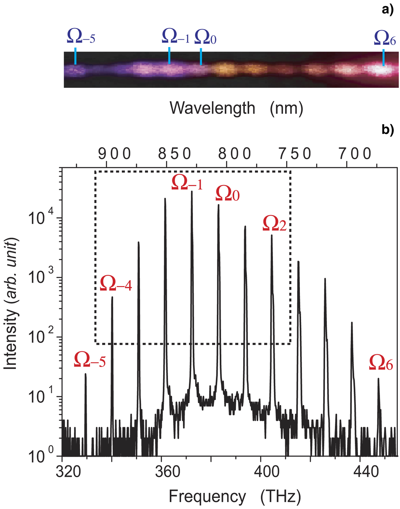
9.3. Results and Discussions

The photographic image of generated Raman sideband and its spectrum are shown in Figure 54a and 54b, respectively. Twelve Raman sidebands, from Ω₋₅: 329.3070 THz (910.3738 nm) to Ω₆: 446.1578 THz (671.9426 nm), are observed. The generated sidebands are collimated and guided to the SLLPC system. Among these sidebands, seven are chosen from Ω₋₄ to Ω₂ by partly blocking the others in space in the SLLPC (highlighted by box in Fig. 53b). This selection is done to restrict the Raman sidebands to those that could produce sufficient SPIDER-DS signals.

Fig. 54.

(Color online) Reconstructed temporal intensity waveforms on the basis of the estimated spectral phases of the Raman sidebands. Crimson line is the waveform at the end of optimization process. Black line shows the Fourier-transform-limited waveform.

In this work, we precisely control the relative spectral phases of the Raman sidebands to a target “flat-relative spectral phase.” This target implies Fourier-transform limited ultrashort pulse train with a pulse duration corresponding to the inverse of the frequency spacing of the Raman sidebands in the time domain. We reconstructed the intensity waveforms consisting of seven Raman sidebands in the time domain using spectral phase of Raman sidebands measured with SPIDER-DS and intensity of Raman sidebands. We can see that as a result of controlling the relative spectral phase to the target, a train of 17 fs ultrashort pulses (crimson line in Fig. 55) is formed with a 94-fs time interval (10.6-THz repetition rate), which precisely corresponds to the inverse of the frequency spacing of the Raman sidebands. The pulse shape is in good agreement with the target Fourier-transform-limited ultrashort pulse (black line in Fig. 55).

Fig. 55.

(Color online) Generation of an ultrahigh repetition rate train of rectangular waveforms. (a) Spectral phases (Black dotted line = effective target, red line = achieved phase) and power spectrum (in gray) of the Raman sidebands. (b) A train of rectangular pulses = ideal waveform (blue line), effective target waveform (black line), and the achieved waveform (red line).

We demonstrated AOW generation by line-by-line control on Raman sidebands. An example is shown for rectangular optical waveform generation. We performed numerical simulations to obtain effective target spectral phase and waveform (black line in Figs. 56a and 56b, respectively) using seven Raman sidebands in comparison with ideal target waveform (black line in Fig. 55b). To ensure that the spectral phases converge sufficiently with the effective target in the experiment, we followed an iterative phase manipulation process based on the precise phase measurement provided by the SPIDER-DS (error signal is produced from the SPIDER-DS measurement). The achieved spectral phase and waveform after iterative process is shown by red line in Figures 55a and 55b, respectively. A precise match with the effective target is found in both spectral phase and waveform shape except for small deviations due to the precision of the phase control (about ±0.1 rad).

Fig. 56.

Theoretical simulation of the dependence of the output energy on G. Line AB represents a linear increase of output energy below the SBS threshold. Line CD shows the optical limiting above the SBS threshold. Dashed lines, linear fit of lines AB and CD. The vertical dashed-dotted lines represent intersection points that correspond to the SBS threshold.

10.1. Introduction

Stimulated Brillouin scattering (SBS) has received general attention owing to its broad applications such as beam combination (Kong et al., Reference Kong, Yoon, Shin and Beak2008, Reference Kong, Shin, Yoon and Beak2009a; Wang et al., Reference Wang, Lu, He, Zheng and Zhao2009a, Reference Wang, Lu, Wang, Zheng, He and Lin2009b; Ostermeyer et al., Reference Ostermeyer, Kong, Kovalev, Harrison, Fotiadi, Megret, Kalal, Slezak, Yoon, Shin, Beak, Lee, Lu, Wang, Lin, Knight, Kotova, Straber, Scheikhobeid, Riesbeck, Meister, Eichler, Wang, He, Yoshida, Fujita, Nakatsuka, Hatae, Park, Lim, Omatsu, Nawata, Shiba, Antipov, Kuznetsov and Zakharov2008), Brillouin amplification of weak signals (Gao et al., Reference Gao, Lu, He, Dong and Hasi2009; Lu et al., Reference Lu, Gao, He, Zhang and Hasi2009), optical limiting for laser protection in high-power laser (Hasi et al., Reference Hasi, Lu, Fu, Lu, Gong, Lin and He2009b, Reference Hasi, Guo, Lu, Fu, Gong, Geng, Lu, Lin and He2009c), and slow light in optical fiber (Kovalev et al., Reference Kovalev, Kotova and Harrison2009; Lu et al., Reference Lu, Dong and Li2007). Among the parameters that characterize SBS, the threshold value is of great importance. The definition of this parameter was first suggested to be pump intensity when the SBS amplification of the Stokes radiation overcomes its losses in a medium (Chiao et al., Reference Chiao, Townes and Stoicheff1964). However, the amplification of the Stokes signal corresponding to the point of transition is too weak to detect for most SBS media because of the lower losses. Thus, the threshold is usually considered as the pump intensity when the SBS reflectivity reaches 1%, 2%, or 5% (Boyd et al., Reference Boyd, Rzazewski and Narum1990; Eichler et al., Reference Eichler, Konig, Piitzold and Schwartz1995). As we know, this is a rather confusing experimental practice. Recently, Bai et al. (Reference Bai, Shi, Ouyang, Chen, Gong, Jing, Liu and Liu2008) presented a method to determine the threshold value of SBS by the point of the deviation of the value of the attenuation coefficients of wide- and narrow-line width lasers. We find it is feasible for some media (e.g., CS₂, water, etc.), but it is not for other media (e.g., FC-75, FC-72, etc.). Because the SBS still occurs in these media such as FC-75 and FC-72 when the wide-line width laser is used (Lee et al., Reference Lee, Lee and Kong2005b), the attenuation coefficients of the media will not be constants. Thus, the point of the deviation can not be determined.

Usually, it is more appropriate and convenient to characterize the steady-state or transient SBS by its threshold exponential gain, G _th = gI _thL _eff, where g is the SBS gain coefficient of the medium, I _th is the SBS threshold pump intensity, L _eff is the effective interaction length (Kovalev & Harrison, Reference Kovalev and Harrison2007; Bel'dyugin et al., Reference Bel'dyugin, Efimkov, Mikhailov and Zubarev2005). Moreover, the value of G _th can provide a practically important reference for the design of a Brillouin amplifier, since the optimum working point of the amplifier is usually near to G _th (Sternklar et al., Reference Sternklar, Glick and Jackel1992). When the steady-state approximation is considered and 1% (SBS reflectivity) criterion for threshold is used, Boyd et al. (Reference Boyd, Rzazewski and Narum1990) predicted that the value of G _th in organic liquids is in the range 20–25, and Kovalev and Harrison (Reference Kovalev and Harrison2007) found that the value of G _th decreases with increasing the interaction length in optical fiber. When a laser system with the nanosecond-order pulse width is used, for the most media (the phonon lifetime is usually between 0.1 ns and 10 ns (Erokhin et al., Reference Erokhin, Kovalev and FaïZullov1986; Yoshida et al., Reference Yoshida, Kmetik, Fujita, Nakatsuka, T. Yamanaka and Yoshida1997)), the transient theory should be use to analyze the SBS process (Bel'dyugin et al., Reference Bel'dyugin, Efimkov, Mikhailov and Zubarev2005). Nevertheless, to our knowledge, the dependence of G _th on the pump wavelength and the interaction length in the transient regime has not been observed experimentally or treated theoretically.

In this work, we present a new method to measure the SBS threshold, which is simple, accurate, and is not confined by the medium characteristics. By this method, we theoretically and experimentally investigate the dependences of the values of G _th on the pump wavelength and the interaction length.

10.2. Measurement Principle and Threshold Characteristics for SBS

We assume a pump wave , propagating in the +z direction, a backward Stokes wave, , and a forward acoustic wave, , within the SBS medium. The three-wave coupled wave equations to describe transient SBS including its spontaneous initiation from noise are written as (Gaeta & Boyd, Reference Gaeta and Boyd1991)

(1a)

(1b)

(1c)

where E _P, E _S, and ρ are the amplitudes of the pump, the Stokes, and the acoustic waves, respectively; n is the refractive index of the medium; g ₁ and g ₂ are the coupling coefficients; α is the absorption coefficient; Γ = 1/τ₀ denotes the phonon decay rate, where τ₀ is the phonon lifetime. Also, f represents the Langevin noise source that describes the thermal excitation of acoustic waves and leads to the initiation of the SBS process. It is spatially and temporally δ-correlated Gaussian random process with zero mean:

(2)

where

(3)

characterizes the noise intensity. ρ and V are the density and sound speed of the medium, respectively; A is the cross-sectional area of the interaction region. Directly, integrating the ρ phonon from Eq. (1c), substituting it into Eqs. (1a) and (1b), and using the transforms g = 4g ₁g ₂/Γ·8π/nc, and we have

(4a)

(4b)

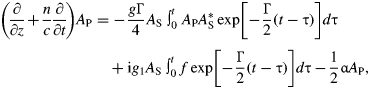
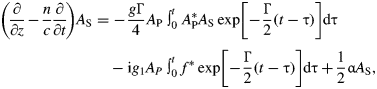
where g is the SBS gain coefficient. The beam intensity is defined as I _P,S = | A _P,S| ². By implicit finite difference in time and backward difference in space, Eq. (4) can be numerically solved.

We consider an incident pump pulse of Gaussian temporal shape, which is input at z = 0, and output at z = L (L is the cell length). The boundary conditions are given as: A _P(0, t) = A _P0 exp {− 2 ln 2[(t − t ₀)/t _P]²}, A _S(L, t) = 0. The pump output energy can be expressed as ʃ₀^∞ |A _P(L, t)|²dt. The system's exponential gain is defined as G = gI _P0L _eff, where I _P0 =|A _P0| ² is the peak intensity of the incident pump pulse. Obviously, for given g and L _eff, the value of G is changed with I _P0. Figure 57 shows that the dependence of the output energy of the pump on the exponential gain G. In the calculation, the following parameters are used: the wavelength of the incident pump pulse is 532 nm with an 8 ns full width at half maximum, the interaction length is 60 cm. FC-72 is chosen as the SBS medium, its parameters are shown in Table 6. The simulation parameters are closely matched to those that are used for experiments.

Fig. 57.

Dependences of G _th in CS₂ and FC-72 on (a) λ for L _eff = 60 cm, (b) L _eff for λ = 532 nm.

Table 6.

The parameters of some SBS media

^aThe parameters are calculated according to the equation given by Erokhin et al. (1986) and the results at 1064 nm (Erokhin et al., 1986; Yoshida et al., 1997); Others are quoted from Erokhin et al. (1986) and Yoshida et al. (1997).

We see that when the value of G is low, the SBS does not take place, and hence the line AB in Figure 56 shows a linear increase of output energy with G. After the pump intensity exceeds the SBS threshold, the energy quickly transfers from the pump to the Stokes. Consequently, the increase rate of output energy slows down (i.e., line CD), leading to an optical limiting effect. Line CD represents a nonlinear increase process. However, according to Figure 56, it can be considered as an approximately linear change before the gain saturation occurs. Thus, we perform linear fits for lines AB and CD. The value of G corresponding to the intersection point of two straight lines is defined as G _th. At this time, the SBS reflectivity is about 2.5%, which agrees with the criterion for threshold generally accepted.

By using the model and method mentioned above, we obtain the values of G _th for different wavelengths, λ, and interaction lengths, L _eff, using CS₂ and FC-72 as the SBS media. Their main medium parameters are listed in Table 6. Figure 58a shows the dependence of G _th on λ. According to the literature (Damzen, et al., Reference Damzen, Hutchinson and Schroeder1987), the phonon lifetime of the medium, τ₀, is proportional to λ². Therefore, with the increase of λ, the ratio of the pump pulse width to the phonon lifetime, t _P/τ ₀, decreases, leading to the stronger transient behavior (Bel'dyugin et al., Reference Bel'dyugin, Efimkov, Mikhailov and Zubarev2005; Maier & Renner, Reference Maier and Renner1971). This causes the increase of the values of I _th and G _th. On the other hand, we can see from Eq. (3) that the noise intensity, Q, is proportional to Γ, i.e., Q ∝1/τ₀·G _th will be raised because of the reduced Q with increasing λ. Then, we choose λ as 532 nm and study the dependence of G _th on L _eff, as shown is in Figure 58b. At this time, t _P/τ₀ is 5 and 27 for CS₂ and FC-72, respectively. Strictly speaking, the transient SBS process will occur in these two media (Bel'dyugin et al., Reference Bel'dyugin, Efimkov, Mikhailov and Zubarev2005). In the transient regime, the longer L _eff for the same G means the smaller pump intensity, which results in a slower build up of the sound wave and hence a smaller Stokes signal intensity. Therefore, the larger G _th is needed to attain the SBS threshold. It can also be seen from Figure 58 that the values of G _th are very different for various media, and are larger than that of steady state (20–25 (Boyd et al., Reference Boyd, Rzazewski and Narum1990)). This also indicates that G _th increases as t _P/τ₀ decreases due to the transient effect.

Fig. 58.

Output energy versus G in (a) CS₂ at λ = 532 nm, (b) FC-72 at λ = 532 nm, (c) CS₂ at λ = 1064 nm, and (d) FC-72 at l.1064 nm.

10.3. Experimental Results and Discussions

Experimental setup is shown in Figure 59. The laser used is an injection-seeded, Q-switched, pulsed Nd:YAG laser (Continuum Powerlite Precision II 9010) with a line width of 90 MHz and repetition rate of 10 Hz. The output wavelength of the laser is 1064 nm and 532 nm (when the double frequency crystal is inserted), the pulse width is 7–8 ns, and the beam diameter is 8 mm. The pump energy is continuously varied by means of an attenuator, which consisted of a rotatable half-wave plate (λ/2) and a polarizer (P). A quarter-wave plate (λ/4), together with the polarizer P, forms a light isolator, preventing backward SBS light from entering YAG oscillator. A small fraction of the laser energy separated by the beam splitter (BS) and the output energy of the pump is measured by the PE50BB energy detectors (Ophir Optics), ED₁ and ED₂, respectively.

Fig. 59.

G_th versus L.

CS₂ and FC-72 are chosen as SBS media. It has been theoretically and experimentally validated that the scattering occurred in these media could only be SBS if the pulse energy of the laser is controlled in certain range. Other stimulated scatterings can be excluded (Bai et al., Reference Bai, Shi, Ouyang, Chen, Gong, Jing, Liu and Liu2008; Gao et al., Reference Gao, Lu, He, Hasi and Zhang2008; Daree & Kaiser, Reference Daree and Kaiser1971; Sen & Sen, Reference Sen and Sen1986). SBS generally takes place in the free gain length (FGL) determined by the pulse width of the pump beam (Bai et al., Reference Bai, Shi, Ouyang, Chen, Gong, Jing, Liu and Liu2008). In our experiments, the FGLs in CS₂ and FC-72 are about 75 cm and 95 cm, respectively. If the cell length, L ≥ FGL, L _eff = FGL, or else, L _eff = L. Figure 60 shows that the output energy versus G at 532 nm and 1064 nm. The cell lengths are all 60 cm, which are all less than the FGLs. Therefore, L _eff = 60 cm. To determine G _th, the measured results below and above the SBS threshold are fitted into two straight dash lines. The vertical dash-dot lines denote intersection points that correspond to G _th. The measured and theoretical G _th and I _th are summarized in Table 7. It can be seen that the values of G _th and I _th increase as λ. The reasons for this trend are discussed in the theoretical analysis.

Fig. 60.

(Color online) Model of non-collinear Brillouin amplification.

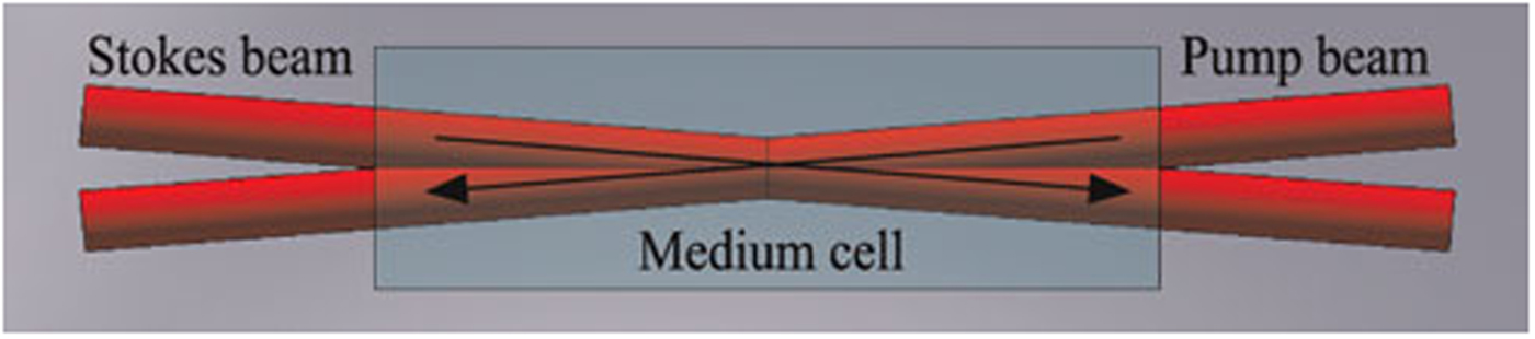
Figure 59 shows the dependence of G _th in CS₂ and FC-72 on the cell length, L. In the experiment, L are all less than FGLs, so L _eff = L. The pump wavelength is 532 nm. It can be seen that G _th increases as L. This result is different from that for steady-state SBS (Kovale & Harrison, 2007). The change tendencies of the experimental results are in agreement with those of the theoretical predictions in Figure 58b.

However, as seen from Table 7, there are the discrepancies between the experimental and theoretical values. The reasons for the errors may be summarized as follows. First, some main medium parameters such as g and τ₀ in the calculation are not completely consistent with those in the experiment, especially for the case of λ = 532 nm. Most of data in Table 6 quoted from the literatures are experimentally obtained at 1064 nm; whereas the parameters at 532 nm are calculated according to the equation given by Erokhin et al. (Reference Erokhin, Kovalev and FaïZullov1986) and the results at 1064 nm. Therefore, the relative measurement errors at 532 nm (about 8%) are larger than those at 1064 nm (<5%). Second, we find that the absorption coefficient has greater influence on the calculated results. In the theoretical calculation, we introduce the linear absorption coefficients without considering the nonlinear absorption that may occur in the media. Finally, one-dimensional coupled wave equations as shown in Eq. (1) approximately describe the SBS characteristics. If more accurate, Gaussian spatial and spectral distribution of the pump beam should be taken into account.

Table 7.

Comparison of measured and theoretical threshold exponential gain G_th and the threshold value I_th for SBS

ACKNOWLEDGMENTS

This work is supported by the National Natural Science Foundation of China (Grant No. 60878005, 60778019) and the Program of Excellent Team in Harbin Institute of Technology.

11.1. Introduction

Solid state lasers of high repetition rate, high power, and large energy may be widely applied in the domains of military, scientific research, and industry, such as inertial confinement fusion (Hoffmann et al., Reference Hoffmann, Blazevic, Ni, Rosmej, Roth, Tahir, Tauschwitz, Udrea, Varentsov, Weyrich and Maron2005; Miley et al., Reference Miley, Hora, Osman, Evans and Toups2005), space optical communication and material processing (Thareja & Sharma, Reference Thareja and Sharma2006; Veiko et al., Reference Veiko, Shakhno, Smirnov, Miaskovski and Nikishin2006). However, because of the limitation of crystal growth technology, heat distortion, and damage threshold, the output of a single-laser apparatus is restricted.

The laser beam combination is a technology that combines several laser beams with low power and energy to produce a high energy and high power laser output (Kong et al., Reference Kong, Lee and Lee2005c). Existing methods usually use a nonlinear optics phase conjugation approach to combine solid-state pulse lasers. Stimulated Brillouin scattering (SBS) is a very important way in these methods (Kong et al., Reference Kong, Lee, Shin, Byun, Park and Kim1997; Shuangyi et al., Reference Shuangyi, Zhiwei, Dianyang, Lei and Dongbin2007). The SBS parallel beam combination is composed of the overlap coupling beam combination (Basov et al., Reference Basov, Zubarev, Mironov, Mikhailov and Okulov1980), the back-seeding beam combination (Loree et al., Reference Loree, Watkins, Johnson, Kurnit and Fisher1987), and the self-phase control beam combination (Kong et al., Reference Kong, Lee and Lee2005b; Lee et al., Reference Lee, Lee and Kong2005b). The overlap coupling beam combination and the back-seeding beam combination are limited by the low load of the system and the poor backward reflectivity because several laser pulses are focused into one medium cell. In order to overcome these disadvantages, Kong et al. (Reference Kong, Lee and Lee2005b) proposed the self-phase control SBS parallel beam combination. In this new scheme, each laser pulse has an independent medium cell to realize phase conjugation, so that the system load is separated into many cells and is a simple optical arrangement (Kong et al., Reference Kong, Yoon, Shin and Beak2008). Their study indicated that the piston error between pump beams was the key factor of the beam combination (Kong et al., Reference Kong, Yoon, Beak, Shin, Lee and Lee2007b).

The serial laser beam combination based on Brillouin amplification uses several pump beams to amplify one seed pulse so that the phase is matched during the amplifying process. In this beam combination technology, the pump pulses and the seed pulse must be collinear to achieve the highest Brillouin amplifying efficiency. However, with increasing the number of pump beams, the beam combination structure becomes more and more complex because of a great amount of usage of polarizer and wave plates that are necessary to beam input and output in this system. Thus, in this work, we propose a non-collinear scheme to simplify the structure of the beam combination setup. Unlike the collinear scheme, there is an angle between the Stokes beam and the pump beam for the non-collinear scheme in the SBS cell. The pump pulse and the Stokes pulse can be injected into the amplification cell directly, and the amplified Stokes pulse is also output from the cell directly. So the polarizer and wave plates are not needed in the non-collinear scheme. Removing the wave plates and polarizer has significantly simplified the non-collinear scheme. With the non-collinear scheme, the key problem to be solved is achievement of high efficiency of the beam combination. In this article, the amplifying efficiency of the non-collinear scheme is investigated and discussed.

11.2. Theoretical Simulation

The geometry of non-collinear Brillouin amplification is shown in Figure 60, the angle between the Stokes beam and the pump beam is β. In this experiment, the pulse is a cylindrical beam so the intersection volume of the two beams is defined as the overlap volume V. The effective interaction length L _eff is defined by the result of V divided by the cross section area S. The beam diameter is given by d. So the effective interaction length L _eff in the medium cell is defined as

(1)

where

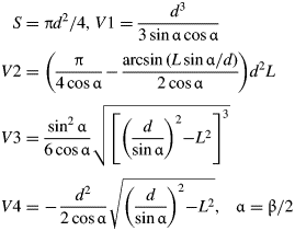
L is the length of the medium cell, and L _m is the length of the intersection domain. In the one-dimension transient condition, the non-collinear Brillouin amplification process is seen as a wave vector mismatch process. The wave vector direction is the pulse propagation direction. Thus, the mismatch angle is just the angle of the two beams. Finally, the numerical model of the non-collinear amplification is shown below (Shuangyi et al., Reference Shuangyi, Zhiwei, Dianyang, Lei and Dongbin2007).

(2a)

(2b)

(2c)

(2d)

Where g _max is the medium gain coefficient. E _P and E _S are the pump and Stokes fields, respectively.

Using this model, the non-collinear Brillouin amplification process is simulated. FC-72 is chosen as the SBS medium and its parameters are given by: gain coefficient g _max = 6.0 cm/GW, absorption coefficient α = 10⁻⁵cm⁻¹, medium refractive index n = 1.25, the Gaussian laser pulse widths are both 10 ns (full width at half maximum). As shown by Figure 60, the change of the angle will change the intersection area in the medium cell greatly, and therefore the effective interaction length changes too. Assuming that the cell length is 20 cm, the result according to Eq. (2) is shown in Figure 61. The angle impacts greatly on the effective interaction length. When the angle is nearly 90 mrad, the effective length reduces to half of the cell length. In other words, the cell length becomes short. But the change of the gain coefficient can be ignored. In conclusion, it is the effective interaction length that impacts the energy amplifying efficiency, but not the gain coefficient for this scheme. Fortunately, short cell length is good in the strong signal Brillouin amplification process. So the scheme is efficient in achieving high efficiency of amplification when the angle is limited within 200 mrad.

Fig. 61.

Influence of cross-angle various on Brillouin amplification.

11.3. Analysis and Discussion

According to the analysis above, the change of angle between the pump and the Stokes will directly influence the efficiency.

In the experiment, the energies of the Stokes pulse and the pump pulse are both 52 mJ, and the width of the pulse is 6 ns. Results of Brillouin amplification in different cross-angles can be obtained by adjusting the optical path gradually. The incident angle is defined as β_air and the refractive angle is defined as β_medium. Results from the experiment are shown in Figure 62. In the figure, the abscissa above represents the cross-angle between the pump beam and the Stokes beam outside the medium cell, while the abscissa below represents the cross-angle in medium cell. The influence of the two angles on the efficiencies is investigated by experiment, and the results are shown in Figure 62. As shown in the figure, on the condition of β_air varying from 3° to 10° energy extraction efficiency decreases along with the increasing of β_air. These experimental results are consistent with theoretical results.

Fig. 62.

Influence of various cross-angle on the Brillouin amplification.

As discussed above, non-collinear Brillouin amplification is efficient. With the simplest optical arrangement, two non-collinear laser beams are of great significance to the beam combination. On the one hand, the research can be helpful to seek the feasibility of Stokes beam amplification by multiple pump beams. On the other hand, it can also provide technical support on design of serial laser beam combination.

Based on research of signal pump beam amplification, experimental setup of the two-beam combination is shown in Figure 63. A Nd:YAGlaser with pulse duration of about10 ns is split into three lasers beams. One of them is used to the Stocks beam; the others are used as pump beams to combine into one.

Fig. 63.

Experimental setup of two-beam combination.

The pump beam is divided by beam splitter into two beams: a reflected beam is reflected by mirror M5 and a transmitted beam is reflected by mirrors M3 and M4. The two pump beams are both reflected into the medium cell to amplify the Stokes beam together and the energies of the two beams are combined to one Stokes seed. The cross angles between pump beams and the Stokes beam are both 5° (approximately 87 mrad). Length of the medium cell is 20 cm and the medium material is FC-72. Experimental results are shown in Figure 64.

Fig. 64.

Experimental results of two-beam combination based on noncollinear Brillouin amplification.

In order to characterize the efficiency of beam combination, two efficiencies are defined as (1) efficiency of beam combination η₁ = E _SA/(E _S + E _P), and (2) depleted ratio of pump energy η₂ = (E _P − E _PR)/E _P. Where E _SA and E _PR are the energy of the amplified Stokes beam and the residual energy of the pump beam after amplifying, respectively. E _S and E _P are the energies of the Stokes and the pump, respectively.

In Figure 64, η₂₁ and η₂₂ represents the depleted ratio of the two pump beams, respectively. As is shown in this figure, total energy extraction efficiency increases with the increasing of Stokes energy, and the efficiency of beam combination also increases. When the two pump beams are 47.1 mJ and 41.5 mJ, respectively, and Stokes beam is up to 88.0 mJ, a beam combination efficiency of 80.7% is achieved. Furthermore, a higher efficiency of beam combination is achieved with a higher energy of the Stokes beam, which results in a stabilization of the efficiency. The result demonstrates the efficiency of a non-collinear beam combination and is useful to the multi-beam combination with a strong Stokes seed (Ostermeyer et al., Reference Ostermeyer, Kong, Kovalev, Harrison, Fotiadi, Megret, Kalal, Slezak, Yoon, Shin, Beak, Lee, Lu, Wang, Lin, Knight, Kotova, Straber, Scheikhobeid, Riesbeck, Meister, Eichler, Wang, He, Yoshida, Fujita, Nakatsuka, Hatae, Park, Lim, Omatsu, Nawata, Shiba, Antipov, Kuznetsov and Zakharov2008).

11.4. Design and Discussion of Multi-Beam Combination

According to the discussion above, we know that the non-collinear beam combination has a higher efficiency compared with the linear beam combination. This provides a method for more effective and simpler laser beam combination scheme. In this work, a 20-beam combination is designed and the layout is shown in Figure 65. Here, the length of the medium cell is 10 cm, diameters of pump beam P1–P3, P4–P7, P8–P13, P14–P19 are 3 cm, 4 cm, 5 cm, and 6 cm, respectively. Using a non-collinear scheme, the 20-beam combination could be no larger than 150 × 150 cm². In order to get an effective combination, a regulation can be observed that the total gain of the system is near but not more than the Brillouin threshold. The output energy of 13.2 J will be expected by this 20-beam combination scheme with the energy of 818 mJ for every pump pulse. The efficiency of this beam combination is approximately 81%.

Fig. 65.

(Color online) Layout of a 20-beam combination with 10-cm-cell-length.

The layout shown in Figure 65 is still a complex application, even though the non-collinear scheme is simple. Therefore, to design such an application requires a special geometry. The following is a proposed design for a multi-beam combination based on the non-collinear scheme. The geometry is shown in Figure 66. In this scheme, multiple pump beams are injected into the same medium cell simultaneously, and the Stokes seed is amplified by all the pumps. Two aspects of this scheme are useful to the multiple beams combination: one is that higher pump energy is achieved by multiple pump beams and not a pump beam injected into single cell, thus higher Stokes energy is obtained. The other is that this layout is more compact and simple. What is more, multiple pump beams interacting with the Stokes beam at the same time also lessen time delay. To get a more effective combination, every stage of the non-collinear beam combination should satisfy the regulation that the total gain of the system is near but not more than the Brillouin threshold.

Fig. 66.

(Color online) Scheme design of a serial beam combination based on multiple pump beams with non-collinear Brillouin amplification.

ACKNOWLEDGMENTS

This work is supported by the National Natural Science Foundation of China (Grant No. 60878005), the National High Technology Development Program of China and the Program of Excellent Team in Harbin Institute of Technology, and the China Postdoctoral Science Foundation (Grant No. 20090450966).

12.1. Introduction

Stimulated Brillouin scattering (SBS) has been regarded as an effective way to recover beam front and can be exploited to improve beam quality. The SBS phase conjugation exhibits several advantages in terms of small frequency shift, simple configuration, high fidelity, and high energy reflectivity. Therefore, it has been a focus of theoretical and experimental investigation during the past several decades (Kong et al., Reference Kong, Yoon, Beak, Shin, Lee and Lee2007b; Yoshida et al., 2007; Ostermeyer et al., Reference Ostermeyer, Kong, Kovalev, Harrison, Fotiadi, Megret, Kalal, Slezak, Yoon, Shin, Beak, Lee, Lu, Wang, Lin, Knight, Kotova, Straber, Scheikhobeid, Riesbeck, Meister, Eichler, Wang, He, Yoshida, Fujita, Nakatsuka, Hatae, Park, Lim, Omatsu, Nawata, Shiba, Antipov, Kuznetsov and Zakharov2008; Bai et al., Reference Bai, Shi, Ouyang, Chen, Gong, Jing, Liu and Liu2008; Grofts et al., Reference Grofts, Damzen and Lamb1991; Wang et al., Reference Wang, Lu, Lin, Ding and Jiang2007, Reference Wang, Lu, He, Zheng and Zhao2009a; Hasi et al., Reference Hasi, Lu, Li and He2007). A great deal of research has demonstrated medium is a crucial factor for improving the SBS performance (Yoshida et al., Reference Yoshida, Kmetik, Fujita, Nakatsuka, T. Yamanaka and Yoshida1997; Hasi et al., Reference Hasi, Lu, Gong, Liu, Li and He2008a; Park et al., Reference Park, Lim, Yoshida and Nakatsuka2006; Chalus & Diels, Reference Chalus and Diels2007; Gong et al., Reference Gong, Hasi, Lu, Dong, Lin, He, Zhao and Fan2009). In the previous investigations, SBS phase conjugation experiments are usually carried out in room temperature and the effect induced by temperature change is seldom considered. In reality, the medium temperature may be changed due to the absorption of pump light with a high power and repetition rate. Therefore, investigation on the effect of medium temperature upon SBS and SBS optical limiting is a meaningful issue (Hasi et al., Reference Hasi, Gong, Lu, Lin, He and Fan2008b, Reference Hasi, Lu, Gong, Li, Lin and He2008c).

In this work, the effect of medium temperature upon characteristic of SBS and SBS optical limiting is investigated. The physical mechanism behind is analyzed theoretically and experimentally verified in Continuum's Nd:YAG Q-switched laser system using FC-72 as the SBS medium. The temperature affects the electro-strictive coefficient, refractive index, density and acoustic velocity of the medium weakly. In contrast, the kinematic viscosity, which is inversely proportional to the temperature, is related to gain coefficient and phonon lifetime, and thus greatly affects the SBS characteristics. Therefore, in the low temperature, the kinematic viscosity is usually high, which can lead to a small gain coefficient, and a short phonon lifetime. Therefore, the SBS characteristic can be changed by controlling the temperature to a great extent.

12.2. Theory

The gain coefficient of medium can be expressed by (Park et al., Reference Park, Lim, Yoshida and Nakatsuka2006; Erokhin et al., Reference Erokhin, Kovalev and FaïZullov1986; Pohl & Kaiser, Reference Pohl and Kaiser1970),

(1)

where g is the gain coefficient, n is the refractive index, γ is the electrostriction coefficient, which is related to n by γ = (n ² − 1)(n ² + 2)/3, τ is the phonon lifetime, c is the light velocity in the vacuum, v is the acoustic velocity, ρ is the density, and λ is the wavelength of incident light.

The phonon lifetime τ of medium can be expressed by (Park et al., Reference Park, Lim, Yoshida and Nakatsuka2006; Erokhin et al., Reference Erokhin, Kovalev and FaïZullov1986)

(2)

where η denotes the kinematic viscosity. Eq. (2) shows that when the phonon lifetime τ is inversely proportional to the kinematic viscosity η.

Substituting Eq. (2) into Eq. (1), the gain coefficient g can be related to kinematic viscosity η by:

(3)

Eq. (3) shows that the gain coefficient is also inversely proportional to kinematic viscosity.

The temperature change has a little effect on the refractive index, density, and acoustic velocity. However, for the kinematic viscosity, it varies greatly with the temperature (Weaver, Reference Weaver2009; Patent (IPC8 Class: AF21V2900FI); Lagemann et al., Reference Lagemann, Woolf, Evans and Underwood1948; Grassi & Testi, Reference Grassi and Testi2008), as shown in Figure 67.

Fig. 67.

The kinematic viscosity of FC-72 versus medium temperature.

Table 8 lists the density and kinematic viscosity of SBS medium perfluoro-compound at 25°C and −54°C, respectively. The density of FC-72 increases from 1.68 g/cm³ at 25°C to 1.90 g/cm³ at −54°C, and the relative change is only 13%; however, the kinematic viscosity increases from 0.4 cSt at 25°C to 1.9 cSt at −54°C.

Table 8.

The density and kinematic viscosity of SBS medium at different temperature

Since the gain coefficient and phonon lifetime are both related to the kinematic viscosity, the temperature change will greatly affect the two parameters. In the low temperature, the gain coefficient and phonon lifetime are small. Increasing the temperature will lead to the increase in the gain coefficient and phonon lifetime.

12.3. Experiment

The experimental setup is shown in Figure 68. Continuum's Nd: YAG Q-switched laser outputs single mode s-polarized light with line-width 90 MHz, which becomes p-polarized after passing the 1/2 wave plate, and then circular polarized after passing the 1/4 wave plate. The SBS system comprises a generator cell and a focus lens L1 (f = 30 cm). The pump light is focused into a generator cell to produce Stokes light. Polarizer P together with a 1/4 wave plate forms a light isolator, preventing the backward SBS light from entering YAG oscillator. The Stokes light becomes s-polarized after passing the 1/4 wave plate, and is reflected by polarizer P. The pump energy can be adjusted through a 1/2 wave plate. The energy of pump pulse, Stokes pulse, and transmitted pulse are measured with energy meter OPHIR company. The pulse shape is detected with PIN photodiode, and recorded with digital oscilloscope TDS684A.

Fig. 68.

Experimental setup.

The output wavelength of Continuum's Nd: YAG Q-switched laser is 1064 nm, with a repetition rate of 1 Hz, pulse width 8 ns, and divergence angle 0.45 mrad. FC-72 is adopted as the SBS medium. The medium temperature is altered by resistance heating films and semiconductor refrigerating chips. Table 9 lists the parameters of some SBS media. In order to eliminate the water droplet formed on the cell window plate due to the temperature difference between air and medium at low temperature, SBS cell with double window plates is designed, as shown in Figure 69. The inter-space between the two window plates is vacuum pumped; therefore no water droplet can be formed while the light can propagate freely.

Fig. 69.

SBS cell with double window plates, the cell length is 60 cm and inside diameter is 5 cm.

Table 9.

The SBS parameters of some media at room temperature

Figure 70 provides the dependence of SBS energy reflectivity on the medium temperature for fixed pump energy. The reflectivity scales is almost linearly with the temperature. This is because small kinematic viscosity due to a high temperature can lead to a large gain coefficient, thus enhancing the energy coupling efficiency between the pump and Stokes (Boyd & Rzazewski, 1990). Therefore, a proper choose of temperature increase can lead to improved SBS energy reflectivity. For the output energy of SBS optical limiting, it will turn high at a low temperature (Hasi et al., Reference Hasi, Lu, Fu, Lu, Gong, Lin and He2009a).

Fig. 70.

The dependence of SBS reflectivity on medium temperature as pump energy fixed at 40 mJ.

Figure 71 shows the transmitted waveforms of SBS optical limiting at different temperatures. The top of the transmitted pulse is almost a platform at 8°C, while a peak appeared at 15°C. This can be explained as follows: at a high temperature, kinematic viscosity is small and leads to a long phonon lifetime; thus the energy transfer is incomplete and the peak appears. In contrast, at a low temperature, the phonon lifetime is comparatively short and the complete energy transfer can lead to the generation of flat-top waveform (Hasi et al., Reference Hasi, Lu, Liu, Li, Yin and He2008d). Therefore, a low temperature is preferred to be chosen for the generation of flat-top pulse in time domain.

Fig. 71.

(a) Pump waveform and transmitted waveforms of SBS at different temperature (b) 8°C, and (c) 15°C, respectively.

ACKNOWLEDGMENTS

This work is supported by National Natural Science Foundation of China (Grant Nos. 60778019, 60878005), the Program for New Century Excellent Talents in University (Grant No. NCET-08-0173), and the Program of Excellent Team in Harbin Institute of Technology.

13.1. Introduction

The nonlinear interaction of high power lasers with high density plasmas has been a subject of active research for decades due to its relevance to laser driven fusion (Kruer, Reference Kruer2000; Bruckner & Jorna, Reference Bruckner and Jorna1974). The increasing use of high power laser beams in various applications has worldwide interest in laser-plasma interaction (Borghesi et al., Reference Borghesi, Kar, Romagnani, Toncian, Antici, Audebert, Brambrink, Ceccherini, Cecchetti, Futchs, Galimberti, Gizzi, Grismayer, Lyseikina, Jung, Macchi, Mora, Osterholtz, Schiavi and Willi2007; Laska et al., Reference Laska, Jungwirth, Krasa, Krousky, Pfeifer, Rohlena, Velyhan, Ullschmied, Gammino, Torrisi, Badziak, Parys, Rosinski, Ryc and Wolowski2008; Dromey et al., Reference Dromey, Bellei, Carroll, Clarke, Green, Kar, Kneip, Markey, Nagel, Willingale, Mckenna, Neely, Najmudin, Krushelnick, Norreys and Zepf2009) in the nonlinear regime. In collisionless plasmas, the nonlinearity arises through the ponderomotive force-induced redistribution of plasma. It is well known that various laser-plasma instabilities like, filamentation (Kaw et al., Reference Kaw, Schmidt and Wilcox1973; Young et al., Reference Young, Baldis, Drake, Campbell and Estrabrook1988; Deutsch et al., Reference Deutsch, Bret, Firpo, Gremillet, Lefebrave and Lifschitz2008), harmonic generation (Ozoki et al., Reference Ozoki, Bom Elouga, Ganeev, Kieffer, Sazuki and Kuroda2007; Baeva et al., Reference Baeva, Gordienko and Pukhov2007; Dombi et al., Reference Dombi, Racz and Bodi2009), stimulated Raman scattering (SRS) (Kline et al., Reference Kline, Montgomery, Rousseaux, Baton, Tassin, Hardin, Flippo, Johnson, Shimada, Yin, Albright, Rose and Amiranoff2009; Bers et al., Reference Bers, Shkarofsky and Shoucri2009), and stimulated Brillouin scattering (SBS) (Hüller et al., Reference Hüller, Masson-Laborde, Pesme, Labaune and Bandulet2008; Hasi et al., Reference Hasi, Lu, Li and He2007; Kappe et al., Reference Kappe, Strasser and Ostermeyer2007; Wang et al., Reference Wang, Lu, He, Zheng and Zhao2009a) might be generated from the interaction of laser pulses with plasmas. These instabilities affect the laser-plasma coupling efficiency and SRS can even produce energetic electrons (Estrabrook et al., Reference Estrabrook, Kruer and Lasinski1980), which can preheat the fusion fuel and change the compression ratio. Most of the theories of stimulated scattering and harmonic generation are based on the assumption of a uniform laser pump. This is contrary to almost all the experimental situations, where laser beams of finite transverse size, having non-uniform intensity distribution along their wavefront, are used. Such beams may modify the background plasma density and suffer filamentation (self-focusing). The non-uniformity in the intensity distribution of the laser also affects the scattering of a high power laser beam.

SBS is a parametric instability (Drake et al., Reference Drake, Kaw, Lee, Schmidt, Liu and Rosenbluth1974; Hüller, Reference Hüller1991) in plasma in which an electromagnetic wave (ϖ₀, k ₀) interacts with an ion acoustic wave (ϖ, k) to produce a scattered electromagnetic wave (ϖ_s, k _s). SBS has been a concern in inertial confinement fusion application because it occurs up to the critical density layer of the plasma and affects the laser plasma coupling efficiency. SBS produces a significant level of backscattered light; therefore, it is important to devise techniques to suppress SBS. In plasmas of heavy ions, this could be accomplished by introducing a small fraction of light ion species that could incur heavy Landau damping in the ion acoustic wave (IAW) and suppresses the SBS (Baldis et al., Reference Baldis, Labaune, Moody, Jalinaud and Tikhonchuk1998; Fernandez et al., Reference Fernandez, Cobble, Failor, Dubois, Montgomery, Rose, Vu, Wilde, Wilde and Chrien1996).

Little agreement between theory (Baldis et al., Reference Baldis, Villeneuve, Fontaine, Enright, Labaune, Baton, Mounaix, Pesme, Casanova and Rozmus1993; Baton et al., Reference Baton, Rousseaux, Mounaix, Labaune, Fontaine, Pesme, Renard, Gary, Jacquet and Baldis1994) and experiments (Chirokikh et al., Reference Chirokikh, Seka, Simon, Craxton and Tikhonchuk1998) has been reported so far, in spite of intensive studies of SBS during the last two decades in both fields. Most of the earlier studies (on the discrepancy between theoretical expectations and experimental results) are focused with the saturation effects of SBS-driven IAW, such as kinetic effects, harmonic generation, and decay into sub-harmonic IAW components. But it has been shown recently (Myatt et al., Reference Myatt, Pesme, Huller, Maximov, Rozmus and Capjack2001; Fuchs et al., Reference Fuchs, Labuane, Depierreux, Baldis, Michard and James2001) that due to self-focusing, the laser pump beam looses coherence when propagating into the plasma. This incoherence could act as another potential saturation mechanism for the SBS instability. For such cases, when induced incoherence reduces SBS, the nonlinear saturation effects studied in the past may be of minor importance, because plasma waves stay at relatively low amplitudes. Recently, Hüller et al. (Reference Hüller, Masson-Laborde, Pesme, Labaune and Bandulet2008) did the numerical simulation in two dimensions to support this idea. The spatial incoherence in the pump laser beam due to filamentation instability (self-focusing) and non- monotonous flow, cause an inhomogeneity and the SBS decreases. In their simulation, IAW amplitudes were kept small (around 1%) so that the traditionally assumed nonlinear saturation mechanisms of SBS through nonlinear IAW can be neglected.

Giulietti et al. (Reference Giulietti, Macchi, Schifano, Biancalana, Danson, Giulietti, Gizzi and Willi1999) have measured the stimulated Brillouin back scattering from the interaction of a laser pulse with preformed, inhomogeneous plasma in conditions favorable to self-focusing. Spectral and temporal features of the reflectivity suggest a strong effect of self-focusing on back-SBS. Baton et al. (Reference Baton, Amiranoff, Malka, Modena, Salvati and Coulaud1998) have experimentally shown the dependence of the SBS reflectivity on both the focusing aperture and the incident laser intensity for millimeter size, homogeneous, stationary plasmas. Baldis et al. (Reference Baldis, Labaune, Moody, Jalinaud and Tikhonchuk1998) have given the experimental evidence of the transverse localization of SBS emission to the laser beam axis, demonstrating that only a few small regions of plasma contribute to the emission. As a consequence, SBS reflectivity of these regions is much higher than the average SBS reflectivity, by a factor of 50–100. Eliseev et al. (Reference Eliseev, Rozmus, Tikhonchuk and Capjack1996) have shown that the SBS reflectivity from a single laser hot spot is much lower than that predicted by a simple three wave coupling model because of the diffraction of the scattered light from the spatially localized IAW.

In this work, we have studied the effect of self-focusing and localization of IAW on SBS process (as a specific case, backscattering, for which k = 2k ₀), using paraxial ray approximation. The nonlinear coupling between the filamented laser beam and ion acoustic wave results in the modification of the Eigen frequency of IAW; consequently, enhanced Landau damping of IAW and a modified mismatch factor in the SBS process occur. Due to enhanced Landau damping, there is a reduction in intensity of IAW, and the SBS process gets suppressed.

In the present work, the level of IAW amplitude (after nonlinear coupling between IAW and laser beam) is around 1%. Our work goes one step ahead from the Hüller et al. (Reference Hüller, Masson-Laborde, Pesme, Labaune and Bandulet2008) simulation, and highlights the underlying possible physical process of this SBS saturation. This physical process involves the localization of IAW due to nonlinear coupling between pump laser beam (filamented/self-focused) and IAW due to ponderomotive nonlinearity (Sodha et al., Reference Sodha, Mishra and Mishra2009). As a consequence, the Landau damping of IAW increases and hence the SBS reflectivity is suppressed. Therefore, the present work takes into account the mechanism proposed by Hüller et al. (Reference Hüller, Masson-Laborde, Pesme, Labaune and Bandulet2008) in their simulation and IAW localization also for the saturation of SBS.

The work is organized as follows: In Section 13.2, we give the brief summary of the basic equations of the propagation of laser beam. The modified equations for the excitation of IAW are studied in the Section 13.3. The effect of localization of the IAW is also presented in the same section. In Section 13.4, we derive the basic equations that govern the dynamics of SBS process and SBS reflectivity. The important results and conclusions based on the present investigation are presented in the last section.

13.2. Equation of Laser Beam Propagation

A high power Gaussian laser (pump) beam of frequency ϖ₀ and the wave vector k ₀ is considered to be propagating in hot collisionless and homogeneous plasma along the z axis. When a laser beam propagates through the plasma, the transverse intensity gradient generates a ponderomotive force, which modifies the plasma density profile in the transverse direction as (Sodha et al., Reference Sodha, Ghatak and Tripathi1976)

(1)

Where λ, e and m are the electronic charge and mass, M and T ₀ are, respectively, mass of ion and equilibrium temperature of the plasma. N _0e is the electron concentration in the presence of the laser beam, N ₀₀ is the electron density in the absence of the beam, k _β is the Boltzman's constant and γ is the ratio of the specific heats.

The wave equation for the pump laser beam has been solved using Wentzel-Kramers-Brillouin approximation and paraxial-ray approximation, and the electric field of the pump laser beam can be written as (Sodha et al., Reference Sodha, Ghatak and Tripathi1976; Akhmanov et al., Reference Akhmanov, Sukhorukov and Khokhlov1968)

(2)

where wave number and Eikonal of the beam is given as

(3a)

(3b)

The intensity distribution of the laser beam for z > 0 may be written as (Akhmanov et al., Reference Akhmanov, Sukhorukov and Khokhlov1968)

(4)

where E ₀₀ is the axial amplitude, r ₀ is the initial beam width, r refers to the cylindrical coordinate system, and ɛ₀ = (1 − _p²/₀²) is the linear part of the plasma dielectric constant. _p is the electron plasma frequency, and f ₀ is the dimensionless beam width parameter, satisfying the boundary conditions: f ₀| _z=0 = 1 and df ₀/dz|_z=0 = 0, governed by the equation (Sodha et al., Reference Sodha, Ghatak and Tripathi1976)

(5)

where R _d0 = k ₀r ₀² is the diffraction length and ξ = z/R _d0 is the dimensionless parameter. The density of the plasma varies through the channel due to the ponderomotive force. Therefore, the refractive index increases and the laser beam get focused in the plasma. Eq. (4) gives the intensity profile of the laser beam in the plasma, which is shown in Figure 72, using the following parameters in numerical calculation: the incident laser intensity equals α E ²₀₀ = 1.22 (laser power flux = 10¹⁶ W/cm²), r ₀ = 12 µm, n/n _cr = 0.1, and (T _e/T _i) = 10.

Fig. 72.

(Color online) Variation in laser beam intensity with normalized distance (ξ = z/R _d0) and radial distance (r) for laser power αE ²₀₀ = 1.22 and r ₀ = 11.5 µm.

13.3. Localization of Ion Acoustic Wave

Nonlinear interaction of an ion acoustic wave with the laser beam filaments leads to its excitation. To analyze this excitation process of IAW in the presence of ponderomotive nonlinearity and filamented laser beam, we use the fluid model as

(6)

(7)

The electric field E _si is associated with the IAW and satisfies the Poisson's equation,

(8)

where n _es is given by

(9)

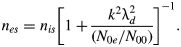
The Landau damping coefficient for IAW is given by (Krall & Trivelpiece, Reference Krall and Trivelpiece1973)

(10)

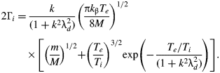
where T _e and T _i are electron and ion temperatures, V _is is the ion fluid velocity, λ_d = (k _bT ₀/4πN ₀₀e ²)^1/2 is the Debye length, and v _thi = (k _bT _i/M)^1/2 is the thermal velocity of ions. Combining Eqs. (6), (7), and (9) and assuming that the plasma is cold i.e., v _thi² ≪ c _s², one obtains the general equation governing the ion density variation

(11)

where c _s = (k _βT _e/M)^1/2 is the speed of the IAW for T _e ≫T _i. The solution of the above equation can be written as

(12)

here s is the Eikonal for IAW. The frequency and wave number of the IAW satisfy the following dispersion relation in the presence of laser beam

(13)

Substituting Eq. (12) into Eq. (11) and separating the real and imaginary parts, one obtains, the real part as

(14a)

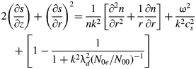
and imaginary part as

(14b)

To solve the coupled Eqs. (14a) and (14b), we assume the initial radial variation of IAW density perturbation to be Gaussian, and the solution at finite z may be written as

(15a)

and

(15b)

where k _i = Γ_i/kc _s², is the damping factor, f is a dimensionless beam width parameter and a is the initial beam width of the acoustic wave. We have used the following boundary conditions: df/dz = 0, f 1 at z = 0. Using Eq. (15) in Eq. (14a) and equating the coefficients of r ² on both sides, we obtain the following equation governing f

(16)

where R _d = ka ² is the diffraction length of the IAW. Eq. (16) represents the density profile of IAW in the plasma when the coupling between self-focused (filamented) laser beam and IAW is taken into account. It is interesting to compare Eq. (16) with Eq. (5), i.e., self-focusing of laser pump wave. In the absence of the coupling between the laser beam and acoustic wave, the second term in Eq. (16) is zero and the solution of Eq. (16) is given by

Thus, propagating a distance R _d, the width a is enlarged by and the axial amplitude of density perturbation in IAW is decreased by the same factor even in the absence of Landau damping.

We can, however, obtain an analytical solution of Eq. (16) in special case. When the laser beam has the critical power for self-focusing, the diffraction term (the first term on the right-hand-side of Eq. (5)) balances the nonlinear term in Eq. (5). Under such conditions (f ₀ = 1), the main beam propagates without convergence and divergence and is generally known as the uniform waveguide mode. Therefore, the solution for f is given by

where

Therefore, the amplitude of IAW (given by Eq. (15a)), which depends on f will be oscillating with z due to this nonlinear coupling, hence the IAW gets localized.

When the power of laser beam is greater than the critical power for self-focusing, we have solved Eq. (15a) numerically with the help of Eq. (16) to obtain the density perturbation at finite z. The result is shown in Figure 73a, for typical laser parameters as we have used in previous section. It is evident from the figure that the IAW gets excited due to nonlinear coupling with the high power laser beam because of the ponderomotive nonlinearity. If we take the zero Landau damping of IAW, we get the structure having the amplitude varying periodically with the z coordinate as shown in Figure 73c.

Fig. 73.

(Color online) Variation in IAW intensity with normalized distance (ξ = z/R _d0) and radial distance (r), for a =19 µm, (a) with Initial Landau damping (Γ_i/ ) = 0.0142 (b) with modified Landau damping (Γ_i/ ) = 0.0155, (c) with zero Landau damping.

The localization may be understood as follows: Because of the ponderomotive force exerted by the pump laser beam, the electrons are redistributed from the axial region. According to the dispersion relation ω² = k ²c _s²/(1 + k ²λ_d²(N _0e/N ₀₀)⁻¹), the phase velocity /k of the acoustic wave has a minimum on the axis and is increasing away from the axis. If we consider the initial wavefront of the electrostatic wave, the secondary wavelets travel with minimum velocity along the axis and with higher velocity away from the axis. As the wavefront advances in the plasma, focusing occurs, and the amplitude of the density perturbation increases. When the size of the wave front reduces considerably, diffraction effects also become important and hence the amplitude of the density perturbation starts to decrease.

We can calculate the periodicity length L of localized structures by putting r = 0 in Eq. (15a), as shown in Figure 74. According to Figure 74, value of L comes out to be 2.62R _d0. If we take the fast Fourier transform of the structure as shown in Figure 74, we get the spectral lines in one structure at a separation of k _A = 2π/L, and the value of k _A is coming out to be 2.4 R _d0⁻¹. We have shown these structures in Figure 75a. These periodic localized structures are similar to the structures in a periodic potential well. This situation can be modeled by representing Eq. (11) in the form of Mathew's equation in a periodic potential well. Therefore, taking the density variation as e ^it in Eq. (11), one can write

(17)

here,

(18)

where μ represents the dimensionless amplitude of the density perturbation in k-space. The normalized density of the first spectral component in Figure 75a is 5.801, which is at a distance of k _A from the central component. The value of μ² comes out to be μ² = (N _k²/N ₀₀²) = 0.0058, in which we have used the seed value of IAW (N ₀²/N ₀₀²) = 10⁻³. If n _is is of the form, n _is = ψexp(-i ʃ₀^T dτΛ), then we may write Eq. (17) in the form of Eigen value equation (Rozmus et al., Reference Rozmus, Sharma, Samson and Tighe1987)

(19)

Fig. 74.

(Color online) Variation in IAW intensity with normalized distance (ξ) in real space at r = 0 corresponding to Figure 73.

Fig. 75.

(Color online) Comparison of Power spectrum of IAW, for a E ²₀₀ = 1.6 (a) with Initial Landau damping (Γ_i/ϖ) = 0.0142 (b) with modified Landau damping (Γ_i/ϖ) = 0.0155.

We assume the solution of Eq. (19) in the form of Bloch wave function as

(20)

Substituting this solution in Eigen value Eq. (19), we obtain the equation

(21a)

and

(21b)

where

Keeping only ψ₀, ψ_±1 components, we obtain (Rozmus et al., Reference Rozmus, Sharma, Samson and Tighe1987) for Λ = Λ₁ + iΛ₂,

(22)

where the effective dampin _L is

(23)

and mismatch factor has the form

(24)

Eqs. (22) and (23) give the expression for modified frequency and enhanced Landau damping of the IAW, respectively. The value of the enhanced Landau damping is 0.0155, whereas the initial damping value was 0.0142. Therefore, we have approximately 10% increment in Landau damping of IAW, and the mismatch factor in Eigen frequency is coming out to be 0.0338. It is obvious that Landau damping governs the intensity of the IAW, and due to localization of IAW, the effective damping of the acoustic wave increases, therefore, as a result, the intensity of IAW reduces accordingly, as shown in Figure 73b. The enhanced Landau damping effect is also observable in the modified spectra of the IAW, as shown in Figure 75b.

13.4. Stimulated Brillouin Scattering

The high frequency electric field E _T, satisfies the wave equation

(25)

where J _T is the total current density vector in the presence of the high frequency electric field E _T and it is given by

(26)

E _T may be written as the sum of the electric field E of the pump laser beam and of the electric field E _S of the scattered wave, i.e.,

(27)

Substituting Eqs. (26) and (27) into Eq. (25), and separating the equation for pump and scattered field.,

(28a)

(28b)

In solving Eq. (28b), the term ∇(∇ × E _T) may be neglected in the comparison to the ∇²E _S term, assuming that the scale length of variation of the dielectric constant in the radial distance is much larger than the wavelength of the pump wave. Substituting v _t = (ieE/mω₀) in Eq. (28b), one obtains

(29)

let the solution of Eq. (29) be

(30)

where k _S0² = (ω_S²/c ²)(1 − (ω_p²/ω_S²)) = (ω_s²/c ²)ɛ_S0 and k _s1 and _s satisfy the matching conditions

Using Eq. (30) in Eq. (29), one gets

(31)

(32)

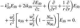
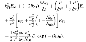
to a good approximation, the solution of Eq. (32) may be written as

(33)

substituting this into Eq. (32), one obtains

(34)

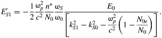
Simplifying Eq. (31) and substituting E _S0 = E _S00e ^iks0Sc, one obtains after separating the real and imaginary parts

(35a)

(35b)

The solution of these equations may again be written as

(36a)

(36b)

where b is the initial beam width of the scattered wave. Substituting the above solution in Eq. (35a) and equating the coefficients of r ² on both sides, we get the equation of the spot size of scattered wave as

(37)

where R _dS = k _S0b ² is the diffraction length of the scattered radiation.

It is easy to see from Eq. (15) that the IAW is damped as it propagates along the z-axis. Consequently, the scattered wave amplitude should also decrease with increasing z. Therefore, expressions for B' and b may be obtained on applying suitable boundary conditions E _S = E _S0exp(ik _S0z) +E _S1exp(−ik _S1z) = 0 at z = z _c; here z _c is the point at which the amplitude of the scattered wave is zero. This immediately yields

(38)

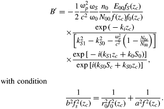
The reflectivity is defined as the ratio of scattered flux and incident flux, R = (|E _S|²/|E ₀₀|²). By using Eqs. (30), (33), (34), (36), and (38), we get E _SE*_S = E _S0E* _S0 +E _S0E* _S1 exp[i(k _S0+k _S1)z]+E _S1E* _S0 exp[−i(k _S0+k _S1)z] +E _S1E* _S1 and

(39)

It is apparent from the above equation that the reflectivity is dependant on the intensity of IAW and damping factor. To observe the effect of localization of IAW on SBS reflectivity, we have included the expression of modified Eigen frequency, (Eq. (22)) and effective damping, (Eq. (23)) in the above equation. It is clearly evident from Figure 76 that the SBS reflectivity gets reduced in the presence of the new Eigen frequency and damping values by almost the same factor as the intensity of the IAW decreases. In Figure 76, the solid red line (online only) shows the reflectivity with initial damping value and the dashed blue line (online only) shows the reflectivity including the effective enhanced Landau damping. If we calculate the integrated SBS reflectivity in two cases: namely (1) with initial damping of IAW and (2) with modified enhanced damping of IAW, we find that the reduction in SBS reflectivity comes out to be approximately 10%.

Fig. 76.

(Color online) Variation in normalized back scattered reflectivity of SBS, |Es|²/|E ₀₀|² with normalized distance, (a) when (Γ_i/ϖ) = 0.0142 (solid red line) and (b) when (Γ_i/ϖ) = 0.0155 (blue dashed line).

ACKNOWLEDGMENTS

This work was partially supported by DST, Government of India. One of the authors (Prerana Sharma) is grateful to AICTE India for providing financial assistance. One of the authors (Shivani) is grateful to Dr. R. Uma for useful discussions.

14.1. Introduction

Stimulated Brillouin scattering (SBS) optical phase conjugation (OPC), a technique with profound significance to high-power laser science, has been studied and made great efforts to application practically by researchers all over the world for decades (Zel'dovich et al., Reference Zel'dovich, Popovichev, Ragulsky and Faizullov1972; Basov & Zubarev, Reference Basov and Zubarev1979; Meister et al., Reference Meister, Riesbeck and Eichler2007; Ostermeyer et al., Reference Ostermeyer, Kong, Kovalev, Harrison, Fotiadi, Megret, Kalal, Slezak, Yoon, Shin, Beak, Lee, Lu, Wang, Lin, Knight, Kotova, Straber, Scheikhobeid, Riesbeck, Meister, Eichler, Wang, He, Yoshida, Fujita, Nakatsuka, Hatae, Park, Lim, Omatsu, Nawata, Shiba, Antipov, Kuznetsov and Zakharov2008). In demand for large laser engineering such as inertial confinement fusion and inertial fusion energy, works on SBS phase conjugator, SBS beam combiner, and so on, are being carried out by more and more research teams (Kong et al., Reference Kong, Lee and Lee2005c, Reference Kong, Yoon, Shin, Beak and Lee2006, Reference Kong, Yoon, Beak, Shin, Lee and Lee2007b, Reference Kong, Yoon, Shin and Beak2008, Reference Kong, Shin, Yoon and Beak2009a; Kappe et al., Reference Kappe, Strasser and Ostermeyer2007; Hasi et al., Reference Hasi, Lu, Li and He2007, 2008d; Wang et al., Reference Wang, Lu, Lin, Ding and Jiang2007, Reference Wang, Lu, He, Zheng and Zhao2009a; Yoshida et al., Reference Yoshida, Fujita, Nakatsuka, Ueda and Fujinoki2007). As well known, advantages of the SBS phase conjugator are high energy-conversion efficiency and simple structure. However, the acoustic wave, which plays a crucial role in SBS process, is developed from the noise in Brillouin medium (Boyd et al., Reference Boyd, Rzazewski and Narum1990), which makes the phase conjugate wave instable in many situations. For instance, phase jumps or intensity modulations are frequently observed in experiments (Shahraam et al., Reference Shahraam, Vladimyros and Jesper1998; Yang et al., Reference Yang, Yang, Ding, Li, Zhang and Mang2001), and when the leading-edge of the laser pulse is shorter than or comparable with the phonon lifetime of the Brillouin medium, SBS phase-conjugate fidelity and its stability will deteriorate severely (Dane et al., Reference Dane, Neuman and Hackel1992), which keeps this technique far away from applications of short pulse such as fast ignition laser pulse. Besides, the Stokes wave competes with optical noise modes throughout its generation and amplification processes, leading to the existence of non-conjugate components of the output wave, that is to say, and the phase-conjugate fidelity can never really achieve 100% (Zel'dovich et al., Reference Zel'dovich, Pilipetskii and Shkunov1982). So far as it goes, problems mentioned above, whose root is the noise-origin characteristic of the acoustic wave, have severe limiting factors for practical application of SBS phase conjugator.

There is another OPC technique, called Brillouin enhanced four-wave mixing (BEFWM), which is also based on acousto-optic interaction, but different from SBS in acoustic origin mechanism in nature (Scott & Ridley, Reference Scott and Ridley1989). In BEFWM process, acoustic wave is driven by optical coherent beating patterns and built up instantaneously without acoustic-relaxation-time restriction of the medium. This non-noise process not only keeps OPC stable and transient-state-adaptable but also exhibits advantages as non-threshold and a 100% conjugate fidelity. In the past decades, researches on BEFWM mainly focused on the conjugate-amplification of weak optical signals, and have gain many achievements (Andreev et al., Reference Andreev, Bespalov and Dvoretsky1989; Lanzerotti et al., Reference Lanzerotti, Schirmer and Gaeta1996; Zhu et al., Reference Zhu, Lu, He, Ba, Wang, Gao and Dong2007). However, when BEFWM operates with large incident signals as a high-power phase conjugator, its efficiency, i.e., total reflectivity, will be low because the energy of the conjugate wave comes from the reference wave instead of the signal wave itself (Zhu et al., Reference Zhu, Lu, He, Guan and Xu2008).

In this work, a composite phase conjugator scheme, in which mechanism of BEFWM and SBS are combined in a compact structure is reported. The BEFWM provides phase conjugate wave seed with fast response, high quality and stability, which is then magnified by stimulated Brillouin amplification (SBA) with high energy-conversion efficiency. As a result, advantages of BEFWM and SBS can be realized at the same time. In the following sections, the theoretical model is set up, as well as numerical simulations, and demo experiments are carried out. Feasibility of the BEFWM-SBA phase conjugator is verified sufficiently.

14.2. Theory

14.2.1. Physical Model

Physical model of the BEFWM-SBA composite phase conjugator is shown in Figure 77. E ₁ and E ₂, in Figure 77a, are counter-propagating reference waves, while E ₂ has a relative Stokes-shift in frequency. The laser signal wave E ₃, as the main laser wave whose power is much greater than the reference waves, intersects E ₁ at a small angle, and its conjugate wave generated by the phase conjugator is termed as E ₄. All the input waves should be linearly polarized, among which E ₁ is in p-polarized-state, E ₂ is in s-state, and let the polarized direction of E ₃ be slanted slightly, so as to share its power in s-state for a little and most of them be contained in p-state.

Fig. 77.

Physical model of the composite-mechanism phase conjugator scheme.

In order to describe these polarization states more explicit, we add letters p and s to the wave notations in Figure 77b, and term the two polarized components of E ₃ as E _3p and E _3s separately. The physical picture of interaction among these waves can be depicted as follows: when encountering in the Brillouin medium, s-state E _3s and E _2s interfere with each other and drive the periodic density variations in the medium that travels from left to right at a velocity close to the velocity of sound in the medium, thus an acoustic wave ρ_FWM with frequency Ω is produced as a result. ρ_FWM acts as a moving Bragg-phase grating, once founded, it will scatter E _1p and generate the p-state Stokes-shifted wave E _4p, which is phase conjugated with the laser signal E ₃. Then, as E _4p propagates opposite to the way of E ₃, it will be Brillouin-amplified by E _3p that is also in the p polarized direction, and high efficiency power growth can be realized.

There are two procedures existing in this scheme. At first, a phase conjugate wave seed is generated through Stokes-type polarization-decoupled BEFWM. Then, growth of the conjugate wave mainly depends on the SBA process. The former process provides characteristics for E ₄ as high stability and fidelity, the later one ensures high conversion efficiency. In this way, advantages of BEFWM and SBS can be realized in the composite phase conjugator at the same time.

However, when ρ_FWM is built, waves in all polarized states will be scattered by it immediately. According to the propagating direction of ρ_FWM, the signal component E _3p might be Stokes-scattered by ρ_FWM and generate a Stokes-shifted wave E _2p, which is conjugated with E _1p.We call E _2p a parasitic wave. Here come two harmful effects from the parasitic wave. First, power in E _3p will be lost partly, resulting in decrease of the Brillouin amplification gain of E _4p. Second, E _2p will be Brillouin amplified by E _1p and therefore reduce the E _1p power that should be transported into E _4p through BEFWM process. So, how to ensure that E _4p have the dominance over E _2p during all the processes of generation and amplification is an important issue for this conjugator scheme.

14.2.2. Mathematical Model

In the following mathematical model, the acoustic waves of SBA in two different directions, i.e., E _3p versus E _4p and E _1p versus E _2p, are denoted as ρ₃₄ and ρ₁₂, respectively, which propagate from left to right too. All of the six optical waves can be described by Maxwell's wave equations, and the three acoustic waves can be depicted by Navier-Stokes's energy transmission equation. Taking the interaction geometry into account as shown in Figure 77b and based on the assumption of neglecting in the second derivations, the nonlinear coupled-equations describing all the processes mentioned above along the z direction can be written as

(1)

(2)

(3)

(4)

(5)

(6)

(7)

(8)

and

(9)

where E and ρ are amplitudes of optical and acoustic wave, respectively; c is light velocity in the vacuum; n denotes the refractive index; g _a(θ) is the acoustic coupling coefficient with the angle θ between the optical waves, and numerically equals to g _a cos²(θ/2) (Aschroeder et al., Reference Aschroeder, Damzen and Hutchinson1989), in which g _a is the value for θ = 0; Γ_B is the Brillouin line width of the medium; ΔΩ = Ω (cos(θ/2)−1) and Δk = nΩ(cosθ − 1)/c represent, respectively, the frequency detuning and the phase mismatch of acoustic waves in BEFWM; α is the optical absorption coefficient. Compared with the light velocity, the sound velocity is so small that the propagation terms have been neglected in the three acoustic waves, Eqs. (7–9).

According to Figure 77b, E _1p, E _3p, and E _3s are injected at z = 0 while E _2s at z = L ₂. E _4p and E _2p equal to zero at z = L ₂ or when t = 0. Intensities of other optical waves will be specified as demand. Interaction length of BEFWM is limited between L ₁ and L ₂, and where out of this range, the gain of BEFWM equals to zero. Brillouin amplifications exist in the entire space 0 ~ L ₂ along the propagation directions of E ₁ and E ₃. So far, all the boundary and initial conditions of the equations are defined, and the numerical simulation can be carried out.

14.2.3. Simulation and Analysis

In the numerical simulation, the laser signal is chosen as 1.06-μm wavelength and 20-ns full width at half maximum Gaussian pulses. CS₂ is chosen as the Brillouin medium (Hasi et al., Reference Hasi, Lu, He and Wang2005), whose n = 1.59, SBS gain coefficient is 68 cm/GW, the phonon lifetime is 6.4 ns, and α = 4 ×10⁻³cm⁻¹. Besides, we set the parameters as: L ₁ = 35 cm, L ₂ = 50 cm, θ = 10 mrad, the peak intensity ratio of the reference waves is |E _1p|²:|E _2s| ² = I _1p:I _2s = 2, and the peak intensity ratio of the two polarization components in the signal E ₃ is |E _3p|²:|E _3s| ² = I _3p:I _3s = 20:1.

As mentioned above, suppression of the parasitic wave E _2p is important. An effective method to realize it is to decrease I _1p comparing with I _3p, i.e., to decrease the pumping intensity in the SBA process of the parasitic wave E _2p, so as to decrease the energy extraction ratio for E _2p from E _1p. To do this, although the initial intensity of E _4p generated in BEFWM will be weaker, it can be amplified to become a considerable magnitude by the high-intensity pump wave E _3p in the following SBA process. In Figure 78a, the simulating input pulse waveforms of E _1p, E _3p, and the output waveforms of E _4p and E _2p are shown in the same intensity scale when the injected peak intensities I _3p = 50 MW/cm² and I _1p = 5 MW/cm². It is easy to demonstrate that the output E _2p is rather weak.

Fig. 78.

(Color online) Numerical simulation on the input and output waveforms of the conjugator when the incident peak power I _3P = 50MW/cm², I _1P  = 5 MW/cm², without signal delay (a), and with 20-ns signal delay (b).

Another method helping to suppress the E _2p pulse is to set injecting temporal delay for E ₃ relative to E ₁ pulse, through which, when E ₃ arrives in the BEFWM region and E _2p is generated, there is only a tail part of the E _1p pulse to provide energy transferring to E _2p in the SBA process, which is very limited in energy and actuation duration. Nevertheless, if only the conjugate wave seed E _4p is generated, even though its duration of generation is short and intensity is weak, it can be amplified during the whole subsequent signal pulse span with a high gain. In Figure 78b, it is set as I _1p = 5 MW/cm², I _1p = 50 MW/cm², and E ₃ is delayed by 20 ns relative to E ₁. It can be seen that peak intensity of the conjugate pulse E _4p is close to 50 MW/cm², while E _2p can almost be neglected.

Other parameter-contributions to the composite PC have been calculated numerically in our theoretical simulation work, and feasibility of this composite-mechanism scheme is verified in the theory. Performance of the PC, such as reflectivity will be discussed in the next section.

14.3. Experiments

14.3.1. Experimental Setup

The experimental setup is shown in Figure 79. The Nd:YLF single frequency TEM₀₀ Q-switched laser, operating at 1-Hz repetition rate, can deliver about 120 mJ p-polarized-state pulses at 1053 nm in a 20-ns full width at half maximum quasi-Gaussian pulse shape. The beam diameter is about 4 mm. A λ/2 plate and polarizer P ₁ are used to split the laser beam into E ₁ wave, i.e., E _1p, and E ₃ wave. After passing through the 4% sampling plate SP₁ and the polarizer P ₄, E _1p enters the 80-cm-length composite cell filled with CS₂, i.e., Cell-1, and the forepart of E _1p pulse that transmitted throughout of Cell-1 generates backward Stokes wave in a short-focused-type SBS CS₂ cell, i.e., Cell-2, whose lens focus equals to 10 cm and distance from Cell-1 is about 70 cm. When passing backward through the λ/4 plate, the Stokes wave is changed into s-polarized state, then enters into the back window of Cell-1, and acts as E _2s. The E ₃ wave, which is reflected by the polarizer P ₁ and then by P ₂ turns into p-polarized state by a 45° rotor and a 45° Farady rotator, and penetrates through the polarizer P ₃ entirely. Then it is adjusted by a λ/2 plate to contain a small s-state component with ratio of I _3p/I _3s = 20, and coupled by 20-ns delay mirrors M₁–M₆ into Cell-1 where BEFWM-SBA process is built up. The angle between E ₁ and E ₃ is about 10 mrad. The penetrated part of E ₃ is obstructed by a diaphragm set behind Cell-1. The conjugate wave E _4p generated in Cell-1 propagates backward along the way of E ₃, and finally penetrates P ₂ to become the output wave. The residual E _2s and the parasite wave E _2p will propagate backward along the way of E ₁. E _2s will be reflected off by the polarizer P ₄, and E _2p can be blocked by the isolator.

Fig. 79.

Experimental setup of the BEFWM-SBA phase conjugator in demo-version.

In the experiments, we recorded the injection E _1p and the output of E _2p on the two sides of SP₁, and recorded E ₃ and E _4p on SP₂ simultaneously. In order to simulate high-flux laser system, a long focus lens with f = 300 cm is inserted in the path of E ₃ to increase the signal intensity to a certain extent in the BEFWM-SBA region, while the focus of the 300-cm lens is located out of the Cell-1 in order to avoid self excitational SBS of E3.

14.3.2. Results and Discussion

Pulsed waveforms and near-field intensity patterns of the input signal E ₃ and the output conjugate wave E ₄ measured in experiments are shown in Figure 80. A little step, which is usually observed in the Brillouin amplification process, is shown at the root of E ₄ waveform. Consistency of the in and out beam cross-sectional patterns is achieved well.

Fig. 80.

(Color online) Pulsed waveforms and near-field intensity patterns of the input signal wave E ₃ and the output conjugate wave E ₄.

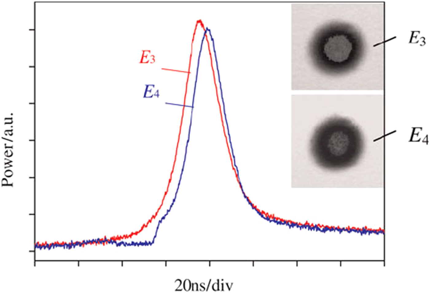
In order to research the performance of the composite phase conjugator with different laser signal power, in the experiments, we fixed the incident E ₁ at 8 mJ/pulse, and varied E ₃ from 6 mJ/pulse to about 82 mJ/pulse gradually by changing the applied voltages charged on the Xe-lamps of the Nd:YLF laser. It is shown that the output E ₄ increases from about 3 mJ/pulse to about 61 mJ/pulse, while the parasitic E _2p is kept in a range between about 3 mJ/pulse and 6 mJ/pulse, as shown in Figure 81.

Fig. 81.

Output pulse energies of E ₄ and E _2P with different incident laser signal E ₃.

Reflectivity R of the composite phase conjugator is defined as energy ratio of E ₄ and E ₃ pulses, i.e., R = E ₄/E ₃, which have been measured synchronously using the two same calorimeters at both sides of the sampling plate SP₂. For each measuring point, we recorded pulse energies continuously for 60 shots, and analyzed the mean value of R and its shot-to-shot fluctuations. In the discussion about, the stability of the conjugator, fluctuations of the laser itself should be taken into account, because variations in the signal can induce the change of R correspondingly. We note the relative instability of R with the symbol β, and calculate it by

where the symbol with bar on the head is the mean value at a certain measuring point, and Δ denotes the standard deviation, i.e., root mean square. Figure 82a shows the experimental results of R which is as a function of E ₃. The increase of E ₃ induced the growth of R from 55% to a saturation value about 75%. β is shown in Figure 82b. It is seen that β is almost fixed within the range close to or below 1% during the whole variation of E ₃ and at any R values, which demonstrates a very good stability.

Fig. 82.

Reflectivity R (a) and its relative instability β (b) with different incident laser signal E ₃.

In Figure 82a, the theoretical result is shown as a solid line. Although the tendency of which is in accordance with the experiments, it is seen obviously that the deviation occurs when E ₃ is larger. In our analysis, it is attributed to incomplete polarization control for the injecting optical waves.

Far-field divergence angles of the output conjugate wave E ₄ is recorded by an array camera, the result is shown in Figure 83. When the signal increases, the mean value of the divergence angles of E ₄ is about 0.451 mrad, which is close to the signal divergence 0.434 mrad. In addition, the fluctuation of the output divergence angles is below 5% in the whole experimental signal range.

Fig. 83.

Far-field divergence angles of the output conjugate wave E ₄ with different incident laser signal E ₃.