1 Introduction
The upper ocean is humming with fluid dynamical phenomena. Submesoscale currents, boundary-layer turbulence, inertia–gravity waves and surface gravity waves evolve together even under larger-scale forcing conditions, leading to a rich collection of coherent structures with multiple time and space scales (see the review by McWilliams (Reference McWilliams2016)). In the submesoscale range, a regime with horizontal length scales [0.1–10] km, surface images and numerous high resolution computational solutions find fronts, vortices and dense filaments are dominant flow structures. Of particular interest here are the thin elongated filaments, or surface convergence lines, which frequently form in the spiral bands of larger structures, for example see the images in McWilliams, Colas & Molemaker (Reference McWilliams, Colas and Molemaker2009a
, figure 1), Gula, Molemaker & McWilliams (Reference Gula, Molemaker and McWilliams2014, figure 4), and McWilliams (Reference McWilliams2016, figures 2 and 6). Cold dense filaments, essentially a closely coupled pair of warm–cold cold–warm fronts that overlap in the cold region, are highly anisotropic structures with a horizontal extent of kilometres and a length-to-width aspect ratio
 $\gg 10$
or more. These filaments are dynamically important, they can undergo explosive strain-induced frontogenesis, i.e. intense sharpening of their horizontal buoyancy and current gradients in a short time of the order of hours (McWilliams, Molemaker & Olafsdottir Reference McWilliams, Molemaker and Olafsdottir2009b
). Cold filament frontogenesis (CFF) is thus an extremely efficient pathway for transferring energy to smaller scales (Lapeyre & Klein Reference Lapeyre and Klein2006; McWilliams et al.
Reference McWilliams, Colas and Molemaker2009a
; Gula et al.
Reference Gula, Molemaker and McWilliams2014). CFF thus serves as an efficient bridge in the energy cascade between ocean mesoscale eddies and small-scale dissipative motions.
The nonlinear couplings between surface waves, boundary-layer turbulence and submesoscale motions that impact frontogenesis is speculated to be tight based on simplified conservative dynamics. A more complete picture of the interacting processes incorporating turbulence dynamics is just beginning to be unravelled, but impediments persist because of the wide disparity in time and space scales that need to be resolved by turbulence simulation codes. Previously, Sullivan & McWilliams (Reference Sullivan and McWilliams2018, hereafter referenced as SM18) used large-eddy simulation (LES) to carry out process studies examining the life cycle of CFF for varying surface forcing, down-filament winds, across-filament winds and surface cooling, all without surface waves. Starting from fully developed boundary-layer turbulence, all solutions exhibit a CFF life cycle, and they find the frontal arrest mechanics are primarily from a lateral shear instability. At arrest, the collapsed frontal width
 ${\sim}100~\text{m}$
, and the horizontal current gradients generate very large horizontal variances and momentum flux
 $\langle v^{\prime 2},u^{\prime 2},u^{\prime }v^{\prime }\rangle$
; for example, at the water surface with down-filament winds the turbulent kinetic energy (TKE) normalized by friction velocity
 $u_{\ast }$
is
 $\text{TKE}/u_{\ast }^{2}\sim 40$
with peak Rossby number
 $Ro\sim 88$
. Also, they find quantitative differences depending on the wind direction and surface stress and buoyancy forcing.
The present article builds on SM18 and investigates the coupling between wavy upper ocean boundary-layer turbulence, so-called Langmuir turbulence (McWilliams, Sullivan & Moeng Reference McWilliams, Sullivan and Moeng1997), and a single submesoscale cold density filament using high Reynolds number LES based on wave-averaged dynamical equations (Craik & Leibovich Reference Craik and Leibovich1976; Holm Reference Holm1996; McWilliams, Restrepo & Lane Reference McWilliams, Restrepo and Lane2004). In particular, we examine the role of turbulence, surface waves and secondary circulations (SC) in CFF, and their impact on the lateral shear instability that leads to arrest. It is now well documented that the Stokes-drift ‘vortex force’ generates coherent structures, namely Langmuir circulations, in homogeneous boundary layers in a variety of stratified flow regimes. However, the possible impact of vortex forces in the submesoscale regime examined here is open for exploration. There is a growing database of literature related to aspects of the present work. Skyllingstad & Samelson (Reference Skyllingstad and Samelson2012), Thomas & Lee (Reference Thomas and Lee2005) and Pham & Sarkar (Reference Pham and Sarkar2018) all use LES to study the evolution of submesoscale filaments, but with no surface waves. McWilliams & Fox-Kemper (Reference McWilliams and Fox-Kemper2013) derive wave-averaged balance relations for fronts and filaments showing Stokes forces enter balance dynamics sooner than finite Rossby effects
 $Ro<1$
which hints that wave effects are potentially important in the mesoscale and submesoscale regime. In a series of papers, McWilliams et al. (Reference McWilliams, Gula, Molemaker, Renault and Shchepetkin2015), McWilliams (Reference McWilliams2017, Reference McWilliams2018) examined boundary-layer-induced frontogenesis for filaments and one-sided fronts using the vertical mixing scheme K-Profile Parameterization (KPP) (Large, McWilliams & Doney Reference Large, McWilliams and Doney1994) including surface wave effects. Also, in their analysis of the LES by Hamlington et al. (Reference Hamlington, Van Roekel, Fox-Kemper, Julien and Chini2014), Suzuki & Fox-Kemper (Reference Suzuki and Fox-Kemper2016), Suzuki et al. (Reference Suzuki, Fox-Kemper, Hamlington and Roekel2016) find surface waves impact the momentum budgets and frontogenesis at late times in the spindown from an initially nearly quiescent warm filament. The one-sided front analysed at a single late time snapshot is oriented in the down-front Stokes-drift direction with
 $Ro\sim 3$
; they find one-sided fronts oriented down the Stokes-drift direction are stronger. Using a combination of analytic theory and numerical simulations Li et al. (Reference Li, Zhang, Chini and Flierl2012) and Haney et al. (Reference Haney, Fox-Kemper, Julien and Webb2015) find that down-front surface waves alter the linear stability of submesoscale fronts in thermal wind balance due to the Craik–Leibovich vortex force. Smith, Hamlington & Fox-Kemper (Reference Smith, Hamlington and Fox-Kemper2016) finds ocean tracers are impacted by the coupling between submesoscale turbulence and surface waves.
It is important to mention that surface winds driving a cold dense filament and a single-sided front (e.g. Suzuki et al.
Reference Suzuki, Fox-Kemper, Hamlington and Roekel2016) are fundamentally different turbulent flows (McWilliams Reference McWilliams2018). Compared to a one-sided front, a warm–cold–warm density filament features stronger frontogenesis (McWilliams et al.
Reference McWilliams, Molemaker and Olafsdottir2009b
) and two opposite signed baroclinic jets
 $v_{j}$
. Down-filament surface winds and waves with Stokes drift
 $v^{s}>0$
are then simultaneously up-front and down-front relative to the underlying baroclinic jets, i.e. on the west and east sides of the filament
 $v^{s}\cdot v_{j}<0$
and
 $v^{s}\cdot v_{j}>0$
, respectively. Surface winds aligned with a one-sided front are either up-front or down-front but not both. The impact of waves and wave direction on CFF at large Rossby number is relatively unknown and results from one-sided fronts cannot be linearly superimposed and extrapolated to filaments.
The theory of boundary-layer-induced frontogenesis does not explain the turbulent arrest and decay dynamics nor the role of surface gravity waves. Thus, the perspective of this paper is primarily on submesoscale phenomenology with surface waves. The roadmap of the manuscript is as follows: a brief description of the LES equations and numerical algorithm is given in § 2, an outline of the numerical experiments is in § 3, the analysis technique used to decompose flow variables and the concept of a turbulent thermal wind (TTW) with wave effects is described in § 4, with results for down-filament/across-filament waves discussed in §§ 5 and 6, respectively. A summary of the findings is given in § 7.
2 Large-eddy simulation
The dynamics of the upper ocean boundary layer (OBL), including submesoscale and boundary-layer motions, is assumed to be governed by wave-averaged equations first proposed by Craik & Leibovich (Reference Craik and Leibovich1976) with later extensions described by McWilliams et al. (Reference McWilliams, Sullivan and Moeng1997, Reference McWilliams, Restrepo and Lane2004). Our LES model for the OBL is based on the original Craik–Leibovich equations in the ‘vortex force’ representation, i.e. the momentum equations include an additional vortex force
 $\boldsymbol{u}^{s}\times \unicode[STIX]{x1D74E}$
where
 $\boldsymbol{u}^{s}$
is the Stokes drift of the wave field and
 $\unicode[STIX]{x1D74E}=(\unicode[STIX]{x1D709},\unicode[STIX]{x1D702},\unicode[STIX]{x1D701})$
is the vorticity vector. We further assume a Boussinesq fluid and thus the LES equation set with system rotation and stable stratification is
 $$\begin{eqnarray}\displaystyle \displaystyle \frac{D\boldsymbol{u}}{\unicode[STIX]{x2202}t} & = & \displaystyle -\boldsymbol{f}\times (\boldsymbol{u}+\boldsymbol{u}^{s})-\unicode[STIX]{x1D735}\unicode[STIX]{x03C0}+b\hat{\boldsymbol{z}}+\boldsymbol{u}^{s}\times \unicode[STIX]{x1D74E}-\unicode[STIX]{x1D735}\boldsymbol{\cdot }\boldsymbol{T}\end{eqnarray}$$
 $$\begin{eqnarray}\displaystyle \displaystyle \frac{Db}{\unicode[STIX]{x2202}t} & = & \displaystyle -\boldsymbol{u}^{s}\boldsymbol{\cdot }\unicode[STIX]{x1D735}b-\unicode[STIX]{x1D735}\boldsymbol{\cdot }\boldsymbol{B}\end{eqnarray}$$
 $$\begin{eqnarray}\displaystyle \displaystyle \unicode[STIX]{x1D735}\boldsymbol{\cdot }\boldsymbol{u} & = & \displaystyle 0.\end{eqnarray}$$
 $\unicode[STIX]{x1D70C}\boldsymbol{u}$
and (2.1b
) for buoyancy
 $b$
. The divergence free (incompressible) condition (2.1c
) determines the elliptic pressure variable
 $\unicode[STIX]{x03C0}$
. Variables that appear in (2.1) are as follows: velocity components
 $\boldsymbol{u}\equiv u_{i}=(u,v,w)$
, rotation vector
 $\boldsymbol{f}=(0,0,f)$
with
 $f$
the Coriolis parameter and unit vector
 $\hat{\boldsymbol{z}}$
in the vertical direction. The buoyancy variable is defined in terms of water density:
 $b=g(\unicode[STIX]{x1D70C}_{o}-\unicode[STIX]{x1D70C})/\unicode[STIX]{x1D70C}_{o}$
where
 $(\unicode[STIX]{x1D70C},\unicode[STIX]{x1D70C}_{o})$
are density and reference density, respectively. We assume a linear equation of state connects temperature
 $\unicode[STIX]{x1D703}$
and density:
 $\unicode[STIX]{x1D70C}=\unicode[STIX]{x1D70C}_{o}[1-\unicode[STIX]{x1D6FD}(\unicode[STIX]{x1D703}-\unicode[STIX]{x1D703}_{0})]$
with
 $\unicode[STIX]{x1D6FD}$
the coefficient of expansion and
 $\unicode[STIX]{x1D703}_{0}$
a reference temperature. The additional forcing from larger-scale submesoscale density fronts is implicit in the specification of the initial buoyancy field. In the vortex-force representation of the wave-averaged Boussinesq equations, the pressure variable
 $$\begin{eqnarray}\unicode[STIX]{x03C0}=\frac{p}{\unicode[STIX]{x1D70C}_{o}}+\frac{2e}{3}+\frac{1}{2}|\boldsymbol{u}+\boldsymbol{u}^{s}|^{2}-\frac{1}{2}|\boldsymbol{u}|^{2}\end{eqnarray}$$
includes pressure
 $p$
and a Bernoulli head from the subgrid-scale (SGS) energy
 $e$
and from Stokes drift (also see Holm Reference Holm1996; McWilliams et al.
Reference McWilliams, Sullivan and Moeng1997).
The LES equations contain SGS momentum and buoyancy fluxes
 $(\boldsymbol{T}\equiv \unicode[STIX]{x1D70F}_{ij},\boldsymbol{B}\equiv b_{i})$
, and SGS energy
 $e$
. We use eddy viscosity prescriptions
 $\unicode[STIX]{x1D70F}_{ij}=-\unicode[STIX]{x1D708}_{t}(\unicode[STIX]{x2202}u_{i}/\unicode[STIX]{x2202}x_{j}+\unicode[STIX]{x2202}u_{j}/\unicode[STIX]{x2202}x_{i})$
and
 $b_{i}=-\unicode[STIX]{x1D708}_{h}\unicode[STIX]{x2202}b/\unicode[STIX]{x2202}x_{i}$
described by Moeng (Reference Moeng1984) and Sullivan, McWilliams & Moeng (Reference Sullivan, McWilliams and Moeng1996). The turbulence eddy viscosities
 $(\unicode[STIX]{x1D708}_{t},\unicode[STIX]{x1D708}_{h})$
are parameterized in terms of
 $e$
,
 $(\unicode[STIX]{x1D708}_{t},\unicode[STIX]{x1D708}_{h})\sim \sqrt{e}\ell$
where the length scale
 $\ell$
is proportional to the grid mesh spacing
 $\unicode[STIX]{x0394}$
, but is reduced for strong stratification. To account for non-equilibrium effects at small scales we also solve an additional prognostic equation for
 $e$
; this SGS energy equation includes a standard suite of terms, production, buoyancy, diffusion and dissipation (Moeng Reference Moeng1984), and also includes advection by Stokes drift and Stokes production (McWilliams et al.
Reference McWilliams, Sullivan and Moeng1997; Sullivan et al.
Reference Sullivan, McWilliams and Melville2007b
).
The wave-averaged momentum equations can be cast in several alternative but mathematically equivalent representations using vector identities as shown by Holm (Reference Holm1996) and Suzuki & Fox-Kemper (Reference Suzuki and Fox-Kemper2016). The alternative form advocated by Suzuki & Fox-Kemper (Reference Suzuki and Fox-Kemper2016) utilizes the pressure variable
 $p$
, an advective Lagrangian velocity
 $\boldsymbol{u}^{L}=\boldsymbol{u}+\boldsymbol{u}^{s}$
and Stokes-shear forces
 $u_{j}^{L}\unicode[STIX]{x1D735}u_{j}^{s}$
; the notation reads
 $u_{j}^{L}=\boldsymbol{u}^{L}$
and
 $u_{j}^{s}=\boldsymbol{u}^{s}$
. Their formulation has numerous interesting interpretations, but the vortex-force formulation adopted here, in our opinion, offers an equally clear interpretation of the impact of surface waves on momentum and scalar transport, see §§ 4–6.
Details of the LES, including the SGS prescription, algorithmic details, and wave–current interaction terms are not repeated here. They can be found in SM18 with fuller explanations in numerous references (e.g. Moeng Reference Moeng1984; Sullivan, McWilliams & Moeng Reference Sullivan, McWilliams and Moeng1994; Sullivan et al. Reference Sullivan, McWilliams and Moeng1996; McWilliams et al. Reference McWilliams, Sullivan and Moeng1997; McWilliams, Moeng & Sullivan Reference McWilliams, Moeng, Sullivan and Geernaert1999; Sullivan et al. Reference Sullivan, McWilliams and Melville2007b ; Sullivan & Patton Reference Sullivan and Patton2011; Sullivan et al. Reference Sullivan, Romero, McWilliams and Melville2012; Moeng & Sullivan Reference Moeng, Sullivan, North, Zhang and Pyle2015).
3 LES experiments
The database of solutions in SM18 includes simulations of a submesoscale cold dense filament coupled to turbulent OBLs driven by surface winds or by surface cooling. We build on our previous work and carry out identically posed computational problems but now include phase-averaged wave–current interactions as described in McWilliams et al. (Reference McWilliams, Sullivan and Moeng1997). These LES experiments are not crafted as a case study of a specific submesoscale regime, but rather as a process study designed to expose the generic dynamics of cold filament frontogenesis in the presence of waves. The computational domain and mesh discretization are picked to match SM18 which allows a one-to-one comparison between simulations with and without surface wave effects. The imposed submesoscale filament is a two-dimensional (2-D) (
 $x$
–
 $z$
) varying strip with tapered horizontal edges and depth dependence so that it smoothly blends into the far field and the deeper thermocline. The filament horizontal scale
 $L=2~\text{km}$
(
 $1/2$
of the filament width), and the temperature jump between the far field and the cold filament centreline is approximately
 $-0.48\,^{\circ }\text{C}$
. The nominal depth of the filament is
 $h_{o}=-60~\text{m}$
. Specific formulas describing the spatial variation of the filament are given in the appendix of SM18.
The computational domain size is
 $(L_{x},L_{y},L_{z})=(12,4.5,-0.25)~\text{km}$
with discretization
 $(N_{x},N_{y},N_{z})=(8192,3072,256)\sim 6.4\times 10^{9}$
grid points. This corresponds to a horizontal spacing
 $\unicode[STIX]{x0394}x=\unicode[STIX]{x0394}y=1.46~\text{m}$
. The vertical grid is smoothly stretched with finer resolution near the water surface
 $\unicode[STIX]{x0394}z=[0.5{-}1.68]~\text{m}$
; the vertical spacing between neighbouring cells is increased by a constant stretching factor
 $K=\unicode[STIX]{x0394}z_{k+1}/\unicode[STIX]{x0394}z_{k}=1.0048$
, for
 $k=1,N_{z}$
. The size of the computational domain is picked to capture large-scale horizontally anisotropic motions and small-scale three-dimensional (3-D) turbulence during the life cycle of filament frontogenesis. Given the filament alignment in the computational box, the coordinates
 $(x,y,z)$
are also referred to as across-filament, down-filament and vertical directions. The origin of the
 $x$
axis is at the filament centreline,
 $x=[-6000,6000]~\text{m}$
.
Wind stress is applied in either the west-to-east or south-to-north directions with a water-side friction velocity
 $u_{\ast }=0.01~\text{m}~\text{s}^{-1}$
and zero surface cooling
 $Q_{\ast }$
. This wind stress corresponds to surface winds of
 $U=8.5~\text{m}~\text{s}^{-1}$
with a drag coefficient
 $C_{d}\sim 1.2\times 10^{-3}$
based on the relationship given by Large & Pond (Reference Large and Pond1981). To examine the impact of the surface forcing we conduct a third set of experiments with zero wind stress with surface cooling of
 $100~\text{W}~\text{m}^{-2}$
which equates to a kinematic surface flux
 $Q_{\ast }=2.38\times 10^{-5}~\text{K}~\text{m}~\text{s}^{-1}$
. The Deardorff (Reference Deardorff1972) convective velocity scale
 $w_{\ast }=(g\unicode[STIX]{x1D6FD}|h_{i}|Q_{\ast })^{1/3}=0.0137~\text{m}~\text{s}^{-1}$
, based on the initial boundary-layer depth
 $h_{i}=-66.5~\text{m}$
, coefficient of thermal expansion
 $\unicode[STIX]{x1D6FD}=1.668\times 10^{-4}~\text{K}^{-1}$
and gravity
 $g=9.81~\text{m}~\text{s}^{-2}$
. The Coriolis parameter
 $f=7.81\times 10^{-5}~\text{s}^{-1}$
in all simulations.
In simulations with wave-averaged effects the wave parameters are chosen to match those used by McWilliams et al. (Reference McWilliams, Sullivan and Moeng1997). In their simulations, the Stokes drift is given by a simple monochromatic profile
 $|\boldsymbol{u}^{s}|=(ak)^{2}\,c\,\exp (2kz)$
where the wave slope
 $ak=0.1$
, wavelength
 $\unicode[STIX]{x1D706}=60~\text{m}$
, wavenumber
 $k=2\unicode[STIX]{x03C0}/\unicode[STIX]{x1D706}=0.104~\text{m}^{-1}$
and phase speed
 $c=9.68~\text{m}~\text{s}^{-1}$
based on the linear dispersion relationship. The turbulent Langmuir number for this choice of parameters is then
 $La_{t}=\sqrt{u_{\ast }/|\boldsymbol{u}^{s}}|\sim 0.32$
which sits squarely in a regime where wave effects are important at least for regimes with no submesoscale influences (e.g. McWilliams et al.
Reference McWilliams, Sullivan and Moeng1997; Belcher et al.
Reference Belcher, Grant, Hanley, Fox-Kemper, Van Roekel, Sullivan, Large, Brown, Hines and Calvert2012). More refined estimates of the Stokes drift using a full wave spectrum are possible, e.g. Harcourt & D’Asaro (Reference Harcourt and D’Asaro2008) and Sullivan et al. (Reference Sullivan, Romero, McWilliams and Melville2012). However, we adopt the monochromatic profile as we are after bulk wave effects and the chosen Stokes profile is well resolved on the vertical grid used, approximately 10 vertical grid levels between the water surface and the
 $e$
-folding depth. The expectation is that CFF depends on the wind and wave fields and their relative orientations to the front based on the LES results for warm fronts described by Hamlington et al. (Reference Hamlington, Van Roekel, Fox-Kemper, Julien and Chini2014) and Suzuki et al. (Reference Suzuki, Fox-Kemper, Hamlington and Roekel2016), and for a cold filament with parameterized turbulence by McWilliams et al. (Reference McWilliams, Gula, Molemaker, Renault and Shchepetkin2015), McWilliams (Reference McWilliams2017, Reference McWilliams2018). To explore some of the many possible combinations of waves and surface forcing we also include the above surface waves in simulations forced by cooling only. This set of forcings, although idealized, corresponds to an atmospheric boundary layer regime with non-equilibrium winds and waves, i.e. a regime with light local winds and remotely generated swell propagating from a distant storm (e.g. Edson et al.
Reference Edson, Crawford, Crescenti, Farrar, French, Frew, Gerbi, Helmis, Hristov and Khelif2007; Sullivan et al.
Reference Sullivan, Edson, Hristov and McWilliams2008). For this combination of parameters,
 $La_{t}=0$
and a homogeneous OBL is then in a strongly wave dominated regime featuring bundles of coherent Langmuir cells (e.g. McWilliams et al.
Reference McWilliams, Huckle, Liang and Sullivan2014).
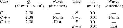
Simulations.

The naming convention in the above table is as follows:
 $C$
denotes simulations with surface cooling;
 $N,E$
denote simulations driven by down-filament/across-filament winds; and lower case
 $e,n$
denote the direction of the surface waves across-filament, down-filament, respectively.
To identify the simulations in the narrative, we borrow the nomenclature from SM18, and tag the simulations based on the surface forcing and orientation of the wave field. The nomenclature used in the narrative refers to imposed winds and waves oriented parallel to the filament axis as ‘down-filament’ while winds and waves oriented perpendicular to the filament axis as ‘across-filament’. The simulations discussed are listed in table 1 and use the shorthand naming convention: across-filament winds
 $E$
, across-filament winds plus waves
 $E+e$
; down-filament winds
 $N$
, down-filament winds plus waves
 $N+n$
; and cooling
 $C$
, cooling plus across-filament waves
 $C+e$
, cooling plus down-filament waves
 $C+n$
. All simulations use the same initial dense filament structure. In simulations with wave effects, we follow the SM18 initialization recipe and first generate restart volumes with fully developed horizontally homogeneous Langmuir turbulence. The time integration for each pre-front simulation is carried forward for approximately 25 hours to reach an equilibrium state. We prefer to use fully developed turbulence as the initial condition for the frontal calculations. Turbulence appears to stabilize the baroclinic instabilities which tend to induce large-scale meandering and long time disintegration of the density filament (e.g. Skyllingstad & Samelson Reference Skyllingstad and Samelson2012; Hamlington et al.
Reference Hamlington, Van Roekel, Fox-Kemper, Julien and Chini2014); also our initialization approach results in a finite time CFF life cycle on a time scale of order 10 to 20 hours (also see Pham & Sarkar Reference Pham and Sarkar2018); finally, the initialization recipe allows a direct comparison with our prior work. We note that Kaminski & Smyth (Reference Kaminski and Smyth2019) report that the level of background turbulence appears to impact mixed layer instabilities, for example they find energetic turbulence can modify and quench Kelvin–Helmholtz instabilities.
4 Averaging and low-order moment equations
The imposed submesoscale density filament is assumed to be two-dimensional, spatial variation in
 $(x,z)$
, and thus the LES set-up has a single homogeneous spatial direction, i.e. the down-filament or
 $y$
direction. To diagnose mean and turbulence fields we follow the recipe outlined in SM18. At any time step, a mean quantity is defined as a projection onto an
 $x$
–
 $z$
plane obtained by spatial averaging in the
 $y$
direction; this operator is indicated by
 $\langle \;\rangle$
with deviations (or fluctuations) from the average denoted by
 $(\;)^{\prime }$
. Thus, in our analysis any variable
 $f(\boldsymbol{x},t)$
is decomposed as
 $$\begin{eqnarray}f(\boldsymbol{x},t)=\langle f(x,z,t)\rangle +f^{\prime }(\boldsymbol{x},t).\end{eqnarray}$$
Practically, a down-filament average is computed from
 $\langle f\rangle =\int _{y}f\,\text{d}y/L_{y}$
, and is subject to larger random errors than the horizontal
 $x$
–
 $y$
average typically used in homogeneous LES. The archived 3-D LES volumes are large and awkward to manipulate and thus down-filament averages and statistics are computed on the fly during a simulation and stored for later use.
4.1 Average equations with surface waves
We repeat the steps in SM18 to develop an equation set for mean moments with mean turbulence correlations including wave effects. Application of
 $y$
averaging to (2.1a
) and (2.1b
), decomposing the flow fields according to the prescription (4.1) and invoking the
 $y$
averaging rules leads to the down-filament average equations
 $$\begin{eqnarray}\displaystyle \frac{\unicode[STIX]{x2202}}{\unicode[STIX]{x2202}t}\langle u\rangle & = & \displaystyle -\frac{\unicode[STIX]{x2202}}{\unicode[STIX]{x2202}x}(\langle u\rangle \langle u\rangle +\langle \unicode[STIX]{x03C0}\rangle +\langle u^{\prime }u^{\prime }+\unicode[STIX]{x1D70F}_{11}\rangle )\nonumber\\ \displaystyle & & \displaystyle -\,\frac{\unicode[STIX]{x2202}}{\unicode[STIX]{x2202}z}(\langle u\rangle \langle w\rangle +\langle u^{\prime }w^{\prime }+\unicode[STIX]{x1D70F}_{13}\rangle )+fv^{L}+v^{s}\langle \unicode[STIX]{x1D701}\rangle ,\end{eqnarray}$$
 $$\begin{eqnarray}\displaystyle \frac{\unicode[STIX]{x2202}}{\unicode[STIX]{x2202}t}\langle v\rangle & = & \displaystyle -\frac{\unicode[STIX]{x2202}}{\unicode[STIX]{x2202}x}(\langle u\rangle \langle v\rangle +\langle u^{\prime }v^{\prime }+\unicode[STIX]{x1D70F}_{12}\rangle )\nonumber\\ \displaystyle & & \displaystyle -\,\frac{\unicode[STIX]{x2202}}{\unicode[STIX]{x2202}z}(\langle v\rangle \langle w\rangle +\langle v^{\prime }w^{\prime }+\unicode[STIX]{x1D70F}_{23}\rangle )-fu^{L}-u^{s}\langle \unicode[STIX]{x1D701}\rangle ,\end{eqnarray}$$
 $$\begin{eqnarray}\displaystyle \frac{\unicode[STIX]{x2202}}{\unicode[STIX]{x2202}t}\langle w\rangle & = & \displaystyle -\frac{\unicode[STIX]{x2202}}{\unicode[STIX]{x2202}x}(\langle u\rangle \langle w\rangle +\langle u^{\prime }w^{\prime }+\unicode[STIX]{x1D70F}_{13}\rangle )+\langle b\rangle \nonumber\\ \displaystyle & & \displaystyle -\,\frac{\unicode[STIX]{x2202}}{\unicode[STIX]{x2202}z}(\langle w\rangle \langle w\rangle +\langle \unicode[STIX]{x03C0}\rangle +\langle w^{\prime }w^{\prime }+\unicode[STIX]{x1D70F}_{33}\rangle )+u^{s}\langle \unicode[STIX]{x1D702}\rangle -v^{s}\langle \unicode[STIX]{x1D709}\rangle ,\end{eqnarray}$$
 $$\begin{eqnarray}\displaystyle \frac{\unicode[STIX]{x2202}}{\unicode[STIX]{x2202}t}\langle b\rangle & = & \displaystyle -\frac{\unicode[STIX]{x2202}}{\unicode[STIX]{x2202}x}(u^{L}\langle b\rangle +\langle u^{\prime }b^{\prime }+\unicode[STIX]{x1D70F}_{1b}\rangle )\nonumber\\ \displaystyle & & \displaystyle -\,\frac{\unicode[STIX]{x2202}}{\unicode[STIX]{x2202}z}(\langle w\rangle \langle b\rangle +\langle w^{\prime }b^{\prime }+\unicode[STIX]{x1D70F}_{3b}\rangle ),\end{eqnarray}$$
 $\langle \unicode[STIX]{x1D74E}\rangle =\langle \unicode[STIX]{x1D709},\unicode[STIX]{x1D702},\unicode[STIX]{x1D701}\rangle$
. These expressions for mean currents and buoyancy are specific to our problem posing, they are obtained by adopting a 2-D density filament varying only in
 $(x,z)$
and by further assuming a horizontally homogeneous wave field. The latter assumption is likely an imperfect approximation for real wave fields near a frontal boundary where imagery shows wave breaking, induced by wave–current interaction, can occur. Wave effects are sprinkled throughout (4.2). Similar to a wavy homogeneous boundary-layer flow, Lagrangian currents
 $\boldsymbol{u}+\boldsymbol{u}^{s}=(u^{L},v^{L})$
appear in the Stokes–Coriolis terms of (4.2a
) and (4.2b
) and in the advective flux of buoyancy (4.2d
); important wave effects also appear in the expression for the vertical velocity (4.2c
). However, the present problem differs from the homogeneous wavy boundary layer where the average currents
 $\langle u,v\rangle$
are functions of
 $z$
only. Because of spatial inhomogeneity the average currents
 $\langle \boldsymbol{u}\rangle$
and hence the average vortex forces vary with
 $(x,z)$
. In particular notice the key dependence on the surface wave direction (across-filament or down-filament) and average vorticity, vertical vorticity
 $\langle \unicode[STIX]{x1D701}\rangle$
in (4.2a
), (4.2b
) and horizontal vorticity
 $\langle \unicode[STIX]{x1D709},\unicode[STIX]{x1D702}\rangle$
in (4.2c
). The above expressions are a specific instance of the general formulas derived by McWilliams (Reference McWilliams2018) using the vortex-force representation and by Suzuki & Fox-Kemper (Reference Suzuki and Fox-Kemper2016) using their so-called Stokes-shear forces.
4.2 Turbulent thermal wind with wave effects
To guide the interpretation of the simulation results, and expose the turbulence, wave and vortex-force dependencies in (4.2), we adopt the approximate turbulent thermal wind balance introduced by Gula et al. (Reference Gula, Molemaker and McWilliams2014) and considerably developed by McWilliams et al. (Reference McWilliams, Gula, Molemaker, Renault and Shchepetkin2015) and McWilliams (Reference McWilliams2018), see also SM18. TTW is a linear quasi-steady momentum balance that combines hydrostatic, geostrophic and Ekman boundary-layer dynamics. McWilliams (Reference McWilliams2018) further advances the TTW theory to account for ageostrophic advection and wave effects on currents (WEC), and is able to find diagnostic balanced solutions when the Rossby number
 $Ro=\unicode[STIX]{x1D701}/f\sim 1$
. To derive TTW for our particular wavy boundary layer we start from the
 $y$
-averaged non-hydrostatic LES equations (4.2) and follow McWilliams (Reference McWilliams2018): neglect time tendency, ageostrophic accelerations and horizontal turbulent fluxes in (4.2a
) and (4.2b
), but retain wave–current terms. A key assumption is to adopt a hydrostatic balance based on (4.2c
) with baroclinic variations and wave effects in the form
 $$\begin{eqnarray}\frac{\unicode[STIX]{x2202}\langle \unicode[STIX]{x03C0}\rangle }{\unicode[STIX]{x2202}z}=\langle b\rangle -v^{s}\langle \unicode[STIX]{x1D709}\rangle +u^{s}\langle \unicode[STIX]{x1D702}\rangle .\end{eqnarray}$$
We remark all non-hydrostatic LES models that adopt wave-averaged equations contain the average vortex forces on the right-hand side of (4.3) as well as fluctuations in vortex forces. In homogeneous boundary layers with aligned winds and waves and simple depth varying Stokes drift the gradients
 $\langle \unicode[STIX]{x1D709},\unicode[STIX]{x1D702}\rangle =\unicode[STIX]{x2202}_{z}\langle -v,u\rangle$
are only functions of
 $z$
. Leibovich (Reference Leibovich1983, p. 402) notes the vortex forces in (4.3) then formally act as unstable density stratification. For our inhomogeneous boundary layers however, the average current gradients
 $\unicode[STIX]{x2202}_{z}\langle \boldsymbol{u}\rangle$
and
 $\unicode[STIX]{x2202}_{x}\langle \boldsymbol{u}\rangle$
can vary with
 $(x,z)$
permitting variability in hydrostatic balance even for constant wave fields. In other words, spatial variations in the vortex forces in (4.3) can potentially induce horizontal forces as in a baroclinic flow. Later we show horizontal variability in the vortex forces impacts our simulations.
Next, use (4.3) to replace the horizontal pressure gradient in (4.2a
), use
 $\unicode[STIX]{x2202}_{x}\langle \unicode[STIX]{x1D709}\rangle =-\unicode[STIX]{x2202}_{z}\langle \unicode[STIX]{x1D701}\rangle$
, integrate by parts and cancel common terms. These manipulations lead to the approximate wavy TTW balance equations
 $$\begin{eqnarray}\displaystyle f\langle v\rangle & = & \displaystyle \int _{z}\frac{\unicode[STIX]{x2202}\langle b\rangle }{\unicode[STIX]{x2202}x}\,\text{d}z+\frac{\unicode[STIX]{x2202}}{\unicode[STIX]{x2202}z}\langle u^{\prime }w^{\prime }+\unicode[STIX]{x1D70F}_{13}\rangle \nonumber\\ \displaystyle & & \displaystyle -\,fv^{s}-\int _{z}\frac{\unicode[STIX]{x2202}v^{s}}{\unicode[STIX]{x2202}z}\langle \unicode[STIX]{x1D701}\rangle \,\text{d}z+\int _{z}u^{s}\frac{\unicode[STIX]{x2202}\langle \unicode[STIX]{x1D702}\rangle }{\unicode[STIX]{x2202}x}\,\text{d}z,\end{eqnarray}$$
 $$\begin{eqnarray}\displaystyle f\langle u\rangle & = & \displaystyle -\frac{\unicode[STIX]{x2202}}{\unicode[STIX]{x2202}z}\langle v^{\prime }w^{\prime }+\unicode[STIX]{x1D70F}_{23}\rangle -fu^{s}-u^{s}\langle \unicode[STIX]{x1D701}\rangle\end{eqnarray}$$
 $V_{h}$
, composite vortex force (see discussion below).
The above expressions offer interesting physical interpretations. If we neglect the turbulence and wave terms, (4.4) reduces to classic inviscid geostrophic balance between the
 $\langle v\rangle$
current and a baroclinic pressure gradient
 $\int \unicode[STIX]{x2202}_{x}\langle b\rangle \,\text{d}z/f$
. In the upper ocean boundary layer, the inviscid balance is then disrupted by vertical divergence of (Langmuir) turbulent flux, a Stokes–Coriolis effect, and new vertical integrals of vertical and down-filament vorticity weighted by Stokes drift. The new integrals, which depend on the direction of the Stokes-drift vector
 $\boldsymbol{u}^{s}$
, are structurally similar to the baroclinic horizontal pressure gradient and can induce horizontal vortex forces, we refer to these new integrals as composite vortex forces
 $\boldsymbol{V}_{\boldsymbol{h}}$
. Equations (4.4a
), (4.4b
) are diagnostic for
 $\langle v,u\rangle$
but their right-hand sides are coupled implicitly through the turbulence and now explicitly through the vorticity. In homogeneous boundary layers, the Stokes–Coriolis terms in TTW are familiar from LES, they induce an up-wave Eulerian current, i.e. a current opposite to the direction of the imposed wave field (e.g. McWilliams et al.
Reference McWilliams, Sullivan and Moeng1997; Polton, Lewis & Belcher Reference Polton, Lewis and Belcher2005). And in the case of down-filament winds the vertical flux divergence in (4.4b
) generates Ekman transport
 $\langle u\rangle$
in the
 $x$
direction. Finally, a growing body of numerical evidence and observational data finds that the turbulent fluxes and variances (Langmuir turbulence) in (4.4) depend on the surface wave field (e.g. McWilliams et al.
Reference McWilliams, Sullivan and Moeng1997; Grant & Belcher Reference Grant and Belcher2009; Kukulka et al.
Reference Kukulka, Plueddemann, Trowbridge and Sullivan2009; Sullivan & McWilliams Reference Sullivan and McWilliams2010; D’Asaro et al.
Reference D’Asaro, Thomson, Shcherbina, Harcourt, Cronin, Hemer and Fox-Kemper2014).
The spatial structure of the average vorticity in (4.4) and its orientation relative to the wave field is anticipated to be important. For example, previously we found vortex forces acting on anisotropic vorticity generated by breaking waves catalyses coherent down-welling jets overlying Langmuir turbulence (Sullivan, McWilliams & Melville Reference Sullivan, McWilliams and Melville2007a ; Sullivan et al. Reference Sullivan, McWilliams and Melville2007b ), while in a hurricane driven OBL Langmuir turbulence is enhanced or reduced by the alignment or misalignment between winds and waves (Sullivan et al. Reference Sullivan, Romero, McWilliams and Melville2012).
The horizontal vector of composite vortex forces
 $$\begin{eqnarray}\displaystyle \boldsymbol{V}_{\boldsymbol{h}}=\left(-\int _{z}\frac{\unicode[STIX]{x2202}v^{s}}{\unicode[STIX]{x2202}z}\langle \unicode[STIX]{x1D701}\rangle \,\text{d}z+\int _{z}u^{s}\frac{\unicode[STIX]{x2202}\langle \unicode[STIX]{x1D702}\rangle }{\unicode[STIX]{x2202}x}\,\text{d}z,-u^{s}\langle \unicode[STIX]{x1D701}\rangle \right) & & \displaystyle\end{eqnarray}$$
in (4.4) depends on the vertical and down-filament vorticity and the entire spectrum of surface waves that dictate the shape of the Stokes-drift profile. For a simple down-filament monochromatic wave
 $v^{s}$
decays exponentially fast over a depth scale
 $\unicode[STIX]{x1D706}=2\unicode[STIX]{x03C0}/k$
, and thus
 $V_{h}\sim -k\int v^{s}\langle \unicode[STIX]{x1D701}\rangle \,\text{d}z$
. Then the first integral in (4.5) can be large near the water surface depending on the spatial and temporal progression of frontogenesis, i.e. the life cycle of
 $\langle \unicode[STIX]{x1D701}(x,z,t)\rangle$
. Also the down-filament vorticity
 $\langle \unicode[STIX]{x1D702}(x,z,t)\rangle$
is dominated by vertical gradients
 $\unicode[STIX]{x2202}_{z}\langle u\rangle$
which are large near the surface and at the base of the thermocline. However, because of the rapid vertical decay of Stokes drift, the vertical current gradients near the thermocline are unimportant in (4.5) except for perhaps shallow mixed layers driven by high amplitude wave fields. The vortex force and Stokes-shear force, proposed by Suzuki & Fox-Kemper (Reference Suzuki and Fox-Kemper2016) and Suzuki et al. (Reference Suzuki, Fox-Kemper, Hamlington and Roekel2016), are alternative but equivalent representations of the wave-averaged equations. The latter arises by shifting some of the WEC momentum terms from the vortex force into Stokes advection and pressure gradients, neither of which involves an integrated energy exchange between waves and currents. To derive TTW using the Stokes-shear representation for our application assume a steady linearized set of horizontal Ekman momentum equations and a hydrostatic balance including the Stokes-shear force, and retain Stokes advection in all three equations,
 $$\begin{eqnarray}\displaystyle u^{s}\unicode[STIX]{x2202}_{x}\langle u\rangle & = & \displaystyle f\langle v^{L}\rangle -\unicode[STIX]{x2202}_{x}\langle p\rangle -\unicode[STIX]{x2202}_{z}\langle u^{\prime }w^{\prime }+\unicode[STIX]{x1D70F}_{13}\rangle\end{eqnarray}$$
 $$\begin{eqnarray}\displaystyle u^{s}\unicode[STIX]{x2202}_{x}\langle v\rangle & = & \displaystyle -f\langle u^{L}\rangle -\unicode[STIX]{x2202}_{z}\langle v^{\prime }w^{\prime }+\unicode[STIX]{x1D70F}_{23}\rangle\end{eqnarray}$$
 $$\begin{eqnarray}\displaystyle u^{s}\unicode[STIX]{x2202}_{x}\langle w\rangle & = & \displaystyle -\unicode[STIX]{x2202}_{z}\langle p\rangle +\langle b\rangle -\langle v^{L}\rangle \unicode[STIX]{x2202}_{z}v^{s}-\langle u^{L}\rangle \unicode[STIX]{x2202}_{z}u^{s}.\end{eqnarray}$$
 $\boldsymbol{V}_{\boldsymbol{h}}$
is then common to both representations.
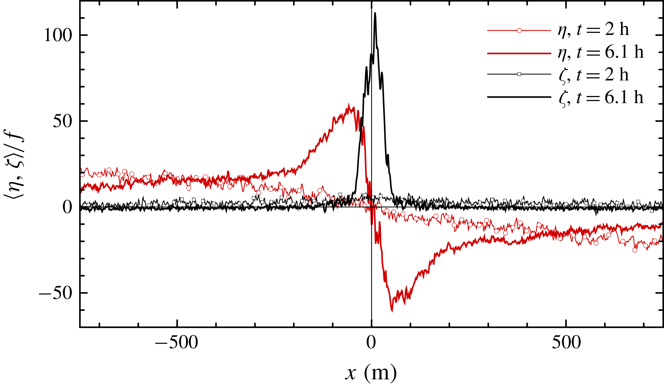
Across-filament variation of down-filament and vertical vorticities
 $\langle \unicode[STIX]{x1D702},\unicode[STIX]{x1D701}\rangle /f$
for simulation
 $C$
centred on the interval
 $x=[-750,750]~\text{m}$
near the water surface. At
 $t=2~\text{h}$
,
 $(\unicode[STIX]{x1D702},\unicode[STIX]{x1D701})$
are indicated by red/black lines with bullets, respectively, while at
 $t=6.1~\text{h},(\unicode[STIX]{x1D702},\unicode[STIX]{x1D701})$
are denoted by red and black solid lines.

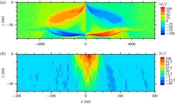
Contours of normalized average down-filament and vertical vorticities in (a) and (b) at time of peak vertical vorticity
 $t=6.1~\text{h}$
for simulation
 $C$
, see also figure 1. Notice the ranges of the horizontal and vertical axes change between the images.

To illustrate the spatial variability and amplitude of the average vorticity fields in (4.5) during idealized frontogenesis (no winds or waves) we show
 $\langle \unicode[STIX]{x1D702},\unicode[STIX]{x1D701}\rangle /f$
in figures 1 and 2 from simulation
 $C$
described in SM18. At the time of maximum frontogenesis, the amplitudes of
 $\langle \unicode[STIX]{x1D702},\unicode[STIX]{x1D701}\rangle /f$
are impressive, they approach values near 100, and near the water surface the amplitudes change rapidly over a small horizontal distance
 $\unicode[STIX]{x0394}x\sim 100~\text{m}$
. Also in this example with no surface winds
 $(\unicode[STIX]{x1D702},\unicode[STIX]{x1D701})$
are odd/even functions, respectively about the filament centreline. With down-filament waves the symmetry is broken as
 $\unicode[STIX]{x1D701}(-x)=\unicode[STIX]{x1D701}(x)>0$
tends to reinforce/oppose the baroclinic pressure gradient in (4.4a
) and hence waves potentially impact the temporal and spatial evolution of the geostrophic jets left/right of the filament centreline. Previously, McWilliams & Fox-Kemper (Reference McWilliams and Fox-Kemper2013), Suzuki & Fox-Kemper (Reference Suzuki and Fox-Kemper2016), Suzuki et al. (Reference Suzuki, Fox-Kemper, Hamlington and Roekel2016) showed how oceanic balance relations are disrupted by surface waves at low Rossby number
 $Ro<1$
. In SM18 at peak frontogenesis, the vertical vorticity is large for
 $(C,N,E)$
,
 $Ro\gg 1$
. For a fixed set of down-filament winds and waves the TTW balance (4.4a
) suggests the scaling
 $$\begin{eqnarray}\frac{V_{h}}{f\langle v\rangle }=Ro\frac{v^{s}}{\langle v\rangle }\frac{4\unicode[STIX]{x03C0}h_{i}}{\unicode[STIX]{x1D706}},\end{eqnarray}$$
and thus we anticipate surface waves to be even more important in our LES. Previously, McWilliams & Fox-Kemper (Reference McWilliams and Fox-Kemper2013) introduced the scaling in (4.7), but their analytical results only focused on
 $Ro<1$
. We note that winds and planetary rotation also break the left/right symmetry in the frontal zone even in the absence of surface waves.
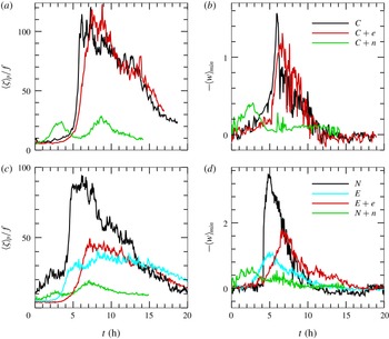
Time variation of average peak vertical vorticity
 $\langle \unicode[STIX]{x1D701}\rangle _{p}/f$
near the water surface and minimum average vertical velocity
 $\langle w\rangle _{min}$
in the middle of the OBL
 $z\sim -30~\text{m}$
at the time and spatial location of the peak vertical vorticity. Simulations driven by surface cooling and waves
 $(C,C+e,C+n)$
(a,b); simulations driven by winds and waves
 $(N+n,N,E+e,E)$
(c,d). The vertical velocity is made dimensionless by
 $(w_{\ast },u_{\ast })$
for the (cooling, wind) driven simulations, respectively.

5 Results with down-filament winds and waves
We discuss a results matrix that cuts across both wind–wave directions and varying vertical location in the boundary layer. Thus, the narrative is organized such that § 5 primarily focuses on the impact of down-filament waves while § 6 primarily focuses on the impact of across-filament waves. However, to create a compact set of figures that also allows a comparison across regimes, some plots include results for both wind–wave directions.
Past investigations of upper ocean mixing emphasize the role of down-filament winds in generating Ekman buoyancy flux (EBF) and convective instability in ocean frontogenesis, e.g. Thomas & Lee (Reference Thomas and Lee2005), Taylor & Ferrari (Reference Taylor and Ferrari2010), Thomas, Ferrari & Joyce (Reference Thomas, Ferrari and Joyce2013) and Hamlington et al. (Reference Hamlington, Van Roekel, Fox-Kemper, Julien and Chini2014). In our interpretation of filament frontogenesis, down-filament winds, as well as across-filament winds or surface cooling, are all important because the surface forcing sets the turbulent boundary-layer dynamics which is crucial in a TTW balance. For example, in idealized CFF forced by surface cooling, turbulent fluxes drive opposing secondary circulations, and these secondary circulations sharpen the across-filament current gradients which promotes further down-welling at the filament centreline (McWilliams et al. Reference McWilliams, Colas and Molemaker2009a , Reference McWilliams, Gula, Molemaker, Renault and Shchepetkin2015), and SM18. This positive feedback between turbulence, down-welling and SC leads to rapid frontogenesis. The combined action of down-filament winds, turbulence and surface waves in the life cycle of boundary-layer-induced frontogenesis is, however, largely unknown, exceptions are Suzuki & Fox-Kemper (Reference Suzuki and Fox-Kemper2016), Suzuki et al. (Reference Suzuki, Fox-Kemper, Hamlington and Roekel2016) that analyse the results from Hamlington et al. (Reference Hamlington, Van Roekel, Fox-Kemper, Julien and Chini2014). Recall that all simulations, described in § 3, are performed with fully developed wave effected turbulence at the onset of frontogenesis. To further organize the discussion of down-filament winds and waves the flow is loosely divided into a surface layer region, approximately the upper 10 m of the OBL, and the remainder of the OBL, which we call the interior region.
5.1 Surface layer
An overview of the impact of surface waves and winds on CFF is provided in figure 3. Here we show the time history of the average peak vertical vorticity
 $\langle \unicode[STIX]{x1D701}\rangle _{p}$
, computed near the surface, and the most negative value of the down-welling vertical velocity
 $-\langle w\rangle _{min}$
in the middle of the OBL as in SM18. Figure 3(a–d) compare results from simulations with and without surface waves for boundary layers forced by either surface winds or surface cooling. The results are initially unexpected and show a large impact of surface waves on the life cycle of CFF. Inclusion of down-filament surface waves significantly reduces the peak values of
 $\langle \unicode[STIX]{x1D701}\rangle _{p}$
and
 $-\langle w\rangle _{min}$
irrespective of the surface forcing. Apparently, in the present simulations down-filament surface waves alter the idealized conceptual model of filament frontogenesis (McWilliams et al.
Reference McWilliams, Gula, Molemaker, Renault and Shchepetkin2015) by disrupting the feedbacks between turbulence, down-welling and SC. A main target of the following analysis then focuses on how down-filament waves modulate CFF dynamics.
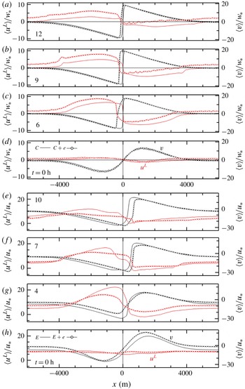
Across-filament variation of currents
 $\langle u\rangle /w_{\ast }$
(red lines, left axis) and
 $\langle v\rangle /w_{\ast }$
(black lines, right axis) for simulations driven by cooling (
 $C$
light lines) and cooling plus down-filament waves (
 $C+n$
heavy dotted lines) (a–d); simulations driven by down-filament winds (
 $N$
light lines) and down-filament winds and waves (
 $N+n$
heavy dotted lines) with normalization by
 $u_{\ast }$
(e–h).

Normalized current variances
 $\langle u^{\prime 2},v^{\prime 2},w^{\prime 2}\rangle /u_{\ast }^{2}$
(a,b,c) panels at the time of peak vertical vorticity in figure 3. Results for simulations
 $(N+n,N)$
are shown as red/green lines and
 $(E+e,E)$
are shown as cyan/black lines, respectively. In (b),
 $\langle v^{\prime 2}\rangle /u_{\ast }^{2}=59$
is the maximum value in simulation
 $E+e$
. The coloured bullets along the bottom axis mark the
 $x$
location of
 $\langle \unicode[STIX]{x1D701}\rangle _{p}/f$
for each simulation.

Down-filament 1-D energy spectra for velocity components
 $(v,u,w)$
in (a,d, b,e, c,f), respectively, at a depth
 $z\sim -10~\text{m}$
. The energy spectra are normalized by
 $u_{\ast }^{2}$
and smoothed by averaging across
 $k_{y}$
wavenumber bins and over a 100 m window centred on the
 $x$
location of the peak frontogenesis in figure 5. Results for north/east winds with and without filaments and waves are shown in panels (a–c)/(d–f), respectively. For reference we also show results from homogeneous Ekman simulations: no waves labelled
 $Ek$
and with waves labelled
 $(Ek+n,Ek+e)$
. The thin vertical line in each panel denotes the wavenumber associated with the boundary-layer depth
 $2\unicode[STIX]{x03C0}/|h_{i}|$
. Note the vertical axis is expanded in (d–f).

Running variance sum across wavenumber
 $k_{y}$
for 1-D spectra shown in figure 6, see definition (5.1). Sums for
 $\unicode[STIX]{x1D6FC}=(u,v,w)$
are indicated by red/green/blue lines, respectively, with solid lines for simulations with waves
 $(E+e,N+n)$
and dotted lines for simulations
 $(E,N)$
. The vertical dashed line in (a,b) denotes the wavenumber associated with the boundary-layer depth
 $k_{b}=2\unicode[STIX]{x03C0}/|h_{i}|$
.

Panel (a) shows across-filament variation of the average vertical vorticity
 $\langle \unicode[STIX]{x1D701}\rangle /f$
(red line), the average across-filament current
 $\langle u\rangle /u_{\ast }$
(black line) and the average down-filament Lagrangian current
 $\langle v^{L}\rangle /u_{\ast }$
(cyan line). The vorticity and currents are near the water surface
 $z\sim -5~\text{m}$
. Instantaneous down-welling velocity
 $w/u_{\ast }<0$
in a horizontal plane at
 $z=-10.5~\text{m}$
, (b). Results are for simulation
 $N+n$
with down-filament winds and waves at the time of peak vertical vorticity,
 $t=7.08~\text{h}$
. Results are shown in the far field on the west side of the front
 $x=[-4200,-2000]~\text{m}$
.

The across-filament variation of the vertical vorticity currents as in figure 8 in the frontal zone
 $x=[0,2200]~\text{m}$
.

The across-filament variation of the vertical vorticity currents as in figure 8 in the far field on the east side of the front
 $x=[3800,6000]~\text{m}$
.

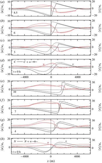
Digging deeper into the impact of down-filament waves on the life cycle of CFF, we next compare the average horizontal currents
 $\langle u,v\rangle /u_{\ast }$
at different time stamps from simulations
 $(C,C+n)$
and
 $(N,N+n)$
in figure 4. Broadly, the significant impact of down-filament waves on the evolution of CFF is independent of the surface forcing. Surface waves noticeably break the left–right odd current symmetries even in
 $C$
especially apparent right of the filament centreline
 $x>0$
. Inspection of the figures also shows down-filament waves modulate the shape and amplitude of the currents throughout the life cycle of CFF. The changes are modest at
 $t=0$
but with advancing time the shape distortions are more severe, especially in the area east of the filament centreline where we anticipate frontogenetic activity. In
 $C+n$
and
 $N+n$
the most negative/positive values of the down-filament current and the location of the maximum horizontal gradient
 $\unicode[STIX]{x2202}_{x}\langle v\rangle$
are noticeably shifted to the east compared to simulations without waves. For example, in figure 4 at
 $t=6~\text{h}$
the maximum horizontal gradients
 $\unicode[STIX]{x2202}_{x}\langle u,v\rangle$
in
 $C$
are frontogenetic, they are very sharp and tightly compacted at the filament centreline. Meanwhile in
 $C+n$
, at the same time stamp the horizontal current gradients in
 $C+n$
are greatly reduced with peak values east of the filament centreline. Closer inspection of the results in
 $(C+n,N+n)$
do show eye catching regions of weak frontogenetic activity near
 $x\sim (1000,1500)~\text{m}$
.
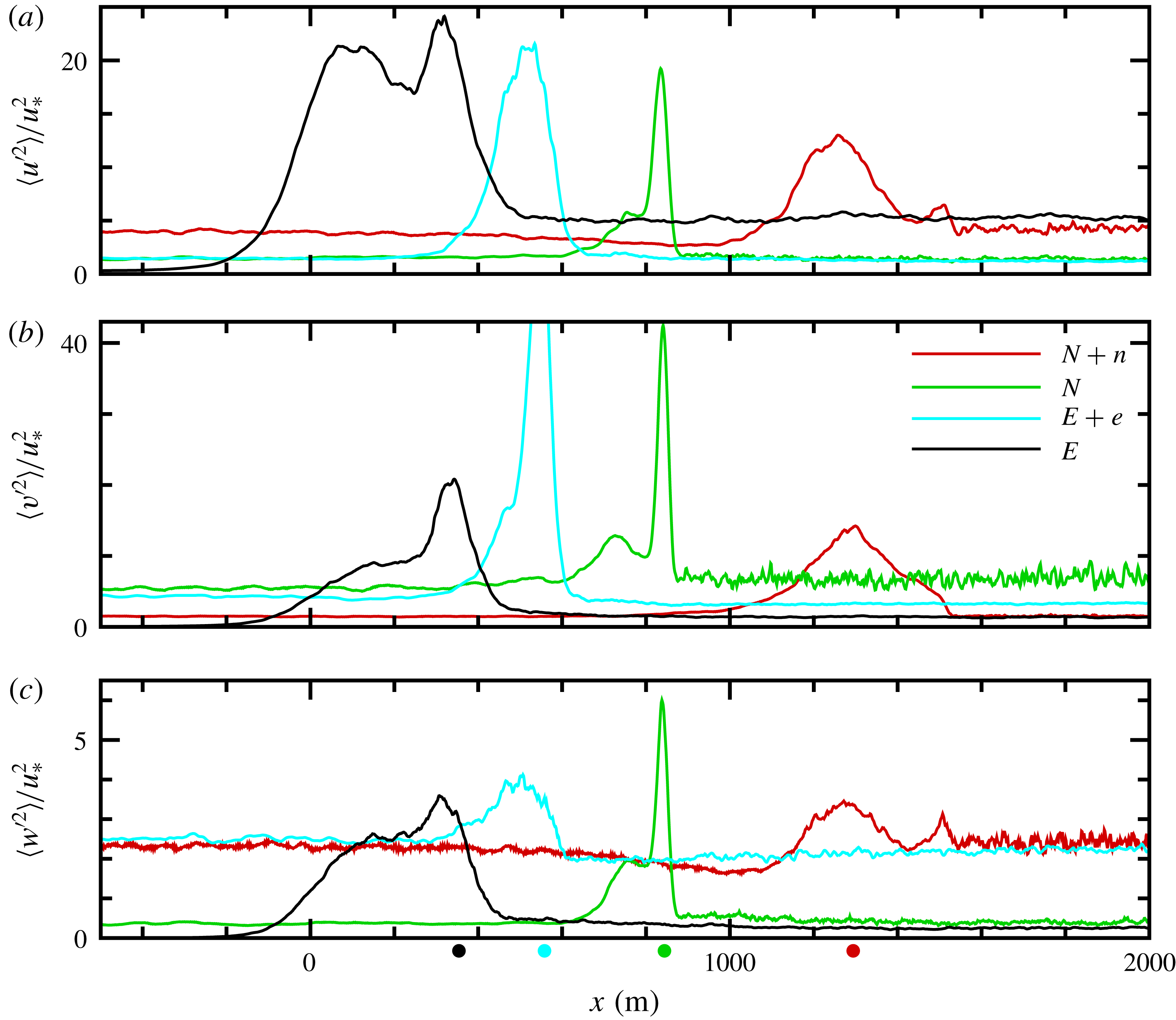
Down-filament waves also impact the turbulence statistics, and consequently the arrest mechanics in CFF as described in SM18. In figure 5, the
 $x$
variation of the resolved variances
 $\langle u^{\prime 2},v^{\prime 2},w^{\prime 2}\rangle$
are shown focusing on the frontal zone
 $x=[-500,2000]~\text{m}$
at the time of peak vertical vorticity. With down-filament winds and waves all variances are reduced compared to their counterparts obtained with down-filament winds only. Notice there are single peaks in the horizontal variances in all simulations. A key difference in
 $N+n$
compared to other simulations is the vertical velocity variance
 $\langle w^{\prime 2}\rangle$
displays two modest peaks separated by a finite distance: the maxima are located at
 $x=(1200,1500)~\text{m}$
. This hints at a complex flow in the frontal zone (see further discussion below). In simulation
 $N+n$
away from the frontal zone the horizontal variances are clearly anisotropic with
 $\langle u^{\prime 2}\rangle /u_{\ast }^{2}>\langle v^{\prime 2}\rangle /u_{\ast }^{2}$
, and the vertical variance
 $\langle w^{\prime 2}\rangle /u_{\ast }^{2}\sim 2.5$
. Similar anisotropy occurs in the far field for
 $E+e$
, but now with
 $\langle v^{\prime 2}\rangle /u_{\ast }^{2}>\langle u^{\prime 2}\rangle /u_{\ast }^{2}$
. Thus, well away from the frontal zone the magnitude of the surface layer variances in
 $(N+n,E+e)$
are consistent with spatially homogeneous boundary layers dominated by Langmuir turbulence with down-filament/across-filament waves (e.g. McWilliams et al.
Reference McWilliams, Sullivan and Moeng1997). The observed changes to the mean currents and turbulence near the filament centreline with down-filament waves are partly due to the up-wave current generated by the Stokes–Coriolis effect, but also more importantly by the horizontal composite vortex force
 $V_{h}\hat{\boldsymbol{x}}$
in (4.5).
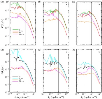
The horizontal sharpening of the buoyancy and current gradients in CFF preferentially amplifies the turbulence variances at different scales depending on the wind and wave directions. The distribution of turbulence energy across wavenumber for the
 $(u,v,w)$
velocity components is shown in figure 6. These are one-dimensional (1-D) energy spectra computed at the time of peak frontogenesis, see figure 3, and compare results for simulations with and without waves for varying surface wind direction
 $(E,E+e,N,N+n)$
. In order to fairly compare the results, all spectra are computed in the down-filament homogeneous direction, i.e. for varying down-filament wavenumber
 $k_{y}$
. Also, the spectra are smoothed by averaging across a 100 m
 $x$
-window centred on the across-filament location of the peak vertical vorticity and by averaging across
 $k_{y}$
wavenumber bins. For comparison, results from simulations of horizontally homogeneous Ekman boundary layers with and without waves are also shown; recall these homogeneous solutions serve as the restart volumes to initiate the filament simulations. The dashed vertical line in figure 6 denotes the horizontal wavenumber based on the boundary-layer depth
 $k_{b}=2\unicode[STIX]{x03C0}/|h_{i}|$
. It serves as an approximate estimate marking the transition between submesoscale and boundary-layer scales of motion.
Without waves, the variances and hence TKE are elevated across all
 $k_{y}$
under the action of CFF, in particular at low wavenumbers comparing
 $(N,E)$
with their no-wave Ekman counterparts. The enhanced low-wavenumber energy, especially in the down-filament component
 $v^{\prime }$
, is a signature of submesoscale turbulence generation by a lateral shear instability, see SM18. This low-wavenumber energy production naturally leads to a cascade of energy that elevates the
 $(u,v,w)$
variances at high wavenumbers and increased dissipation compared to the Ekman cases. Surface waves clearly change the variance partitions for
 $(u,v,w)$
especially for across-filament waves in
 $E+e$
. Meanwhile, the scale distribution of the
 $(u,v)$
variances with and without down-filament waves
 $(N,N+n)$
are surprisingly similar at a depth
 $z\sim -10~\text{m}$
. Notice, the combination of down-filament winds and waves impacts the distribution of vertical velocity energy in important ways. The amplitude of the
 $w$
spectrum at low
 $k_{y}$
is comparable in
 $(N+n,Ek+n)$
with the
 $w$
energy clearly elevated at high
 $k_{y}$
in
 $N+n$
. In other words, with down-filament winds and waves the low-frequency energy in
 $(u,v)$
is enhanced by CFF but the elevated
 $w$
energy is clearly shifted towards smaller scales compared to a homogeneous case with waves. Later, we present evidence in §§ 6.1 and 5.2 that Langmuir cells, the salient features that enhance the vertical velocity fluctuations in homogeneous simulations, are disrupted by CFF in
 $N+n$
, and also in
 $E+e$
.
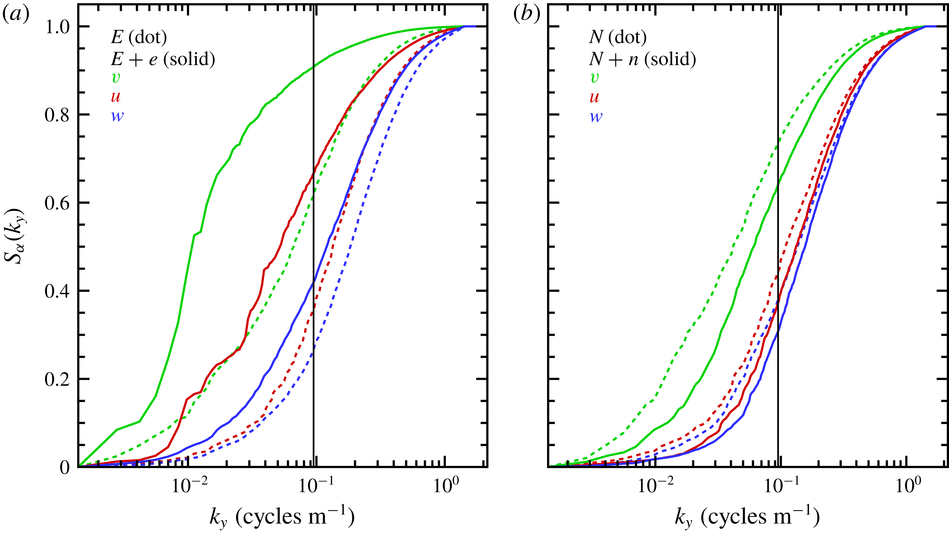
CFF enhances the spectral energy at all
 $k_{y}$
, but do surface waves alter the fractional energy balance between the submesoscale and boundary-layer regimes? To expose the energy distribution between these regimes we compute a normalized running variance (or sum)
 $$\begin{eqnarray}S_{\unicode[STIX]{x1D6FC}}(k_{y})=\int _{0}^{k_{y}}E_{\unicode[STIX]{x1D6FC}}(k_{y})\,\text{d}k_{y}/S_{\unicode[STIX]{x1D6FC}}(k_{m}),\quad \unicode[STIX]{x1D6FC}=(u,v,w)\end{eqnarray}$$
for
 $k_{y}=[0,k_{m}]$
where
 $k_{m}$
is the maximum wavenumber. Thus the sum
 $S_{\unicode[STIX]{x1D6FC}}=[0,1]$
. Results for the simulations with and without waves but including filaments are shown in figure 7. The results show most of the
 $(v,w)$
variances are supported by the submesoscale/boundary-layer regimes, respectively, with the distribution of
 $u$
variance roughly split equally between the two regimes. Surface waves in
 $E+e$
shift the energy distributions towards the submesoscale while in
 $N+n$
waves play a lesser role, but clearly induce a shift towards smaller scales compared to
 $N$
. These results add support to the hypothesis that a lateral shear instability first energizes the down-filament turbulence and that turbulence energy is subsequently redistributed to the other components with the details of the redistribution dependent on surface waves.
5.2 Langmuir patterns
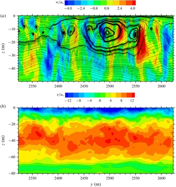
Do coherent Langmuir cells develop in filament frontogenesis with down-filament waves? The flow visualizations in figures 8–10 highlight the spatial evolution of the vertical velocity
 $w/u_{\ast }$
in an
 $x-y$
plane (depth
 $z=-10.5~\text{m}$
) at the time of peak vertical vorticity (
 $t=7.08~\text{h}$
) from simulation
 $N+n$
(the companion near-surface currents over the whole
 $x$
domain at this time are shown in figure 4
f). The images are selected sub-zones panning left-to-right across the large horizontal domain
 $(12,4.5)\times 10^{3}~\text{m}$
; the images are aspect ratio 1 to preserve the size and orientation of the turbulent structures. In each figure, the upper panel shows the corresponding
 $x$
variation of the near-surface average vertical vorticity
 $\langle \unicode[STIX]{x1D701}\rangle /f$
, across-filament current
 $\langle u\rangle /u_{\ast }$
and the down-filament Lagrangian current
 $\langle v^{L}\rangle /u_{\ast }$
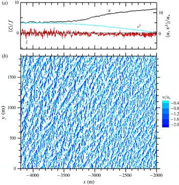
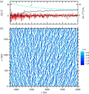
. The images reveal a web of spatially evolving turbulent Langmuir cell patterns. In the far-field (figure 10)
 $x>4000~\text{m}$
(also
 $x<-4000~\text{m}$
) the elliptical elongated patterns of down-welling are the familiar signatures of near-surface coherent Langmuir cells induced by the south–north propagating surface waves. An individual down-welling line is built from numerous forward looking Y branches along its major
 $y$
axis. On the west side of the filament axis (figure 8)
 $-4000<x<-2000~\text{m}$
the cells are less striking, the width
 $\unicode[STIX]{x1D6FF}x$
between lines appears to shrink as
 $x$
increases, and the major axis of a cell tilts eastward. These changes to the Langmuir cells appear to correlate with the growth of the secondary circulation
 $\langle u\rangle$
and down-filament (negative) jet
 $\langle v\rangle$
. Prior work (Sullivan et al.
Reference Sullivan, Romero, McWilliams and Melville2012; Van Roekel et al.
Reference Van Roekel, Fox-Kemper, Sullivan, Hamlington and Haney2012) found Langmuir cells weaken for misaligned winds and waves and here we speculate that a similar dynamics happens for misaligned waves and surface currents.
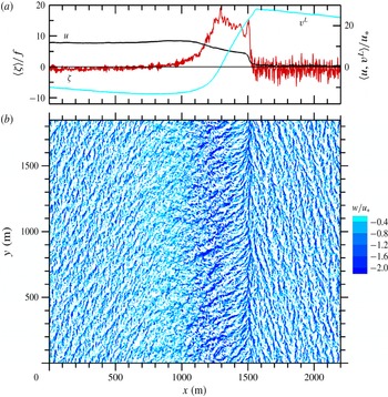
Visually, the most structure rich and dynamically complex area of the flow is the frontal zone
 $x=[0,2200]~\text{m}$
shown in figure 9. In this frontal zone, the near surface average currents and vertical vorticity
 $\langle u,v^{L},\unicode[STIX]{x1D701}\rangle$
as well as the turbulence variances (figure 5) undergo sharp changes. In figure 9, we can further identify (left, middle, right) sub-areas with distinct velocity patterns. In the left sub-area
 $0<x<1000~\text{m}$
the Langmuir cells, as identified by concentrated down-welling lines, are observed to gradually disappear with increasing
 $x$
. In this
 $x$
interval
 $\langle u,v^{L}\rangle$
are large and positive/negative compared to their far-field counterparts and the surface currents are strongly misaligned with the positive Stokes-drift velocity
 $v^{s}$
. We simply speculate this wave–current misalignment inhibits Langmuir cell development. In the right sub-area east of the frontal zone
 $x\approx 1500~\text{m}$
the visualization shows coherent Langmuir cells tilted slightly to the west. With increasing
 $x>1500~\text{m}$
, the spacing between down-welling lines widens and the lines gradually tilt northward. Overall the cell pattern east of
 $x=1500~\text{m}$
smoothly transitions into the far-field pattern shown in figure 10.
The vertical velocity patterns in the middle sub-area
 $500<x<1500~\text{m}$
highlight a complex flow transition across the frontal zone. There are large positive and negative spatial fluctuations in
 $w$
featuring organized flow patterns oriented primarily in a east or northeast direction; the patterns terminate abruptly in a south–north down-welling line near
 $x=1500~\text{m}$
. Despite their appearance, detailed animations show that the organized vertical velocity fluctuations in the region
 $1000<x<1500~\text{m}$
are not Langmuir cells originating at the water surface but are instead signatures of across-filament vortices generated by a shear instability from a large gradient
 $\unicode[STIX]{x2202}_{z}\langle v\rangle <0$
below the water surface (see §§ 5.3 and 5.4). In the frontal zone
 $1000<x<1500~\text{m}$
the vertical vorticity
 $\langle \unicode[STIX]{x1D701}\rangle$
is large and displays two modest peaks near
 $x=(1200,1500)~\text{m}$
. At the same time, the across-filament current gradient
 $\unicode[STIX]{x2202}_{x}\langle u\rangle$
is slightly negative over this region, but terminates in a much sharper negative gradient near the secondary vertical vorticity peak at
 $x=1500~\text{m}$
. Our interpretation of the flow patterns and statistics in simulation
 $N+n$
suggests that the combined action of down-filament winds and waves generates a turbulent flow that expands and weakens the concentrated narrow finite front previously found in
 $N$
. Essentially, the frontal zone in
 $N+n$
is broad and consists of two weak fronts, a primary wide front centred at
 $x=1200~\text{m}$
and a secondary narrower front located near
 $x=1500~\text{m}$
. The latter secondary front is unexpected, but extensive flow visualization at multiple time steps shows that this concentrated south–north down-welling line persists but shifts its
 $x$
location over the life cycle of CFF. Section 5.4 discusses the mechanics of how this flow feature develops with down-filament winds and waves.
The commonly accepted catalyst for generating Langmuir cells in homogeneous boundary layers with no horizontal shear is the CL2 instability mechanism pioneered by Leibovich (Reference Leibovich1983). Recently, Suzuki & Fox-Kemper (Reference Suzuki and Fox-Kemper2016) using the Stokes-shear representation of the wave-averaged equations show how to interpret the CL2 instability more broadly based on the Stokes-shear force which appears in their vertical velocity equation. For our
 $N+n$
simulation with down-filament waves the Stokes-shear force
 $S_{sf}=-v^{L}\unicode[STIX]{x2202}_{z}v^{s}=-2kv^{L}v^{s}$
, and then the predicted mechanism seeding or suppressing the CL2 instability is the sign and magnitude of the alignment between waves and currents. Inspection of figures 8–10 shows that with down-filament waves
 $v^{s}>0$
the wave–current alignment
 $\langle v^{L}\rangle v^{s}$
in
 $N+n$
varies between large negative and positive values across the domain. Viewed over the entire
 $x$
domain, see figure 4, negative wave–current alignment (suppression of CL2) is preferred for
 $t>0$
in CFF. Wave–current alignment in the far field
 $|x|>4000~\text{m}$
is well correlated with vigorous Langmuir cell patterns but is only modestly correlated with the Langmuir patterns in the frontal zone. Visualization does show smaller-scale Langmuir patterns west of the filament in the region where
 $\langle v^{L}\rangle v^{s}<0$
. In the frontal zone
 $1000<x<1500~\text{m}$
defined as the region where
 $\unicode[STIX]{x1D701}$
is large,
 $\langle v^{L}\rangle v^{s}$
switches sign near the midpoint of the interval
 $x=1290~\text{m}$
and we find minimal visual evidence of coherent Langmuir cells at
 $z=-10~\text{m}$
.
The outstanding feature of the frontal zone is the steep horizontal shear gradient
 $\unicode[STIX]{x2202}_{x}\langle v^{L}\rangle$
, i.e. large positive vertical vorticity
 $\langle \unicode[STIX]{x1D701}\rangle /f$
. In
 $N+n$
, the composite vortex force
 $V_{h}$
, which depends on the magnitude of
 $\langle \unicode[STIX]{x1D701}\rangle$
, is negative and dominates the TTW balance in the frontal zone, see § 5.3. Recall,
 $V_{h}$
is essentially the vertical integral of the average horizontal gradient of the Stokes-shear force
 $\unicode[STIX]{x2202}_{x}\langle S_{sf}\rangle$
in (4.5). Broadly, the Langmuir patterns deviate from their preferred south–north orientation in an
 $x$
interval bounded by the up-welling branches of the secondary circulation, i.e. where
 $\langle w\rangle >0$
has a local maximum in the far field on the west and east sides of filament. In this region, the flow features stable stratification, high turbulence levels and strong horizontal shear and their impact on the CL2 instability is not well understood. Li et al. (Reference Li, Zhang, Chini and Flierl2012) and Haney et al. (Reference Haney, Fox-Kemper, Julien and Webb2015) show horizontal shear complicates the mixed layer instabilities.
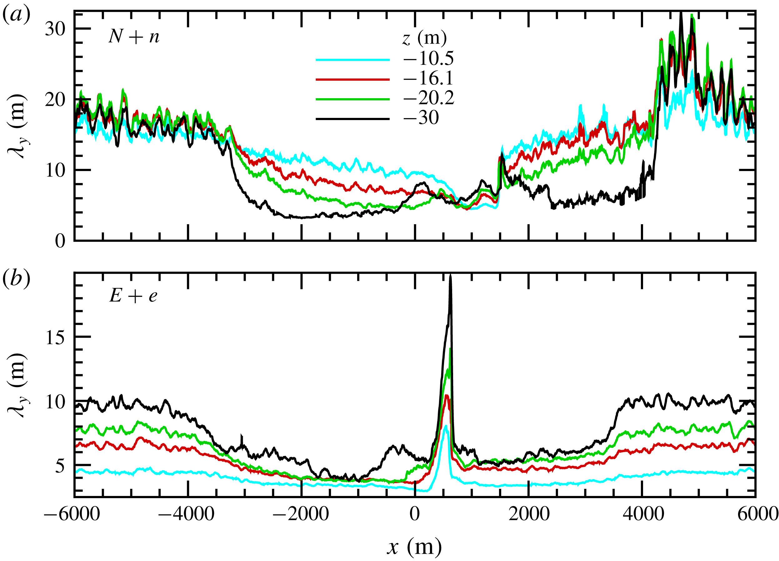
As a broad coarse measure of the horizontal scale of the vertical velocity patterns we compute the down-filament integral scale
 $$\begin{eqnarray}\unicode[STIX]{x1D706}_{y}=\int _{0}^{y0}R_{ww}({\tilde{y}})\,\text{d}{\tilde{y}},\quad \text{where }R_{ww}=\langle w^{\prime }(x,y,z)w^{\prime }(x,y+{\tilde{y}},z)\rangle /\langle w^{\prime 2}\rangle .\end{eqnarray}$$
Here
 $R_{ww}$
is the normalized autocorrelation function at particular (
 $x$
–
 $z$
) locations. The upper limit of the integral
 $y0$
is taken as the first zero crossing of
 $R_{ww}$
; the autocorrelations in (5.2) are further smoothed by averaging over a running
 $x$
window equal to 88 m. Thus in the present work,
 $\unicode[STIX]{x1D706}_{y}$
is a bulk measure of the turbulence scale in directions parallel/perpendicular to the wind, i.e. in simulation
 $(N+n,E+e)$
 $\unicode[STIX]{x1D706}_{y}$
is a rough estimate of the major/minor scale of the elliptical Langmuir cell patterns. The spatial variation of
 $\unicode[STIX]{x1D706}_{y}$
for simulations
 $(N,N+n)$
is presented in figure 11, a discussion of
 $(E,E+e)$
is postponed to § 6. In the far field of simulation
 $N+n$
 $x<-4000~\text{m}$
, where the submesoscale geostrophic and ageostrophic currents are weak, the down-filament turbulence scale is
 ${\sim}20~\text{m}$
and roughly constant over the depth of the OBL. Meanwhile in the frontal zone, where visualization shows that the Langmuir cell pattern is significantly weakened under the action of misaligned waves and currents,
 $\unicode[STIX]{x1D706}_{y}$
decreases to values less than 10 m. Apparently, the frontal dynamics in
 $N+n$
inhibits Langmuir cell development deep into the OBL. At the same time, the decrease of
 $\unicode[STIX]{x1D706}_{y}$
in the frontal zone indicates that the frontal arrest with down-filament winds and waves is most likely not a consequence of a large-scale lateral shear instability
 $\unicode[STIX]{x2202}_{x}v$
which tends to grow the down-filament turbulence scale in simulation
 $N$
, see SM18. In figure 11 for
 $N+n$
 $\unicode[STIX]{x1D706}_{y}$
exhibits a somewhat abrupt decrease/increase starting at
 $x\sim (3950,-3950)~\text{m}$
, respectively. These changes are very well correlated with the up-welling branches of the secondary circulation in the far field, i.e.
 $\langle w\rangle >0$
has a local positive maximum at
 $z\sim -30~\text{m}$
near these
 $x$
locations, also see figures 14, 15 and 16 in SM18. Figure 11 shows that submesoscale currents impact Langmuir cell development over a broad range of spatial scales outside of a narrow frontal zone for both down-filament and across-filament waves. We note
 $\unicode[STIX]{x1D706}_{y}$
is a bulk measure of the turbulence scale, and more refined sampling techniques utilizing 2-point spatial correlations and linear stochastic estimation can be used to identify the 3-D structure of coherent Langmuir cells (McWilliams et al.
Reference McWilliams, Sullivan and Moeng1997; Sullivan et al.
Reference Sullivan, Romero, McWilliams and Melville2012; McWilliams et al.
Reference McWilliams, Huckle, Liang and Sullivan2014).
The across-filament variation of the down-filament integral scale
 $\unicode[STIX]{x1D706}_{y}$
for vertical velocity at the time of peak vertical vorticity for simulations
 $(N+n,E+e)$
in panels (a)/(b), respectively. Vertical locations in metres are denoted by coloured lines
 $z$
 $=$
 $-$
10.5 (cyan),
 $-$
16.1 (red),
 $-$
20.2 (green),
 $-$
30 (black).

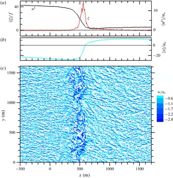
The across-filament variation of the vertical vorticity
 $\unicode[STIX]{x1D701}$
(red line) and currents
 $u$
(black line) and
 $v^{L}$
(cyan line) in (a) and (b). Instantaneous down-welling velocity
 $w/u_{\ast }<0$
, as in figure 8 in the frontal zone
 $x=[-500,1500]~\text{m}$
for simulation
 $C+n$
at the time of peak vertical vorticity
 $t=8.69~\text{h}$
. Currents are made dimensionless by
 $w_{\ast }$
.

The across-filament variation of vertical vorticity
 $\unicode[STIX]{x1D701}$
(red line), currents
 $(u,v^{L})$
(black, cyan) lines and instantaneous down-welling velocity
 $w/u_{\ast }<0$
in the far field
 $x=[2500,4200]~\text{m}$
for simulation
 $C+n$
as in figure 12.

For the LES experiments in § 3, the impact of down-filament waves on CFF is robust and generic. For example, in figure 12 we show surface flow patterns and statistics from simulation
 $C+n$
at the time of peak vertical vorticity. Remarkably, the patterns are strikingly similar to those in figure 9 despite the significant differences in surface forcing. There are two modest peaks in the vertical vorticity and the vertical velocity features two down-welling regions; a broad region for
 $x=[0,500]~\text{m}$
featuring elongated structures in a north-easterly direction, and a secondary concentrated south–north oriented line at
 $x=700~\text{m}$
. The Langmuir cells east of the secondary down-welling site are thin and very elongated. Notice also in the frontal region
 $0<x<700~\text{m}$
the zones of negative and positive wave–current alignments
 $\langle v^{L}\rangle v^{s}$
are approximately equal,
 $\langle v^{L}\rangle$
changes sign near the midpoint of this interval at
 $x\sim 340~\text{m}$
. In
 $C+n$
, the surface Langmuir number
 $La_{t}=0$
and hence the flow is in a wave dominated regime Belcher et al. (Reference Belcher, Grant, Hanley, Fox-Kemper, Van Roekel, Sullivan, Large, Brown, Hines and Calvert2012), but with background OBL turbulence generated by convection. In the far field
 $x>2500~\text{m}$
, see figure 13, the down-welling patterns gradual align in the south–north orientation and develop ‘bundles’ of Langmuir cells as described by McWilliams et al. (Reference McWilliams, Huckle, Liang and Sullivan2014) for a swell dominated regime.
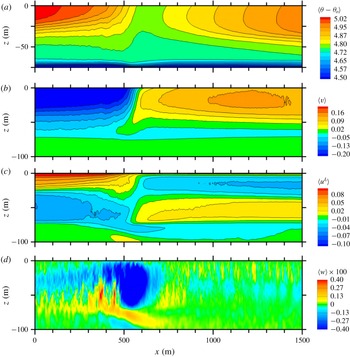
5.3 Boundary-layer interior
Average fields at
 $t=7.08~\text{h}$
for simulation
 $N+n$
. The fields displayed from (a) to (d) are temperature
 $\langle \unicode[STIX]{x1D703}-\unicode[STIX]{x1D703}_{o}\rangle$
with the colour bar in degrees K, followed by down-filament velocity
 $\langle v\rangle$
, across-filament velocity
 $\langle u\rangle$
, and vertical velocity
 $\langle w\rangle$
. Colour bars for the velocity fields are in units of
 $\text{m}~\text{s}^{-1}$
. For clarity, contour lines of
 $\langle w\rangle$
are not shown in (d).

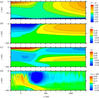
Average fields at
 $t=5.02~\text{h}$
for simulation
 $N$
. The displayed fields and labelling are the same as in figure 14 but over an
 $x$
range focused on the frontal region, also see SM18.

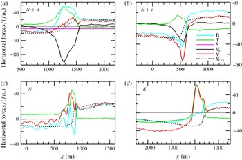
Across-filament variation of horizontal forces in the TTW balance (4.4a
) normalized by
 $fu_{\ast }$
. In addition to
 $y$
averaging the results are further averaged over the depth
 $-5.1<z<0~\text{m}$
and over a running
 $x$
window of width 60 m. The terms are as follows: B, baroclinic pressure gradient (cyan line); T, divergence of resolved turbulent flux (green line); S, Stokes–Coriolis (pink line);
 $V_{h}$
, composite vortex force (black line); V, the TTW sum (red line); and
 $V_{LES}$
, the average down-filament current computed by the LES (black dashed line). Simulations
 $(N+n,E+e)$
are (a,b) top panels and
 $(N,E)$
(c,d) bottom panels.

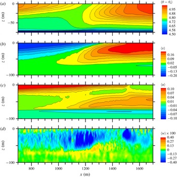
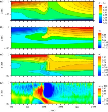
Next, we examine the impact of down-filament surface waves on the statistics and flow patterns below the water surface. Average velocity and temperature fields
 $\langle \boldsymbol{u},\unicode[STIX]{x1D703}\rangle$
from simulation
 $N+n$
in an
 $x-z$
plane at the time of peak vertical vorticity are depicted in figure 14(a–d). The horizontal extent focuses on a narrower frontal region than in figure 8,
 $x=[800,1800]~\text{m}$
. For comparison, similar fields from simulation
 $N$
(no waves) at
 $t_{m}=5.02~\text{h}$
are depicted in figure 15. Broadly, the
 $(\boldsymbol{u},\unicode[STIX]{x1D703})$
fields in
 $N+n$
exhibit more spatial complexity and, surprisingly, order-unity differences compared to their counterparts from simulation
 $N$
with down-filament winds alone, see discussion of
 $N$
in SM18. The increased complexity is induced by surface waves and in particular the coupling of average vertical vorticity and Stokes drift. Inspection of the
 $(u,v)$
panels in figure 14 shows a thin wave-effected layer near the water surface, the layer thickness is tied to the vertical decay of Stokes drift. Close inspection of the average vertical velocity
 $\langle w\rangle$
shows remnants of the instantaneous down/up welling patterns induced by Langmuir cells near the water surface;
 $y$
averaging tends to smooth out the vigorous
 $w$
fluctuations in figures 8–10. There is a conspicuous void of Langmuir cell activity in the central frontal region
 $x=[1000,1500]~\text{m}$
where we observed large amplitude
 $w$
fluctuations in figure 9. There are now two clear down-welling sites in
 $\langle w\rangle$
which are spatially well correlated with the flow visualization of
 $w$
and the double peaks in average vertical vorticity in figure 9.
To aid the interpretation of the results in figure 14, we invoke the TTW theory with wave effects outlined in § 4.2. First, notice the average negative/positive down-filament
 $v$
jets tend to overlie each other in a thin vertical layer in the frontal zone. The negative jet is tightly compressed near the water surface and expanded to the east while the positive jet is below and somewhat expanded to the west. Second, the spatial structure of
 $\langle v(x,z)\rangle$
is largely dictated by the competition between the baroclinic pressure gradient and composite vortex force in (4.4); figure 16 compares the
 $x$
variation of these two forces near the water surface. In CFF,
 $\langle \unicode[STIX]{x1D701}\rangle >0$
is a clear signature of time varying frontal sharpening, see figure 3. Thus in simulation
 $N+n$
with down-filament winds and waves
 $V_{h}$
is large, negative, even symmetric about the filament centreline and concentrated near the water surface. For the imposed wave field,
 $v^{s}$
decays to 1 % of its surface value at
 $z\sim -22~\text{m}$
. Thus,
 $V_{h}<0$
reinforces the negative baroclinic pressure gradient in the region
 $x<1000~\text{m}$
but opposes the positive baroclinic pressure gradient in the region
 $1000<x<1500~\text{m}$
near the water surface. Down-filament waves thus create amplitude asymmetry in the underlying geostrophic jets that depends on
 $\unicode[STIX]{x2202}_{z}v^{s}$
and the
 $x$
variation of
 $\unicode[STIX]{x1D701}$
. A subtle but quite important feature is the sign change in
 $V_{h}$
at
 $x=1500~\text{m}$
which also coincides with the secondary down-welling site in figure 14. Overall surface waves act as a negative feedback limiting the tendency for filament sharpening compared to
 $N$
. We emphasize this new wave effect on mean currents is separate but additive to the impact of wave-induced Langmuir turbulence on mean currents (e.g. Sullivan & McWilliams Reference Sullivan and McWilliams2010; Belcher et al.
Reference Belcher, Grant, Hanley, Fox-Kemper, Van Roekel, Sullivan, Large, Brown, Hines and Calvert2012). When viewed over the entire
 $x$
domain,
 $-6000<x<6000~\text{m}$
, wave effects do not significantly alter the large-scale patterns found in SM18 for simulation
 $N$
(not shown).
Stokes drift indirectly impacts the ageostrophic current
 $\langle u(x,z)\rangle$
, through the turbulent fluxes, and hence the secondary circulations, which are agents for frontal sharpening. In figure 14, the ageostrophic current features steep vertical gradients near the water surface which are strongly asymmetrical about the filament centreline. Previously, we found that when opposing left–right secondary circulations are disrupted filament frontogenesis is delayed, see SM18. In simulation
 $N+n$
, the ageostrophic current is generated by flux divergence
 $-\unicode[STIX]{x2202}_{z}\langle v^{\prime }w^{\prime }\rangle$
in TTW, we postpone a deeper discussion of
 $v^{\prime }w^{\prime }$
until § 5.4.
TTW is used to interpret our results, how applicable is it? Terms in the diagnostic TTW balance for the current
 $f\langle v\rangle$
, given by (4.4a
), in simulations
 $(N+n,N)$
are compared in figure 16(a,c) near the water surface. Away from the frontal zone, the TTW estimate of the geostrophic current
 $\langle v\rangle$
is dominated by the baroclinic pressure gradient B and turbulent flux divergence T and their sum is observed to be a good approximation to the average down-filament current
 $\langle v\rangle$
computed by the LES for both
 $(N+n,N)$
simulations. In the frontal zone of
 $N+n$
, the very large negative composite vortex force
 $V_{h}$
is balanced by two positive forces, the baroclinic pressure gradient B and the vertical divergence of turbulent flux T; the Stokes–Coriolis term S is small. Overall the TTW estimate of
 $\langle v\rangle$
, which neglects horizontal advection and flux divergence, remains a good approximation to its counterpart in the LES. Also, the sum
 $B+T$
is a good approximation of the LES pressure gradient
 $\unicode[STIX]{x2202}_{x}\langle p/\unicode[STIX]{x1D70C}_{o}+2e/3\rangle$
in (4.2a
) (not shown). Recall TTW assumes low Rossby number
 $Ro\sim 1$
and thus TTW is anticipated to be a better approximation in simulation
 $N+n$
, than in simulation
 $N$
where
 $\langle \unicode[STIX]{x1D701}\rangle _{p}/f\sim 100$
(see figure 3). Ageostrophic accelerations are non-negligible in
 $(C,E,N)$
. The results in figure 16 clearly show that surface wave effects are critical in frontogenesis with down-filament winds and waves.
5.4 Wave-induced vertical boundary-layer shear
Equations (4.4a
) and (4.4b
) in TTW are tightly coupled, and suggest an important role for turbulence in evolving the
 $\langle u,v\rangle$
currents. For example, the vertical divergence of turbulent flux
 $\unicode[STIX]{x2202}_{z}\langle u^{\prime }w^{\prime }\rangle$
contributes significantly to the momentum balance for the down-filament current
 $\langle v\rangle$
, as shown in figure 16. How does turbulence impact the ageostrophic current
 $\langle u\rangle$
that is central in creating secondary circulations in CFF? Sparked by (4.4b
) we next examine the generation and attributes of vertical turbulence flux
 $\langle v^{\prime }w^{\prime }\rangle$
and its impact on the ageostrophic current.
Snapshot of vertical velocity
 $w/u_{\ast }$
(colour contours) overlying instantaneous streamtraces formed from the vector
 $(v,w)/u_{\ast }$
(black lines) (a), and snapshot of down-filament current
 $v/u_{\ast }$
(b). Images are
 $y$
–
 $z$
slices from simulation
 $N+n$
at
 $t=7.08~\text{h}$
and
 $x=1200~\text{m}$
. Only a fraction of the
 $y$
domain is displayed. For spatial context see figures 9 and 14.

Vertical profiles of down-filament current
 $\langle v\rangle /u_{\ast }$
, down-filament Lagrangian current
 $\langle v+v^{s}\rangle /u_{\ast }$
and resolved vertical momentum flux
 $\langle v^{\prime }w^{\prime }\rangle /u_{\ast }^{2}$
for simulation
 $N+n$
at
 $t=7.08~\text{h}$
(a,b,c), respectively. The profiles are shown at selected
 $x$
locations in metres:
 $x$
 $=$
1007 (red), 1195 (green), 1289 (cyan), 1335 (blue), 1429 (pink), 1523 (canvas), 1945 (black),
 $\pm$
5695 (orange), for
 $x$
location context see the flow patterns in figures 9 and 14.

Figures 17(a) and 17(b) show contours of
 $(w,v)/u_{\ast }$
, respectively, but now in a down-filament
 $y$
–
 $z$
plane at the across-filament location
 $x=1200~\text{m}$
for simulation
 $N+n$
at the time of maximum vertical vorticity
 $t=7.08~\text{h}$
. The results are lightly smoothed by averaging over a 20 m
 $x$
band centred on
 $x=1200~\text{m}$
at each
 $(y,z)$
location. This
 $y$
slice through a simulation volume cuts across the intense
 $w$
fluctuations shown in figure 9 and through the average down-welling
 $\langle w\rangle$
in figure 14(d). Examination of the flow visualization illustrates important ideas: first, we observe two down-filament jets of similar amplitude but of opposite sign overlying each other; a negative jet near the surface
 $-10<z<0~\text{m}$
and a positive jet below
 $-60<z<-20~\text{m}$
. Second, the jets are fully turbulent but quasi-stationary at this time, and as a result generate a persistent and potent shear layer
 $-\unicode[STIX]{x2202}_{z}v(y,z)\gg 0$
across the entire down-filament domain at
 $z\approx -15~\text{m}$
. In hindsight, the spatial persistence of the shear layer is expected based on the pattern of the average down-filament current
 $\langle v\rangle$
in figure 14; thus in the vertical velocity equation (2.1c
) the average across-filament vorticity
 $\langle \unicode[STIX]{x1D709}\rangle =-\unicode[STIX]{x2202}_{z}\langle v\rangle >0$
near the water surface. Recall the negative and positive down-filament jets overlie each other because of the interaction between Stokes drift and vertical vorticity in (4.5). Thus, we refer to the internal shear layer that develops below the water surface as a wave-induced boundary-layer shear, a surprising new example of WEC. Based on the flow patterns in figure 14 and the vertical profiles in figure 18 the
 $z$
location of the most negative shear gradient
 $\unicode[STIX]{x2202}_{z}v<0$
approaches the water surface with increasing
 $x$
in the frontal zone
 $x=[1000,1500]~\text{m}$
; the gradient approximately disappears at
 $x=1500~\text{m}$
which also corresponds to the location where the composite vortex force changes sign, i.e.
 $V_{h}\approx 0$
in figure 16.
The amplitude of the shear gradient is particularly potent near the location of the maximum down-welling
 $x\sim 1200~\text{m}$
. The streamtraces in figure 17 illustrate that the wave-induced shear layer generates coherent structures, predominantly counterclockwise rotating vortices with their central axes roughly aligned with
 $\hat{\boldsymbol{x}}$
. In contrast, we note Langmuir cells are most often observed as pairs of clockwise and counterclockwise rotating vortices that lead to cell mergers; hence the flow structures in figure 17 are not simply Langmuir cells rotated by time and space varying winds (e.g. Sullivan et al.
Reference Sullivan, Romero, McWilliams and Melville2012; Van Roekel et al.
Reference Van Roekel, Fox-Kemper, Sullivan, Hamlington and Haney2012). The vertical shear-induced vortices generate alternating positive and negative vertical velocity fluctuations and are the source of the intense down-welling in figure 9 between
 $x=[1000,1500]~\text{m}$
. Broadly, the flow patterns in figure 17 loosely resemble those in a free shear layer (e.g. Pope Reference Pope2000, p. 139) or a stably stratified mixing layer (e.g. Werne & Fritts Reference Werne and Fritts1999; McWilliams Reference McWilliams, Federovich, Rotunno and Stevens2004). However, the flow patterns found here are unique to CFF, they are produced by steady wave forcing and develop in a spatially homogeneous direction, viz., the down-filament
 $\hat{\boldsymbol{y}}$
direction.
To connect the internal shear layer and the turbulent fluxes and mean currents we next present vertical profiles of resolved vertical flux
 $\langle v^{\prime }w^{\prime }\rangle$
and current
 $\langle v\rangle$
at selected
 $x$
locations in the frontal zone, see figure 18. First, at every
 $x$
the normalized resolved flux
 $-\langle v^{\prime }w^{\prime }\rangle /u_{\ast }^{2}\rightarrow 1$
as
 $z\rightarrow 0$
; in other words, the subgrid-scale contribution
 $\unicode[STIX]{x1D70F}_{23}$
to the total flux is confined to a very thin layer near the water surface
 $-z<2.5~\text{m}$
. Second, in the far field
 $x=\pm 5695~\text{m}$
the currents and fluxes approach values expected for homogeneous OBL Langmuir turbulence forced by down-filament winds and waves, (e.g. McWilliams et al.
Reference McWilliams, Sullivan and Moeng1997). In the far field, the
 $v$
current is uniformly mixed in the vertical and is slightly negative because of the up-wave effect caused by the Stokes–Coriolis term; the momentum flux decays monotonically with increasing depth in the OBL from its maximum value at the surface. In the frontal zone, the normalized flux tends to
 $-1$
as
 $z\rightarrow 0$
in order to match the imposed wind stress. However at fixed
 $x$
, with increasing depth the normalized flux reaches a large positive maximum below the water surface, e.g.
 $\langle v^{\prime }w^{\prime }\rangle /u_{\ast }^{2}\sim 4$
at
 $(x,z)=(1200,-20)~\text{m}$
; this location is well correlated with the position of maximum
 $-\unicode[STIX]{x2202}_{z}v$
in figure 17. Thus the large negative vertical shear in figure 17 results in a large positive flux
 $\langle v^{\prime }w^{\prime }\rangle >0$
. With increasing
 $x$
, the maximum positive flux in
 $v^{\prime }w^{\prime }$
smoothly decreases while its vertical location approaches the water surface. There is a somewhat abrupt switch in the flux variation at
 $x=1500~\text{m}$
, i.e. crossing the concentrated south–north down-welling line in figure 9. At depths below the
 $z$
location of maximum positive flux, the
 $v$
current profile reaches a maximum and then smoothly retreats and blends into the thermocline. Inspection of the vertical profiles indicates in the frontal zone the flux variation is roughly described by a simple down-gradient relationship that includes Stokes drift, i.e.
 $\langle v^{\prime }w^{\prime }\rangle \approx -K\unicode[STIX]{x2202}_{z}\langle v+v^{s}\rangle$
with
 $K$
a depth varying eddy viscosity. Proposals to refine this eddy viscosity relationship for use in larger-scale models are abundant and the topic is an intense research area, see discussion and references in McWilliams (Reference McWilliams2018, p. 494).
Vertical profiles of variances
 $\langle u^{\prime 2},v^{\prime 2},w^{\prime 2}\rangle /u_{\ast }^{2}$
(a,b,c), respectively, for the same
 $x$
locations as in figure 18.

Based on the shape of the vertical flux profiles in figure 18, the vertical divergence
 $-\unicode[STIX]{x2202}_{z}\langle v^{\prime }w^{\prime }\rangle >0$
in (4.4b
) and thus turbulence drives a concentrated positive ageostrophic current
 $\langle u\rangle$
near the water surface as shown in figure 14. With increasing
 $x$
, the vertical shear layer gradually disappears, the vertical profiles of the mean current become more uniform, the negative flux divergence abates, and hence the ageostrophic current weakens. At the termination
 $x=1500~\text{m}$
, the negative shear layer evaporates, the momentum flux profile
 $\langle v^{\prime }w^{\prime }\rangle (x,z)$
abruptly relaxes to the one-signed monotonic shape in the far field with weak vertical flux divergence and hence
 $\langle u\rangle$
drops sharply. Thus, south–north down-welling lines in figures 9 and 12 mark a transition location
 $x_{tr}$
with negative/positive vertical shear
 $\unicode[STIX]{x2202}_{z}v$
and positive/negative vertical momentum flux left/right of
 $x_{tr}$
. By continuity, a rapid decrease in
 $\unicode[STIX]{x2202}_{x}\langle u\rangle <0$
across
 $x_{tr}$
is compensated by
 $\unicode[STIX]{x2202}_{z}\langle w\rangle >0$
, i.e.
 $\langle w\rangle <0$
. Thus, wave-induced spatially varying vertical shear near the water surface is the source of the prominent south–north down-welling line in simulations with down-filament waves. The transition point
 $x_{tr}(t)$
evolves during the life cycle of CFF, but the flow features attached to the south–north down-welling line are a robust and generic feature of CFF with down-filament waves.
Vertical profiles of the resolved variances
 $\langle u^{\prime 2},v^{\prime 2},w^{\prime 2}\rangle /u_{\ast }^{2}$
in figure 19 add further support to our interpretation of the flow dynamics across the frontal zone in simulation
 $N+n$
. Outside of the frontal zone,
 $x=[1000,1500]~\text{m}$
, the shape and magnitude of the variances profiles are consistent with homogeneous Langmuir turbulence generated by down-filament winds and waves, i.e. near the surface
 $\langle u^{\prime 2}\rangle >\langle v^{\prime 2}\rangle$
and
 $\langle w^{\prime 2}\rangle /u_{\ast }^{2}\sim 3$
. In the frontal zone, because of the development of the vertical shear layer, a complicated re-ordering takes place where
 $\langle u^{\prime 2}\rangle \sim \langle v^{\prime 2}\rangle$
, and
 $\langle w^{\prime 2}\rangle$
displays a large maximum near the vertical location where
 $-\unicode[STIX]{x2202}_{z}v$
is maximum, i.e. well below the water surface.
Across-filament variation of currents
 $\langle u^{L}\rangle /w_{\ast }$
(red lines, left axis) and
 $\langle v\rangle /w_{\ast }$
(black lines, right axis) for simulations driven by cooling (
 $C$
light lines) and cooling plus across-filament waves (
 $C+e$
heavy dotted lines), (a–d); simulations driven by across-filament winds (
 $E$
light lines) and across-filament winds and waves (
 $E+e$
heavy dotted lines) with normalization by
 $u_{\ast }$
, (e–h).

6 Results with across-filament winds and waves
Our discussion of the effect of across-filament waves on CFF is abbreviated as we intend to incorporate across-filament waves into a future report focused on the influence of surface wave direction on filament frontogenesis. Across-filament waves influence the CFF dynamics, but less dramatically compared to their down-filament wave counterparts. For example, inspection of figure 3 shows that with across-filament waves the peak vorticity and minimum down-welling velocity in
 $(C,C+e)$
are comparable, with the exception that the overall timing of the peak values are slightly delayed. The same statistics for
 $(E,E+e)$
show more differences, both
 $\langle \unicode[STIX]{x1D701}\rangle _{p}$
and
 $-\langle w\rangle _{min}$
are greater in
 $E+e$
compared to
 $E$
indicative of more intense frontogenesis with across-filament waves. Post peak frontogenesis
 $t>t_{p}$
, the time decay of
 $\langle \unicode[STIX]{x1D701}\rangle /f$
and
 $\langle w\rangle _{min}$
for
 $(C,C+e)$
and
 $(E,E+e)$
are comparable, suggesting that the near-surface decay dynamics is broadly similar with and without across-filament waves.
6.1 Surface layer
Figure 20 illustrates the impact of across-filament waves on the life cycle of the near-surface average currents in simulations
 $(C+e,E+e)$
compared to
 $(C,E)$
; to smooth the statistics, the currents are again averaged over a shallow depth
 $-5<z<0~\text{m}$
(see figure 4 for a comparison with down-filament waves). At a time near peak frontogenesis
 $t\sim (9,7)~\text{h}$
the currents
 $\langle u^{L},v\rangle$
in simulations
 $(C+e,E+e)$
are similar in shape and magnitude compared to their no-wave counterparts in
 $(C,E)$
. Notice there are steep horizontal gradients in the mean currents
 $\unicode[STIX]{x2202}_{x}\langle u^{L},v\rangle$
confirming vigorous frontogenesis induced by opposing secondary circulations left and right of the filament centreline. Also, with across-filament waves the mean ageostrophic current
 $\langle u\rangle$
is reduced by an up-wave Stokes–Coriolis effect
 $-fu^{s}$
across the horizontal domain and then in the far field
 $\langle u^{L}\rangle$
in
 $E+e$
is approximately equal to
 $\langle u\rangle$
in
 $E$
.
Because of near-surface coherent Langmuir cells, across-filament waves leave a marked imprint on the turbulence. Notice in figure 5 for simulation
 $E+e$
on the west side of the filament coherent Langmuir cells energize the vertical velocity,
 $\langle w^{\prime 2}\rangle /u_{\ast }^{2}\sim 3$
extending from the far field to near the left edge of the filament, i.e. in the range
 $-6000~\text{m}<x<200~\text{m}$
. Recall in homogeneous OBLs that the vertical velocity is enhanced by factor of 2 to 3 by surface waves (e.g. McWilliams et al.
Reference McWilliams, Sullivan and Moeng1997; Harcourt & D’Asaro Reference Harcourt and D’Asaro2008; D’Asaro et al.
Reference D’Asaro, Thomson, Shcherbina, Harcourt, Cronin, Hemer and Fox-Kemper2014). In simulation
 $E$
without waves, the vertical velocity variance is noticeably reduced outside of the frontal zone,
 $x<0~\text{m}$
and
 $x>500~\text{m}$
. In both simulations
 $(E,E+e)$
, relatively warm water is advected by the ageostrophic current towards the filament centreline during frontogenesis. Then the OBL on the left side of the filament is stably stratified, warm water over cool water, also see SM18. The vertical velocity is noticeably reduced by stable stratification in
 $E$
but to a lesser degree in
 $E+e$
. Previously, Kukulka, Plueddemann & Sullivan (Reference Kukulka, Plueddemann and Sullivan2013) and others report that Langmuir turbulence continues to mix the surface layer of the OBL and prevents re-stratification under nominally stably stratified conditions. The enhancement of
 $-\langle w\rangle _{min}$
in
 $E+e$
compared to
 $E$
shown in figure 3 is a consequence of more energetic Langmuir turbulence. The Langmuir turbulence generated by across-filament waves also enhances the near-surface down-filament variance (i.e. the variance in the direction perpendicular to the wave propagation direction), thus
 $\langle v^{\prime 2}\rangle$
is larger in
 $E+e$
compared to
 $E$
outside the frontal zone. In the frontal zone the spectral results in figures 6 and 7 show enhanced
 $v^{\prime 2}$
in
 $E+e$
is mostly confined to low wavenumbers, i.e. at submesoscales larger than Langmuir turbulence or the mixed layer depth.
The across-filament variation of the average vertical vorticity
 $\langle \unicode[STIX]{x1D701}\rangle /f$
, (red line) the average across-filament Lagrangian current
 $\langle u^{L}\rangle /u_{\ast }$
, (black line) and average down-filament current
 $\langle v\rangle /u_{\ast }$
(cyan line) in (a) and (b). The vorticity and currents are near the water surface
 $z\sim -5~\text{m}$
. Instantaneous down-welling velocity
 $w/u_{\ast }<0$
in a horizontal plane at
 $z=-10.5~\text{m}$
, (c). Results are for simulation
 $E+e$
with down-filament winds and waves at the time of peak vertical vorticity,
 $t=7.19~\text{h}$
. Results are shown in the frontal zone
 $x=[-500,1700]~\text{m}$
. For comparison with down-filament waves see figure 9.

Similar to
 $N+n$
, with across-filament winds and waves the Langmuir cell patterns change markedly with varying
 $x$
across the horizontal domain. In the far field of
 $E+e$
,
 $|x|>4000~\text{m}$
vertical velocity at
 $z=-10~\text{m}$
exhibits elliptical elongated down-welling patterns as in
 $N+n$
, see figure 8, but now rotated 90 degrees from north approximately aligning with the across-filament wind and wave direction. The vertical velocity down-welling patterns in the frontal zone
 $-500~\text{m}<x<1700~\text{m}$
of
 $E+e$
are displayed in figure 21. Comparing
 $w/u_{\ast }$
between figures 21 and 9 reveals differences in flow structures at the time of peak frontogenesis that depend on the wave field orientation. In the frontal zone of
 $E+e$
the incoming and outgoing down-welling lines noticeably shrink in scale compared to their far-field counterparts. The damping effect of stable stratification on
 $w$
results in weaker Langmuir patterns outside the frontal zone. In the range
 $400<x<700~\text{m}$
where
 $\langle \unicode[STIX]{x1D701}\rangle$
is large the
 $w$
fluctuations are significant and the flow patterns are mainly oriented in a south–north direction, as opposed to the west–east direction of Langmuir cells.
In
 $E+e$
,
 $\unicode[STIX]{x1D706}_{y}$
is a bulk measure of the width (or minor axis) of the elliptical Langmuir patterns. The
 $x$
and
 $z$
variation of the across-filament integral scale
 $\unicode[STIX]{x1D706}_{y}$
is depicted in figure 11(b). Visualization of vertical velocity in homogeneous boundary layers with wave effects (e.g. McWilliams et al.
Reference McWilliams, Sullivan and Moeng1997; Sullivan et al.
Reference Sullivan, Romero, McWilliams and Melville2012), finds Langmuir cells expand with depth, and thus in the far field of
 $E+e$
at a fixed
 $x$
 $\unicode[STIX]{x1D706}_{y}$
grows with decreasing
 $z$
. Further examination of figure 11 shows that
 $\unicode[STIX]{x1D706}_{y}$
collapses in a wide
 $x$
interval bounded by the up-welling branches of the secondary circulation, i.e. where
 $\langle w\rangle >0$
has a local maximum in the far field on the west and east sides of the filament, approximately at
 $x=\pm 3500~\text{m}$
. Apparently between these
 $x$
limits the misalignment between currents and the Stokes-drift direction coupled with stable stratification disrupts the CL2 mechanics that lead to Langmuir cell formation in the OBL. Notice in figure 21 there is a narrow swath
 ${\sim}100~\text{m}$
wide spanning the
 $y$
domain featuring high amplitude
 $w$
fluctuations; the fluctuations are centred on the
 $x$
location of the peak
 $\langle \unicode[STIX]{x1D701}\rangle$
. The south–north coherence of the fluctuations coincides with a sharp increase in the integral scale
 $\unicode[STIX]{x1D706}_{y}$
. Thus in the narrow frontal zone of
 $E+e$
the dominate scale is oriented in the south–north direction, and is associated with a lateral shear instability as in
 $E$
that leads to frontal arrest, see SM18.
With across-filament waves
 $u^{s}\neq 0$
, the diagnostic TTW balance equations (4.4) contain a Stokes–Coriolis term, as expected, and two additional wave terms, a consequence of the filament horizontal heterogeneity. In
 $E+e$
, Stokes drift
 $u^{s}$
appears in the composite vortex force weighted by the horizontal gradient of the down-filament vorticity in (4.4a
) and as a multiplier on the vertical vorticity in (4.4b
). The near-surface horizontal force balance in figure 16 for
 $(E,E+e)$
illustrate strengths and weaknesses in the TTW assumptions. In both simulations the peak Rossby number
 $\langle \unicode[STIX]{x1D701}\rangle /f\sim 40$
, see figure 3, and thus as expected TTW is an inaccurate diagnostic of the LES current
 $\langle v\rangle$
in the frontal zone (McWilliams Reference McWilliams2018). The TTW trend for
 $\langle v\rangle$
is roughly correct but the amplitude is too large. Also in
 $E+e$
the composite vortex force
 $V_{h}=\int u^{s}\unicode[STIX]{x2202}_{x}\langle \unicode[STIX]{x1D702}\rangle \,\text{d}z$
is large, negative and contributes to the horizontal force balance, i.e. across-filament surface waves alter CFF. However,
 $V_{h}$
in simulation
 $E+e$
is at least a factor of two smaller in magnitude compared to its counterpart in simulation
 $N+n$
because of the dependence on
 $\langle \unicode[STIX]{x1D702}\rangle$
not
 $\langle \unicode[STIX]{x1D701}\rangle$
. East of the frontal zone the baroclinic pressure gradient B and divergence of turbulent flux T are opposite in sign and primarily balance the Coriolis force
 $f\langle v\rangle$
, and then TTW is an accurate diagnostic model for the LES current. On the west side of the filament there are differences in the TTW estimates of
 $\langle v\rangle$
. Figure 5 shows surface turbulence in
 $E$
for
 $x<0$
is noticeably weaker compared to
 $E+e$
; the secondary circulation in
 $E$
advects warm water over cool water resulting in stable stratification which suppresses the turbulence. Then horizontal mean advection plays an important role in the horizontal force balance on the west side of
 $E$
. Langmuir turbulence is less impacted by stable stratification and as a result TTW is a good approximation on the west side of
 $E+e$
.
6.2 Boundary-layer interior
The flow fields and patterns in the boundary-layer interior of
 $E+e$
are qualitatively similar to those in simulation
 $E$
, but there are important quantitative differences induced by waves. An average picture of the currents
 $\langle u^{L},v,w\rangle$
and temperature
 $\langle \unicode[STIX]{x1D703}\rangle$
in an
 $x$
–
 $z$
plane for simulation
 $E+e$
at the time of peak frontogenesis is given in figure 22. For comparison, the same fields from
 $E$
, reported in SM18, are shown in figure 23; identical contour levels and colour bars are used in the figures. An overall comparison of the fields indicates frontogenesis in
 $E+e$
is greater than in
 $E$
. Each simulation has a concentrated central down-welling jet, but
 $-\langle w\rangle _{min}$
is larger in
 $E+e$
, and the flow visualization hints at remnants from near-surface Langmuir cells located away from the frontal zone. Also, the horizontal current and buoyancy gradients, especially near the surface, are tighter and span a greater depth, and the secondary circulations left and right of the frontal zone which foster boundary-layer frontogenesis, are stronger in
 $E+e$
. Notice the horizontal current on the right side of the filament is near zero, reflecting a near balance between the wind-induced current and the opposing secondary circulation. Thus advection of cool water from the filament centre towards the east side of the filament appears small. The temperature field shows enhanced mixing on the stably stratified left side of the filament resulting from vertical transport by Langmuir turbulence as noted in figure 5. Overall across-filament waves enhance boundary-layer frontogenesis by increasing the turbulence levels, and then the arrest mechanics in
 $E+e$
are by a lateral shear instability similar to the cases without waves as reported in SM18. Compared to
 $N+n$
noteworthy differences in
 $E+e$
are: a single dominant down-welling site for average vertical velocity
 $\langle w\rangle$
; the average (positive, negative) geostrophic jets
 $\langle v\rangle$
abut each other horizontally, there is no vertical overlap of the jets; and the width of the frontal zone is narrower
 ${\sim}100~\text{m}$
as opposed to the situation with down-filament winds and waves where the width of the frontal zone is
 ${\sim}500~\text{m}$
or more.
Average fields at
 $t=8.18~\text{h}$
for simulation
 $E+e$
. The fields displayed from (a) to (d) are temperature
 $\langle \unicode[STIX]{x1D703}-\unicode[STIX]{x1D703}_{o}\rangle$
with the colour bar in degrees K, followed by down-filament velocity
 $\langle v\rangle$
, across-filament Lagrangian velocity
 $\langle u^{L}\rangle$
and vertical velocity
 $\langle w\rangle$
. Colour bars for the velocity fields are in units of
 $\text{m}~\text{s}^{-1}$
. For clarity, contour lines of
 $\langle w\rangle$
are not shown in (d).

Average fields at
 $t=4.5~\text{h}$
for simulation
 $E$
from SM18. The fields displayed from (a) to (d) are temperature
 $\langle \unicode[STIX]{x1D703}-\unicode[STIX]{x1D703}_{o}\rangle$
with the colour bar in degrees K, followed by down-filament velocity
 $\langle v\rangle$
, across-filament velocity
 $\langle u\rangle$
and vertical velocity
 $\langle w\rangle$
. Colour bars for the velocity fields are in units of
 $\text{m}~\text{s}^{-1}$
. For clarity, contour lines of
 $\langle w\rangle$
are not shown in (d).

7 Summary and conclusions
Thin filaments with widths
 ${<}100~\text{m}$
are ubiquitous on the ocean surface and are now recognized as a class of coherent structure in oceanic submesoscale turbulence (McWilliams Reference McWilliams2016). Cold filaments frequently undergo frontogenesis, (i.e. intense sharpening of their horizontal buoyancy and current gradients) which produces high levels of turbulence kinetic energy in the upper ocean boundary layer (Sullivan & McWilliams Reference Sullivan and McWilliams2018). As a result, cold filament frontogenesis is a potentially important pathway for upper ocean mixing bridging the gap between large mesoscale eddies and small-scale dissipative motions (McWilliams et al.
Reference McWilliams, Colas and Molemaker2009a
,Reference McWilliams, Molemaker and Olafsdottir
b
, Reference McWilliams, Gula, Molemaker, Renault and Shchepetkin2015).
The couplings between submesoscale filaments, currents, surface gravity waves and smaller-scale boundary-layer (Langmuir) turbulence are, however, largely unknown. To expose the interactions between these processes we examine the frontogenetic life cycle of an idealized cold dense 2-D filament interacting with upper ocean Langmuir turbulence using turbulence resolving LES. The LES model is based on the incompressible wave-averaged equations (McWilliams et al.
Reference McWilliams, Sullivan and Moeng1997). The simulations utilize large horizontal domains
 $(L_{x},L_{y})=(12,4.5)~\text{km}$
, a vertical domain
 $L_{z}=-250~\text{m}$
and fine meshes with
 $6.4\cdot 10^{9}$
grid points to capture a wide range of scale interactions spanning the submesoscale range
 $O$
(km) down to the boundary-layer scale
 $O$
(1.5 m). Process studies with surface winds and surface cooling with waves oriented in across-filament (perpendicular) and down-filament (parallel) directions relative to the 2-D filament are considered. For down-filament winds and waves the underlying baroclinic jets are simultaneously ‘up-front’ and ‘down-front’ on the west and east sides of the filament. The turbulent Langmuir number
 $La_{t}=0.32$
used in the LES is typical of a wind–wave equilibrium regime.
Based on the time series of peak vertical vorticity
 $\langle \unicode[STIX]{x1D701}\rangle _{p}$
all solutions, with and without surface waves, exhibit a frontogenetic life cycle of growth, arrest and decay in finite time
 ${\sim}20~\text{h}$
. Frontogenesis is induced by secondary circulations in the boundary layer which continually sharpen the horizontal buoyancy and current gradients with frontal arrest and decay accomplished by turbulence. The CFF is found to be strongly impacted by surface waves and in particular the wave propagation direction relative to the filament axis. The surprising influence of surface waves on CFF originates in the Stokes-drift vortex forces acting at large Rossby number
 $Ro=\unicode[STIX]{x1D701}/f>1$
. In homogeneous boundary layers Stokes-drift vortex forces primarily act on turbulent fluxes, but in the present application the boundary layer is horizontally heterogeneous and then surface waves also induce mean vortex forces that modify the hydrostatic balance (see also Suzuki et al. (Reference Suzuki, Fox-Kemper, Hamlington and Roekel2016), McWilliams (Reference McWilliams2018)). To guide the interpretation of the simulations we adopt a linear quasi-steady momentum balance that includes hydrostatic, geostrophic and Ekman boundary-layer dynamics called the turbulent thermal wind (TTW) (McWilliams Reference McWilliams2018). The TTW is diagnostic and includes wave effects, viz., Stokes–Coriolis and new composite vortex forces
 $\boldsymbol{V}_{\boldsymbol{h}}$
that depend on the spatially average vorticity field
 $\langle \unicode[STIX]{x1D74E}\rangle$
and Stokes-drift velocity
 $\boldsymbol{u}^{s}$
. Composite vortex forces introduce asymmetry, are large in magnitude near the water surface, and bias the geostrophic jets underpinning filament frontogenesis;
 $\boldsymbol{V}_{\boldsymbol{h}}$
tends to re-enforce (oppose) the negative (positive) jets on the left (right) side of the filament. Analysis of the present solutions is carried out using the original Stokes-drift vortex-force representation; Suzuki et al. (Reference Suzuki, Fox-Kemper, Hamlington and Roekel2016) propose an alternative but equivalent approach using so-called Stokes-shear forces. The composite vortex force that appears in our simulations can be derived using either representation.
Down-filament surface waves are especially impactful, they severely limit the maximum vertical vorticity
 $\langle \unicode[STIX]{x1D701}\rangle /f$
associated with CFF compared to simulations without waves. The influence of down-filament waves is independent of the surface forcing, viz., boundary layers driven by surface winds or surface cooling. Down-filament waves, also modify the ageostrophic currents, weaken the turbulence levels, and spawn primary and secondary down-welling sites over a broad frontal zone of width
 ${\sim}500~\text{m}$
; without waves the frontal zone is
 ${\sim}100~\text{m}$
. At the time of peak frontogenesis, negative/positive down-filament jets
 $\langle v\rangle$
overlie each other resulting in a vigorous vertical shear layer
 $\unicode[STIX]{x2202}_{z}v$
with large vertical momentum flux
 $\langle v^{\prime }w^{\prime }\rangle$
. CFF with across-filament waves is similar to its no-wave counterpart, but Langmuir cells on the west side of the filament, away from the frontal zone, elevate the vertical velocity and continue to mix the boundary layer despite the presence of stable stratification. At the time of peak frontogenesis TTW is a good diagnostic of the force balance for the down-filament current for simulations with down-filament winds and waves. With across-filament winds and waves, TTW is less accurate because of vigorous ageostrophic accelerations as the local Rossby number
 $Ro=\langle \unicode[STIX]{x1D701}\rangle /f\sim 40$
.
The CFF impacts the turbulence and preferentially amplifies the turbulence variances at different scales depending on the wind and wave directions. Spectra of the
 $(u,v,w)$
velocity components show the variances and hence TKE are elevated across all down-filament wavenumbers
 $k_{y}$
under the action of CFF, in particular at low wavenumbers. The enhanced low-wavenumber energy, especially in the down-filament component
 $v^{\prime }$
, is a signature of submesoscale turbulence generation by a lateral shear instability. The energy production at wavenumbers in the submesoscale range cascades energy that elevates the
 $(u,v,w)$
variances at high wavenumbers and increases the dissipation compared to horizontally homogeneous boundary layers. Surface waves change the variance partitions for
 $(u,v,w)$
especially with across-filament winds and waves. Down-filament winds and waves impact the distribution of the variances in important ways. While low-frequency energy in
 $(u,v)$
is enhanced by CFF the elevated
 $w$
energy is clearly shifted towards smaller scales compared to a homogeneous case with waves.
Strikingly, the turbulent vertical velocity patterns, indicative of coherent Langmuir cells, change markedly across the horizontal domain with both across-filament and down-filament winds. In the far field coherent cells are readily found and they enhance the near surface vertical velocity variance and the horizontal variance perpendicular to the wave propagation direction. Left and right of the frontal zone the cells first begin to rotate aligning their axes with the ageostrophic current and at the same time shrink in scale. Within the frontal zone the cells largely disappear under the action of submesoscale currents and a strong horizontal shear gradient. We speculate the CL2 instability mechanism driving the formation of Langmuir cells is disrupted by misaligned wave and current fields and stable stratification, but this requires further investigation.
Across-filament waves enhance the secondary circulations and boundary-layer frontogenesis by increasing the turbulence levels especially on the west side of the filament. Then the peak vertical vorticity and the central down-welling velocity are larger. The arrest mechanics with across-filament waves are by a lateral shear instability similar to the cases without waves as reported in SM18.
In this paper and its predecessor (SM18), the intimate dynamical relationships between submesoscale frontogenesis, arrest and decay, surface boundary-layer turbulence and surface gravity waves have been demonstrated, often with rather dramatic alterations of the behaviours in isolation from each other. However, from the present perspective of only a few illustrative simulations, it seems highly likely that the phenomenological possibilities have barely been broached.
Acknowledgements
P.P.S. was supported by the Office of Naval Research (ONR) through the Physical Oceanography Program award nos. N00014-12-1-0105, N00014-17-1-2334, N00014-18-1-2599, the Scientific Discovery through Advanced Computation (SciDAC) sponsored by the Department of Energy award no. DE-SC0012605 and by the National Science Foundation through the National Center for Atmospheric Research (NCAR). J.C.M. acknowledges support from ONR grant N00014-14-1-0626. This research benefited greatly from computer resources provided by the NCAR Strategic Capability programme managed by the NCAR Computational Information Systems Laboratory http://n2t.net/ark:/85065/d7wd3xhc, the Department of Defense High Performance Computing Modernization Program, and the Department of Energy. We thank B. Fox-Kemper and the two anonymous reviewers for their constructive comments which improved the manuscript.