Introduction
The orderly spatial distribution of various types of retinal neuron is thought to be instrumental for their uniform participation in analyzing the visual scene (Masland, Reference Masland2012). Neurons of a given type typically space themselves apart, and this intercellular spacing is often cited as a criterion for classification as a unique cell type (Cook, Reference Cook, Chalupa and Finlay1998). Their dendritic fields establish a degree of coverage characteristic of each type of retinal neuron, associated with its unique functional contribution to visual processing (Reese, Reference Reese, Masland and Albright2008). Such dendritic overlap may be extensive, for example, amongst the population of cholinergic amacrine cells, by a factor of ∼30 (Keeley et al., Reference Keeley, Whitney, Raven and Reese2007), or minimal, where dendritic arbors extend only to the tips of their homotypic neighbors, for the different retinal bipolar cell types (Wässle et al., Reference Wässle, Puller, Müller and Haverkamp2009). Such a coverage of only one dendritic arbor per retinal locus, regulated by homotypic constraints on dendritic growth, permits a “tiling” of the retinal surface despite variation in cellular density, ensuring a complete yet nonredundant spatial sampling of the visual field (Lee et al., Reference Lee, Cowgill, Al-Nabulsi, Quinn, Evans and Reese2011).
Multiple retinal bipolar cell types sample from a limited number of photoreceptor cell types, yet extract different signals for transmission to retinal ganglion cells by virtue of their distinct glutamate receptors, membrane properties, and proximity of their dendritic endings to the synaptic ribbons at the photoreceptor terminal (DeVries et al., Reference DeVries, Li and Saszik2006; Saszik and DeVries, Reference Saszik and DeVries2012; Lindstrom et al., Reference Lindstrom, Ryan, Shi and DeVries2014). Each of these functional bipolar cell populations is presumed to be organized as a regular retinal mosaic (Seung and Sumbul, Reference Seung and Sumbul2014), yet there has been little direct assessment of the spatial statistics associated with bipolar cell types (Kouyama and Marshak, Reference Kouyama and Marshak1997). Here, we have examined this expectation directly, by studying the spatial distribution of two types of retinal bipolar cell in the mouse retina. We demonstrate, by direct comparison with the populations of horizontal cells and cholinergic amacrine cells, that these bipolar cell populations are organized according to a distinct set of rules evidenced in their spatial statistics: whereas the horizontal and cholinergic amacrine cell mosaics have regularity indexes (RIs) that far exceed those for random simulations of cells, the bipolar cells have RIs comparable to those generated by random simulations. Furthermore, whereas the two former cell types exhibit an “exclusion zone” surrounding each cell that is conspicuously greater than the physical size of the cell itself, and which declines as a function of increasing cellular density across the retina, those for the bipolar cells are closer to that demanded by soma size alone, and exhibit little variation with local cell density. Finally, whereas the RI and the packing factor (PF) associated with horizontal cells and cholinergic amacrine cells exhibit minimal change as a function of density across the retina, these spatial statistics exhibit an increase as a function of density in the bipolar cell mosaics. Random simulations of cells at increasing density recapitulate these spatial features of the bipolar cell mosaics, suggesting that the bipolar cells are essentially random in their spatial distribution, constrained only by the physical packing demanded by their size.
Materials and methods
Adult retinas from the C57BL/6J (B6/J hereafter) and A/J mouse strains (The Jackson Laboratories; Bar Harbor, ME) were used for the present analysis. Mice were between 7 and 12 weeks of age, and either three or four retinas from different mice were analyzed for the different cell types in each strain. All mice were heavily anesthetized with sodium pentobarbital (Euthasol; 120 mg/kg, i.p.), and then intracardially perfused with ∼3 ml of 0.9% saline followed by ∼50 ml of 4% paraformaldehyde. Retinas were dissected, prepared as wholemounts, and immunostained as described in detail elsewhere (Keeley et al., Reference Keeley, Whitney and Reese2017). Primary antibodies were used to reveal the populations of Type 2 cone bipolar cells (mouse-anti-synaptotagmin 2, Zebrafish International Resource Center ZDB-ATB-081002-25; 1:100), Type 4 cone bipolar cells (mouse-anti-calsenilin, Millipore 05-756; 1:1,000), horizontal cells (rabbit-anti-calbindin, Millipore PC253L; 1:1,000), and cholinergic amacrine cells (goat-anti-choline acetyltransferase, Millipore AB144P; 1:200). The two bipolar cell types are OFF cone bipolar cells, and were chosen because of the availability of antibodies that reliably label their populations (Keeley et al., Reference Keeley, Whitney, Madsen, St. John, Borhanian, Leong, Williams and Reese2014a). Primary antibodies were detected using secondary antibodies conjugated to various AlexaFluor dyes (Invitrogen; 1:200). The two bipolar cell types were sampled at comparable retinal loci but in separate retinas, while the horizontal and cholinergic amacrine cell types were sampled at the identical retinal loci in the same retinas.
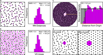
Every retina was sampled at eight retinal locations, four in the center and four in the periphery, distributed in each of the four retinal quadrants, and sample fields were 212 µm × 212 µm (for the two bipolar cell populations) or 318 µm × 318 µm (for the populations of horizontal cells and cholinergic amacrine cells of the INL) in size. Three dimensional image stacks were captured using an Olympus FluoView FV1000 scanning laser confocal microscope (Olympus, Center Valley, PA). Using ImageJ (imagej.nih.gov/ij/), the positions of every immunopositive cell in a field were marked, from which their X and Y coordinates were determined. From this two-dimensional point pattern, a variety of spatial statistics were computed for each mosaic using specialty software designed to extract the Delauney tessellation and the spatial autocorrelation of the field (Reese and Keeley, Reference Reese and Keeley2015). (Because cells positioned near the boundary of a field have ambiguous spatial statistics, these cells were excluded from each analysis. Any fields containing less than a total of 40 cells following this exclusion were eliminated, because low density fields occasionally generate spuriously high spatial statistics.) From these analyses, we derived the nearest neighbor (NN) distance (Fig. 1a) and Voronoi domain (VD) area (Fig. 1b) for each cell in the field and computed the respective RIs for each (Raven and Reese, Reference Raven and Reese2002), and constructed the density recovery profile (Fig. 1c), in turn permitting a determination of the effective radius (ER) and the PF (Fig. 1d) (Rodieck, Reference Rodieck1991). These same spatial statistics were derived from a random simulation associated to each field, in which the density of the simulated population matched each real mosaic and for which the simulated cells were assigned the mean (±s.d.) somal size derived from measurements of ten adjacent immunostained cells per field. Details of the spatial statistical analysis have recently been published (Keeley and Reese, Reference Keeley and Reese2014).
Four different spatial properties were extracted from each field of neurons. (a) The distance to the NN of each cell was measured (magenta segments) and those NN distances were plotted as a frequency distribution (shown on the right). The NNRI was calculated, being the mean divided by the standard deviation. (b) The VD area of each cell was measured (magenta tesserae), being the territory closer to each cell than to any neighboring cell, from which the VDRI was similarly calculated. (c) The spatial autocorrelation of the field was generated, being the plot of the position of all cells relative to every cell, and the density recovery profile was in turn constructed (shown on the right), from which the ER was derived. (d) The MR associated with a hexagonal matrix of identical density (shown on the right) was also derived, from which the PF of the real field was then calculated, being equal to (ER/MR)2.

Because we are only interested in comparing the regularity, spacing and packing of each cell type with its own random simulation, and are not presently concerned with either the degree of difference between the strains nor between the cell types, we have computed Student’s t-tests for these planned comparisons, using the animal averages derived from the sampled fields in each retina (usually eight fields per retina, but occasionally as few as six, when cell number in one or two fields had dropped below 40 cells). Because we are making multiple t-test comparisons (32 of them, shown in Fig. 5), we have used the Bonferroni correction to ensure a family wise error rate of P < 0.05 for determining statistical significance (indicated by an asterisk). While this increases the likelihood that we may have occasionally overlooked a real difference, it reduces the probability that any significant effect we report is itself due to chance. We have likewise used the same Bonferroni correction for determining statistical significance for the regression analysis (shown in Fig. 6), where we report the Pearson correlation coefficients computed for the variation in each of our spatial statistics as a function of increasing cellular density.
Single bipolar cell dendritic arbors were labeled as described previously (Keeley and Reese, Reference Keeley and Reese2010b). Eyes were removed from deeply anesthetized mice and immersed in 4% paraformaldehyde for 30 min. Retinas were dissected, prepared as wholemounts, and then transferred to a fixed-stage Nikon Eclipse E600 microscope (Nikon, Melville, NY). A glass micropipette with a ∼0.5 µm diameter tip was filled with a solution of the fluorescent lipophilic dye DiI (Invitrogen, V22888) and guided into the inner plexiform layer (IPL) using a micromanipulator. At the appropriate position in the IPL (see below), a small amount of DiI was deposited by passing positive current (∼100 nA) through the pipette. After making ∼50 such deposits, retinas were returned to 4% paraformaldehyde for an additional hour, and then stored in 0.1 M phosphate buffer overnight. Isolated bipolar cell somata and dendritic arbors labeled with DiI via their axon terminals were imaged the next day using an Olympus FluoView FV1000 laser scanning confocal microscope.
Four different bipolar cell types were identified using two transgenic reporter lines. Type 1A and Type 7 bipolar cells (Shekhar et al., Reference Shekhar, Lapan, Whitney, Tran, Macosko, Kowalczyk, Adiconis, Levin, Nemesh, Goldman, McCarroll, Cepko, Regev and Sanes2016) were identified as having Cyan Fluorescent Protein (CFP)-positive or Green Fluorescent Protein (GFP)-positive somata in Thy1-mitoCFP-P or GUS8.4GFP reporter mouse retinas, respectively (Wong et al., Reference Wong, Ruiz-Avila and Margolskee1999; Huang et al., Reference Huang, Max, Margolskee, Su, Masland and Euler2003; Misgeld et al., Reference Misgeld, Kerschensteiner, Bareyre, Burgess and Lichtman2007; Breuninger et al., Reference Breuninger, Puller, Haverkamp and Euler2011). These cell types were targeted by depositing DiI at the substratum of the IPL in which their axon terminals stratify. Additionally, when targeting the Type 7 bipolar cells, two types of GFP-negative cells were often labeled that could be identified as either Type 6 or Type 8 bipolar cells, based on the size and morphology of their dendritic fields (Dunn and Wong, Reference Dunn and Wong2012). A set of dye-labeled horizontal cells and cholinergic amacrine cells (i.e., starburst amacrine cells) from past studies (Reese et al., Reference Reese, Keeley, Lee and Whitney2011; Whitney et al., Reference Whitney, Keeley, St. John, Kautzman, Kay and Reese2014) were also analyzed along with these newly labeled bipolar cells. For each cell, the dendritic area was determined from a convex polygon that encompassed the entirety of the dendritic arbor. A circular profile of identical area was centered on the soma, and the proportion of the dendritic field polygon that fell outside the circular profile was determined, generating a “mismatch index”.
Results
Rationale for the spatial statistics
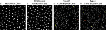
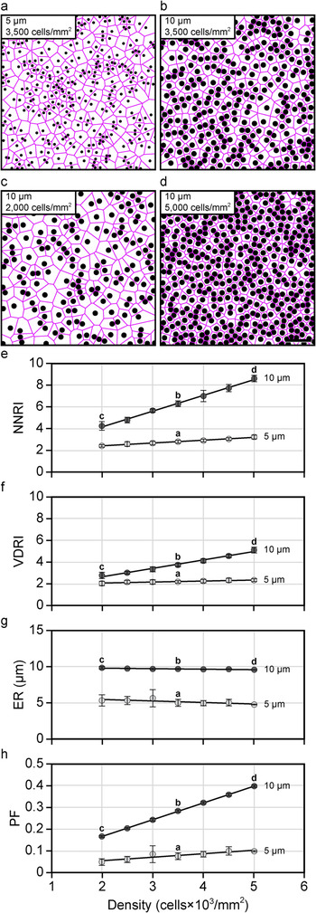
Retinal mosaics are known to vary in their degree of orderliness, but all have been shown to be more regular than a theoretical random distribution of points. By using the NN analysis to calculate the “RI” (being the mean NN distance of the cells in a field divided by the standard deviation), real mosaics consistently yield RIs well in excess of 2.0, relative to the RI of 1.91 for a Poisson point process (i.e., exhibiting complete spatial randomness). Of course, real distributions of cells within the retina are typically confined to discrete strata, wherein individual cells rarely overlie one another, and are therefore constrained in their positioning by the physical size of the cells themselves (Fig. 2). The larger the cell, the greater this constraint within a mosaic (Fig. 3a and 3b), and this constraining influence of soma size, upon the RI, must also increase as a function of cellular density (Keeley and Reese, Reference Keeley and Reese2014), for as the density increases, so the variability in potential NN distances (as well as VD areas) must decline (Fig. 3c–3f). Consequently, the degree of regularity in a mosaic is best appreciated by direct comparison with what an equally dense though random distribution of simulated cells constrained by size would achieve (Reese and Keeley, Reference Reese and Keeley2015). We have, consequently, assessed the NN regularity index (NNRI) for the populations of Type 2 and Type 4 cone bipolar cell populations, as well as for the horizontal cell and cholinergic amacrine cell populations, and compared them directly with such random (density-matched and soma-size constrained) simulations.
Retinal cell types differ in their spatial distributions. (a–d) Example fields of horizontal cells (a), cholinergic amacrine cells (b), Type 2 cone bipolar cells (c), and Type 4 cone bipolar cells (d), from B6/J retinas. Each field has been masked of all non-somal labeling, in order to emphasize the spatial patterning of each cellular population. Notice that none of the mosaics forms a precisely hexagonal lattice, yet those for the horizontal cells and cholinergic amacrine cells appear more regular in their patterning. In both of these mosaics, cells are occasionally adjacent to one another; this occurs with higher frequency, however, in the two bipolar cell mosaics. Indeed, bipolar cells of the same type occasionally appear to be compressed aside one another [e.g., yellow arrowheads in (c) and (d)], yielding an intercellular spacing that is less than the average diameter derived from measurements of their somal areas. Occasionally, bipolar cells are found isolated from nearby neighbors [e.g., orange arrows in (c) and (d)]. Calibration bar = 50 µm.

The RI and the PF must necessarily increase, for random distributions, as a function of either increasing soma size or increasing cellular density. (a and b) Simulated fields of cells at a given density (3,500 cells/mm2) but at two different sizes (5 ± 0.5 µm, and 10 ± 0.5 µm), showing how the increase in cell size reduces the variability in potential NN distances (not shown) and VD areas (magenta). (c and d) Simulated fields of cells at a given size (10.0 ± 0.5 µm) but at two different densities (2,000 and 5,000 cells/mm2), showing how the increase in cell density also reduces the variability in potential NN distances (not shown) and VD areas (magenta). (e and f) Plot of the NNRI (e) and VDRI (f) for random simulations of cells as a function of increasing cellular density at two different soma sizes, 5 ± 0.5 µm and 10 ± 0.5 µm. Both RIs increase as a function of density, but this effect is most conspicuous for the NNRI. (g and h) Plot of the ER (g) and PF (h) for random simulations of cells as a function of increasing cellular density, at these two soma sizes. The ER is determined by the space-occupying nature of randomly simulated cells, and so hardly varies as a function of cell density. Because the MR of hexagonal lattices must decline with increasing density (Fig. 1d), the PF must necessarily increase with density for random simulations of cells. For scatterplots in (e)–(h), the open circles and error bars represent the mean ± s.d. for ten random simulations. Calibration bar = 50 µm.

The NN analysis yields a RI that is based on the spatial relationship between each cell within a mosaic and its closest neighbor (Fig. 1a). Cells are, of course, not rigid circular profiles, and occasionally show the effects of crowding. As such, they may occasionally be spaced closer to one another than might be expected from the diameters derived from their somal areas (e.g., arrowheads in Fig. 2c and 2d). An alternative approach is to use VD analysis, which takes into consideration the spatial relationships between each cell and all of its immediate neighbors, by computing the territory in the plane of the mosaic closest to each cell, thereby generating the Voronoi tessellation of the field (Fig. 1b). Its advantage, in the present context, is that such occasional crowding together between cells affects the areal Voronoi domain regularity index (VDRI) statistic less severely than it does the NNRI (compare Fig. 3e with Fig. 3f). We have consequently employed this analysis as well, calculating the RI from these VD areas in a field, in order to compare these bipolar cell mosaics with their random (density-matched and soma-size constrained) simulations.
The PF is another useful spatial statistic that is acutely sensitive to variation in the density of randomly positioned cells. The PF expresses how closely a mosaic of cells approximates a regular hexagonal lattice (having a maximal value of 1.0, for perfect hexagonal packing), being dependent upon the ratio of the ER (Fig. 1c) to the maximal radius (MR; this being the intercellular distance associated with hexagonally packed elements of the same density that fill the equivalent field area, e.g., Fig. 1d) (Rodieck, Reference Rodieck1991). For randomly positioned cells, the ER is determined by soma size and generally does not vary much as a function of density (Cook, Reference Cook1996) (Fig. 3g). But when the density of randomly positioned cells steadily increases (Fig. 3b–3d), so the MR must decline accordingly, thereby increasing the PF for such random simulations (Fig. 3h). This behavior is to be contrasted with what has been described for cholinergic amacrine cells (Whitney et al., Reference Whitney, Raven, Keeley and Reese2008) and for horizontal cells (Raven et al., Reference Raven, Stagg and Reese2005a), where, despite the greater leeway for positioning at lower densities, these two cell types show either invariant or more efficient packing as density declines. The present analysis compares and contrasts these four cell types using each of the above spatial statistics, in two different strains of mice.
The spatial patterning of the mosaics
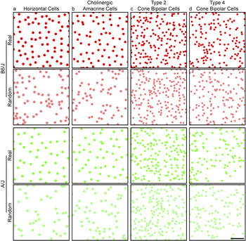
Figure 4 shows representative examples of the spatial distributions of the populations of horizontal cells and cholinergic amacrine cells, and for the Type 2 and Type 4 cone bipolar cells, from the retinas of B6/J mice (top, in red) and of A/J mice (bottom, in green). Each field is of identical area, and the elements depicting the somata are drawn to scale, adopting a size equal to the average somal area for each population, being 9.0 ± 0.8 µm (mean and s.d.) for the horizontal cells, 8.5 ± 0.5 µm for the cholinergic amacrine cells, 6.7 ± 0.5 µm for the Type 2 cone bipolar cells and 6.5 ± 0.5 µm for the Type 4 cone bipolar cells.
Plots of real cone bipolar cell mosaics appear similar to those of random distributions. (a–d) Mosaics of horizontal cells (a), cholinergic amacrine cells (b), Type 2 cone bipolar cells (c) and Type 4 cone bipolar cells (d), from B6/J (top, in red) and A/J mice (bottom, in green). Beneath each real mosaic is a simulation of a random distribution of cells matched in density and constrained by soma size (shown in desaturated color). All fields illustrated here are of the same area, and each cell portrayed in the real mosaic and in the simulation is depicted with a dot scaled to the average soma size for that cell type, to ease comparisons between the cell types. While the two strains vary in the degree of their difference in density for these four cell types, the patterning of their mosaics is comparable between the strains, yet distinct for the different cell types. Calibration bar = 50 µm.

Directly beneath each real field is a random simulation of identical density (shown in desaturated color), in which the positioning of simulated cells was constrained only by the mean (±s.d.) soma size. As we have previously reported, these different cell types differ in their average densities, with the two bipolar cell populations being denser than the horizontal cells or cholinergic amacrine cells in the mouse retina, and there are as well conspicuous strain differences in their densities, depending upon the cell type (Keeley et al., Reference Keeley, Whitney, Madsen, St. John, Borhanian, Leong, Williams and Reese2014a). Those two bipolar cell mosaics also appear less orderly by comparison with the horizontal cells and cholinergic amacrine cells (Fig. 2), but exactly how they differ, relative to the random (density-matched and soma-size constrained) simulations (Fig. 4), is not obvious without the use of spatial statistical analysis.
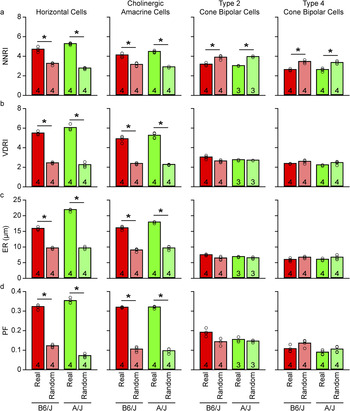
Fig. 5a plots the average NNRI for the four different cell types, presenting data derived from both the B6/J strain as well as the A/J strain. For both strains, the two cone bipolar cell types exhibit NNRIs that are well below those for the horizontal cells and cholinergic amacrine cells (Fig. 5a), as might be expected from visual inspection of their spatial distributions shown in Fig. 4. Interestingly, while the NNRIs for the mosaics of horizontal cells and cholinergic amacrine cells are conspicuously greater than those derived from random simulations matched in density and constrained by soma size, the NNRIs for the cone bipolar cell types are significantly lower than their matched random simulations (Fig. 5a). Notice too that these trends are maintained between the two different strains of mice.
The spatial properties of cone bipolar cell populations are comparable to those of random simulations. (a–d) The NNRI (a), VDRI (b), ER (c), and PF (d) for the horizontal cells, cholinergic amacrine cells, Type 2 cone bipolar cells, and Type 4 cone bipolar cells (from left to right), averaged across the individual mice (i.e., n = the number of mice, each being the average of the 6–8 fields per retina). Each pair of bars in the histogram contrasts the real data with the random (density-matched and soma-size constrained) simulations (desaturated bars), with data from B6/J on the left (red), and from A/J on the right (green). Notice that the horizontal cells and cholinergic amacrine cells are significantly different from their random (density-matched and soma-size constrained) simulations on all four spatial statistics, while the two cone bipolar cell types are significantly different only for the NNRI.

This large difference in the NNRI between the real cone bipolar cell mosaics and their random simulations is due to the fact that both Type 2 and well as Type 4 cone bipolar cell types are occasionally found closer to one another than permitted in the random simulations (e.g., Fig. 2c and 2d, yellow arrowheads), thereby increasing the variability in the range of NN distances in the real mosaics (relative to the random simulations), driving down the NNRI. This is exactly the behavior exhibited by random simulations in which soma size is reduced—the NNRI declines accordingly (Fig. 3a, 3b, and 3e). Indeed, random simulations of these cone bipolar cell populations that are given greater permission to infringe upon one another by only a couple microns (i.e., that are assigned smaller somal sizes, to simulate the reduced NN distances that are occasionally observed in these mosaics) reproduce the NNRIs observed in the real mosaics (Fig. 3e).
That the spatial ordering in these mosaics is essentially random is supported by the VD analysis of the same spatial point patterns. The RI derived from such an analysis (being the mean VD area in a field divided by the standard deviation) shows that while horizontal cells and cholinergic amacrine cells still demonstrate substantially greater VDRIs for the real mosaics relative to their random simulations, those for the two cone bipolar cell types are again substantially lower relative to the horizontal cells and cholinergic amacrine cells, but are now comparable to the VDRIs derived from their matched random simulations (Fig. 5b).
The spatial patterning present in horizontal cell mosaics and cholinergic amacrine cell mosaics has been shown to arise from the propensity for like-type cells to be spaced apart from one another: the likelihood of encountering a like-type cell is reduced in a region immediately surrounding each cell, increasing as a function of further distance from the cell, and is evidenced in the “density recovery profile” as a zone of exclusion at the origin (Fig. 1c). The size of this exclusion zone is estimated by calculating the “ER” from the density recovery profile (Rodieck, Reference Rodieck1991), and in the cases of the horizontal cells and the cholinergic amacrine cells, the ER is conspicuously larger than that obtained for random simulations matched in density and constrained by the physical size of their somata, having in the B6/J strain average ERs of 15.8 µm and 16.0 µm, respectively (Fig. 5c). For the two cone bipolar cell types, by contrast, their ERs are 7.5 µm and 6.0 µm, respectively, in the B6/J strain, comparable to that achieved by random (density-matched and soma-size constrained) simulations (Fig. 5c). The size of the ER, for these cone bipolar cell types, is, as expected, closer to their soma sizes, although the somewhat smaller ER for the Type 4 cone bipolar cells may be due to the fact that cells of this type occasionally exhibit partial overlap by being positioned at slightly variable depths in the IPL (Haverkamp et al., Reference Haverkamp, Specht, Majumdar, Zaidi, Brandstätter, Wasco, Wässle and Tom Dieck2008). This would suggest that each cone bipolar cell type is spatially constrained (relative to other homotypic cells in the mosaic) only by the physical size of the cells—beyond this, they appear to be random in their distribution. The PF analysis further supports this contention, for it shows as well that while both the horizontal cell and cholinergic amacrine cell mosaics are each packed more efficiently than their matched random simulations, the two types of cone bipolar cell mosaics achieve PFs close to those obtained by their matched random simulations (Fig. 5d).
The variation in spatial patterning as a function of density
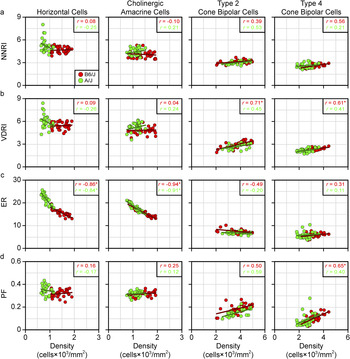
If the ER of the cone bipolar cell mosaics is determined by soma size alone, as suggested above (Fig. 5c), then it should not vary much as a function of density, as shown for the random simulations in Fig. 3g—cells can be positioned anywhere other than where another cell is positioned. Indeed, simulations have shown how robust this measure is even in the presence of conspicuous under-sampling of a mosaic (Cook, Reference Cook1996). Fig. 6c plots the variation in the ER as a function of density for each of these four populations, where striking differences in the behaviors of these mosaics is observed. Whereas the ER for the horizontal cells and cholinergic amacrine cells declines in an orderly manner as a function of increasing density, those for the two cone bipolar cell types show little variation with density. The latter is of course to be expected if only soma size regulates proximity between homotypic neighbors (Fig. 3g). That the horizontal cells and cholinergic amacrine cells show an ER substantially larger than soma size (Fig. 5c) indicates these cells must be spacing themselves apart; the fact that their ER increases as density declines (Fig. 6c) would suggest that these cells are sensing the proximity of all of their immediate neighbors as they space themselves apart.
Cone bipolar cell mosaics behave like random simulations as density varies. (a–d) Scatterplots showing the NNRI (a), VDRI (b), ER (c), and PF (d) of the real data for the four cell types (from left to right), for each individual field as a function of cellular density. The B6/J fields are shown in red while the A/J fields are shown in green. Respective regression lines are plotted, while the Pearson correlation coefficient is indicated in the top right corner, for each strain, according to color.

Such a proclivity to titrate intercellular spacing distance as a function of density may permit the maintenance of spatial patterning despite variation in the local frequency of like-type neighbors. This conclusion is borne out when considering the NNRI, the VDRI, or the PF, as a function of density (Fig. 6a, 6b and 6d), for either the horizontal cells or the cholinergic amacrine cells. Regression analysis shows little variation with increasing density, in either strain, for these cell types, evidenced by their low Pearson correlation coefficients (r), none of them being significant. By contrast, these same spatial patterning statistics, for each of the two cone bipolar cell populations, in either strain, trend toward larger values with the increase in density (note the positive correlation coefficients in Fig. 6b and 6d, for the bipolar cell types, having r values ranging from 0.4 to 0.7), although only the VDRIs for both types reached statistical significance, along with the PF for the Type 4 cone bipolar cells, and only in the B6/J strain. As indicated above, such an increase in either RI, as well as the PF, is to be expected for random simulations as they increase in density (Keeley and Reese, Reference Keeley and Reese2014), due to the reduction in the variability of potential NN distances and VD areas, or to the steady decline in the MR as the density increases (Eglen and Willshaw, Reference Eglen and Willshaw2002), respectively (Fig. 3e, 3f, and 3h). That these trends hold across different strains, discriminating two different types of cone bipolar cell from other retinal cell types known to form orderly retinal mosaics, would suggest that the general conclusion is robust: the spatial statistics of these two cone bipolar cell mosaics is clearly different from those of horizontal cells or cholinergic amacrine cells, indicating distinct biological processes responsible. The latter two cell types achieve a degree of orderliness in their patterning that is entirely absent in the cone bipolar cell types, cell types that appear to be randomly distributed across the retinal surface.
The dendritic patterning of the cells
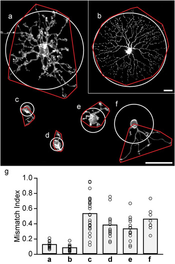
The dendritic arbors of bipolar cells in the mouse retina tile the retinal surface (Wässle et al., Reference Wässle, Puller, Müller and Haverkamp2009). If their somata exhibit such irregular spatial patterning, then their dendrites should be expected to show an irregular distribution with respect to somal positioning. We have confirmed as much in four different types of cone bipolar cells, by comparing the shape of the dendritic field (defined using a convex polygon) to a circular profile of equivalent area centered upon the soma. This irregularity in dendritic positioning was contrasted with a sample of horizontal cells and cholinergic amacrine cells that we had labeled in previous studies. Fig. 7a–7f show examples of each cell type, illustrating the spatial relationship between the dendritic field and circular profile. Both the horizontal and cholinergic amacrine cells, while not being perfectly symmetrical in their dendritic spread, have dendrites that radiate out from the soma in all directions (Fig. 7a and 7b); the bipolar cells, by contrast, have dendrites that are often conspicuously skewed to one side of the soma (Fig. 7c–7f), as should be expected if they tile the retina yet lack order in their somal patterning.
Cone bipolar cell dendritic arbors are often asymmetrically distributed relative to their somata. (a–f) Examples of a single filled horizontal cell (a), cholinergic amacrine cell (b), Type 1A cone bipolar cell (c), Type 6 cone bipolar cell (d), Type 7 cone bipolar cell (e), and Type 8 cone bipolar cell (f), illustrating the positioning of their dendritic arbors relative to their somata. Superimposed is the convex polygon enclosing the dendritic arbor (red), and a circular profile equal in area and centered upon the soma (white). (The process outside of the polygon for the horizontal cell is the axon.) (g) By expressing the area of the dendritic field lying outside the circular profile as a proportion of the total dendritic field area, a mismatch index is obtained (an index of 1.0 indicates that the entire dendritic field is offset from its predicted location centered upon the soma). The range of mismatch is substantially greater for the cone bipolar cells, to be expected from an irregular somal distribution coupled with tiling dendritic arbors. Calibration bars = 25 µm.

To quantify this observation, we measured the proportion of the dendritic field falling outside the circular profile, rendering an index of the degree of mismatch between the two territories, for 18 horizontal cells, 14 cholinergic amacrine cells, 24 Type 1A bipolar cells, 14 Type 6 bipolar cells, 14 Type 7 bipolar cells, and 8 Type 8 bipolar cells (Fig. 7g). Not every bipolar cell is skewed, as many of them show a comparably symmetrical profile as for the horizontal and cholinergic amacrine cells (Fig. 7g), but the vast majority of each type of bipolar cell lie outside the bounds defined by the other two cell types. Even those bipolar cells with low mismatch indexes should be expected: within a random distribution, some cells will undoubtedly be isolated from nearby neighbors (e.g., orange arrows in Fig. 2c and 2d) and may therefore exhibit dendritic arbors extending in all directions from the soma, approaching a more symmetrical profile. While we were unable to unambiguously label Type 2 and Type 4 bipolar cells, the most parsimonious interpretation of the present results, given the tiling behavior of all cone bipolar cell types, is that they also exhibit dendritic arbors that are comparably variable in their distribution relative to the soma.
Discussion
We have shown that the mosaics of two different types of cone bipolar cell exhibit spatial properties distinct from those of the horizontal cells and cholinergic amacrine cells. The latter cell types are organized as though they modulate their intercellular spacing to minimize proximity between like-type cells, yielding a degree of regularity in their patterning that is largely conserved across variation in density on the retina. By contrast, the mosaics of the two cone bipolar cell types have spatial properties that are reproduced by random distributions of cells, evidenced using indexes derived from tessellation-based analyses or from spatial autocorrelation analysis. From these various results, we conclude that biological processes act during development to establish the patterning of the horizontal and cholinergic amacrine cell types, yet no such processes influence each population of cone bipolar cell.
The horizontal cells and cholinergic amacrine cells have been documented to disperse tangentially during their development, and this dispersion has been suggested to reflect interactions between like-type cells that propel them apart (Galli-Resta et al., Reference Galli-Resta, Resta, Tan and Reese1997; Reese et al., Reference Reese, Necessary, Tam, Faulkner-Jones and Tan1999; Raven et al., Reference Raven, Stagg, Nassar and Reese2005b; Huckfeldt et al., Reference Huckfeldt, Schubert, Morgan, Godinho, Di Cristo, Huang and Wong2009). The two intercellular signaling proteins Multiple EGF-like-domains 10 and Multiple EGF-like-domains 11 (Megf10 and Megf11), as well as the intracellular signaling protein Pituitary tumor transforming gene 1 (Pttg1) have each been shown to play a role in the formation or maintenance of this regular intercellular spacing for these two cell types, while other cell types, like the VGluT3 amacrine cell and the Type 2 cone bipolar cell, do not require these to achieve their spatial distributions (Kay et al., Reference Kay, Chu and Sanes2012; Keeley et al., Reference Keeley, Zhou, Lu, Williams, Melmed and Reese2014b). The present analysis has examined only two of the thirteen different types of cone bipolar cell (Wässle et al., Reference Wässle, Puller, Müller and Haverkamp2009; Breuninger et al., Reference Breuninger, Puller, Haverkamp and Euler2011; Helmstaedter et al., Reference Helmstaedter, Briggman, Turaga, Jain, Seung and Denk2013; Shekhar et al., Reference Shekhar, Lapan, Whitney, Tran, Macosko, Kowalczyk, Adiconis, Levin, Nemesh, Goldman, McCarroll, Cepko, Regev and Sanes2016), and while the majority of them are comparably densely distributed in the mouse retina, whether any of the other types shows a more regular patterning in their distribution remains to be determined. A recent study in mouse retina has reported the presence of an exclusion zone for one subtype of the Type 5 cone bipolar cell, and for the Type 9 cone bipolar cell, in each case being larger than the size of the soma of these two types, but it did not report on the presence of any regularity in the patterning of their distributions (Shekhar et al., Reference Shekhar, Lapan, Whitney, Tran, Macosko, Kowalczyk, Adiconis, Levin, Nemesh, Goldman, McCarroll, Cepko, Regev and Sanes2016). While such a minimal intercellular spacing greater than soma size is characteristic of regular retinal arrays, it is not itself an index of regularity or patterning (Reese and Keeley, Reference Reese and Keeley2015), and it is interesting that the blue cone bipolar cell in the primate retina (believed to be homologous to the Type 9 cone bipolar cell in the mouse retina), while exhibiting an ER greater than soma size, has a distribution not unlike the two cone bipolar cells in the present study (Kouyama and Marshak, Reference Kouyama and Marshak1997). It will be interesting to see if the Type 5D and Type 9 cone bipolar cell populations behave like horizontal cells and cholinergic amacrine cells, scaling their exclusion zone to local density in order to maintain a comparable regularity and packing across the retina, or if they behave like the Type 2 and Type 4 bipolar cells, exhibiting an increase in PF and regularity with any increase in density. The latter result might suggest that some other passive factor, like retinal expansion, has led to a minimal spacing between cells that are otherwise randomly distributed across the retina.
Genetic variants that discriminate different strains of mice have been shown to play a role in modulating the densities of different types of retinal neurons (Keeley et al., Reference Keeley, Whitney, Madsen, St. John, Borhanian, Leong, Williams and Reese2014a). Further recent studies have shown there to be variants that modulate the patterning in their distributions independent of those modulating cell number, for the horizontal cells and cholinergic amacrine cells (Keeley and Reese, Reference Keeley and Reese2014; Keeley et al., Reference Keeley, Zhou, Lu, Williams, Melmed and Reese2014b). While the B6/J and A/J strains have only modest differences in their number of Type 2 or Type 4 cone bipolar cell types, there are still countervailing genetic variants discriminating the strains that modulate their number, shown by analysis of the panel of 26 recombinant inbred strains derived from these parental strains (Keeley et al., Reference Keeley, Whitney, Madsen, St. John, Borhanian, Leong, Williams and Reese2014a). But because the patterning in their somata largely lacks any sign of regular spacing or lattice-like packing, being essentially random in their distributions, their spatial distribution is unlikely to be governed by any active process modulated by genetic variants. We would therefore predict that an analysis of this same panel of recombinant inbred strains should show no variation in their regularity or packing beyond that predicted by their variation in density; this, however, remains to be tested.
From where such random patterning arises, during development, also remains to be determined. It may be that the factors which determine their differentiation as one type of cone bipolar cell are occurring in a stochastic, rather than precisely iterative, manner, and gene variants simply tip the set-point in that stochastic process to achieve that number. Alternatively, since both of these types of cone bipolar cell have been shown to undergo Bax-mediated cell death during development (Keeley et al., Reference Keeley, Madsen, St. John and Reese2014c), those genetic variants may simply modulate the extent of cell death eliminating a proportion of the cells that are initially produced. What is clear, from the present study, is that such programmed cell death in these two populations is not establishing any regularity to the patterning of their final mosaics (relative to random distributions), unlike, for instance, the populations of dopaminergic amacrine cells (Raven et al., Reference Raven, Eglen, Ohab and Reese2003) or of VGluT3 amacrine cells (Keeley et al., Reference Keeley, Kim, St. John and Reese2016). Finally, it remains a possibility that a more regular mosaic is originally produced, say, through periodic signals controlling their differentiation as one type or another, but that such patterning becomes perturbed as a function of further development (e.g., due to the migration and settling of later-generated cell types). This account, however, would appear to be least likely, because bipolar cells are one of the last cells to be born in the retina, and their differentiation emerges from a radial neuroblastic morphology (Morgan et al., Reference Morgan, Dhingra, Vardi and Wong2006) that would appear to anchor the cell within the radial geometry of the retinal architecture.
The different types of cone bipolar cell each tile the retina (Wässle et al., Reference Wässle, Puller, Müller and Haverkamp2009), implying a spatial precision in their sampling of the visual field, yet their somata are distributed in the least regular manner possible, short of clustering. The horizontal cells and cholinergic amacrine cells, by contrast, have conspicuously regular mosaics, yet they generate substantial dendritic overlap, producing dendritic coverage factors of ∼6 and ∼30, respectively (Reese et al., Reference Reese, Raven and Stagg2005; Keeley et al., Reference Keeley, Whitney, Raven and Reese2007). Those latter cell types produce extensive dendritic arbors within which each soma is positioned near the center of the dendritic field (Fig. 7a and 7b). The dendritic arbors of the horizontal cells are known to be sensitive to both their afferents and their homotypic neighbors, but they, along with the cholinergic amacrine cells may be programmed to generate initially symmetrical arbors around their somata that extend well into the territories of neighboring like-type cells. Indeed, the cholinergic amacrine cells show no sensitivity to the presence of their homotypic neighbors (Farajian et al., Reference Farajian, Raven, Cusato and Reese2004). Cone bipolar cells, by contrast, wind up with dendritic arbors that are conspicuously irregular in their distribution around their somata (Fig. 7c–7g), extending their dendrites during development to colonize near-exclusively each cone pedicle within their territory (Lee et al., Reference Lee, Cowgill, Al-Nabulsi, Quinn, Evans and Reese2011). Indeed, the tiled dendritic territories of the Type 2 cells are strikingly variable in their sizes (Wässle et al., Reference Wässle, Puller, Müller and Haverkamp2009), as would be predicted given the random nature of their somal distributions shown herein. Such a strategy of directed targeting and exclusive colonization, constrained by homotypic interactions to restrict overall field size, ensures a uniform sampling by tiled dendritic arbors despite the random distribution of their somata.
In sum, we have demonstrated that two populations of retinal neurons with laterally oriented and overlapping processes exhibit spatial order in their local distributions, while two other populations with radially oriented processes do not. While we believe that the present results will prove to be generalizable to all bipolar cell types, present evidence suggests that not all amacrine cell types behave like the cholinergic amacrine cells (Raven et al., Reference Raven, Eglen, Ohab and Reese2003; Keeley et al., Reference Keeley, Kim, St. John and Reese2016). To date, no exclusive markers for different retinal ganglion cell types have become available; though one might predict that those types associated with nonimage forming functions should be least likely to exhibit dendritic tiling or regularity in their somal distributions. As reviewed elsewhere, the patterning and dendritic coverage of different retinal cell types is unique to each cell type, likely tied to their unique contributions to retinal function (Reese and Keeley, Reference Reese and Keeley2015).