


Introduction
Wheat (Triticum aestivum L.) is a major cereal crop globally (Giraldo et al., Reference Giraldo, Benavente, Manzano-Agugliaro and Gimenez2019) and a key component of food security in South Asia, including Pakistan (Ali et al., Reference Ali, Ali, Ali and Waqar2013). However, wheat production is strongly influenced by drought, unpredictable weather patterns like temperature fluctuations and rainfall, and insect pest pressure particularly aphids whose population are sensitive to temperature, humidity and crop phenology (Macfadyen and Hill, Reference Macfadyen and Hill2018; Faheem et al., Reference Faheem, Saeed, Sajjad, Wang and Ali2019; Ullah et al., Reference Ullah, Abbas, Gul, Güncan, Hafeez, Gadratagi, Cicero, Ramirez-Romero, Desneux and Li2024). These tiny insects not only damage the crop by feeding on it directly but also spread viral diseases, making their impact even more harmful (Simon et al., Reference Simon, Caulfield, Hammond-Kosack, Field and Aradottir2021; Dara et al., Reference Dara, Abbas, Temitope, Li, Guohua and Wenxian2025). Under favourable environmental conditions, aphid population can grow quickly (Gong et al., Reference Gong, Chen, Wang, Li, Li, Zhang, Li and Zhu2021). When feeding is severe, it disrupts normal physiological functioning, which in turn reduces wheat yield (Singh et al., Reference Singh, Simon, Halsey, Kurup, Clark and Aradottir2020; Abbas et al., Reference Abbas, Dara, Ullah, Saddam, Abbas, Alam, Babar, Hafeez, Gogi, Ghramh and Khan2025). In Pakistan, wheat yield losses from aphids are estimated at 7.9–34.2% (Shahid et al., Reference Shahid, Zia, Naeem and Naz2012; Ali et al., Reference Ali, Zulkiffal, Anwar, Hussain, Farooq and Khan2015). Direct feeding led to 10–50% yield loss, while the indirect feeding led to 20–80% yield loss (Yahya et al., Reference Yahya, Saeed, Nadeem, Hamed and Shokat2017).
Numerous agronomic and ecological prospects influence aphid population size in wheat including time of sowing, prevailing environmental conditions, host plant genotype and biological regulation by natural enemies (Saleem et al., Reference Saleem, Ullah and Ashfaque2009; Zhang et al., Reference Zhang, Li, Quandahor, Gou, Li, Zhang, Haq, Ma and Liu2022). Among cultural practices, sowing date is particularly important because it determines the environmental conditions under which aphid population develop, rather than full seasonal phenology of aphid outbreak (Mohammed et al., Reference Mohammed, Desneux, Fan, Han, Ali, Song and Gao2018). Variation in sowing time further alters exposure to temperature, relative humidity and rainfall regimes that directly affect aphid survival and reproduction (Hameed et al., Reference Hameed, Muhammad and Shah2025).
Abiotic factors in relation with different sowing dates play a central role in shaping aphid population build-up. Moderate temperatures and higher relative humidity are known to favour aphid multiplication, whereas extreme heat or low humidity suppress population growth (Ali et al., Reference Ali, Naseem, Arshad, Ashraf, Rizwan, Tahir, Rizwan, Sayed, Ullah, Khan, Amir, Pan and Liu2021). Thus, differences in sowing time can indirectly influence aphid abundance by modifying the microclimatic conditions experienced during key infestation periods (Singh et al., Reference Singh, Simon, Halsey, Kurup, Clark and Aradottir2020).
Host plant genotype is another critical determinant of aphid population dynamics. Wheat genotypes differ in morphological and physiological traits that affect aphid colonisation, feeding efficiency, and population growth. Genotype-specific responses can therefore mediate aphid abundance under similar environmental conditions and represent an important component of sustainable pest management (Gao et al., Reference Gao, Shen, Chen, Lai, Yang, Li, Zhao and Ge2023). In addition to abiotic and host plant factors, natural enemies contribute to regulating aphid populations in wheat agroecosystems. Predators and parasitoids can suppress aphid densities, and their activity is often influenced by both environmental conditions and crop management practices, including sowing time. Although natural enemy abundance was not quantified directly, their potential regulatory role was considered as part of the broader biotic context influencing observed aphid population patterns (Snyder, Reference Snyder2019).
In light of the above, this study focuses on predicting aphid population dynamics as the response variable, using sowing date, wheat genotype, and associated abiotic and biotic factors as explanatory variables. Understanding how variation in sowing dates influences aphid population trends over time is therefore essential for developing effective and ecologically sustainable pest management strategies. This is particularly crucial for resource-limited farmers in developing countries who cannot afford extensive chemical control measures. Integrated pest management (IPM) strategies that include adjustment of sowing time can significantly reduce reliance on insecticides, lower production costs, and mitigate the environmental risks associated with pesticide use (Pretty and Bharucha, Reference Pretty and Bharucha2015).
This article aims to investigate the impact of different sowing dates on aphid population build-up in wheat fields, with a focus on identifying optimal sowing windows that minimise pest pressure while maintaining or enhancing crop productivity. The study will contribute to a better understanding of agroecological pest control and support the development of sustainable wheat production practices in aphid-prone regions.
Materials and methods
Experimental set-up and data collection
The research was conducted during the 2024 and 2025 cropping season, at the Wheat Research Institute, Faisalabad (latitude: 31.390648 and longitude: 73.041677). Twelve advanced genotypes (The material utilised in 8–9 years of selection: Akbar-19, Subhani-21, Dilkash-20, Arooj-22, V-7016S1, V-21243, V-20330, V-19317, V-21580, V-22426, V-22424 and V-22647) were evaluated. The experiment was conducted using a split-plot design. Sowing date was assigned to the main plots, while wheat genotypes were assigned to sub-plots within each sowing date. Within each block, wheat genotypes were randomised independently for every sowing date. The main plots (sowing dates) were randomised across blocks to avoid positional bias.
Each treatment combination was replicated three times, resulting in three blocks per sowing date, with all genotypes represented once within each block. This design ensured adequate replication and proper randomisation for evaluating the effects of sowing date, genotype, and their associated environmental influences on aphid population dynamics. The sowing was performed on seven dates: 20 October, 1 November, 10 November, 20 November, 1 December, 10 December, 20 December. The wheat was sown in rows with main plot (691.2 m2) separated by a 1 m raised soil boundary and uniform agronomic practices (including recommended seed rate, fertiliser application, irrigation scheduling, and weed management) were utilised in all treatments.
The aphid population data were recorded from 10 randomly selected tillers (stem, leaf-sheath, leaves, and spike) per replication, with three replications per genotype, resulting in 30 tillers per genotype per sampling date. Sampling was conducted at 7 days intervals across seven sowing dates during February and March. This period corresponds to the peak aphid infestation period in wheat under the local agro-climatic conditions. During these months, wheat is at susceptible growth stages and environmental conditions (moderate temperature and higher relative humidity) favour rapid aphid population build-up, whereas aphid densities are typically low before February and decline after March due to increasing temperatures and crop maturity. Both winged and wingless adults and nymphs were added for calculation. The natural enemies were assessed by direct visual inspection. Five plants per plot were examined during each observation date. The major groups of natural enemies included the families Coccinellidae (ladybird beetles), Chrysopidae (green lacewings), Syrphidae flies (adults and larvae) as well as parasitoids (mummified aphids). Observations were taken early in the morning (08:30 to 11:00 am) to minimise natural enemy movement and reduce sampling bias (Nawaz et al., Reference Nawaz, Khan, Dawar, Khalil, Hussain, Saad, Rasheed and Rahamdad2024).
Data analysis
Four main statistical analyses were run in R (version: 4.5.1) and SPSS (version 20). First, aphid density (number of aphids per tiller) was analysed in a model including sowing date, genotype and their interaction as explanatory variables using ImerTest to evaluate significance.
Second, aphid density data were analysed separately for each sowing date using two-way ANOVA, with genotype and observation date as fixed factors. Sowing date effects were evaluated in the overall split plot analysis above, and by comparing aphid population responses across sowing dates, rather than including sowing date in a single repeated-measures model. This analytical approach is consistent with the experimental design and sampling strategy and allows assessment of genotype and time-dependent variation in aphid populations under different sowing regimes. Data visualisation was performed using ggplot2, with faceted plots illustrating aphid population trends across genotypes and observation dates. Mean values for each genotype across observation dates were emphasised using the geom_segment function, which helped to illustrate the variation in population trends over time.
Although aphid abundance was assessed on multiple observation dates, analyses were performed on plot-level mean values to ensure independence of observations; therefore, temporal auto-correlation was not explicitly modelled and a split-plot ANOVA framework was used.
Third, SPSS was used to investigate the relationships between aphid population density, natural enemies, and abiotic parameters including temperature, relative humidity, sunshine hours, and rainfall. These weather data were taken from the Meteorological Observatory, Plant Physiology Section, Agronomic Research Institute, Ayub Agricultural Research Institute, Faisalabad. The abiotic variables evaluated in the study were mean air temperature, relative humidity, hours of sunshine and rainfall. Rainfall refers to the cumulative precipitation recorded during the 7-day interval preceding each aphid sampling date, rather than total seasonal rainfall or precipitation on a single day. Temperature and relative humidity values likewise represent mean conditions over the same 7-day period. Pearson’s correlation coefficients were calculated to assess the strength and direction of pairwise associations between these variables. To present these correlations visually, heatmap and annotated PCA plots were generated.
Fourth, the influence of abiotic factors was evaluated on aphid population fluctuations using hierarchical regression modelling. Aphid density (mean number of aphids per tiller) was used as the response variable. Predictor variables were entered sequentially based on biological relevance: mean temperature (Model 1), followed by relative humidity (Model 2), hours of sunshine (Model 3), and rainfall (Model 4). Changes in explained variance (R 2) were used to assess the additional contribution of each variable. This analysis was intended to quantify statistical associations and relative explanatory power of abiotic factors, rather than to infer causal or regulatory relationships, as described by Akram et al. (Reference Akram, Hafeez, Farooq, Arshad, Hussain, Ahmed, Zia and Ali Khan2013). By comparing changes in the coefficient of determination (R 2) at each step, the relative importance of temperature, humidity, sunshine, and rainfall was assessed. A stepwise line plot was created to visualise this process, with model versions plotted along the x-axis and cumulative R 2 values along the y-axis. This plot effectively illustrated how the inclusion of each abiotic factor improved the model’s explanatory power, highlighting the cumulative and individual impacts of environmental variables on aphid populations.
 \begin{equation*}\text{Y} = \text{a} + {\text{b}_1}{x_1} + {\text{b}_2}{x_2} + {\text{b}_3}{x_3} + {\text{b}_4}{x_4},\end{equation*}
where Y = aphid density, a = constant, X 1 = mean temperature, X 2 = mean relative humidity, X 3 = mean hours of sunshine, and X 4 = Rainfall.
Results
Figure 1 shows the mean aphid counts per tiller across 12 wheat genotypes for seven sowing dates. Aphid abundance was influenced by an interaction between genotype and sowing date (F 66, 154 = 2.111, P < 0.0001). Visually comparing panels (fig. 1), sowing date 2 appears to have significantly higher aphid densities for most genotypes while sowing dates 6 and 7 showed somewhat lower infestation levels. Visually (figs. 1–8), it appears that genotypes V-21580 (3.6 ± 0.4 aphids per tiller) and V-21665 (3.2 ± 0.5 aphids per tiller) tended to support higher aphid population densities across all sowing dates, whereas Akbar-19, V-22647 and V-22426 seemed to have lower (2.8 ± 0.3, 2.8 ± 0.2, and 2.8 ± 0.3 aphids per tiller, respectively) aphid densities. The non-parallel patterns among sowing-date lines suggest that there might be genotype-specific responses to sowing time, rather than uniform infestation trends.
Aphid population density across different genotypes with respect to different sowing dates.

Figure 1 Long description
The graph shows aphid count on the y-axis and genotypes on the x-axis. Twelve genotypes are listed: Akbar-19, Dilkash-20, Anmol-22, V-70165-1, V-22143, V-19037, V-21580, V-21665, V-22426, V-22647. Seven sowing dates are represented by different colored lines: SD1, SD2, SD3, SD4, SD5, SD6, SD7. SD2 shows higher aphid counts across most genotypes, while SD6 and SD7 show lower counts. The graph illustrates variations in aphid density influenced by sowing dates.
Within sowing dates, aphid density (per tiller) was significantly influenced by genotype across all sowing dates (table 1; figs. 2–8). For sowing date 1, genotype (F₁₁, ₄₂₀ = 4.21, P = 0.0001) and observation date (F₆, ₄₂₀ = 10.54, P < 0.0001) effects were significant, and post-hoc comparisons (Tukey’s HSD, P < 0.05) indicated that genotypic differences were evident primarily during early observation dates, particularly on 20 and 27 February 2025, while differences were less pronounced thereafter.
Aphid population density among different genotypes during February and March at sowing date 1.

Figure 2 Long description
Twelve graphs display aphid density per tiller for various genotypes during sowing date 1. Each graph is labeled with a genotype name: Akbar-19, Arooj 22, Dilkash-20, V-19317, V-20330, V-21243, V-21580, V-21665, V-22424, V-22426, V-22647 and V-7016S1. The x-axis represents the date of observation, ranging from 14 February to 14 March. The y-axis shows aphid density per tiller, with values ranging from 0 to 25. Each graph contains data points plotted for specific dates, illustrating variations in aphid density across the observation period for each genotype.
Aphid population density among different genotypes during February and March at sowing date 2.

Figure 3 Long description
Twelve graphs display aphid density per tiller for various genotypes labeled as Akbar-19, Arooj 22, Dilkash-20, V-19317, V-20330, V-21243, V-21580, V-21665, V-22424, V-22426, V-22647 and V-7016S1. Each graph plots aphid density on the y-axis, ranging from 0 to 50, against the date of observation on the x-axis, spanning from February 14 to March 14. Data points are distributed across the graphs, showing variations in aphid density over time for each genotype.
Aphid population density among different genotypes during February and March at sowing date 3.

Figure 4 Long description
Twelve scatter plots display aphid density per tiller for various genotypes labeled as Akbar-19, Arooj 22, Dilkash-20, V-19317, V-20330, V-21243, V-21580, V-21665, V-22424, V-22426, V-22647 and V-70165-1. The x-axis is labeled 'Date of Observation' with dates ranging from February 14 to March 21. The y-axis is labeled 'Aphid Density (per tiller)' with values from 0 to 25. Each plot shows data points representing aphid density on specific observation dates, illustrating variations among the genotypes over time.
Aphid population density among different genotypes during February and March at sowing date 4.

Figure 5 Long description
Twelve plots display aphid density per tiller for various genotypes from February to March at sowing date 4. Each plot is labeled with a genotype: Akbar-19, Arooj 22, Dilkash-20, V-19317, V-20330, V-21243, V-21580, V-21665, V-22424, V-22426, V-22647 and V-70165-1. The x-axis shows the date of observation, ranging from 14-Feb to 21-Mar. The y-axis represents aphid density per tiller, with values ranging from 0 to 25. Data points are scattered across the plots, indicating variations in aphid density over time for each genotype.
Aphid population density among different genotypes during February and March at sowing date 5.

Figure 6 Long description
Twelve plots display aphid density per tiller for various genotypes, labeled as Akbar-19, Arooj 22, Dilkash 20, V-19317, V-20330, V-21243, V-21580, V-21665, V-22424, V-22426, V-22647 and V-70165-1. The x-axis represents the date of observation from February 14 to March 7 and the y-axis shows aphid density per tiller. Each plot tracks changes in aphid density over time for the respective genotype.
Aphid population density among different genotypes during February and March at sowing date 6.

Figure 7 Long description
Twelve plots display aphid density per tiller for various genotypes, labeled as Akbar-19, Arooj 22, Dilkash-20, V-19317, V-20330, V-21243, V-21580, V-21665, V-22424, V-22426, V-22647 and V-70165-1. The x-axis shows the date of observation from 14-February to 27-March, while the y-axis represents aphid density per tiller, ranging from 0 to 25. Each plot shows data points for different dates, indicating variations in aphid density over time for each genotype.
Aphid population density among different genotypes during February and March at sowing date 7.

Figure 8 Long description
Twelve graphs display aphid density per tiller for different wheat genotypes on sowing date 7. Each graph represents a genotype: Akbar-19, Arooj 22, Dilkash-20, V-19317, V-20330, V-21243, V-21580, V-21665, V-22424, V-22426, V-22647 and V-70165-1. The x-axis is labeled 'Date of Observation' with dates from 14-Feb to 21-Mar. The y-axis is labeled 'Aphid Density (per tiller)' ranging from 0 to 25. Data points are plotted for each date, showing variations in aphid density across the genotypes.
Analysis of variance table under split plot design and two-way factorial aphid population density

Table 1 Long description
The table analyzes variance in aphid population density under split plot and two-way factorial designs across different sowing and observation dates. Key findings include significant genotype effects, particularly on December 10, where genotypes and observation dates had the highest F-values of 11.4 and 26.8, respectively, both with P-values less than 0.0001. Interaction effects were generally lower but still significant, with the highest interaction F-value of 2.8 on December 10. Trends indicate that genotype and observation date variances are consistently significant across all dates, suggesting strong influence on aphid population density. Interpretation should consider the consistent significance of genotype effects across different sowing dates.
Similarly, for sowing date 2, significant effects of genotype (F₁₁, ₄₂₀ = 4.65, P < 0.001) and observation date (F₆, ₄₂₀ = 11.49, P < 0.0001) were observed, with post-hoc comparisons showing that aphid density varied significantly among genotypes and peaked during late February, particularly on 27 February, followed by earlier observation dates. For sowing date 3, genotype also had a significant effect (F₁₁, ₄₂₀ = 3.85, P < 0.001), and post-hoc analysis indicated higher aphid densities during mid to late February, although differences among genotypes were not consistently significant across all dates.
For sowing date 4, genotype differences remained significant (F₁₁, ₄₂₀ = 2.74, P = 0.002), with post-hoc comparisons indicating that variation among genotypes was most evident during early observation dates (14–27 February). Likewise, sowing date 5 showed significant genotypic effects (F₁₁, ₄₂₀ = 2.18, P = 0.015), with aphid density peaking during early observation periods. In sowing dates 6 and 7, aphid infestation varied significantly across observation dates, with higher densities recorded during mid-February, although post-hoc comparisons indicated reduced and inconsistent genotypic differences over time.
Figure 9 illustrates the relationships between aphid populations and four key natural enemies including Coccinellidae, Chrysopidae, Syrphidae, and parasitoids. Over time, Chrysopids and Syrphids consistently exhibited moderate to strong positive correlations with aphids, suggesting they are either able to locate high aphid densities and disperse into such locations, or that they reproduce more in those areas, or both. Coccinellids showed variable but generally positive associations, with peaks observed in late February and early March. Parasitoids (Aphidius spp. and Aphilinius spp.) also demonstrated positive correlations with aphids mid- to late-season. These positive correlations suggest that these natural enemies may contribute to aphid regulation.
Heatmap illustrating aphid population density in the presence of natural enemies.

Figure 9 Long description
The heatmap illustrates the correlation between aphid populations and natural enemies across different observation dates from 14 February to 21 March. The natural enemies include Coccinellids, Chrysopids, Syrphids and parasitoids. Each cell displays correlation values and significance levels, with colors indicating the strength of correlation: strong positive, moderate positive and weak positive. Significance is marked with symbols, where asterisk denotes significant and NS denotes not significant. The correlation values range from 0.05 to 0.95, with varying significance across different dates and enemies.
The principal component analysis allowed us to explore what aspects of the climate are associated with high and low aphid abundance. The first two principal components (fig. 10) explained a substantial proportion of the total variance, with PC1 primarily capturing the negative influence of temperature and sunshine, while PC2 reflected the positive contribution of humidity and rainfall. The sowing dates grouped into early, mid, and late clusters, showing distinct ecological patterns. Temperature and sunshine exhibited the greatest contribution strengths, both aligning negatively with aphid abundance, whereas humidity and rainfall aligned positively. The statistical significance obtained from permutation tests (envfit) confirmed that these relationships were not due to random variation, with temperature and sunshine showing highly significant associations (P < 0.01), while humidity and rainfall remained moderately significant.
Principal component analysis (PCA) illustrating the relationship between aphid population density and prevailing weather factors.

Figure 10 Long description
The principal component analysis (PCA) graph illustrates the relationship between aphid population density and abiotic factors. The x-axis is labeled PC1 with a percentage of 73.1 and the y-axis is labeled PC2 with a percentage of 19.5. Arrows indicate the contributions of temperature, sunshine, humidity and rainfall, with stars denoting significance. Temperature and sunshine show negative influences, while humidity and rainfall show positive contributions. Sowing groups are categorized into early, mid and late clusters, represented by different colors. A table on the right lists factors, their PC1 and PC2 values, strength and p-values, highlighting temperature and sunshine as highly significant. The significance levels are noted as p less than 0.001, p less than 0.01 and p less than 0.05.
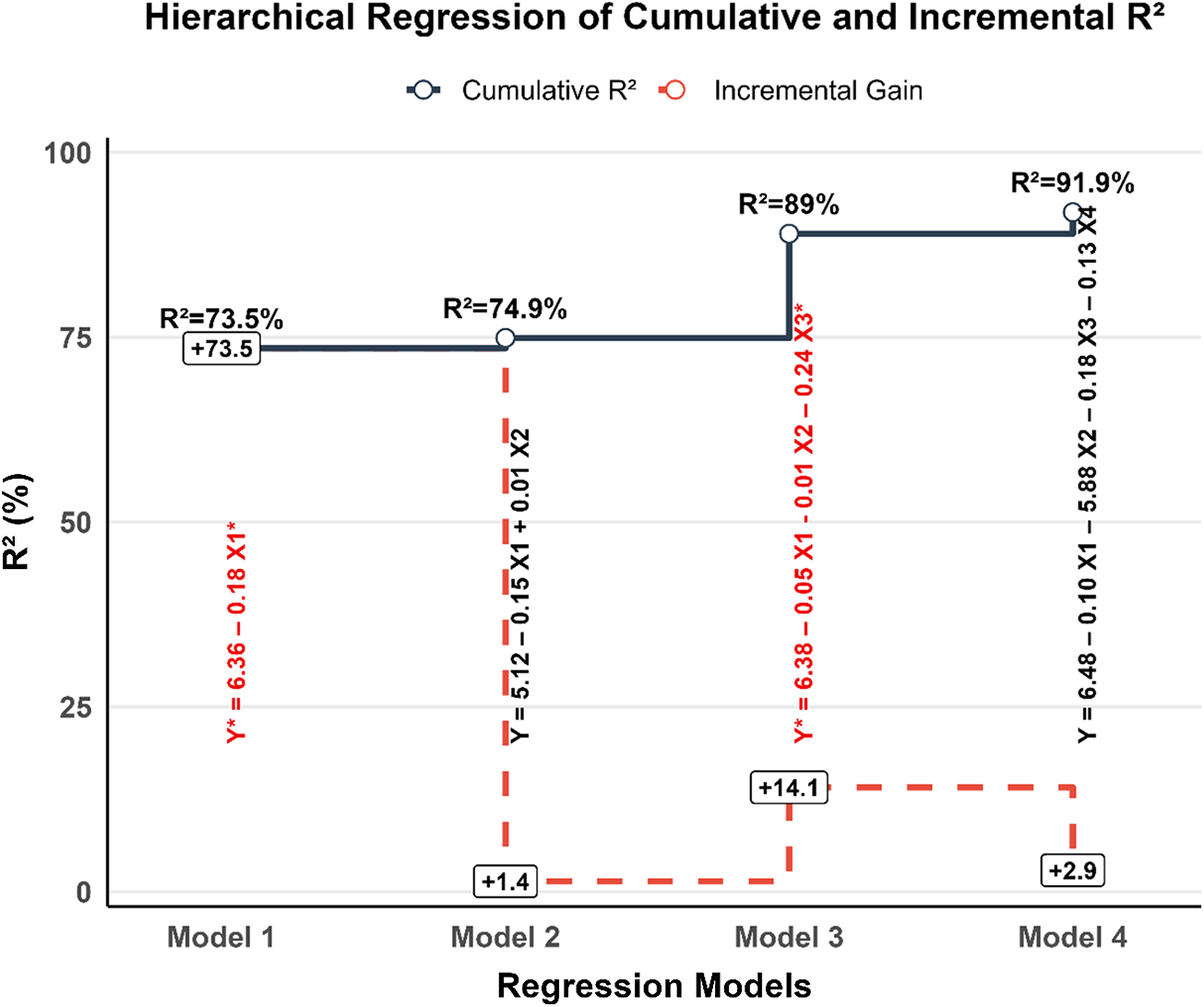
The hierarchical regression model (fig. 11) emphasised the relative importance of explanatory added-successive models (weather parameters) as the additional predictors introduced. The cumulative R 2, accounted for 73.5% increase in Model 1 (mean temperature) to 91.9% in Model 4, indicating that more variance in aphid population with extended model. The added parameters depicted succeeding improvement such as 1.4% in Model 2 (relative humidity), followed by 14.1% in Model 3 (sunshine hours) and 2.9% in Model 4 (rainfall). This indicates that temperature was the strongest single predictor, while inclusion of sunshine and rainfall further refined model accuracy.
Hierarchical regression models showing the coefficient of determination (R 2) and the contribution of individual weather factors to fluctuations in the wheat aphid population. Here, Y represents aphid population density; X 1 = weekly mean temperature (°C), X 2 = weekly mean relative humidity (%), X 3 = weekly hours of sunshine, and X 4 = weekly rainfall (mm) for each week; * = significant at P < 0.05 and ** = significant at P < 0.01.

Figure 11 Long description
The graph shows hierarchical regression models with cumulative and incremental R squared values. The x-axis is labeled 'Regression Models' and includes Model 1, Model 2, Model 3 and Model 4. The y-axis is labeled 'R squared (percent)'. Cumulative R squared values are marked with diamonds, showing 73.5 percent for Model 1, 74.9 percent for Model 2, 89 percent for Model 3 and 91.9 percent for Model 4. Incremental gains are marked with circles, showing plus 1.4 percent for Model 2, plus 14.1 percent for Model 3 and plus 2.9 percent for Model 4. Red dashed lines indicate incremental gains between models, with equations Y equals 0.65 minus 0.15 X subscript 1 for Model 2, Y equals 0.68 minus 0.06 X subscript 1 minus 0.04 X subscript 2 for Model 3 and Y equals 0.68 minus 0.06 X subscript 1 minus 0.03 X subscript 2 minus 0.03 X subscript 3 for Model 4.
Discussion
The present study highlights the complexity of aphid population dynamics in wheat, with significant differences in infestation levels among wheat genotypes and sampling periods (table 1: two-way factorial, P < 0.05), observed across the evaluated sowing dates under varying environmental conditions. Within all seven sowing dates, significant differences were detected among wheat genotypes, suggesting that host plant resistance or susceptibility plays a pivotal role in shaping aphid colonisation and development. Aphid abundance differed significantly among wheat genotypes (table 1: split plot design, P < 0.001), with higher mean densities observed on Arooj-22 (3.59), V-22426 (3.23), and V-7016S1 (3.10) compared with lower mean densities on V-19317 (2.76) and V-22647 (2.77). Such variability emphasises the importance of genotype selection as a fundamental component of integrated pest management (IPM). Previous studies have also accentuated that genotypic traits such as leaf surface morphology, nutritional quality, and plant vigour influence the attractiveness and suitability of host plants to aphids (Ali et al., Reference Ali, Naseem, Arshad, Ashraf, Rizwan, Tahir, Rizwan, Sayed, Ullah, Khan, Amir, Pan and Liu2021; Jiang et al., Reference Jiang, Cheng, Lu, Chen, Zhao and He2022). Our findings reinforce these observations and highlight the potential for incorporating resistant/tolerant lines in breeding programs to reduce pest pressure (Yahya et al., Reference Yahya, Saeed, Nadeem, Hamed and Shokat2017; Nawaz et al., Reference Nawaz, Khan, Dawar, Khalil, Hussain, Saad, Rasheed and Rahamdad2024).
Another critical outcome of this study is the clear temporal pattern of aphid infestation. Populations were highest at first three sample dates in February across most sowing dates and genotypes, with particularly high infestations observed on 20 and 27 February. This narrow but consistent window reflects the synchronisation between aphid life cycles and favourable environmental conditions. Cool temperatures combined with relatively high humidity during this period likely facilitated rapid aphid multiplication and colonisation. Similar temporal peaks have been reported in wheat-growing regions of South Asia and elsewhere, where aphid populations typically surge during cooler winter months before declining as temperatures rise in March (Nawaz et al., Reference Nawaz, Khan, Dawar, Khalil, Hussain, Saad, Rasheed and Rahamdad2024; Hameed et al., Reference Hameed, Muhammad and Shah2025). Recognising these vulnerable windows is vital for farmers and extension workers, as it provides a strategic basis for timing pest monitoring and intervention efforts. Early warning systems can therefore be built around this knowledge, helping to minimise yield losses while reducing unnecessary pesticide applications.
The association of aphids with natural enemies further illustrates the ecological dynamics at play. In the present study, significant correlations were observed between aphid populations and their key biological control agents conclusively, Coccinellids, Chrysopids, syrphids, and parasitoids. Although the strength of association varied across dates, the positive relationships indicate that natural enemy populations tracked aphid density, suggesting density-dependent regulation. This finding aligns with the classic ecological principle that natural enemies often respond numerically or functionally to prey abundance (Snyder, Reference Snyder2019). For instance, syrphid larvae and coccinellid beetles are known to increase in numbers with rising aphid densities, thereby exerting a natural suppressive effect (Brown, Reference Brown, Hodek, van Emden and Honěk2012). However, the exceptions observed in our dataset; for example, non-significant associations of coccinellids and parasitoids on 14 February, suggest that the natural enemies may lag behind aphid population peaks, or that other ecological constraints (such as temperature or alternative prey availability) influenced their activity. This temporal mismatch may reduce the immediate effectiveness of biological control during critical periods of aphid outbreak, emphasising the need for conservation practices that enhance the early build-up of beneficial insects (Brown, Reference Brown, Hodek, van Emden and Honěk2012).
Equally important are the abiotic drivers of aphid dynamics. Our results demonstrated a strong and consistent negative association between aphid populations and both mean temperature and sunshine hours, while relative humidity exhibited a significant positive relationship (except for sowing dates V and VI). Hierarchical regression analysis was used to assess the relative and incremental contribution of measured abiotic variables to variation in aphid abundance. Mean temperature accounted for the largest proportion of explained variance, while the sequential inclusion of relative humidity, hours of sunshine, and rainfall resulted in additional increases in model fit. These results indicate strong statistical associations between aphid abundance and prevailing abiotic conditions (temperature as most influential factor, accounting for 73.5%); however, they do not imply direct causal or regulatory effects. These findings are consistent with the well-documented preference of aphids for cooler, humid conditions that favour their survival, reproduction, and development (Khakwani et al., Reference Khakwani, Dennett, Munir and Abid2012; Singh et al., Reference Singh, Simon, Halsey, Kurup, Clark and Aradottir2020). Conversely, higher temperatures and longer sunshine exposure likely create stressful conditions that reduce survival or accelerate the decline of aphid colonies. The positive role of relative humidity is particularly relevant in the context of changing climate scenarios, as shifts in weather patterns may influence pest pressure in ways that are currently underappreciated. Integrating such ecological insights into pest forecasting models can greatly improve predictive accuracy and preparedness.
From a management perspective, the implications of this study are multifaceted. First, sowing date is a critical determinant of pest pressure. Early- or late-sown crops may experience lower aphid densities compared to crops sown in the first half of December, which coincides with conditions favouring pest build-up in February. Adjusting sowing schedules could therefore serve as a cultural control measure that minimises the risk of peak infestation. Second, the identification of relatively resistant genotypes such as V-19317 and V-22647 offers breeders and farmers practical options for reducing aphid vulnerability. These genotypes could either be promoted directly or serve as parent material for breeding resistant cultivars. Third, the apparent ability of natural enemies to track aphid abundance supports the adoption of ecological engineering practices such as planting nectar-rich borders, reducing broad-spectrum pesticide use, and promoting habitat heterogeneity to conserve and enhance biological control agents. By fostering early activity and higher abundance of predators and parasitoids, the reliance on chemical interventions can be substantially reduced.
It is also worth-noting that while chemical control remains a common farmer practice, over-reliance on insecticides poses risks of resistance development, environmental contamination, and disruption of beneficial arthropod populations. Our findings suggest that targeted insecticide applications, if necessary, should be confined to the peak infestation window (14–27 February) and only when aphid populations exceed economic threshold levels. Such an approach would not only enhance the effectiveness of chemical interventions but also reduce the negative ecological and economic consequences of indiscriminate spraying. The integration of host plant resistance, adjusted sowing time, conservation of natural enemies, and climate-informed forecasting provides a robust framework for sustainable aphid management.
Conclusion
The present study demonstrated that aphid population dynamics in wheat are significantly influenced by sowing date, genotype, and environmental factors. Across sowing dates, considerable variation was observed, with certain genotypes such as Arooj-22, V-22426, and V-7016S1 consistently showing higher susceptibility, while others such as V-19317 and V-22647 maintained relatively lower infestation levels. Aphid pressure peaked during mid to late February (14–27 February), highlighting this period as the most vulnerable window for infestation.
The strong positive association between aphid abundance and relative humidity, along with the negative relationship with temperature and hours of sunshine, clearly indicates that cooler, humid conditions favour aphid outbreaks by enhancing survival, reproduction, and nymphal development while reducing desiccation stress, leading to rapid population build-up. Moreover, natural enemies, including Coccinellids, Chrysopids, Syrphids, and parasitoids, showed significant correlations with aphid population dynamics, suggesting they play a role in natural regulation. Hierarchical regression analysis confirmed temperature as the dominant factor explaining up to 73.5% of aphid population fluctuation, followed by sunshine hours and relative humidity.
Acknowledgements
The authors would like to acknowledge the Deanship of Graduate Studies and Scientific Research, Taif University for supporting this work.
Author contributions
Faisal Hafeez: Conceptualisation, Writing original draft, Methodology, Investigation, Formal analysis, Data Curation, Writing Review and Editing. Javed Ahmad: Supervision, Resources and Writing-Review and Editing. Ayesha Iftikhar: Methodology, critically revised the manuscript. Arzlan Abbas: Writing-Review and Editing. Manel Ben Ali: Funding and reviewing. Fehmi Boufahja: Funding and editing. Muhammad Zulkiffal: Data curation and methodology. Muhammad Ilyas Khakhar: Writing original draft. Amor Hedfi: Funding, formal analysis and supporting. Majid Nadeem: Methodology and Writing-Review and Editing. All authors have read and agreed to the published version of the manuscript.
Competing interests
The author(s) declare that they have no conflict of Interest.
Ethical approval
Not applicable.
Availability of data and materials
Not applicable.