1. Introduction
We consider the flow within a rotating fluid-filled torus from a computational perspective. The flow that develops as a result of an impulsive change in the rotation rate of the torus provides a paradigm for the study of collisional boundary layers and unsteady boundary-layer separation. The phenomena of collisional boundary layers has been extensively studied over the past thirty years. Early work of Banks & Zaturska (Reference Banks and Zaturska1979) considered the asymptotic structure that arises in the flow near the equator of an impulsively rotated sphere, demonstrating that the flow exhibits all the hallmarks of a finite-time singularity. This result was subsequently confirmed by Stewartson, Cebeci & Chang (Reference Stewartson, Cebeci and Chang1980). The finite-time singularity, which manifests itself physically as a rapid thickening of the boundary layer, has since been shown to occur in a wider range of important fluid flows. Dennis & Duck (Reference Dennis and Duck1988) demonstrated that such finite-time singularities also develop when a sphere, immersed in a body of fluid, is impulsively rotated.
In addition to these external flows, boundary-layer collisions also arise in internal flows. Perhaps the most accessible and well-studied example results from the starting flow in a curved pipe, a flow that has a number of applications in physiology (see Pedley Reference Pedley2003, for a discussion of the relevance of this flow to that in the aortic arch). The imposition of a constant pressure gradient results in the collision of boundary layers at the inside bend of the pipe, a collision which is manifest in a finite-time singularity (Riley Reference Riley1998). A similar phenomena arises in the entry flow in a curved duct, manifesting as a rapid thickening of the boundary layer on the duct wall, as shown by Stewartson et al. (Reference Stewartson, Cebeci and Chang1980). Experimental evidence for this collision process, and the subsequent boundary-layer singularity, can be found in Kluwick & Wohlfahrt (Reference Kluwick and Wohlfahrt1986) (for the entry flow in a curved duct) and Boirin, Deplano & Pelissier (Reference Boirin, Deplano and Pelissier2006) (for the problem of the starting flow in curved duct). In both problems, results from experiments, computation and asymptotic analysis can be drawn together to provide a description of the boundary-layer development, subsequent collision and eruption. The structure of the flow after this collision event is, however, less clear.
In addition to the aforementioned work there is another class of fluid flows that demonstrates all of the hallmarks of a boundary-layer collision. Such phenomena occur within a fluid-filled torus suddenly rotated from rest to a state of rigid-body rotation. This class of toroidal flows has a number of important applications, for example in toroidal dynamo flows (see Noskov et al. Reference Noskov, Stepanov, Denisov, Frick, Verhille, Pilhon and Pinton2009). Experiments by Madden & Mullin (Reference Madden and Mullin1994) on the flow within a suddenly rotated torus demonstrate the rich and complex dynamics that can arise in this class of unsteady flows, including a transition to a transient turbulent state as the flow evolves to a (stable) state of rigid-body rotation.
Many of the experimentally observed features of this flow were subsequently explored using a mix of computational and asymptotic methods by Hewitt et al. (Reference Hewitt, Hazel, Clarke and Denier2011) (also building upon further experimental work by del Pino et al.
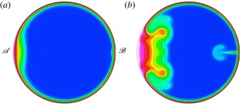
Reference del Pino, Hewitt, Clarke, Mullin and Denier2008). In particular, Hewitt et al. (Reference Hewitt, Hazel, Clarke and Denier2011) demonstrated that the boundary layers that develop within the flow, as a result of the impulsive change in rotation rate, collide and erupt as a result of a finite-time singularity. The position at which this phenomenon occurs depends upon the initial and final angular velocity. For example, in a flow spun up from rest, the eruption will occur at the outer radius of the torus, whereas in a flow spun down from rest, the eruption occurs at the inner radius of the torus. For ease of reference we will refer to these locations as
 $\mathscr{A}$
(outer) and
 $\mathscr{B}$
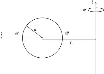
(inner), as indicated in figure 1. Eruptions resulting from finite-time singularities can also occur at both inner and outer radii, albeit at different times, if the direction of rotation is changed impulsively. Hewitt et al. (Reference Hewitt, Hazel, Clarke and Denier2011) provided strong evidence that this finite-time singularity coincided with the development of an observable band in the top-down flow visualisation experiments of Madden & Mullin (Reference Madden and Mullin1994).
The experiments by Madden & Mullin (Reference Madden and Mullin1994) and del Pino et al. (Reference del Pino, Hewitt, Clarke, Mullin and Denier2008) also show a second band developing on the opposite equator to the first front. For example, when the finite-time singularity manifests at point
 $\mathscr{A}$
in the Madden & Mullin (Reference Madden and Mullin1994) experiment, a second laminar band is also observed at point
 $\mathscr{B}$
. Hewitt et al. (Reference Hewitt, Hazel, Clarke and Denier2011) showed that the boundary layers on the opposite equator were subject to an axisymmetric centrifugal instability that could be triggered by an isolated wall perturbation. Furthermore, for typical laboratory flows, it was found that the time scales of this centrifugal instability and the boundary-layer eruption were similar. Here, we show that a geometric imperfection in the torus surface, such as a small seam, could provide the mechanism for the development of the experimentally observed front. The resulting dynamics are different from that arising in the conjectured centrifugal instability of Hewitt et al. (Reference Hewitt, Hazel, Clarke and Denier2011).
2. Spin-down to rest
We consider the flow of a fluid within a torus of circular cross-section. The torus has a centreline (major) radius
 $L$
and cross-sectional (minor) radius
 $a$
, and is filled with an incompressible viscous fluid of kinematic viscosity
 ${\it\nu}$
(see figure 1). Initially the fluid and torus system are in a state of rigid-body rotation. At time
 $t=0$
an unsteady flow is generated by an impulsive change in the rotation rate of the torus.
A schematic of the torus, showing the cylindrical polar coordinate system, with dimensional centreline radius
 $L$
and cross-sectional radius
 $a$
. In our dimensionless coordinate system, the outermost point of the torus is at
 $r={\it\delta}^{-1}+1$
(point
 $\mathscr{A}$
), whilst the innermost point is at
 $r={\it\delta}^{-1}-1$
(point
 $\mathscr{B}$
), where
 ${\it\delta}=a/L$
is a non-dimensional curvature parameter.

Letting
 ${\it\Omega}_{i}$
denote the initial angular velocity of the torus and
 ${\it\Omega}_{f}$
the final angular velocity, we choose to non-dimensionalise the system by defining a typical length scale to be the radius
 $a$
of the inner toroidal cross-section, and a typical time scale to be
 ${\it\Omega}_{i}^{-1}$
(or equivalently a typical velocity scale
 $L{\it\Omega}_{i}$
). With this non-dimensionalisation the flow Reynolds number
 $\mathit{Re}$
is given by
 $$\begin{eqnarray}\mathit{Re}=\frac{aL{\it\Omega}_{i}}{{\it\nu}}.\end{eqnarray}$$
Let the dimensionless velocity components corresponding to the coordinates
 $(r,{\it\phi},z)$
be denoted by
 $(u,w,v)$
, and in what follows we will suppose that the fluid within the torus is initially in a state of rigid-body rotation so that
 $$\begin{eqnarray}u=v=0,\quad w=r\quad \text{at }t=0.\end{eqnarray}$$
We therefore focus on flow in which the boundary conditions for
 $t>0$
are that the torus rotates at the new frequency:
 $$\begin{eqnarray}u=v=0,\quad w={\it\Omega}(t)r\quad \text{on }z^{2}+(r-{\it\delta}^{-1})^{2}=1.\end{eqnarray}$$
We chose the linear ‘ramp-down’ profile
 $$\begin{eqnarray}{\it\Omega}(t)=1-\frac{2t}{\sqrt{\left(t_{s}-t\right)^{2}}+t_{s}+t},\end{eqnarray}$$
in which
 $t_{s}$
is the non-dimensional time taken for the annulus to spin down from its initial angular frequency
 ${\it\Omega}_{i}$
to its final angular frequency
 ${\it\Omega}_{f}=0$
(previous studies have shown that the flow is largely insensitive to the precise nature of the deceleration profile, see del Pino et al.
Reference del Pino, Hewitt, Clarke, Mullin and Denier2008).
We begin our investigation by considering the initial response to the change in rotation rate; namely, the development of a suddenly generated axisymmetric boundary layer, adjacent to the annular wall. The flow response will depend on three parameters: (i) the Reynolds number
 $\mathit{Re}$
; (ii) the ‘ramp-down’ parameter
 ${\it\beta}={\it\Omega}_{i}\hat{t}_{s}$
; and (iii) the curvature of the pipe
 ${\it\delta}=a/L$
. We choose values of
 ${\it\delta}=0.2$
and
 ${\it\beta}=0.7$
for all our spin-down computations.
2.1. Computational method
We assume that the flow is rotationally symmetric. Thus, all field variables are taken to be independent of the azimuthal angle
 ${\it\phi}$
(refer to figure 1). In this case the Navier–Stokes equations can be reduced to their rotationally symmetric form. These are discretised using quadrilateral spectral elements, as exploited in the package Semtex, whose capabilities are well suited to flows involving cylindrical coordinate systems (see Blackburn & Sherwin Reference Blackburn and Sherwin2004, for details). In particular Semtex uses parametrically mapped quadrilateral elements (thus ensuring that all elemental boundaries are curved and can be exactly matched to the ‘circular’ cross-sections considered here), the classic Gauss–Lobatto–Legendre ‘nodal’ shape function basis, and continuous Galerkin projection.
All computations reported here used a mesh of 504 elements (506 for the ‘seamed’ meshes), with each element containing an internal grid of
 $21\times 21$
Lagrange knot points. In order to accurately capture the dynamics of the colliding boundary layers, which occur at the equator, our mesh was designed to ensure the greatest resolution around the circumference of the cross-section and along the equator. Extensive convergence tests were conducted (for the highest Reynolds numbers reported here, 7800) and all the results presented are converged to within graphical accuracy for this largest Reynolds number. In all our calculations the temporal time stepping is accomplished via a second-order backwards-differencing scheme (for full details see Blackburn & Sherwin Reference Blackburn and Sherwin2004); for our calculations the time step
 ${\rm\Delta}t$
was set to 0.0001, convergence tests demonstrate that this is more than sufficient to ensure a converged solution for the most energetic flows considered.
2.2. Results
Spin-down simulations were run for various Reynolds numbers, with and without a seam at the equator (point
 $\mathscr{A}$
in figure 1). In the experiments of Madden & Mullin (Reference Madden and Mullin1994) the torus is manufactured in two halves, possibly introducing a geometric imperfection at the equator when the torus is bolted together, the exact form and size of which is difficult to determine. We will explore this issue by modelling the seam as a square cavity with side length
 $0.05a$
. In an accurately manufactured torus, such as that used by Madden & Mullin (Reference Madden and Mullin1994), we expect the seam to be smaller than this, but in order to facilitate efficient computations we need to ensure a balance between seam size against resolution. We return to this point in § 3.
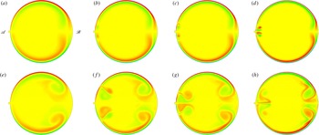
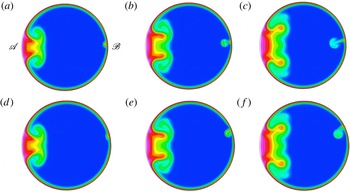
Contour plots of the cross-plane component of vorticity. Results for (a–d)
 $t=2$
and (e–h)
 $t=4$
for four different Reynolds numbers (a,e)
 $\mathit{Re}=1700$
, (b,f)
 $\mathit{Re}=2950$
, (c,g)
 $\mathit{Re}=3700$
, (d,h)
 $\mathit{Re}=7700$
. Here red denotes positive, yellow zero and green negative vorticity values respectively.

Figure 2 shows the azimuthal vorticity for various Reynolds numbers at times
 $t=2$
(a–d) and
 $t=4$
(e–h). The results for the first three Reynolds numbers (a,e)
 $\mathit{Re}=1700$
, (b,f)
 $\mathit{Re}=2950$
and (c,g)
 $\mathit{Re}=3700$
show the thinning of the wall boundary layer and the subsequent intensification of the post-collisional vortices (at point
 $\mathscr{B}$
) with increasing Reynolds number; however, the similarity in the post-collisional vortices is clearly apparent.
The same is not true for the vortices generated at point
 $\mathscr{A}$
. For
 $\mathit{Re}=1700$
figure 2(a,e) no vortex is generated at this location, the flow very closely resembling that of the ‘seamless’ torus. Comparing these results to those for
 $\mathit{Re}=2950$
figure 2(b,f), in which the ‘seam’ vortices are present, supports a Görtler-like vortex receptivity mechanism; for the lower Reynolds number the corresponding Görtler number of the flow is not large enough to allow for linearly unstable Görtler vortices. As the Reynolds number increases, to
 $\mathit{Re}=3700$
figure 2(c,g), the ‘seam’ vortices intensify, with the vortex roll-up occurring closer to the equator. The plots in figure 2(d,h) are for a Reynolds number of
 $\mathit{Re}=7700$
. Here we see an intensification of the post-collision vortices, and clear evidence of the development of a secondary vortex at location
 $r={\it\delta}^{-1}-1$
(point
 $\mathscr{B}$
). However, it is the ‘seam’ vortices that are the most dramatically modified. At time
 $t=2$
we observe a pair of counter-rotating vortices centred on the seam location, which appear to emanate from the seam. The vortex structure at the later time
 $t=4$
is now entirely different from that which develops at lower Reynolds numbers; the regions of positive and negative vorticity are now interchanged. Comparing figure 2(f) and (h) we observe that the ‘seam’ vortex is rotating in the opposite sense to the vortices observed at lower Reynolds numbers, indicating that the flow receptivity mechanism has changed from that which operates at lower Reynolds numbers.
3. Spin-up from rest
Although the results of Hewitt et al. (Reference Hewitt, Hazel, Clarke and Denier2011) suggest that the flow would be highly receptive to Görtler-like vortices, our results for the case of spin-down are somewhat surprising in that a small seam produces a significant global response in the flow and that this global response is significantly modified with increasing Reynolds number (in the sense that the flow receptivity no longer produces a Görtler-like vortex, but one with a different sense of rotation that we conjecture is driven by a second boundary-layer separation which occurs at the opposite equator to the collisional boundary-layer eruption).
We explore this issue of flow receptivity further by considering the spin-up problem (which is the less energetic flow regime). We proceed by assuming that the system is initially in a state of rest so that
 $$\begin{eqnarray}u=v=w=0\quad \text{at }t=0.\end{eqnarray}$$
In order to model the spin-up to a final, steady, angular frequency, we impose the boundary conditions, for
 $t>0$
,
 $$\begin{eqnarray}\displaystyle u=v=0,\quad w={\it\Omega}(t)r\quad \text{on }z^{2}+(r-{\it\delta}^{-1})^{2}=1, & & \displaystyle\end{eqnarray}$$
where
 ${\it\Omega}(t)$
, the linear ‘ramp-up’ profile, is given by
 $$\begin{eqnarray}{\it\Omega}(t)=\frac{2t}{\sqrt{\left(t_{s}-t\right)^{2}}+t_{s}+t},\end{eqnarray}$$
in which
 $t_{s}$
is the non-dimensional time taken for the annulus to spin up to its final angular frequency
 ${\it\Omega}_{f}$
. The Reynolds number
 $\mathit{Re}$
for the flow is now defined with respect to the angular frequency
 ${\it\Omega}_{f}$
as
 $$\begin{eqnarray}\mathit{Re}=\frac{aL{\it\Omega}_{f}}{{\it\nu}}.\end{eqnarray}$$
As the earlier experimental work of Madden & Mullin (Reference Madden and Mullin1994), and the subsequent work by Hewitt et al. (Reference Hewitt, Hazel, Clarke and Denier2011), used a toroidal pipe of radius
 $a=16\pm 0.1~\text{mm}$
and centreline radius of curvature
 $L=125\pm 0.1~\text{mm}$
, leading to a curvature parameter
 ${\it\delta}=0.128$
, we shall use this value for all our results in this section. This provides another useful check of our numerics against those of Hewitt et al. (Reference Hewitt, Hazel, Clarke and Denier2011), thus demonstrating the generic nature of the flow features (i.e. they are effectively independent of the value of
 ${\it\delta}$
albeit arising for different Reynolds numbers).
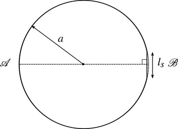
To quantify the effect of slight geometric imperfections on the flow we consider geometries in which the circular cross-section has a small ‘slice’ removed from the inner wall of the torus, as shown schematically in figure 3. In this figure the slice, of length
 $l_{s}$
, is taken perpendicular to the centreline and hence is symmetric about the
 $r$
-axis. Note that the slice position, at point
 $\mathscr{B}$
, has been chosen (initially) to be at the opposite side to the location at which the boundary-layer collision will occur during the spin-up from rest (see Hewitt et al.
Reference Hewitt, Hazel, Clarke and Denier2011, and also figure 4). We explore the effect of this geometric imperfection on the flow, and also the role that the position of the imperfection has upon the subsequent dynamics.
A schematic of the ‘sliced’ toroidal cross-section, where
 $l_{s}$
denotes the non-dimensional length of the slice.

3.1. Symmetric slice computations
The results we report are for the flow in which the torus is started from rest and spun up to a final angular frequency
 ${\it\Omega}_{f}=2~\text{s}^{-1}$
over a ramp-up time of
 $t_{s}=2$
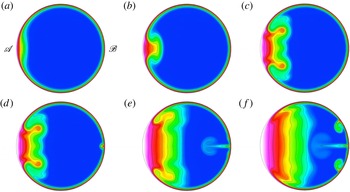
. Representative results showing the azimuthal velocity component, for the case when
 $l_{s}=0$
(i.e. a full circular cross-section), are presented in figure 4(a–c). Here the Reynolds number is set to be
 $\mathit{Re}=7800$
. As expected from the theoretical work of Hewitt et al. (Reference Hewitt, Hazel, Clarke and Denier2011), the spin-up process produces boundary layers which collide at point
 $\mathscr{A}$
and subsequently erupt, as a result of a finite-time singularity developing in the boundary-layer equations. The characteristic signature of the eruption is seen in figure 4(a), with a thickening of the boundary layer at point
 $\mathscr{A}$
, producing a distinctive ‘mushroom’ profile which thickens and expands until ultimately the flow achieves a state of rigid-body rotation (not shown here). We also note from this figure that the boundary layer at
 $r={\it\delta}^{-1}-1$
(point
 $\mathscr{B}$
) rapidly achieves a constant thickness, in agreement with the steady-state boundary-layer predictions of Hewitt et al. (Reference Hewitt, Hazel, Clarke and Denier2011). Thus, in the absence of a geometric perturbation, the flow develops entirely as predicted by Hewitt et al. (Reference Hewitt, Hazel, Clarke and Denier2011).
Contour plots of the azimuthal velocity component
 $w$
for slice length
 $l_{s}=0$
for times (a)
 $t=4$
, (b)
 $t=4.8$
, (c)
 $t=7.2$
and
 $l_{s}=0.025$
for times (d)
 $t=7.2$
(e)
 $t=11.2$
and (f)
 $t=14$
. The flow Reynolds number is
 $\mathit{Re}=7200$
.

We now consider the ‘sliced’ cross-section for various slice lengths;
 $l_{s}=0.025,0.05,0.1$
and 0.2. Figure 4(d–f) shows contours of the azimuthal velocity for the case
 $l_{s}=0.025$
. Up until
 $t\approx 6.8$
, the flow is indistinguishable from the case with a true circular cross-section. It is only after this that we see any divergence between the behaviour of the two flows. Comparing figure 4(c) with 4(d) (both for
 $t=7.2$
) we see a thickening of the boundary layer at point
 $\mathscr{B}$
, which by
 $t=11.2$
(figure 4
e) has resulted in an equatorial jet that has almost reached the centre of the torus’ cross-section. At this particular instant, the jet has had little impact upon the global features of the flow, which are still dominated by the post-collision vortices emanating from point
 $\mathscr{A}$
. A slight bulging in the boundary layer either side of the jet stem develops further into a pair of vortices which serve to transport vorticity towards the poles, figure 4(f). At this later time
 $t=14.0$
, the advancing front from the boundary-layer collision now interacts with the erupting jet, the front now being deformed by the presence of the jet. This competition between jet growth and the development of the flow towards a rigid-body rotation, serves to enhance the two smaller vortices, driving these further towards the polar regions. Increasing the slice length to
 $l_{s}=0.1$
reduces the time at which the jet develops, as can be seen in the two images presented in figure 5, but otherwise leaving the flow unchanged (compare figures 4
c,d and 5
b).
Contour plots of the azimuthal velocity component
 $w$
for a sliced cross-section (
 $l_{s}=0.1$
) at times (a)
 $t=4.0$
and (b)
 $t=7.2$
for a flow with a Reynolds number
 $\mathit{Re}=7800$
.

The development of the jet with increasing
 $l_{s}$
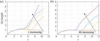
and Reynolds number is represented in figure 6, where we present plots of the jet length, measured from the torus wall at
 $r={\it\delta}^{-1}-1$
(point
 $\mathscr{B}$
) to the end of the jet (here defined as being the point on the equator at which the azimuthal velocity component in the jet is within
 $0.01$
of the surrounding quiescent fluid). This measure also captures the thickening of the wall boundary layer, as is seen in figure 6(a), which shows results for varying
 $l_{s}$
at a fixed Reynolds number of
 $\mathit{Re}=7800$
. The case
 $l_{s}=0$
shows the typical temporal growth of the boundary layer, as was predicted by Hewitt et al. (Reference Hewitt, Hazel, Clarke and Denier2011), the boundary layer rapidly settling down to a steady-state value. The development of the jet is seen, deviating further from the steady
 $l_{s}=0$
result at earlier times as
 $l_{s}$
is increased. A similar trend is seen in figure 6(b), where the slice length is held fixed, here at
 $l_{s}=0.025$
, and the flow Reynolds number has been changed. A significant change in the dynamics occurs as we further increase
 $l_{s}$
, as evidenced by the plot of jet length (figure 6
a). For
 $l_{s}=0.2$
, for
 $t\gtrsim 6.2$
the jet length grows linearly with time, different from that seen for smaller
 $l_{s}$
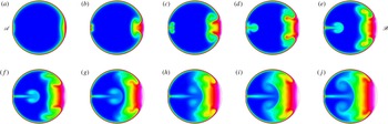
. The reason for this can be seen in the contour plots presented in figure 7. The early-time dynamics are similar, showing a slight bulging of the boundary layer at position
 $\mathscr{B}$
. However this structure does not immediately result in the jet seen in smaller
 $l_{s}$
simulations. The slice itself serves to redirect the flow within the wall boundary layer back to the equator, resulting in stretching of the jet. This stretching then serves to generate the secondary jet, seen in figure 7(c), with the jet ejection then serving to significantly modify the flow resulting from the equatorial boundary-layer collision (at point
 $\mathscr{A}$
).
In summary, the structure of the vortices observed for
 $l_{s}=0.025$
(figure 4
d–f) changes appreciably as we change the slice length. For this small slice length the vortices erupt from the boundary layer and are then advected towards the poles. Decreasing
 $l_{s}$
serves to generate more energetic poleward vortices. However, as we increase
 $l_{s}$
we find that the vortices become less intense and remain contained within the boundary layer (appearing as small deformations of the boundary layer) as they travel around the circumference of the cross-section, towards the equator at the outer wall.
Plots of the jet length (measured as multiples of the steady boundary-layer thickness
 ${\it\delta}_{s}$
) versus time for (a) the case of a Reynolds number
 $\mathit{Re}=7800$
and
 $l_{s}=0,0.025,0.05,0.1,0.2$
(the arrow showing the direction of increasing
 $l_{s}$
); (b) a slice length
 $l_{s}=0.025$
for Reynolds numbers
 $\mathit{Re}=3900,5850,7800,15\,600$
(the arrow showing the direction of increasing
 $\mathit{Re}$
).

Contour plots of the azimuthal velocity component
 $w$
for a sliced cross-section (
 $l_{s}=0.2$
) at times (a)
 $t=4.0$
, (b)
 $t=5.0$
, (c)
 $t=6.0,\dots \,$
( j)
 $t=13.0$
for a flow with a Reynolds number
 $\mathit{Re}=7800$
.

As noted earlier, the results of Hewitt et al. (Reference Hewitt, Hazel, Clarke and Denier2011) suggest that the flow in this location would be highly susceptible to centrifugal instabilities (i.e. Görtler-like vortices). This issue of flow susceptibility is best discussed in the context of flow receptivity. As was shown by Hewitt et al. (Reference Hewitt, Hazel, Clarke and Denier2011), the receptivity calculations of Denier, Hall & Seddougui (Reference Denier, Hall and Seddougui1991) can be used to explore the receptivity of this flow in the vicinity of the seam. Such a calculation shows a flow response in which the disturbance induced by a wall protuberance initially decays on the downstream side and then, after some suitable distance, grows again (as would be expected in the spatially developing flow – see for example figure 7 of Denier et al. (Reference Denier, Hall and Seddougui1991)), producing a wedge-like collection of counter-rotating vortices. This behaviour is also seen quite clearly in experiments conducted on the concave section of the NASA Langley Laminar Flow Wing in Mangalam, Dagenhart & Meyers (Reference Mangalam, Dagenhart and Meyers1985) (see also the image reproduced in figure 1.1 of Hall (Reference Hall1990)). In these experiments, sublimating chemicals were used to highlight the regions of high shear stress which develop due to the presence of the centrifugal instability; the regions so highlighted show the wedge-like form seen in the receptivity calculations.
A similar structure is seen in the simulations presented in Hewitt et al. (Reference Hewitt, Hazel, Clarke and Denier2011); see for example their figure 20, which presents contours of surface shear stress. In that case the vortices develop temporally, spreading out in the
 ${\it\theta}$
direction from
 ${\it\theta}=0$
. A linear evolution is clearly seen at smaller times (figure 20a), with the fuller nonlinear evolution seen at later times (figure 20b). The nonlinear evolution stage clearly shows the development of multiple counter-rotating vortex pairs. Recently Schrader, Brandt & Zaki (Reference Schrader, Brandt and Zaki2011) have demonstrated that receptivity to wall roughness is linear, even for ‘large’ roughness elements (up to 40 % of the local boundary-layer displacement thickness).
The flow dynamics near the ‘seam’ show no evidence of the typical signature of nonlinear Görlter vortices triggered through a surface roughness receptivity mechanism. We therefore conclude that the jet is not a manifestation of a centrifugal instability but demonstrates new dynamics for this class of flow.
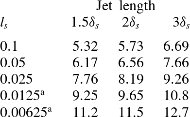
Data extracted from figure 6 showing the non-dimensional time
 $t$
corresponding to the jet lengths of
 $1.5{\it\delta}_{s}$
,
 $2{\it\delta}_{s}$
and
 $3{\it\delta}_{s}$
for different slice lengths
 $l_{s}$
.
 $^{\text{a}}$
The values indicated have been obtained by extrapolating from the data for slice lengths
 $l_{s}=0.1,0.05$
and 0.025 using linear regression.

It is worth exploring the effect of the decreasing seam size in some more detail. From a computational standpoint, it becomes increasingly difficult to resolve the flow structures due to the seam. We can, however, make some progress by making use of the data available for larger seam sizes, using this to infer important features of the flow dynamics as the seam size is further reduced.
Table 1 summarises the time at which the jet has lengths
 $1.5{\it\delta},2{\it\delta}$
and
 $3{\it\delta}$
, extracted from the data presented in figure 6. The last two data points in this table, for
 $l_{s}=0.0125$
and 0.00625, have been estimated using a simple linear extrapolation from the first three computed data points. Noting that the experiments of Madden & Mullin (Reference Madden and Mullin1994) used a torus with a radius
 $a=16~\text{mm}$
, the two smaller values for
 $l_{s}$
given in table 1 would translate to physical dimensions of
 $l_{s}^{\ast }=0.2~\text{mm}$
and
 $l_{s}^{\ast }=0.1~\text{mm}$
respectively, and thus fall within the machining tolerance quoted in Madden & Mullin (Reference Madden and Mullin1994).
We can therefore make use of these, albeit extrapolated, results to make some qualitative comparisons between our computational results and the experiments presented by Madden & Mullin (Reference Madden and Mullin1994). This is most readily achieved if we first note that the steady boundary-layer thickness
 ${\it\delta}_{s}=0.0875$
. Table 1 presents the non-dimensional times at which the jet has length
 $1.5{\it\delta}^{\ast }$
,
 $2{\it\delta}^{\ast }$
and
 $3{\it\delta}^{\ast }$
. The results presented in table 1 serve to demonstrate that, even at the smaller scales typically quoted as manufacturing tolerances, an imperfection at the torus equator has the potential to have a significant impact upon the resulting flow dynamics. Care should therefore be taken when both constructing such apparatus and reporting on experimental results if comparison between theory and experiment is to be most readily facilitated.
3.2. Off-centre slice computations
It is evident from the previous results that the presence of a ‘seam’ has a significant effect upon the global dynamics of the flow; the formation of both the jet and the subsequent vortices depend on the Reynolds number of the flow. More specifically, we find that, beneath a particular value of
 $\mathit{Re}$
, no ejection occurs. The flow is sensitive to any surface imperfections (see earlier and the results of Hewitt et al.
Reference Hewitt, Hazel, Clarke and Denier2011) and that a seam, however small, may provide a sufficient disturbance to change the global dynamics of the flow. From an experimental viewpoint, in order to control these global dynamics, one must necessarily control both the location of the seam and its size. For this particular flow a seam at the equator is undesirable.
We explore this issue further by considering the effect of the seam location on the subsequent dynamics. To do this we move the slice from the centreline of the cross-section so that it is now off-centre. We move the slice anti-clockwise around the circumference of the cross-section so that it is only partially over the centreline (shown in figure 8 a–c), and again so that it is completely above the equator (see figure 8 d–f).
Contour plots of the azimuthal velocity component
 $w$
for a cross-section with slice,
 $l_{s}=0.05$
, (a–c) partially over the centreline and (d–f) completely above the equator. (a,d)
 $t=5.6$
, (b,e)
 $t=6.4$
and (c,f)
 $t=7.2$
for a flow with a Reynolds number
 $\mathit{Re}=7800$
.

In both cases, there is no evidence of the developing jet, but evidence of the development of the vortex, in this case positioned on the ‘slice-side’ of the equator. The higher slice location results in a more pronounced vortex that sheds into the boundary layer. Extensive tests with other slice locations, dimensions and Reynolds numbers, demonstrate that if the slice is taken from the top or the outer walls of the torus cross-section, we do not see these effects. Thus, this receptivity mechanism seems confined to the inner wall of the cross-section and near to the equator.
4. Conclusions
We have presented new results detailing the post-collision velocity field within a fluid-filled torus and how this flow may be impacted by slight imperfections in the torus surface. Our new computational results presented here serve to validate the theoretical description of the collisional boundary layers presented in Hewitt et al. (Reference Hewitt, Hazel, Clarke and Denier2011). Our computational experiments also provide an alternative physical mechanism for the generation of the second front that appears in the original flow visualisation experiments of Madden & Mullin (Reference Madden and Mullin1994). Receptivity calculations performed by Hewitt et al. (Reference Hewitt, Hazel, Clarke and Denier2011) suggested that this second front is the consequence of the flow becoming receptive to Görtler vortices induced by localised roughness at the equator. However, our new results provide evidence of a much larger counter-rotating vortex pair than would be expected from a roughness-induced Görtler vortex, and argue for an alternate receptivity mechanism.
Ideally, future experiments should be designed to take into account the extreme sensitivity of the flow to geometric details of the equator. Evidence of this extreme sensitivity can be found in the recently reported experiments of Walbran, Cater & Clarke (Reference Walbran, Cater and Clarke2013).
Acknowledgements
J.P.D. gratefully acknowledges the support of a Royal Society of New Zealand Marsden Fund grant. SAWC is the recipient of a University of Auckland Doctoral Scholarship. This work was completed whilst TWM was visiting the University of Auckland and he gratefully acknowledges their hospitality. Computing time was provided through NeSI, New Zealand’s high-performance computing facility. We are grateful for the insightful comments of the referees, comments that served to improve the presentation of this paper.