1. Introduction
In recent studies of the turbulent nonlinear evolution of inertially unstable vortices and planar shear flows in rotating homogeneous fluids, we showed how to predict the equilibrated flows that emerge (see Kloosterziel, Carnevale & Orlandi Reference Kloosterziel, Carnevale and Orlandi2007a
; Kloosterziel, Orlandi & Carnevale Reference Kloosterziel, Orlandi and Carnevale2007b
; Carnevale et al.
Reference Carnevale, Kloosterziel, Orlandi and van Sommeren2011; Carnevale, Kloosterziel & Orlandi Reference Carnevale, Kloosterziel and Orlandi2013). These studies considered uniformly rotating systems, the
 $f$
-plane dynamics well-known from geophysical fluid dynamics. In a laboratory setting of flows in a basin rotating with angular velocity
 ${\it\Omega}$
, the Coriolis parameter
 $f=2{\it\Omega}$
, whereas in the context of geophysical mid-latitude ocean/atmosphere flows,
 ${\it\Omega}$
is replaced by the projection of the Earth’s angular velocity on the local vertical axis, i.e.
 $f=2{\it\Omega}\sin {\it\phi}$
with
 ${\it\Omega}$
the planetary angular velocity and
 ${\it\phi}$
latitude (see e.g. Pedlosky Reference Pedlosky1987). In this study, we attempt to make similar predictions for zonal shear flows near the equator using the well-known equatorial
 ${\it\beta}$
-plane approximation. The equatorial
 ${\it\beta}$
-plane is just a special case of the ‘mid-latitude’
 ${\it\beta}$
-plane approximation which comes about from an expansion around a latitude
 ${\it\phi}_{0}$
with the variable Coriolis parameter approximated by
 $f=f(y)=f_{0}+{\it\beta}y$
with
 $f_{0}=2{\it\Omega}\sin {\it\phi}_{0}$
,
 ${\it\beta}=2({\it\Omega}/R)\cos {\it\phi}_{0}$
,
 $y=R({\it\phi}-{\it\phi}_{0})$
and
 $R$
the planet’s radius. So
 $y$
is the distance measured from the latitude
 ${\it\phi}_{0}$
, to which we can assign a distance
 $y_{0}=R{\it\phi}_{0}$
away from the equator. The equatorial
 ${\it\beta}$
-plane (
 $f(y)={\it\beta}y$
) follows by taking
 ${\it\phi}_{0}=0$
.
In this study we do not allow for along-stream (
 $x$
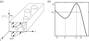
) variations. This restriction permits only the inertial instability to develop (see figure 1
a). Hence, we only consider ‘pure’ inertial instability, also known as ‘symmetric instability’ and as ‘centrifugal instability’ for circular flows. Further, we consider just a homogeneous fluid (constant density
 ${\it\rho}$
) and study the inertial instability of some barotropic flows with an initial zonal velocity
 $u=U(y)$
. For recent studies of the competition between inertial and barotropic instability see e.g. Gallaire & Chomaz (Reference Gallaire and Chomaz2003), Billant & Gallaire (Reference Billant and Gallaire2005), Griffiths (Reference Griffiths2008), Bouchut, Ribstein & Zeitlin (Reference Bouchut, Ribstein and Zeitlin2011), Carnevale et al. (Reference Carnevale, Kloosterziel, Orlandi and van Sommeren2011), Carnevale et al. (Reference Carnevale, Kloosterziel and Orlandi2013) and Ribstein, Plougonven & Zeitlin (Reference Ribstein, Plougonven and Zeitlin2014).
(a) Schematic showing a barotropic flow
 $u(y)$
and the vorticity produced by two types of instabilities (inertial and barotropic). With the equatorial
 ${\it\beta}$
-plane approximation the Coriolis parameter
 $f={\it\beta}y$
with
 $y$
latitude (south–north) and
 ${\it\beta}=2{\it\Omega}/R$
, with
 ${\it\Omega}$
the Earth’s angular velocity and
 $R$
the Earth’s radius. Horizontal vortex tubes (aligned along the
 $x$
-axis) represent pure inertial instability, and vertical vortex tubes (aligned along the
 $z$
-axis) represent pure barotropic horizontal-shear instability. Only pure inertial instability is considered in this study. (b) Schematic showing how to construct the predicted momentum distribution on the
 $f$
-plane with constant
 $f=f_{0}$
(from Kloosterziel et al.
Reference Kloosterziel, Orlandi and Carnevale2007b
). An initial distribution (thick solid curve) is unstable in the region
 $y_{-}<y<y_{+}$
where
 $\text{d}m/\text{d}y>0$
, taking
 $f_{0}>0$
. Equilibration sets
 $m=m_{c}$
over the wider range
 $y_{l}<y<y_{h}$
(thin curve).

With the imposed ‘symmetry’, for flows on the
 $f$
-plane we discovered (see Kloosterziel et al.
Reference Kloosterziel, Carnevale and Orlandi2007a
,Reference Kloosterziel, Orlandi and Carnevale
b
; Carnevale et al.
Reference Carnevale, Kloosterziel, Orlandi and van Sommeren2011, Reference Carnevale, Kloosterziel and Orlandi2013) that the outcome of inertial instability can often be predicted: although highly-nonlinear and turbulent the instability drives the flow towards a state of neutral stability through absolute momentum mixing. In the limit of large Reynolds numbers, the final state could be predicted based on the assumptions that (a) momentum is conserved and (b) the new flow that emerges is inertially stable. The basic idea is outlined in § 2 where we formulate the problem and outline some results from the literature concerning inertial instability.
In § 3 we study the evolution of an inertially unstable Gaussian jet centred on the equator flowing westward (an eastward flowing jet is inertially stable). In § 3.1 we present our prediction of the outcome of the instability. This prediction is well-confirmed in § 3.2 where we present the evolution of the instability for various Rossby numbers and Reynolds numbers through numerical simulations. Implicit in the prediction is that we assume that the adjusted momentum distribution has no discontinuities.
In § 4 we consider a uniform shear flow. This case has been widely studied in the past few decades because it always will be inertially unstable in some latitude band about the equator and because its simplicity allows for detailed linear stability analysis. In § 4.1 we show that, unlike for the Gaussian flow on the equatorial
 ${\it\beta}$
-plane or flows we studied before on the
 $f$
-plane (see Kloosterziel et al.
Reference Kloosterziel, Carnevale and Orlandi2007a
,Reference Kloosterziel, Orlandi and Carnevale
b
; Carnevale et al.
Reference Carnevale, Kloosterziel, Orlandi and van Sommeren2011, Reference Carnevale, Kloosterziel and Orlandi2013), there is an indeterminacy and no unique obvious prediction can be made through the simple construction of momentum redistribution. In § 4.2 we show through numerical simulations that ‘nature’ does drive the flow to a final state which is one of a multitude of possibilities, all of which must have at least one discontinuity in the adjusted profile. This leads to the question: is there something fundamentally different in the equatorial
 ${\it\beta}$
-plane dynamics from
 $f$
-plane dynamics? In other words, are there additional constraints hitherto never needed for
 $f$
-plane inertial instability that would provide a unique answer to the question of what the final flow should be? Could it be that the uniform shear case is somehow pathological? We have not been able to answer such questions. Nonetheless, the results are robust and may be a starting point for further investigation.
In § 5 we discuss the evolution of the Gaussian jet when the flow axis does not coincide with the equator. In that case the eastward flowing jet is also unstable and we show in § 5.1 how the final equilibrium can be predicted using the empirical results for the linear shear case from § 4. For larger shifts the equilibrated flow from the unstable eastward jet is predicted in § 5.2 with a simple construction which assumes continuity of the adjusted profile. The shifted westward Gaussian jet is discussed in § 5.3. For small shifts of the flow axis away from the equator no prediction appears possible. This is related to the fact that there is simultaneous inertial instability in two adjacent regions but with unequal rates of growth, unlike in § 3 where two adjacent regions of instability had equal growth rates.
For modest shifts we also show in § 5.3 that the equilibrium approaches a prediction which combines the results for the linear shear flow with a prediction similar to what we used in our previous studies for flows on the
 $f$
-plane. For large shifts of either jet, eastward or westward, the equilibrated flows on the
 ${\it\beta}$
-plane approach those reported in Kloosterziel et al. (Reference Kloosterziel, Orlandi and Carnevale2007b
) and Carnevale et al. (Reference Carnevale, Kloosterziel and Orlandi2013) where
 $f$
-plane dynamics was considered.
In § 6 we conclude with a brief discussion of the results and address various other unanswered questions. In the appendix A we explain the procedure with which we can predict the equilibrated flows that emerge from the eastward flowing jet with a small shift and the westward jet with a moderately small shift.
2. Formulation and background
Assuming no variability in the zonal
 $x$
-direction (west–east), the equations of motion for an incompressible, homogeneous fluid with the traditional approximation are
 $$\begin{eqnarray}\frac{\text{D}u}{\text{D}t}-f(y)v={\it\nu}{\rm\nabla}^{2}u,\quad \frac{\text{D}v}{\text{D}t}+f(y)u=-\frac{1}{{\it\rho}}\frac{\partial p}{\partial y}+{\it\nu}{\rm\nabla}^{2}v,\quad \frac{\text{D}w}{\text{D}t}=-\frac{1}{{\it\rho}}\frac{\partial p}{\partial z}+{\it\nu}{\rm\nabla}^{2}w\end{eqnarray}$$
and
 $$\begin{eqnarray}\frac{\partial v}{\partial y}+\frac{\partial w}{\partial z}=0.\end{eqnarray}$$
The material derivative and the Laplacian are
 $$\begin{eqnarray}\frac{\text{D}}{\text{D}t}=\frac{\partial }{\partial t}+v\frac{\partial }{\partial y}+w\frac{\partial }{\partial z},\quad {\rm\nabla}^{2}=\frac{\partial ^{2}}{\partial y^{2}}+\frac{\partial ^{2}}{\partial z^{2}}\end{eqnarray}$$
with
 $u,v,w$
the velocity components in the zonal
 $x$
-direction,
 $y$
-direction (south–north) and the vertical
 $z$
-direction, respectively. Here
 ${\it\rho}$
is the constant density,
 ${\it\nu}$
the kinematic viscosity,
 $p$
pressure and
 $t$
time. Although there are three velocity components, they only depend spatially on the cross-stream variable
 $y$
and the vertical variable
 $z$
. With the traditional approximation, horizontal and vertical accelerations due to the horizontal component of the Earth’s rotation vector are ignored and only horizontal motions are affected by rotation as in the usual
 $f$
-plane dynamics. But, in this study of equatorial flows, the variability of the Coriolis parameter
 $f(y)$
with latitude cannot be ignored.
Since we assume
 $\partial _{x}=0$
at all times, it follows that if viscosity vanishes, the absolute momentum
 $m$
is materially conserved:
 $$\begin{eqnarray}\frac{\text{D}m}{\text{D}t}=0\quad \text{with }m(y,z,t)=u(y,z,t)-\int ^{y}f(y^{\prime })\text{d}y^{\prime }.\end{eqnarray}$$
Apart from an arbitrary constant, the absolute momentum is
 $$\begin{eqnarray}\displaystyle \left.\begin{array}{@{}ll@{}}\text{mid-latitude }{\it\beta}\text{-}\text{plane:}~f(y)=f_{0}+{\it\beta}y, & m=u-f_{0}y-(1/2){\it\beta}y^{2},\\ \text{equatorial }{\it\beta}\text{-}\text{plane:}~f(y)={\it\beta}y, & m=u-(1/2){\it\beta}y^{2},\\ \text{mid-latitude }f\text{-}\text{plane:}~f(y)=f_{0}, & m=u-f_{0}y.\end{array}\right\} & & \displaystyle\end{eqnarray}$$
The stability of a stationary barotropic current with zonal velocity
 $u=U(y)$
with respect to ‘symmetric’ disturbances, i.e. disturbances that do not vary in the along-flow direction (
 $\partial /\partial x=0$
), is in the inviscid dynamics determined by the sign of the modified Rayleigh discriminant
 $$\begin{eqnarray}{\it\Phi}=f(\,f-\text{d}U/\text{d}y)=-f\text{d}M/\text{d}y\quad \text{with }M(y)=U(y)-\int ^{y}f(y^{\prime })\text{d}y^{\prime },\end{eqnarray}$$
with stability if
 ${\it\Phi}(y)\geqslant 0$
everywhere and instability if for some range of
 $y$
the discriminant
 ${\it\Phi}<0$
(see for circular flows Rayleigh Reference Rayleigh1916; Sawyer Reference Sawyer1947; Drazin & Reid Reference Drazin and Reid1981; Kloosterziel & van Heijst Reference Kloosterziel and van Heijst1991; Kloosterziel & Carnevale Reference Kloosterziel and Carnevale2007; Kloosterziel Reference Kloosterziel2010). For each particular approximation listed in (2.5), the appropriate combination of
 $f(y)$
and corresponding
 $M(y)$
must be used.
In terms of the absolute momentum, there will be stability if
 $f\text{d}M/\text{d}y<0$
for all
 $y$
and instability if
 $f\text{d}M/\text{d}y>0$
for some
 $y$
-range. For the mid-latitude
 $f$
-plane, the discriminant is
 ${\it\Phi}=f_{0}(\,f_{0}-\text{d}U/\text{d}y)$
with
 $f_{0}$
the Coriolis parameter and instability follows if
 $f_{0}\text{d}M/\text{d}y>0$
for some
 $y$
with
 $M=U(y)-f_{0}y$
(see Kloosterziel et al.
Reference Kloosterziel, Carnevale and Orlandi2007a
). Throughout the (mostly) meteorological literature, the more general criterion for symmetric instability in a continuously stratified fluid on the
 $f$
-plane is formulated as the condition that
 $f_{0}Q<0$
with
 $Q$
the Ertel potential vorticity (e.g. Fjortoft Reference Fjortoft1950; Ooyama Reference Ooyama1966; Hoskins Reference Hoskins1974; Holton Reference Holton1992). For the equatorial
 ${\it\beta}$
-plane see Griffiths (Reference Griffiths2003a
) and references therein. In this study of the evolution in a homogeneous fluid,
 $Q=f-\text{d}U/\text{d}y=-\text{d}M/\text{d}y$
is simply the absolute vertical vorticity, also called the potential vorticity.
In the limit of vanishing viscosity (
 ${\it\nu}=0$
or Reynolds number
 $\mathit{Re}\rightarrow \infty$
), the overturning motions associated with inertial instability amplify most rapidly if their vertical scales (i.e. in the
 $z$
-direction) are vanishingly small (e.g. Dunkerton Reference Dunkerton1981; Smyth & McWilliams Reference Smyth and McWilliams1998; Griffiths Reference Griffiths2008; Kloosterziel & Carnevale Reference Kloosterziel and Carnevale2008). The growth rate
 ${\it\gamma}$
of normal-modes perturbations, proportional to
 $\exp ({\it\gamma}t)$
, is bounded from above according to
 ${\it\gamma}<\sqrt{\max _{y}(-fQ)}$
provided that
 $fQ={\it\Phi}<0$
somewhere in the domain. This inviscid maximum growth rate is attained for infinitely shallow overturning motions, i.e. when vertical scales become vanishingly small. For finite but large enough Reynolds numbers, only perturbations with vertical scales within a finite range will amplify. Within this range, a maximum growth rate is found at a specific vertical scale. Hence, if a flow is subjected to small (symmetric) perturbations and the ‘fastest’ mode is excited, one expects meridional motions with this scale to emerge. For numerical simulations exhibiting this behaviour, see for example Griffiths (Reference Griffiths2003b
), Kloosterziel et al. (Reference Kloosterziel, Carnevale and Orlandi2007a
,Reference Kloosterziel, Orlandi and Carnevale
b
), Plougonven & Zeitlin (Reference Plougonven and Zeitlin2009) and Carnevale et al. (Reference Carnevale, Kloosterziel and Orlandi2013). These simulations showed that the initially orderly (normal-modes type) growth is followed by a turbulent phase in the evolution which ultimately results in a new, quasi-steady stable barotropic flow with
 $fQ\geqslant 0$
everywhere.
We discovered that the outcome of this highly nonlinear evolution on the
 $f$
-plane could be well predicted for high Reynolds numbers through a recipe for absolute (geostrophic) momentum mixing. The recipe is based on conservation of total (volume integrated) momentum
 $m=u-f_{0}y$
and the idea that at infinite Reynolds number mixing would be perfectly efficient, mixing uniformly in and around the instability region, and mixing no more momentum than is necessary to reach a stable equilibrium. A mixing of momentum to reach a uniformly mixed state over a range whose width is determined by conservation of total momentum is all that is needed to predict the final stable flow for large Reynolds numbers. Such flows have
 $f_{0}Q=-f_{0}\text{d}m/\text{d}y\geqslant 0$
everywhere. In the ‘mixed’ region that emerges the flow is neutrally stable, i.e.
 $\text{d}m/\text{d}y=0$
, while elsewhere
 $f_{0}\text{d}m/\text{d}y<0$
, as sketched in figure 1(b). The thin horizontal line between
 $y_{l}<y<y_{h}$
is the constant
 $m=m_{c}$
of the predicted inertially stable barotropic flow expected to emerge from the initial flow (thick solid line). Assuming
 $f_{0}>0$
, the initial flow is unstable in the region
 $y_{-}<y<y_{+}$
where
 $\text{d}m/\text{d}y>0$
and hence has
 $f_{0}Q<0$
in that region. Total momentum conservation simply requires that
 $$\begin{eqnarray}\int _{y_{l}}^{y_{h}}(m_{c}-m(y))\text{d}y=0,\end{eqnarray}$$
which, in a simple case such as that sketched in figure 1(b), uniquely determines
 $m_{c}$
,
 $y_{l}$
(
 $y$
low) and
 $y_{h}$
(
 $y$
high). For
 $y<y_{l}$
and
 $y>y_{h}$
, the momentum distribution remains unchanged. By construction, the predicted momentum distribution
 $m(y)$
has the same total momentum as the original unstable profile. In the region of constant
 $m=m_{c}$
(
 $y_{l}\leqslant y\leqslant y_{h}$
), the predicted equilibrated velocity is
 $u(y)=m_{c}+f_{0}y$
, while outside this region it is unchanged, i.e.
 $u(y)=U(y)$
.
An important difference between this study and our previous studies is that
 $f(y)={\it\beta}y$
changes sign going from ‘south’ (
 $y<0$
) to ‘north’ (
 $y>0$
) across the equator at
 $y=0$
, and
 $\text{d}m/\text{d}y>0$
no longer necessarily implies instability because instability is expected when
 $f(y)\text{d}m/\text{d}y>0$
(see for example figure 3
a and caption).
Below we present results from numerical simulations of the Navier–Stokes equations, i.e. (2.1a−c
) and (2.2) which are zonally invariant (no
 $x$
-dependence). The method of simulation is a channel model based on the staggered mesh scheme. The model is described in detail in Orlandi (Reference Orlandi2000). This numerical scheme conserves energy when run inviscidly, so energy dissipation should result only from the explicit viscosity. The computational domain in the
 $y$
-direction is terminated by free-slip vertical walls. Simulations with the flow periodic in the vertical direction were compared with simulations with free-slip boundaries in that direction. No significant differences were found, and we report only results with periodicity in the vertical here.
The initial velocity field was constructed from the basic velocity field
 $U(y)$
plus small random perturbations. The perturbations are applied in all three velocity components and at all points in the domain. Depending on the initial flow
 $U(y)$
,
 $f(y)$
and the demand that for given Reynolds number the instability is well-resolved, resolutions from
 $513\times 513$
up to
 $2049\times 2049$
grid points were used (details are in the text and figure captions).
3. A westward flowing Gaussian jet centred on the equator
As in Kloosterziel et al. (Reference Kloosterziel, Orlandi and Carnevale2007b ) and Carnevale et al. (Reference Carnevale, Kloosterziel and Orlandi2013), we first consider a barotropic current with streamwise velocity
 $$\begin{eqnarray}U(y)=U_{0}\exp (-y^{2}/L^{2}),\end{eqnarray}$$
with absolute momentum
 $m=M(y)=U(y)-{\it\beta}y^{2}/2$
. The length scale
 $L$
determines the width of the jet which is centred on the equator. Whereas on the
 $f$
-plane the sign of the peak velocity
 $U_{0}$
is irrelevant, on the equatorial
 ${\it\beta}$
-plane stability/instability does depend on the sign of
 $U_{0}$
. On the
 ${\it\beta}$
-plane, there will be instability if
 $\text{d}M/\text{d}y>0$
for
 $y>0$
but also when
 $\text{d}M/\text{d}y<0$
when
 $y<0$
because
 $f={\it\beta}y$
changes sign with
 $y$
.
In this section we use the length scale
 $L$
and the time scale
 $T=1/{\it\beta}L$
to non-dimensionalize all dimensional quantities. Thus the non-dimensional absolute momentum
 $M$
and non-dimensional initial velocity field
 $U(y)$
are
 $$\begin{eqnarray}M=\mathit{Ro}\exp (-y^{2})-\frac{y^{2}}{2},\quad U=\mathit{Ro}\exp (-y^{2}),\quad \text{with }\mathit{Ro}=\frac{U_{0}}{{\it\beta}L^{2}}\end{eqnarray}$$
the ‘equatorial’ Rossby number.
The condition for instability is
 ${\it\beta}y\,\text{d}M/\text{d}y>0$
or non-dimensionally
 $$\begin{eqnarray}y\,\text{d}M/\text{d}y>0\quad \text{with }\text{d}M/\text{d}y=-2y\mathit{Ro}\exp (-y^{2})-y.\end{eqnarray}$$
Equivalently the condition is that the Rayleigh discriminant
 ${\it\Phi}=-{\it\beta}y\text{d}M/\text{d}y<0$
, which we can write non-dimensionally as
 $$\begin{eqnarray}\tilde{{\it\Phi}}={\it\Phi}/{\it\Omega}^{2}=4(L/R)^{2}y^{2}(2\mathit{Ro}\exp (-y^{2})+1)<0\end{eqnarray}$$
(
 ${\it\Omega}$
is the planetary angular velocity). Hence, instability is not possible for positive
 $\mathit{Ro}$
because then
 $y\text{d}M/\text{d}y\leqslant 0$
or
 ${\it\Phi}>0$
for all
 $y$
. In other words: an eastward flowing jet (
 $U_{0}>0$
or
 $\mathit{Ro}>0$
) will be stable, and only a westward flowing jet with
 $U_{0}<0$
and
 $\mathit{Ro}<-1/2$
is expected to be unstable. Under terrestrial circumstances, this means (using
 $R\approx$
6380 km,
 ${\it\Omega}\approx 7.29\times 10^{-5}~\text{s}^{-1}$
) that for instability
 $$\begin{eqnarray}\text{for }L=25~\text{km:}\quad |U_{0}|>0.7~\text{cm}~\text{s}^{-1},\quad \text{for }L=50~\text{km:}\quad |U_{0}|>2.9~\text{cm}~\text{s}^{-1},\end{eqnarray}$$
and so on. In § 5 we will show that the eastward flowing jet is unstable when the axis of the flow does not exactly coincide with the equator.
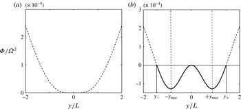
In figure 2(a), we show
 $\tilde{{\it\Phi}}$
for the critical
 $\mathit{Ro}=-1/2$
when for all
 $y$
the discriminant
 $\tilde{{\it\Phi}}\geqslant 0$
. In figure 2(b), we show
 $\tilde{{\it\Phi}}$
for
 $\mathit{Ro}=-4$
when the jet is expected to be unstable. There are two regions of instability where
 $\tilde{{\it\Phi}}<0$
, joined at
 $y=0$
. Roughly in the middle of each region, maximal negative
 $\tilde{{\it\Phi}}$
is found at
 $y=\pm y_{max}$
. These are the positions of maximal growth of the symmetric instability. The non-dimensional value of
 $y_{max}$
is determined by the relation
 $$\begin{eqnarray}2|\mathit{Ro}|(1-y^{2})=\exp (y^{2}).\end{eqnarray}$$
The outer edges of the instability regions are indicated by
 $y_{\pm }$
where
 $\tilde{{\it\Phi}}=0$
or
 $\text{d}M/\text{d}y=0$
and are simply
 $$\begin{eqnarray}y_{\pm }=\pm \sqrt{\log 2|\mathit{Ro }|}.\end{eqnarray}$$
We expect in each region initially the development of a vertical stack of alternating meridional vortices with a vertical centreline about
 $y=\pm y_{max}$
. This is confirmed below in figure 6(a).
Non-dimensional
 $\tilde{{\it\Phi}}={\it\Phi}/{\it\Omega}^{2}$
(3.4) for the Gaussian
 $U(y)=U_{0}\exp (-y^{2}/L^{2})$
for (a) the critical value
 $\mathit{Ro}=-1/2$
corresponding to westward flow with
 $|U_{0}|=0.7~\text{cm}~\text{s}^{-1}$
when
 $L=25~\text{km}$
and (b) for
 $\mathit{Ro}=-4$
or
 $|U_{0}|=5.7~\text{cm}~\text{s}^{-1}$
when
 $L=25~\text{km}$
. The ‘equatorial’ Rossby number
 $\mathit{Ro}$
is defined in (3.2). In (b)
 ${\it\Phi}<0$
between
 $y/L=\pm 1.44$
. Inertial instability is expected within this region where
 ${\it\Phi}<0$
. In (b) the largest negative values are at
 $y/L=\pm y_{max}=\pm 0.86$
with
 ${\it\Phi}/{\it\Omega}^{2}=-1.28\times 10^{-4}$
. This corresponds to a fastest (smallest) e-folding time scale of 14 days.

3.1. Prediction
The symmetry of the initial momentum profile
 $M(y)$
about the equator (
 $y=0$
) and the fact that equal rates of initial growth of the instability will occur in the two instability regions, suggests mixing will occur between
 $y=\pm y_{mix}$
with
 $m_{c}=M(y_{mix})$
such that
 $\int (M(y)-m_{c})\text{d}y=0$
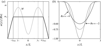
. This is sketched in figure 3(a). The corresponding new flow would be stable because all negative gradients
 $\text{d}m/\text{d}y$
would have disappeared for
 $y<0$
and all positive gradients for
 $y>0$
.
(a) Schematic of the predicted momentum distribution. The thin curve is the initial
 $m$
-distribution
 $M(y)$
for an unstable Gaussian jet (
 $\mathit{Ro}<-1/2$
). Instability commences in the two regions, on the left
 $y\in [\,y_{-},\,0]$
which connects to the region on the right with
 $y\in [0,\,y_{+}]$
as also indicated in figure 2(b). The values of
 $y_{\pm }$
are a function of the Rossby number according to (3.7). The left instability region is associated with
 $\text{d}M/\text{d}y<0$
and right instability region with
 $\text{d}M/\text{d}y>0$
so that
 $y\text{d}M/\text{d}y>0$
or equivalently
 ${\it\Phi}<0$
. The outer limits
 $\{y_{-},y_{+}\}$
are indicated with the thin dashed vertical lines. The prediction for the equilibrated flow is indicated with the thick solid curve. It has constant
 $m=m_{c}<0$
between
 $y=\pm y_{mix}$
indicated by the thin solid vertical lines. Equation (3.9) determines how non-dimensional
 $m_{c}$
and
 $y_{mix}$
vary with the Rossby number when
 $\mathit{Ro}<-1/2$
(see text). (b) The initial Gaussian jet (thin line) and the predicted final flows according to (3.10) for
 $\mathit{Ro}=-2$
and
 $\mathit{Ro}=-4$
. In each case the amplitudes have been scaled with
 $|\mathit{Ro}|$
to facilitate comparison. For
 $\mathit{Ro}=-2$
the maximum amplitude (at
 $y=0$
) has decreased 25 %, for
 $\mathit{Ro}=-4$
the decrease is 40 %.

If this is indeed what happens, then
 $y_{mix}$
is determined by the condition
 $$\begin{eqnarray}\int _{-y_{mix}}^{+y_{mix}}\{|\mathit{Ro}|\exp (-y^{2})+y^{2}/2\}\text{d}y=\int _{-y_{mix}}^{+y_{mix}}\{|\mathit{Ro}|\exp (-y_{mix}^{2})+y_{mix}^{2}/2\}\text{d}y,\end{eqnarray}$$
which yields the transcendental relation between
 $y_{mix}$
and
 $|\mathit{Ro}|$
 $$\begin{eqnarray}\int _{0}^{+y_{mix}}|\mathit{Ro}|\exp (-y^{2})\text{d}y=y_{mix}|\mathit{Ro}|\exp (-y_{mix}^{2})+y_{mix}^{3}/3,\end{eqnarray}$$
which is easily solved numerically. Knowing
 $y_{mix}$
as a function of
 $|\mathit{Ro}|$
we also know
 $m_{c}(|\mathit{Ro}|)$
, and we can predict that the adjusted absolute momentum and velocity profile non-dimensionally are
 $$\begin{eqnarray}\left.\begin{array}{@{}lll@{}}m=m_{c}, & u=m_{c}+y^{2}/2, & y\in [-y_{mix},+y_{mix}],\\ m=M(y), & u=U(y), & y\notin [-y_{mix},+y_{mix}],\end{array}\right\}\end{eqnarray}$$
with non-dimensional
 $U$
as in (3.2). Note that for all negative
 $\mathit{Ro}$
, according to (3.2), the initial
 $m(y)<0$
for all
 $y$
and that for increasing
 $|\mathit{Ro}|$
the value of the predicted
 $m_{c}$
gets ever more negative while the predicted mixing region
 $[-y_{mix},+y_{mix}]$
gets ever broader. This is illustrated in figure 3(b) where we plot the velocity profiles we expect to find after equilibration of the inertial instability for
 $\mathit{Ro}=-2$
and
 $\mathit{Ro}=-4$
.
3.2. Numerical simulations
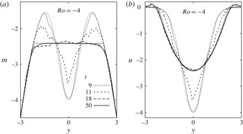
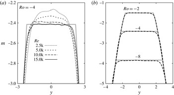
We now demonstrate that numerical simulations confirm the predictions for the equilibration of the westward flowing Gaussian jet at the equator. In figure 4, we show the evolution of the vertically averaged profiles of
 $m$
and
 $u$
as the inertial instability unfolds and equilibrates. As discussed in § 2, the vertical wavelength of the inertial instability vanishes at infinite Reynolds number. All of the simulations that we present will have a finite Reynolds number, which we define in the Gaussian case as
 $\mathit{Re}=|U_{0}|L/{\it\nu}$
. With viscosity, the most unstable mode has a finite vertical wavelength. The resolution that we use in all the simulations presented here will be sufficient to resolve the most unstable mode and also, as best as we can, all of the significant smaller scale motions that are generated nonlinearly. In the simulation used to prepare figure 4,
 $\mathit{Re}=15$
k (i.e. 15 000). The Rossby number is as defined in (3.2), and in this simulation
 $\mathit{Ro}=-4$
.
Profiles of vertically averages of (a) absolute momentum
 $m$
and (b) zonal velocity
 $u$
for a westward flowing Gaussian zonal jet centred on the equator. Here
 $\mathit{Ro}=-4$
and
 $\mathit{Re}=|U_{0}|L/{\it\nu}=15$
k. The full computational domain for this simulation is such that
 $z\in [0,4{\rm\pi}]$
and
 $y\in [-6,+6]$
on a grid of
 $513\times 513$
points. Here we are showing only the
 $y\in [-3,+3]$
portions of the profiles. Thick grey lines indicate the prediction. Along the axis
 $y$
is non-dimensionalized with the length scale
 $L$
. Time has been non-dimensionalized with the time scale
 $({\it\beta}L)^{-1}$
.

In figure 4(a), we see that the profile of vertically averaged momentum changes rapidly from the initial condition (thin grey line) to a nearly equilibrated state at non-dimensional time
 $t=18$
. The predicted equilibrium is shown as a thick grey line. After
 $t=18$
, the evolution is much slower, with the profile becoming smoother as seen at
 $t=50$
. The subsequent evolution is primarily slow viscous diffusion of momentum. The
 $m$
-profile evolves toward the homogeneous mixed state in the mixing region as predicted by our mixing scheme. The corresponding evolution of the profile of vertically averaged velocity
 $u$
is shown in figure 4(b). The profile rapidly evolves toward the predicted profile. As predicted, the maximum velocity of the jet is reduced in value by about a factor of a half during the equilibration. The match between the profile at
 $t=50$
(thin solid black curve) and the prediction (thick grey curve) is excellent for most of the jet. In the region just outside of the predicted mixing region, there is a small overshoot at
 $t=50$
in which a small amount of eastward flow is found. This has also been noted before in examples of flow on the
 $f$
-plane (see Kloosterziel et al.
Reference Kloosterziel, Orlandi and Carnevale2007b
).
Figure 5 shows how the results of equilibration vary with
 $\mathit{Re}$
and
 $\mathit{Ro}$
. Figure 5(a) confirms that, as in our previous work with flows on the
 $f$
-plane, the match between the vertically averaged profile of
 $m$
and the prediction improves with increasing
 $\mathit{Re}$
. Here the view is ‘zoomed-in’ relative to that shown in figure 4(a), and we see that the curve for
 $m$
at
 $t=50$
and
 $\mathit{Re}=15$
k is not perfectly flat. The irregularities are the result of perturbation vortices (see below) that have not yet dissipated. Figure 5(b) shows that equilibration occurs similarly over a wide range of unstable
 $\mathit{Ro}$
.
Effects of variation of (a)
 $\mathit{Re}$
and (b)
 $\mathit{Ro}$
on the equilibration of inertial instability of the Gaussian jet. All of the simulation results are taken at
 $t=50$
. The size of the computational domain and the resolution are as described in the caption of figure 4. Thick grey lines indicate the predictions.

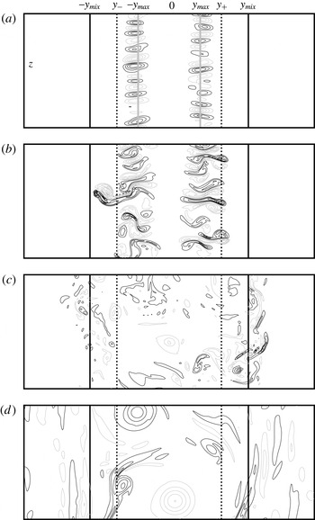
The vortex dynamics of the equilibration process for the Gaussian zonal jet on the equator in the standard
 ${\it\beta}$
-plane model is illustrated in figure 6. Only the along-stream component of the vorticity
 ${\it\omega}_{x}=\partial w/\partial y-\partial v/\partial z$
is shown since it is the growth of this component that characterizes the inertial instability, that is, the inertial instability is characterized by secondary overturning motions with their axis aligned with the flow direction as sketched in figure 1(a).
Contour plots of
 ${\it\omega}_{x}$
from a simulation of the Gaussian jet with
 $\mathit{Ro}=-4$
and
 $\mathit{Re}=15$
k at non-dimensional times (a)
 $t=7.5$
, (b) 10, (c) 20, (d) 50. The along-flow component of the vorticity is
 ${\it\omega}_{x}=\partial w/\partial y-\partial v/\partial z$
with
 $v,w$
the velocity components in the
 $y$
and
 $z$
direction, respectively. The initial instability region, is bounded by the vertical dashed lines, at
 $y_{-}$
and
 $y_{+}$
. The predicted outer limits of the inertial instability equilibration range,
 $y=-y_{mix}$
and
 $y=+y_{mix}$
, are indicated by the vertical solid black lines. Positive/negative contours are drawn as black/grey lines. The zero contour level is not drawn. The contour increments are (a) 0.5, (b) 4.0, (c) 4.0, (d) 1. In (a), the vertical solid grey lines indicate the initial positions
 $\pm y_{max}$
of maximum growth rate according to linear theory. These are also indicated in figure 2(b). Only a portion (
 $y\in [-4,+4]$
,
 $z\in [0,{\rm\pi}]$
) of the full computational domain (
 $y\in [-6,+6]$
,
 $z\in [0,4{\rm\pi}]$
) is shown.

In the earliest phase of the evolution (see figure 6
a,
 $t=7.5$
) two vertical columns of counter-rotating vortices form in the
 ${\it\omega}_{x}$
-field. Each column is centred on the position of maximum growth rate
 $\pm y_{max}$
as discussed above and marked here by a thick grey vertical straight line. The columns or stacks of vortices result from the linear phase of the instability. The shape and distribution of the vortices are somewhat irregular due to the nature of the initial random perturbation that we have used to initiate the evolution. As an aid to the discussion, we also include vertical black dashed lines marking the limits of the linear instability region (
 $y_{-},y_{+}$
) and vertical solid black lines marking the limits of the predicted mixing range at
 $y=\pm y_{mix}$
(see figure 2
b).
As the vortices grow in strength, they begin to interact nonlinearly. They pair with neighbours, both above and below, forming dipolar ‘heads’ and ‘tails’. As these dipolar ‘heads’ and ‘tails’ develop, the vorticity in them tends to roll up. Consider figure 6(b) (
 $t=10$
). In the region of positive
 $y$
, what we are calling ‘dipolar heads’ have a positive vortex on the top and a negative vortex on the bottom. With this configuration, self-advection transports the dipolar head in the positive (northward)
 $y$
direction. Hence, these dipoles are on a trajectory to leave the region of linear instability. In the negative
 $y$
region the dipolar heads are those dipoles that form with negative vorticity on top and positive on the bottom. Hence, for them, the sense of self-advection is in the negative (southward)
 $y$
direction and thus they are also on a trajectory to exit the linear instability region. By
 $t=10$
, we see that some of the dipolar heads are crossing the boundaries of the linear instability region and one has already escaped. By this process, the perturbation is not confined to the linearly unstable region and mixing can occur well beyond that region. Also note that the vortices have formed dipolar tails and that these are oriented to propagate toward the equator at
 $y=0$
. Thus this mechanism of dipolar ‘head’ and ‘tail’ formation allows the instability to propagate beyond the linear instability region and to mix vigorously even within it.
By
 $t=20$
(figure 6
c), the strength of the vortical motions is decaying. The dipolar ‘heads’ have travelled to and beyond the predicted limits of the mixing range. As the dipoles approach these limits, they tend to be deflected as is already evident for one dipolar ‘head’ seen on the left in figure 6(b). In figure 6(c), we see that some of the dipolar ‘heads’ have left the predicted mixing region and have actually turned around and are oriented so as to return toward that region. There is also what we might call ‘debris’ from the destruction of the dipolar heads that have left, or tried to leave, the mixing region. By
 $t=50$
(figure 6
d), the
 ${\it\omega}_{x}$
field has decayed significantly from its peak strength, although there are some remaining regions of activity. Outside the mixing region in figure 6(d) there is some evidence of inertial wave radiation.
To conclude this section we note that the domain-integrated potential vorticity or absolute vorticity, i.e.
 $\int \!Q(y)\text{d}y$
, is conserved. For the initial flow
 $Q=-\text{d}M/\text{d}y$
with
 $M(y)$
the momentum distribution, while for the predicted equilibrated flow the potential vorticity is
 $q=-\text{d}m/\text{d}y$
, with
 $m$
the momentum distribution which has
 $m=m_{c}$
between
 $y=-y_{mix}$
and
 $y=+y_{mix}$
. Hence
 $$\begin{eqnarray}\int _{-y_{mix}}^{+y_{mix}}Q(y)\text{d}y=-[M(y_{mix})-M(-y_{mix})]=-\int _{-y_{mix}}^{+y_{mix}}\frac{\text{d}m}{\text{d}y}\text{d}y=\int _{-y_{mix}}^{+y_{mix}}q(y)\text{d}y\end{eqnarray}$$
because in the prediction the level curve
 $m=m_{c}$
connects with
 $M(y)$
at
 $y=\pm y_{mix}$
(see figure 3
a). More generally, any
 $m(y)$
which connects with
 $M(y)$
at some
 $y=y_{l}$
and
 $y=y_{h}$
implies potential vorticity conservation but only certain choices imply momentum conservation.
4. Uniform shear flow
The linear stability properties of uniform shear flows
 $U(y)={\it\Lambda}y$
on the equatorial
 ${\it\beta}$
-plane was first studied by Dunkerton (Reference Dunkerton1981) and in several papers thereafter by that author and others, with extensions including double diffusion effects (Prandtl number
 $\mathit{Pr}\neq 1$
) and non-symmetric disturbances (see references in Griffiths Reference Griffiths2008). In two earlier papers Griffiths (Reference Griffiths2003a
,Reference Griffiths
b
) included the effect of uniform stratification (constant buoyancy parameter
 $N$
) but he used the hydrostatic approximation and just vertical diffusion of momentum. As a consequence the problem could be characterized by a single non-dimensional parameter
 ${\it\epsilon}=(2{\it\nu}N^{2}{\it\beta}^{2}/{\it\Lambda}^{5})^{1/3}$
. This makes it difficult to say what the Reynolds number was in his numerical simulations. Nonetheless, in the study of the uniform shear flow by Griffiths (Reference Griffiths2003b
), the resolution was high enough (
 $256\times 256$
grid points) to clearly see the instability develop, and as it proceeded the instability homogenized
 $fQ$
. The initial region of instability where
 $fQ={\it\Phi}<0$
disappeared and over some range a new flow emerged near neutral stability with
 $Q\approx 0$
.
In this section, we determine this range and determine the mixed
 $m_{c}$
that emerges with simulations using resolutions varying between
 $1537\times 1537$
and
 $2049\times 2049$
grid points. First, however, note that for
 $U(y)={\it\Lambda}y$
, we have dimensionally
 $$\begin{eqnarray}\left.\begin{array}{@{}c@{}}{\it\Phi}=fQ={\it\beta}y({\it\beta}y-\text{d}U/\text{d}y)=-{\it\beta}y\text{d}M/\text{d}y={\it\beta}y({\it\beta}y-{\it\Lambda}),\\ M={\it\Lambda}y-{\it\beta}y^{2}/2.\end{array}\right\}\end{eqnarray}$$
For definiteness we just consider positive shear
 ${\it\Lambda}>0$
. Then the instability range where
 ${\it\Phi}<0$
is between
 $y=y_{-}=0$
and
 $y=y_{+}={\it\Lambda}/{\it\beta}$
.
The length scale
 $L={\it\Lambda}/{\it\beta}$
is used to non-dimensionalize latitude
 $y$
and depth
 $z$
, and, as in the previous section, a time scale
 $T=1/{\it\beta}L=1/{\it\Lambda}$
is used to non-dimensionalize time
 $t$
, and a velocity scale
 $L/T={\it\Lambda}^{2}/{\it\beta}$
to non-dimensionalize momentum
 $m$
and zonal velocity
 $u$
. The non-dimensional Rayleigh discriminant is
 $\tilde{{\it\Phi}}={\it\Phi}/{\it\Lambda}^{2}$
. With that understood, non-dimensionally
 $$\begin{eqnarray}\left.\begin{array}{@{}l@{}}M=y-y^{2}/2,\quad U=y,\\ \tilde{{\it\Phi}}=y(y-1)=-y\text{d}M/\text{d}y.\end{array}\right\}\end{eqnarray}$$
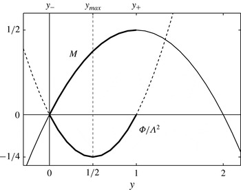
Instability occurs between non-dimensional
 $y=y_{-}=0$
and
 $y=y_{+}=1$
. This is illustrated in figure 7. Both
 $\tilde{{\it\Phi}}$
and
 $M$
are parabolas with (non-dimensionally) a negative minimum
 $\tilde{{\it\Phi}}_{m}=-1/4$
at
 $y=y_{max}=1/2$
and a maximum
 $M=1/2$
at
 $y=1$
( for negative shear
 ${\it\Lambda}<0$
, see caption of figure 7). Here
 $|{\it\Phi}|_{m}=\max \{-{\it\Phi}\}={\it\Lambda}^{2}/4$
and if exponential growth is assumed, i.e.
 $\exp ({\it\gamma}t)$
, the growth rate
 ${\it\gamma}<|{\it\Phi}|_{m}^{1/2}=|{\it\Lambda}|/2$
.
Non-dimensional
 $\tilde{{\it\Phi}}={\it\Phi}/{\it\Lambda}^{2}$
and
 $M=M/({\it\Lambda}^{2}/{\it\beta})$
as a function of non-dimensional
 $y=y/L$
with
 $L={\it\Lambda}/{\it\beta}$
for positive shear
 ${\it\Lambda}>0$
. The position of the fastest growth is expected at
 $y_{max}=1/2$
. The instability region is between
 $y=y_{-}=0$
and
 $y=y_{+}=1$
. For negative shear
 ${\it\Lambda}<0$
, using the length scale
 $L=|{\it\Lambda}|/{\it\beta}$
one would get
 $M=-y-y^{2}/2$
,
 ${\it\Phi}=y(y+1)$
instead of (4.2) with instability between
 $y=y_{-}=-1$
and
 $y=y_{+}=0$
and maximal growth at
 $y=y_{max}=-1/2$
. For negative shear the two parabolas (
 $M$
and
 ${\it\Phi}$
) are simply shifted one non-dimensional unit to the left and all is simply a reflection of what is seen here across the equator at
 $y=0$
.

Instability is expected to manifest itself initially as overturning motions centred about
 $y=y_{max}$
, just as in one of the two instability regions for the unstable Gaussian jet, i.e. as either the pattern on the left or right of figure 6(a).
4.1. Prediction?
For the uniform shear flow we face a problem: the initial
 $m$
-distribution
 $m=M(y)$
, as seen in figure 7, has a single maximum with no adjacent minima. If again we assume that the instability sets the
 $m$
-distribution to some constant
 $m=m_{c}$
over some
 $y$
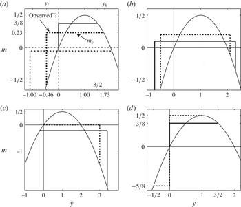
-range, there is no obvious answer. Various equally plausible possible equilibria are sketched in figure 8. All satisfy the constraint of total absolute momentum conservation.
Examples of possible momentum distributions of equilibrated flows for positive shear
 ${\it\Lambda}>0$
. In each panel the initial unstable
 $m$
-distribution is the parabola (thin solid line) with non-dimensional
 $m=M=y-y^{2}/2$
as in (4.2). Instability range is between non-dimensional
 $y=0$
and
 $y=1$
(see figure 7). (a) ‘Observed’ case (see text) with
 $m_{c}=0.232$
and
 $y_{l}=-0.464$
,
 $y_{h}=1.732$
(dashed), special case
 $m_{c}=3/8$
and
 $y_{l}=0$
,
 $y_{h}=3/2$
(thick solid) and a case with
 $m_{c}<0$
(dot-dashed). In each case (4.3) is satisfied. There is a positive jump at
 $y=y_{l}$
and continuity at
 $y=y_{h}$
with
 $m_{c}=M(y_{h})$
. The equality
 $2y_{h}+y_{l}=3$
is satisfied. (b) Two examples (thick dashed and thick solid) with
 $m=m_{c}$
between
 $y=y_{l}<0$
and
 $y=y_{h}>0$
and a positive jump at
 $y=y_{l}$
and negative jump at
 $y=y_{h}$
. (c) Continuous at
 $y=y_{l}\leqslant 0$
and negative jump at
 $y=y_{h}>0$
. Case
 $m_{c}=0$
,
 $y_{l}=0$
,
 $y_{h}=3$
is the thick dashed line. (d) Example (thick dashed line) with an internal jump at
 $y=0$
(equator) and two different
 $m_{c}$
-levels. Case
 $m_{c}=3/8$
and
 $y_{l}=0$
,
 $y_{h}=3/2$
(thick solid line) also shown in (a). For negative shear
 ${\it\Lambda}<0$
all these graphs have to flipped about the
 $y=0$
axis (see remarks in the caption of figure 7).

First note that always at least one discontinuity (a ‘jump’) in the equilibrated
 $m$
-profile would be required as in figure 8(a), where we show three possibilities that conserve
 $m$
. The jump is ‘positive’ ( from lower
 $m$
to higher
 $m$
) on the left in the region
 $y\leqslant 0$
in each case at
 $y=y_{l}$
. A positive jump in the region
 $y>0$
would correspond to an unstable situation with
 ${\it\Phi}=-y\text{d}m/\text{d}y<0$
since
 $\text{d}m/\text{d}y=+{\it\delta}(y)$
. On the right, the adjusted profile connects at
 $y=y_{h}$
with the initial
 $m$
-profile with the condition that
 $$\begin{eqnarray}\int _{y_{l}}^{y_{h}}(M(y)-m_{c})\text{d}y=0,\end{eqnarray}$$
and in this case
 $m_{c}=M(y_{h})$
. We marked as ‘observed’ the case (dashed) with
 $m_{c}=0.232$
and
 $y_{l}=-0.464$
,
 $y_{h}=1.732$
which we will discuss further below. Also shown is the special case (solid)
 $m_{c}=3/8$
and
 $y_{l}=0$
,
 $y_{h}=3/2$
. Amongst the three possibilities shown in figure 8(a), this case has the smallest range over which
 $m=m_{c}$
with width
 $y_{h}-y_{l}=3/2$
.
In figure 8(b), we show two cases with a positive jump at
 $y=y_{l}<0$
and a negative jump at
 $y=y_{h}>0$
which also satisfy (4.3). In figure 8(c), we show the opposite of the scenario shown in figure 8(a), i.e. an adjusted profile which is continuous in
 $m$
at
 $y=y_{l}\leqslant 0$
and a negative jump at
 $y=y_{h}>0$
. The particular case with
 $m_{c}=0$
and
 $y_{l}=0$
,
 $y_{h}=3$
is the dashed line. Finally, in figure 8(d), we show yet another possibility with an ‘internal’ jump at
 $y=0$
but continuous at
 $y=y_{l}\leqslant 0$
and
 $y=y_{h}>0$
. The particular case with
 $m=m_{c}=-5/8$
between
 $y_{l}=-1/2$
and
 $y=0$
and
 $m=m_{c}=1/2$
between
 $y=0$
and
 $y_{h}=1$
is shown as the dashed line. This has the same ‘width’ (
 $y_{h}-y_{l}=3/2$
) as the other case shown in figure 8(d) (thick solid line with a jump at
 $y_{l}=0$
and continuous at
 $y_{h}=3/2$
), which is also shown in figure 8(a).
All scenarios sketched in figure 8(a–c) imply conservation of total potential vorticity. Without going into details, it suffices to point out that the jumps can be represented using the Heaviside stepfunction multiplied by the appropriate jump amplitude. This means that in the
 $q$
-distribution there will be
 ${\it\delta}$
-functions at the jump locations. It is easily verified that this implies that
 $\int \!q(y)\text{d}y=\int \!Q(y)\text{d}y$
. Hence potential vorticity conservation does not provide an additional constraint with which a particular final equilibrium is singled out. In the same way it can also be shown that the dashed-line solution with the ‘internal’ jump in figure 8(d) also implies potential vorticity conservation. However, that solution can be ruled out because it has more energy than the initial state. In all cases, the final equilibrated state must have less energy than the initial state. Even taking into consideration this energy constraint, all examples shown in figure 8(a–c) are viable candidates. What nature will choose is thus not clear at all. The numerical simulations will provide the answer.
4.2. Numerical simulations
For the numerical simulations, it remains only to define the Reynolds number for the flow. Using the length scale
 $L={\it\Lambda}/{\it\beta}$
and time scale
 $T=1/{\it\Lambda}$
, the non-dimensional reciprocal of
 ${\it\nu}$
gives us the Reynolds number
 $\mathit{Re}={\it\Lambda}^{3}/({\it\beta}^{2}{\it\nu})$
for this flow.
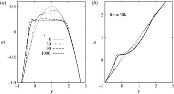
The evolution of the profiles of vertically averaged absolute momentum
 $m$
and zonal velocity
 $u$
for the uniform shear flow is shown in figure 9. Once the instability begins,
 $m(y)$
goes through a rapid change, resulting by non-dimensional time
 $t=90$
in a relatively flat mixed region (figure 9
a). On the northern (positive
 $y$
) end of this mixed region, the flat portion of
 $m(y)$
joins the initial condition without a jump. On the southern side, however, the mixed region joins the initial condition by a relatively steep jump at approximately
 $y=-1/2$
. As time proceeds, the mixed region tends to get smoother and flatter, while the slope of the jump tends to become shallower. This shallowing of the jump is a result of long-term viscous diffusion.
Profiles of vertically averaged (a) absolute momentum
 $m$
and (b) zonal velocity
 $u$
for the uniform shear flow at the equator. The full computational domain for this simulation is
 $y\in [-4,+4]$
and
 $z\in [0,2{\rm\pi}]$
on a grid of
 $1537\times 1537$
points. Here we show only the
 $y\in [-1,+3]$
portion of the profiles. The Reynolds number of the flow is
 $\mathit{Re}={\it\Lambda}^{3}/{\it\beta}^{2}{\it\nu}=50$
k.

The evolution of
 $u(y)$
is illustrated in figure 9(b). As the
 $u(y)$
profile evolves, a step-like bump forms on the profile around non-dimensional
 $y\approx -1/2$
. The steepness of the positive (upward) slope of this bump increases rapidly between
 $t=30$
and
 $t=90$
. The steepness is greatest at
 $t=90$
, and then it slowly and continually becomes shallower from
 $t=90$
to the end of the simulation at
 $t=1000$
.
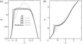
The effect of varying
 $\mathit{Re}$
on the equilibrium achieved after inertial instability is illustrated in figure 10. The curves drawn for various
 $\mathit{Re}$
in each panel of the figure correspond to non-dimensional time
 $t=200$
when the inertial instability is essentially equilibrated and slow viscous diffusion has not yet severely affected the profiles. Figure 10(a) demonstrates that as
 $\mathit{Re}$
increases,
 $m(y)$
becomes flatter and smoother in the ‘mixed region’, the region extends farther in the negative
 $y$
direction, and the steepness of the jump near
 $y\approx -1/2$
increases. The corresponding curves for
 $u(y)$
are shown in figure 10(b). The bump on the profile between
 $y\approx -1$
and
 $y\approx 0$
becomes increasingly step-like, with the jump becoming steeper with increasing
 $\mathit{Re}$
. The sharp gradient in
 $u$
at
 $y\approx -1/2$
corresponds to a large negative value of the (non-dimensional) potential vorticity
 $q=y-\text{d}u/\text{d}y$
. This was also observed in the numerical simulations of Griffiths who added uniform stratification to the problem (see Griffiths Reference Griffiths2003b
).
Variation with
 $\mathit{Re}$
of profiles of vertically averaged (a) absolute momentum
 $m$
and (b) zonal velocity
 $u$
for the uniform shear flow at the equator. The curves all correspond to non-dimensional time
 $t=200$
by which the inertial instability has essentially equilibrated, but before viscous diffusion has had time to begin to smooth out the jump near
 $y\approx 0.5$
. The full computational domain is
 $y\in [-4,+4]$
and
 $z\in [0,2{\rm\pi}]$
on a grid of
 $2049\times 2049$
points. Only the
 $y\in [-1,+3]$
section of the computational domain is shown. The thick grey line in (a) is the prediction (4.4) with
 $m_{c}=0.232$
and
 $y_{l}=-0.464$
,
 $y_{h}=1.732$
, also marked as ‘observed’ in figure 8(a). The thin grey line in each plot corresponds to the initial condition. The Reynolds number is defined as
 $\mathit{Re}={\it\Lambda}^{3}/{\it\beta}^{2}{\it\nu}$
.

Based on these results and experience with equilibration on the
 $f$
-plane (see Kloosterziel et al.
Reference Kloosterziel, Carnevale and Orlandi2007a
,Reference Kloosterziel, Orlandi and Carnevale
b
; Carnevale et al.
Reference Carnevale, Kloosterziel, Orlandi and van Sommeren2011, Reference Carnevale, Kloosterziel and Orlandi2013), we hypothesize that in the limit of infinite
 $\mathit{Re}$
the equilibrium profile of
 $m$
would be perfectly flat in the mixing region and there would be a jump discontinuity on the southern side of the mixing region at
 $y\approx -1/2$
. This would then correspond to one of the examples from figure 8(a). If
 $m_{c}$
is the level of
 $m$
in the mixing region and
 $y_{l}$
the location of the jump, then we hypothesis that the equilibrium profile would be
 $$\begin{eqnarray}\left.\begin{array}{@{}lll@{}}m=m_{c}, & u=m_{c}+y^{2}/2, & y\in [\,y_{l},y_{h}],\\ m=M(y)=y-y^{2}/2, & u=U(y)=y, & y\notin [\,y_{l},+y_{h}].\end{array}\right\}\end{eqnarray}$$
Assuming conservation of total absolute momentum according to (4.3), we find a cubic equation relating
 $y_{l}$
to
 $y_{h}$
for any given
 $m_{c}$
. Using the assumed continuity at
 $y=y_{h}$
so that
 $m_{c}=M(y_{h})$
this yields an exact relation:
 $2y_{h}+y_{l}=3$
. Based on the observed level
 $m_{c}\approx 0.232$
, from
 $M(y_{h})=m_{c}$
we obtain
 $y_{l}=-0.464$
and
 $y_{h}=1.732$
which agrees with the observed location of the jump near
 $y\approx -1/2$
. We have already sketched this solution in figure 8(a). It is drawn as the thick grey line in figure 10(a). This is not the solution of the smallest possible mixing range, nor does it correspond to any possible extremization of energy loss. There is no simple principle that we have been able to determine that selects this particular solution, even restricting consideration to the class of possibilities shown in figure 8(a).
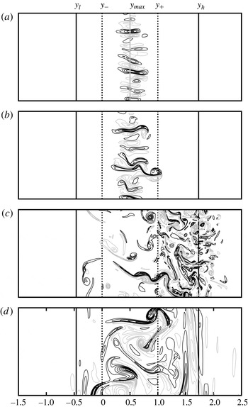
The vortex dynamics behind the instability and its equilibration in the uniform shear flow are illustrated in figure 11. The evolution is similar to what we have seen in the Gaussian case but for the difference that in the
 ${\it\omega}_{x}$
field just one vertical column of vortices of alternating sign forms at the position of maximum growth as predicted by linear theory (figure 11
a). Each vortex pairs with its two neighbours to form dipolar heads/tails propagating in the negative/positive
 $y$
direction (figure 11
b). These dipolar structures propagate beyond the region of linear instability and fill out a region where the absolute momentum becomes well mixed (figure 11
c). As equilibration nears completion, there remain some relatively weak, long lived, vortex structures in the mixing region and some weak inertial waves beyond (figure 11
d). Clearly, the evolution seen in figure 11 is not symmetric as in the Gaussian jet case (see figure 6): we have only one region of instability from which intense activity emerges on the northern (positive
 $y$
) side of the mixing region, away from the equator at
 $y=0$
, while far less is seen to the south of the equator where the jump develops.
Contour plots of
 ${\it\omega}_{x}$
from a simulation of the uniform shear flow with
 $\mathit{Re}=50$
k at non-dimensional times (a)
 $t=18$
, (b)
 $t=22$
, (c)
 $t=50$
(d)
 $t=1000$
. The initial instability region, is bounded by the vertical dashed lines, at
 $y_{-}=0$
(the equator) and
 $y_{+}=1$
. The final limits of the inertial instability equilibration range,
 $y_{l}\approx -0.46$
and
 $y_{h}\approx +1.73$
, are indicated by the vertical solid black lines. Only a portion (
 $y\in [-1.5,2.5]$
,
 $z\in [0,{\rm\pi}/2]$
) of the full computational domain (
 $y\in [-4,+4]$
,
 $z\in [0,2{\rm\pi}]$
) is shown. The computation is done on a grid of
 $1537\times 1537$
points. Positive/negative contours are drawn as black/grey lines. The zero contour level is not drawn. The contour increments are (a) 0.42, (b) 1.5, (c) 3.1, (d) 0.15. In (a), the vertical solid grey line indicates the initial position of maximum growth rate
 $y_{max}=1/2$
according to linear theory. The Reynolds number of the flow is
 $\mathit{Re}={\it\Lambda}^{3}/{\it\beta}^{2}{\it\nu}=50$
k.

5. East- and westward flowing jets off the equator
In § 3 we showed that the eastward flowing Gaussian jet is always stable when centred on the equator whereas the westward jet can be unstable but only when
 $\mathit{Ro}=U_{0}/{\it\beta}L^{2}<-1/2$
(remember a flow to the east has
 $U_{0}>0$
, to the west
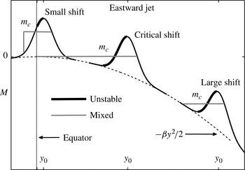
 $U_{0}<0$
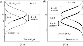
). But if the flow axis of the eastward jet is shifted to some small distance
 $y_{0}$
away from the equator there will be instability, even for very small Rossby numbers. This is illustrated in figure 12(a), where the thin Gaussian curve shows the stable eastward jet on the equator. If the axis is however at
 $y=y_{0}>0$
(north of the equator) there will be positive shear
 $\text{d}U/\text{d}y>0$
in the region between the equator at
 $y=0$
and
 $y=y_{0}$
. This implies that the Rayleigh discriminant
 ${\it\Phi}={\it\beta}y({\it\beta}y-\text{d}U/\text{d}y)<0$
between
 $y=0$
and some
 $y<y_{0}$
(indicated by the thick line in figure 12
a). We call a shift ‘large’ when the jet has a negligible velocity amplitude at the equator. Then
 $f={\it\beta}y$
is of one sign over the entire region occupied by the jet and stability/instability is only determined by the sign of
 $Q={\it\beta}y-\text{d}U/\text{d}y$
or
 $\text{d}M/\text{d}y(\equiv -Q)$
. Then essentially
 $f$
-plane dynamics is found. The transition between a large and a small shift occurs via a ‘critical’ shift. This special shift-value
 $y_{0}$
varies with the Rossby number
 $\mathit{Ro}$
. This will be further clarified below. Figure 13 illustrates the distinction we shall make between ‘small’, ‘critical’ and ‘large’.
Schematic showing a ‘top view’ of (a) an eastward Gaussian jet and (b) a westward Gaussian jet shifted northward with their axis a distance
 $y_{0}$
away from the equator. In (a) the shift
 $y_{0}$
is small so that finite positive shear is found between the equator (
 $y=0$
) and some location
 $y<y_{0}$
. This implies instability (thick line) where the positive shear
 $\text{d}U/\text{d}y>{\it\beta}y$
so that
 ${\it\Phi}<0$
. For small shifts the eastward jet is unstable for any Rossby number
 $\mathit{Ro}>0$
. In (b) the shift is small enough and
 $\mathit{Ro}$
sufficiently negative (
 $\mathit{Ro}<\mathit{Ro}_{cr}=-1/2$
) so that two regions of instability remain, one north of
 $y=y_{0}$
where
 $\text{d}U/\text{d}y>{\it\beta}y$
and one south of the equator (
 $y<0$
) where the negative shear
 $\text{d}U/\text{d}y<{\it\beta}y$
. In both regions
 ${\it\Phi}<0$
while separated by a stable region north of the equator. For the westward jet in (b) only the southern instability region remains if the magnitude of the Rossby numbers falls below some critical value. See text for more details.

Diagram showing a ‘side view’ of the absolute momentum distribution
 $M=U(y)-{\it\beta}y^{2}/2$
for the shifted eastward jet. Three possibilities are shown: a ‘small shift’ for which the equilibration can be predicted using the results from § 4 for the linear shear flow, a ‘critical shift’ which is a combination of
 $\mathit{Ro}$
and
 $y_{0}$
such that the predicted mixing range with constant
 $m=m_{c}$
extends to the equator, and a ‘large shift’ where equilibration is reached through mixing to some level
 $m_{c}$
as sketched in figure 1(b) for the
 $f$
-plane. To prepare this graph a fixed
 $\mathit{Ro}$
was used but variable
 $y_{0}$
. The critical case is only possible for
 $y_{0}>2.2$
. More details are provided in the text.

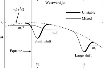
For the westward jet the situation is entirely different. This is sketched in figure 12(b). If
 $\mathit{Ro}<\mathit{Ro}_{cr}=-1/2$
and the jet is shifted, the two regions of instability (see figure 2
b) that were joined at the equator become separated. In figure 2(b) the thick Gaussian curve is the unstable jet on the equator with
 $\mathit{Ro}<-1.2$
. The shifted curve with two separate thick lines indicates that when
 $y_{0}>0$
there will be a region of instability south of the equator (
 $y<0$
) where the shear
 $\text{d}U/\text{d}y<0$
such that
 ${\it\Phi}={\it\beta}y({\it\beta}y-\text{d}U/\text{d}y)<0$
. Directly north of the equator a band of inertially stable flow emerges while beyond the peak at
 $y=y_{0}$
the other region of instability resides with sufficiently large positive shear
 $\text{d}U/\text{d}y>0$
so that
 ${\it\Phi}<0$
again. For a large northward shift, the shear south of the equator becomes negligible and only one region of instability is possible. Then, as for the eastward jet,
 $f$
-plane dynamics is recovered. But for small shifts of the westward Gaussian jet we encounter a case never studied before: there will be inertial instability in two nearby regions with unequal rates of growth. The secondary overturning motions seen above in figure 6(a,b) will grow faster on one side than on the other. Their nonlinear propagation into the region where the instability is growing at a smaller pace alters the flow there and no prediction of the outcome seems possible. This difficulty is sketched below in figure 16 on the left with the grey line marked ‘
 $m_{c}$
?’. For definiteness we will just discuss northward shifts (
 $y_{0}>0$
).
For either jet we simply take the velocity field
 $$\begin{eqnarray}U(y)=U_{0}\exp (-(y-y_{0})^{2}/L^{2})\end{eqnarray}$$
and the corresponding absolute momentum is therefore
 $$\begin{eqnarray}M=U_{0}\exp (-(y-y_{0})^{2}/L^{2})-{\it\beta}y^{2}/2.\end{eqnarray}$$
As in § 3 we non-dimensionalize
 $M$
and
 $U$
so that non-dimensionally
 $$\begin{eqnarray}M=\mathit{Ro}\exp (-(y-y_{0})^{2})-y^{2}/2,\quad U=\mathit{Ro}\exp (-(y-y_{0})^{2}),\quad \mathit{Ro}=U_{0}/{\it\beta}L^{2},\end{eqnarray}$$
and
 $y$
is non-dimensionalized with
 $L$
. The magnitude of the non-dimensional shift
 $y_{0}$
tells us how far we are away from the equator at
 $y=0$
. For example, a non-dimensional
 $y_{0}=3$
means the axis of the current is at a distance
 $3L$
. The condition for instability remains
 ${\it\Phi}<0$
or non-dimensionally
 $$\begin{eqnarray}y\frac{\text{d}M}{\text{d}y}=y\left(2(y-y_{0})\mathit{Ro}\exp (-(y-y_{0})^{2})+y\right)>0.\end{eqnarray}$$
This implies the use of the time scale
 $T=1/{\it\beta}L$
and velocity scale
 $L/T={\it\beta}L^{2}$
but for the numerical results presented below we found it more convenient to report times
 $t$
non-dimensionalized with the advective time scale
 $T=L/|U_{0}|$
and to define the Reynolds number as
 $\mathit{Re}=|U_{0}|L/{\it\nu}$
.
5.1. Eastward jet: small shift
In figure 12(a) we indicate what we mean by small: it is a combination of
 $y_{0}$
and
 $\mathit{Ro}$
such that the initial
 $M$
-distribution has
 $\text{d}M/\text{d}y>0$
in a range between the equator at
 $y=0$
and
 $y<y_{0}$
. This is also sketched in figure 13. The thick lines in both figures indicate this range. Locally the
 $M$
-distribution looks like a downward parabola, as for the uniform shear flow studied in § 4 (see figure 7). Hence the same ambiguity arises: how will the flow equilibrate? But since we now know how the linear shear flow adjusts, we can make a good guess. The answer is already sketched in figure 13: one can expect the development of a jump discontinuity south of the equator while momentum will be mixed to some constant level
 $m_{c}$
. A surprisingly good prediction for the mixing range and mixing level
 $m_{c}$
can be made using a linear shear matching procedure which is described in some detail in the appendix A.
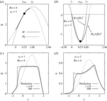
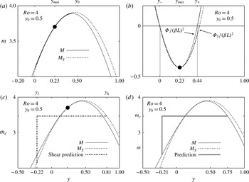
An example is shown in figure 14. This is for the eastward jet with
 $\mathit{Ro}=4$
and a shift
 $y_{0}=1$
. In the appendix A we illustrate the procedure for the same jet but with a smaller shift (
 $y_{0}=0.5$
, see figure 20). The idea is to approximate the initial momentum distribution
 $M$
around the position of maximal growth
 $y_{max}$
by
 $$\begin{eqnarray}M(y)\approx {\rm\Delta}M+Sy-By^{2}/2\equiv M_{S}.\end{eqnarray}$$
In figure 14(a) we show this approximation
 $M_{S}$
as a dotted line. It is obviously a downward parabola, just as the
 $M$
-profile of the uniform shear flow. At
 $y=y_{max}$
by construction we have
 $M_{S}=M$
and
 $M_{S}^{\prime }=M$
,
 $M_{S}^{\prime \prime }=M^{\prime \prime }$
(
 $M^{\prime }\equiv \text{d}M/\text{d}y,M^{\prime \prime }\equiv \text{d}^{2}M/\text{d}y^{2}$
). This means that also at
 $y_{max}$
the Rayleigh discriminant
 ${\it\Phi}_{S}\equiv -{\it\beta}y\text{d}M_{S}/\text{d}y={\it\Phi}$
. This is illustrated in figure 14(b). Even for this relatively large shift it is seen in the figure that
 ${\it\Phi}_{S}\approx {\it\Phi}$
over the entire instability range where
 ${\it\Phi}<0$
. In the appendix A it is explained why the flow that has initially a momentum distribution
 $M_{S}$
is expected to equilibrate with a mixing level
 $m_{c}={\rm\Delta}M+0.232(S^{2}/B)$
. The prediction only uses this predicted level and the assumption that just as for the linear shear flow a jump occurs south of the equator (
 $y=y_{l}<0$
), as in figure 8(a) (‘observed’) or for example figure 10(a), while at
 $y=y_{h}>0$
on the right-hand side of the mixing range
 $m_{c}=M$
. The location of the jump is then determined by momentum conservation, i.e. (4.3) is satisfied. The prediction is drawn as a thick grey curve in figure 14(c). It is seen that around
 $t=300$
when the flow has equilibrated, the vertically averaged momentum indeed matches the prediction remarkably well except near the jump position. In the simulation we used
 $\mathit{Re}=400$
k. Much higher
 $\mathit{Re}$
are expected to reveal a ‘sharpening’ of the jump, just as is seen in figure 10(a).
(a) Initial momentum
 $M$
(solid grey line) and the approximation
 $M_{S}$
(dotted line) for the eastward flowing jet with
 $\mathit{Ro}=4$
and shift
 $y_{0}=1$
. The approximation
 $M_{S}$
is given by (5.5) with non-dimensionalized
 ${\rm\Delta}M=1.11$
,
 $S=4.91$
,
 $B=4.58$
(see (A 5) in the appendix A). The location of fastest growth
 $y=y_{max}=0.53$
is indicated by a ●. The thick black part of
 $M$
indicates the instability region
 $y\in [0,0.88]$
. (b) Non-dimensionalized Rayleigh discriminant
 ${\it\Phi}$
(solid line) and the approximation
 ${\it\Phi}_{S}=-{\it\beta}y\text{d}M/\text{d}y$
(dotted line). The location of fastest growth
 $y=y_{max}=0.53$
is indicated by a ●. In (c) and (d) the prediction based on the linear shear dynamics (see appendix A) for the equilibrium
 $m$
and
 $u$
-field is shown as a thick grey curve. The black curve in (c) and (d) is the result at non-dimensional time
 $t=300$
of a numerical simulation of the equilibration of the eastward Gaussian jet with (c) absolute momentum
 $m$
vertically averaged and (d) velocity
 $u$
vertically averaged. At time
 $t=300$
the inertial instability has essentially equilibrated. The full computational domain is
 $y\in [-4,4]$
by
 $z\in [0,4{\rm\pi}]$
with 1025 grid points in each direction. Only a section of the
 $y$
-range is shown. The Reynolds number for the flow is
 $\mathit{Re}=|U_{0}|L/{\it\nu}=400$
k. In (d) the
 $u$
-field has been normalized with
 $\mathit{Ro}$
, i.e. we show
 $u/|\mathit{Ro}|$
so that the peak velocity at
 $t=0$
is
 $U(y_{0})/|\mathit{Ro}|=1$
.

The jump discontinuity that is seen to have formed in figure 14(c) was schematically indicated in the upper left part of figure 13. If we compare this with the results for the linear shear flow shown in figure 10(a), there is clearly little qualitative difference. But the adjusted velocity field seen in figure 14(d) for the Gaussian jet is obviously very different from the adjusted linear shear flow seen in figure 10(b). This indicates that for the adjustment of the inertial instability the finer details of the flow away from the initial instability region do not matter much. For example, in figure 14(d) the mixing has produced a profile which connects to the Gaussian profile to the right of the peak velocity (
 $y=y_{0}$
) where the flow is decreasing with distance. For the uniform shear flow in figure 10(b) the mixing has proceeded to the right to connect with the linearly increasing flow. But in both cases the initial momentum distributions and the Rayleigh discriminant in the region of instability and ultimate mixing region ‘look’ the same and this is all that matters.
5.2. Eastward jet: critical shift and large shift
From the diagram in figure 13 it should be clear that larger
 $\mathit{Ro}$
imply a larger ‘bump’ added to the downward parabola
 $-{\it\beta}y^{2}/2$
, the sum of which is the absolute momentum. It should also be clear that if the eastward jet with some fixed large
 $\mathit{Ro}$
is shifted to larger
 $y_{0}$
than just discussed, the mixing hypothesis (constant
 $m_{c}$
over some range and conservation of total absolute momentum) implies that for some
 $y_{0}$
the mixing range extends exactly to the equator but not beyond and no jumps south of the equator are expected. We call this the ‘critical shift’ although it is really a specific combination of
 $y_{0}$
and
 $\mathit{Ro}$
. Figure 13 shows an example. Experimentation with the mixing recipe reveals that the smallest shift for which the critical case occurs is
 $y_{0}\approx 2.2$
with
 $\mathit{Ro}\approx 1.98$
. For
 $y_{0}$
increasing monotonically above the value 2.2, the corresponding critical
 $\mathit{Ro}$
increases monotonically as well. For example, when
 $y_{0}=5$
the critical
 $\mathit{Ro}$
is
 $\mathit{Ro}=20.6$
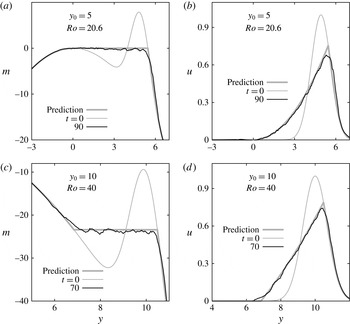
. The results of numerical simulation for this particular critical combination of
 $y_{0}$
and
 $\mathit{Ro}$
are shown in figure 15(a,b). Figure 15(a) shows that the inertial instability has mixed the momentum between the equator and a position to the right of the peak of the jet, as seen in figure 15(b). The agreement with our prediction (thick grey lines) is excellent. This example is representative for all possible critical cases with
 $y_{0}>2.2$
.
Plots of the vertically averaged absolute momentum
 $m(y)$
and
 $u(y)$
showing the initial (thin grey curve) conditions and the state after a time sufficient to allow nearly complete absolute momentum mixing (solid black curve), for the eastward flowing Gaussian initial jet on the
 ${\it\beta}$
-plane with: (a) and (b) a ‘critical shift’ example (see text) with
 $y_{0}=5$
and
 $\mathit{Ro}=20.6$
, (c) and (d) a ‘large shift’ example with
 $y_{0}=10$
and
 $\mathit{Ro}=40$
. In each panel the thick grey curve is the prediction based on our momentum mixing scheme with no discontinuities. For the critical case the mixed level in (a) is
 $m_{c}\approx 0$
. At time
 $t=90$
(a,b) and
 $t=70$
(c,d) the inertial instability has equilibrated. The full computational domain for (a) and (b) is
 $y\in [-3,9]$
by
 $z\in [0,4{\rm\pi}]$
with 1025 grid points in each direction. For (c) and (d) the
 $y$
-range is
 $y\in [2,14]$
. In all panels only a section of the
 $y$
-range is shown. The Reynolds number is
 $\mathit{Re}=50$
k. In (b) and (d) we show
 $u/|\mathit{Ro}|$
so that the peak velocity at
 $t=0$
is
 $U(y_{0})/|\mathit{Ro}|=1$
.

What we call ‘large’ next is somewhat arbitrary, but simply put: it is a combination of
 $y_{0}$
and
 $\mathit{Ro}$
so that the mixing does not reach the equator and no jumps are expected. One can see from figure 15(a) that if
 $\mathit{Ro}$
is slightly lowered from
 $\mathit{Ro}=20.6$
, the peak amplitude around
 $y_{0}=5$
in the initial momentum distribution (thin grey line) becomes a bit lower while barely affecting the depth of the ‘valley’ around
 $y=3$
because of the rapid fall-off of the Gaussian jet amplitude with distance from
 $y_{0}$
. Momentum can then be conserved by mixing between some
 $y=y_{l}>0$
and a position
 $y_{h}>y_{0}$
with an
 $m_{c}$
lower than in figure 15(a) so that (2.7) is satisfied. Instead of showing that, we show in figure 15(c,d) a case with
 $y_{0}=10$
and large
 $\mathit{Ro}=40$
. It is seen again that the agreement between the numerical results and the prediction is very good. This case was also sketched in figure 13. One may find this an extremely high Rossby number, but it is really a matter of definitions. Dimensionally
 $y_{0}=10$
corresponds to a distance
 $10L$
with
 $L$
the width of the Gaussian jet. The Coriolis parameter at
 $y_{0}$
is
 $f_{0}={\it\beta}y_{0}$
. If instead of
 $\mathit{Ro}=U_{0}/{\it\beta}L^{2}$
we choose
 $\mathit{Ro}=\mathit{Ro}_{f_{0}}=U_{0}/f_{0}L$
then with the shift
 $y_{0}=10L$
we would have had
 $\mathit{Ro}_{f_{0}}=4$
.
The reason for showing the example seen in figure 15(c,d) and not a more ‘reasonable’ one, is twofold. First, because although all in this study is formulated in the context of equatorial
 ${\it\beta}$
-plane dynamics, things quickly start to look like mid-latitude
 $f$
-plane dynamics. Figure 1(b) for example used the absolute momentum on the
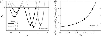
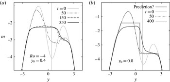
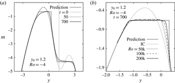
 $f$
-plane, i.e.
 $M=U(y)-f_{0}y$
(with
 $U$
also a Gaussian jet) but it is not unlike figure 15(c). Secondly, if figure 15(a) is compared with 15(c), one sees very different initial momentum distributions. But the mixing through inertial instability leads to adjusted, inertially stable flows that differ very little, as comparison of panel (b) with panel (d) of figure 15 reveals. Note that although ‘
 $f$
-plane-like’ adjustments are observed, the length scale
 $L$
can be anything, say a mere 10 km. Then a shift of 100 km (non-dimensional
 $y_{0}=10$
) would hardly be cause to start considering mid-latitude
 $f$
-plane dynamics, but with such small
 $L$
the Rossby number
 $\mathit{Ro}=U_{0}/{\it\beta}L^{2}$
can be quite large, even for small
 $U_{0}$
. Therefore the adjustment near the equator can be quite similar to that found at high latitudes.
5.3. Westward jet: small and large shift
As for the linear shear flow discussed in § 4, the adjustments for the eastward jet are triggered from a single region of instability. But in § 3 we saw that the westward Gaussian jet centred on the equator has two regions of instability where the Rayleigh discriminant
 ${\it\Phi}<0$
(see figure 2
b). They meet at the equator and because in both regions the rate of normal-modes growth is equal and the initial absolute momentum is symmetric about the equator (see figure 3
a), the prediction was easy (thick line in figure 3
a). The secondary motions associated with the instability seen in figure 6(a) amplify at equal rates and propagate from both regions towards the equator and away from the equator, mixing the momentum and a new, stable flow emerged. The prediction was well-verified, e.g. see figure 5.
If the symmetry is broken by shifting the jet away from the equator, we still have two regions of instability provided
 $\mathit{Ro}<-1/2$
. But they become separated as sketched in figure 12(b). In figure 17(a) we show the Rayleigh discriminant for the westward jet with
 $\mathit{Ro}=-4$
and the northward shifts
 $y_{0}=0.4,0.8$
and
 $1.6$
. Clearly seen is that the regions of instability, where
 ${\it\Phi}<0$
, become ever more separated. To the south (
 $y<0$
) the most negative value of
 ${\it\Phi}$
decreases in amplitude with increasing shift, to the north (
 $y>0$
) it first increases and then decreases. As mentioned in § 2 normal-modes growth
 $\exp ({\it\gamma}t)$
of the inertial instability is expected to have
 ${\it\gamma}<\sqrt{\max _{y}(-{\it\Phi})}$
with the maximal growth rate
 ${\it\gamma}_{max}=\sqrt{\max _{y}(-{\it\Phi})}$
attained in the limit of infinite Reynolds number. Therefore the ratio of the theoretical upper limits on growth, that is
 ${\it\gamma}_{max}(y>0)/{\it\gamma}_{max}(y<0)$
for the shifted Gaussian jet, tells us how disparate the rates of growth are. This is shown in figure 17(b). Further note that figure 17(a) shows that, although the regions of instability become more separated, with increasing shift the position of fastest growth on the southern side (
 $y=-y_{max}$
in figure 6
a) moves towards the equator and the position of fastest growth on the northern side (
 $y=+y_{max}$
in figure 6
a) moves away from the equator. Also on both sides the widths of the instability regions decrease.
Diagram showing a ‘side view’ of the absolute momentum distribution
 $M=U(y)-{\it\beta}y^{2}/2$
for the shifted westward jet. Two possibilities are shown: a ‘small shift’ and a ‘large shift’ where equilibration is reached through mixing to some level
 $m_{c}$
as sketched in figure 1(b) for the
 $f$
-plane and in figure 13 for the shifted eastward jet. For small shifts and sufficiently large
 $|\mathit{Ro}|$
two regions of instability with different rates of normal-modes growth exist initially, separated by an inertially stable region north of the equator at
 $y=0$
, as sketched in figure 12(b). For very small shifts no prediction appears possible (see figure 18
a,b) while for modestly small shifts a prediction is possible (see figure 19).

(a) The Rayleigh discriminant
 ${\it\Phi}$
for the westward Gaussian jet with
 $\mathit{Ro}=-4$
and northward shifts
 $y_{0}=0.4,0.8$
and 1.6. (b) Ratio of maximal normal-modes growth rate (at the positions marked by ●), i.e.
 ${\it\gamma}_{max}(y>0)/{\it\gamma}_{max}(y<0)$
. For larger shifts
 $y_{0}\gtrapprox 2$
the southern instability region disappears and
 $f$
-plane-like adjustment occurs, marked by ‘large shift’ in figure 16.

In figure 18 we show the equilibration of the westward jet for the shifts
 $y_{0}=0.4$
and 0.8 and fixed Rossby number
 $\mathit{Ro}=-4$
. In each case the Reynolds number was
 $\mathit{Re}=50$
k. In figure 18(a) the initial growth rate of the instability is in the northern region about 1.3 times faster than in the southern region. At
 $t=50$
to the north a tendency to develop a constant mixing level is observed while some significant changes are also seen in the southern part. However at the later times
 $t=150$
and
 $t=350$
to the south an almost flat
 $m$
-distribution is seen to have formed. This seems to indicate that there the flow tends towards having a constant
 $m=m_{c}$
but it smoothly transitions to the northern part where no flat section has formed after all. This picture did not simplify on increasing the resolution of the simulation from
 $513\times 513$
gridpoints to
 $1025\times 1025$
, and the vortices involved in mixing do seem to be resolved here. We conclude that in this example the growth rates and the regions of instability are too close to make a simple prediction possible.
Plots showing the evolution of vertically averaged absolute momentum
 $m(y)$
for the westward flowing Gaussian jet with
 $\mathit{Ro}=-4$
and (a)
 $y_{0}=0.4$
and (b)
 $y_{0}=0.8$
with
 $\mathit{Re}=50$
k. The full computational domain is
 $z\in [0,1.5{\rm\pi}]$
and
 $y\in [-6,+6]$
with 1025 grid points in each direction. Only a portion of the
 $y$
-domain is shown. In both panels the vertical grey line indicates the position
 $y_{0}$
of the jet, the equator is at
 $y=0$
. In (a) with
 $y_{0}=0.4$
the initial rate of normal-modes growth north of the equator is 1.36 faster than that in the region south of the equator, in (b) with
 $y_{0}=0.8$
the ratio is 1.96. The thick grey line in (b) is the prediction based on a combination of linear shear matching in the southern region with a jump north of the equator and in the northern region momentum mixing to a constant level
 $m_{c}$
between
 $y=y_{l}>0$
and
 $y=y_{h}$
(see appendix A). In this example the predicted jump position coincides with
 $y=y_{l}$
. For larger shifts
 $y_{0}$
the two regions separate and the prediction becomes very accurate at high resolution (see figure 19).

For the larger shift
 $y_{0}=0.8$
in figure 18(b) we see that at
 $t=50$
(dotted line) to the north the flow is close to having a mixed region with a constant
 $m=m_{c}$
. Locally it is the equilibrium predicted in figure 15(c) for the eastward jet far from the equator according to (2.7). But at
 $t=50$
no changes south of the equator are visible in figure 18(b). Only much later (at
 $t=400$
) the entire flow is equilibrated and a major change is seen in the southern region but by then the flow to the north, which was at
 $t=50$
mixed to a constant
 $m_{c}$
, has also been changed considerably.
The thick grey line in the figure 18(b) marked with ‘prediction?’ is described in the appendix A. It is a combination of two predictions, namely: (a) the northern instability region equilibrates through momentum mixing as sketched in figure 1(b) or as in figure 15(c); and (b) the southern instability region equilibrates through a jump development north of the equator, similar to a mirror image of what we showed in figure 14(c) for the eastward jet. Treated as two separate problems, assuming that the other region of instability remains unchanged, the prediction becomes very accurate when the two mixing ranges do not overlap. Figure 18(b) is an example when the two hypothetical ranges touch at the mixing boundary that they share. In this case, the prediction is not good. But, for slightly larger shifts, the two mixing regions separate and then the prediction rapidly becomes quite accurate. An example is shown in figure 19(a) where we used
 $y_{0}=1.2$
. At
 $t=50$
(dotted line) the northern region has equilibrated with constant
 $m=m_{c}$
with no changes south of the equator, while at the much later time
 $t=700$
the southern instability shows signs of having caused a jump north of the equator. But no flat mixed region is seen otherwise. This is, however, due to the fact that the number of grid points used here (
 $2049\times 2049$
), although sufficient to resolve the vortices over most of the domain, did not completely resolve those in the small southern instability region. However, since the two mixed regions do not overlap, they can be treated separately numerically.
Plots showing the evolution of vertically averaged absolute momentum
 $m(y)$
for the westward flowing Gaussian jet with
 $\mathit{Ro}=-4$
and
 $y_{0}=1.2$
. In this example the growth rate of the instability on the northern side is 3.15 times faster than that on the southern side (see figure 17). (a) At
 $t=50$
the northern region of instability has mixed to a constant level
 $m=m_{c}$
while in the southern instability region no changes are visible. At
 $t=700$
the instability to the south is near equilibrium but the mixing has not produced a constant mixing level
 $m=m_{c}$
. Since the growth is much slower in this region the equilibrium already reached at
 $t=50$
to the north has diffused away from the horizontal level at the later time
 $t=700$
. (b) The equilibrium at
 $t=700$
in the southern region as a function of
 $\mathit{Re}$
. The computational domain was
 $z\in [0,{\rm\pi}/2]$
and
 $y\in [-1.6,+1.6]$
with 2049 grid points in each direction. With this much higher resolution the upward slope seen in (a) has disappeared. The prediction is described in the appendix A. The thin grey line in each plot corresponds to the initial condition (IC).

In figure 19(b) we show the adjustment in the southern part using a much reduced domain and increased resolution, concentrated about the southern instability region of figure 19(a) (details are in the caption). It is seen that for
 $\mathit{Re}=50$
k the slope in the
 $m$
-profile seen in figure 19(a) at
 $t=700$
has disappeared in figure 19(b). Further increases of
 $\mathit{Re}$
increases the sharpness of the downward jump but for all
 $\mathit{Re}$
clearly the mixed level
 $m_{c}$
is very close to the predicted level (thick grey line). Thus, we conclude that if the shift is sufficiently large, generally the two regions of instability equilibrate at different rates in different fashions: a rapid adjustment in the northern instability region with a mixed level
 $m_{c}$
and mixing range
 $y\in [\,y_{l},y_{r}]$
determined by (2.7), as for the eastward jet shown for example in figure 15(c), and an adjustment with a downward jump north of the equator following the prediction from the linear shear matching procedure described in the appendix A.
6. Discussion
In this study we have attempted to predict the outcome of pure inertial instability for a number of near-equatorial flows. For the westward Gaussian jet (§ 3) we encountered a situation not found in our previous studies of flows on the
 $f$
-plane: there are two adjacent regions of instability in each of which the instability occurs initially independently from each other. This is clearly seen in figure 6(a). Subsequently, the streamwise vortices associated with the meridional overturning motions in inertial instability propagate inwards towards the equator and outwards to higher latitudes, co-mingle and, while doing so, transport and mix absolute momentum such as to establish with progressing time (see figure 4) a new momentum distribution close to the prediction made in § 3.1, figure 3(a).
On the other hand, for the uniform shear flow in § 4, the instability starts in one region (see figure 11
a) as in our previous
 $f$
-plane studies. In figure 11, it is seen that the secondary meridional vortical motions propagate freely to the north of the equator (
 $y>0$
with equator at
 $y=0$
) but barely cross the equator when propagating southwards (towards negative
 $y$
). It is on the south-side (negative
 $y$
) in panel (a) of figures 9 and 10 that the ‘jump’ develops in the
 $m$
-profile, whereas on the northern side the adjusted profile appears to connect smoothly with the original profile. The observed final flow is close to what we marked as ‘observed’ in figure 8(a). In figure 8, we also showed a number of other possibilities (out of an infinite number).
In the construction for the Gaussian shown in figure 3(a), we assumed the simplest possible solution which was continuous at both
 $y=y_{l}=-y_{mix}$
and
 $y=y_{h}=+y_{mix}$
. For an
 $m_{c}$
lower than that shown in figure 3(a), conservation of momentum (4.3) can also be accomplished but requires two jumps at
 $y=\pm y_{h}$
with
 $y_{h}>y_{mix}$
. In that case, however, the mixing width
 $y_{h}-y_{l}$
would be larger than the width
 $2y_{mix}$
. Since our prediction for the Gaussian jet is well-confirmed in § 3.2, it might appear that perhaps the constraint of minimum mixing width needs to be added to uniquely determine the outcome of the nonlinear evolution. If that constraint were applied to the linear shear flow, we would expect the particular case shown in figure 8(a) as a thick solid curve, which has a mixing width
 $y_{h}-y_{l}=3/2$
, to be the final state. All other scenarios that also satisfy the constraint of lower final energy have a larger mixing width than this. Indeed, the observed robust solution, represented by that marked ‘observed’ in figure 8(a) (thick dashed curve) has width
 $y_{h}-y_{l}\approx 2.2>3/2$
. Hence, the evolution cannot be characterized as obeying a ‘minimum mixing range’ constraint.
As we mentioned in §§ 3.2 and 4.1 the predictions all imply conservation of total momentum but also conservation of total (domain-integrated) potential vorticity. Therefore if potential vorticity conservation is also added as a constraint, no particular prediction is singled out for the uniform shear case.
Alternatively, one might also have thought that since
 ${\it\Phi}$
, in the uniform shear case, is symmetric about the position of maximum growth
 $y_{max}=1/2$
(see figure 7), a solution symmetric about
 $y=1/2$
, with jumps at both
 $y=y_{l}<0$
and
 $y=y_{h}>0$
, would be the final state. However, the final equilibrium reached through the turbulent nonlinear evolution proves to be very asymmetrical with an abrupt transition close to a jump discontinuity ( figures 9
a and 10
a).
We encountered such jump discontinuities in our study of inertially unstable circular vortices on the
 $f$
-plane (see figures 12, 13 and 26 in Kloosterziel et al.
Reference Kloosterziel, Carnevale and Orlandi2007a
). In some cases a single jump was needed to satisfy total angular momentum conservation and at ever higher Reynolds numbers the numerical simulations showed that the discontinuity indeed developed. But the location of the discontinuity could be only at one exact location. Perhaps there is something fundamentally different dynamically for unstable flows near the equator as compared to similar unstable flows on the
 $f$
-plane. Could it be that the vortex dynamics need to be considered in detail where perhaps the vanishing of the Coriolis parameter at the equator is crucial? The fact that for both the shifted eastward and westward jets when close to the equator a jump discontinuity also develops (see figures 14
c,d and 19
b) makes these questions even more important. Hopefully these observations will stimulate further research into these matters.
Let us also draw attention to the fact that the linear matching procedure described in the appendix A and used to predict the equilibrated flows shown in figures 14(c,d) and 19(b) is remarkable in that it essentially only uses the rather precisely determined non-dimensional mixing level
 $m_{c}=0.232$
for the uniform shear flow and a rather simple local approximation of the jet momentum distribution in the vicinity of the position of maximal growth
 $y_{max}$
(see e.g. figure 14
a,b). This might prove useful in predicting the equilibrium for different inertially unstable flows near the equator.
Finally, it may seem disappointing that for the westward jet with a slight shift, no prediction appears possible. The rather smooth equilibrium momentum distribution seen in figure 18(a) is clearly not a state with piecewise constant mixing levels as seen in the prediction in figures 18(b) and 19(a) for the larger shifts. It seems reasonable to expect that on the
 $f$
-plane also such ‘unpredictable’ mixed flows will emerge if jets are considered that also have two adjacent regions of instability with unequal rates of initial normal-modes growth. This however has not been investigated and appears not very important. In this study this is a direct consequence of the
 ${\it\beta}$
-plane dynamics with the Coriolis parameter
 $f={\it\beta}y$
changing sign crossing the equator and initial jets that are not symmetric with respect to the equator, i.e.
 $U(-y)\neq U(y)$
.
The symmetric case of the westward flowing Gaussian jet of § 3 may appear to be very special to the reader and one might wonder why this special case was studied in such detail. The reason is that in various near-equatorial flow problems, the traditional
 ${\it\beta}$
-plane approximation used in this study is suspect and the full Coriolis force must be considered (see for example Gerkema et al.
Reference Gerkema, Zimmerman, Maas and van Haren2008). Preliminary investigations indicate that because the full Coriolis force implies vertical accelerations due to zonal motions and zonal accelerations due to vertical motions, abandoning the traditional approximation may have important consequences for the evolution of inertial instability. One consequence is also that when considering the instability of equatorial zonal flows, in a homogeneous fluid only the Gaussian jet of § 3 would be a valid stationary flow. All other flows studied in this paper would not be stationary. In the near future we hope to contrast the results from § 3 with the development of the inertial instability without the traditional approximation.
Acknowledgements
G.F.C. acknowledges support from National Science Foundation grant OCE 11-29059. R.C.K. acknowledges support from National Science Foundation grant OCE 10-32256.
Appendix A. Shear matching procedure
The shear matching procedure we used to make the predictions shown in figures 14(c,d) and 19 is based on a few observations. First, note that generally if a uniform, stationary zonal flow is added to the problem, the dynamics for the inertial instability is unchanged. That is, if a zonal flow with velocity
 $u$
is changed to
 $u^{\prime }={\rm\Delta}U+u$
with
 ${\rm\Delta}U$
some constant velocity, then with the assumed symmetry (
 $\partial /\partial x=0$
for all fields), only the left-hand side of the
 $v$
-equation in (2.1a−c
) changes. An additional term
 $f(y){\rm\Delta}U$
appears there which can be absorbed by an additional stationary pressure gradient
 $\partial {\rm\Delta}p/\partial y=-{\it\rho}f(y){\rm\Delta}U$
. This does not affect the time evolution and does not alter the Rayleigh discriminant
 ${\it\Phi}$
. So if instead of
 $U={\it\Lambda}y$
in § 4 we use the uniform shear flow
 $U={\rm\Delta}U+{\it\Lambda}y$
as the initial condition, a new equilibrium emerges with non-dimensional
 $m={\rm\Delta}M+m_{c}$
in the mixed region (
 ${\rm\Delta}M={\rm\Delta}U$
), which remains
 $y\in [-0.464,1.732]$
and
 $m_{c}=0.232$
(see § 4.2 and figure 8
a).
Secondly, in § 4 our choice of length scale
 $L={\it\Lambda}/{\it\beta}$
and time scale
 $T=1/{\it\Lambda}$
was a matter of convenience. Other choices for
 $L$
and
 $T$
lead to different expressions. If we choose
 $L=(B/S)\times ({\it\Lambda}/{\it\beta})$
and
 $T=S\times 1/{\it\Lambda}$
, with
 $B$
and
 $S$
some arbitrary positive numbers, the dimensional initial momentum (4.1) with an added constant velocity
 ${\rm\Delta}U$
becomes non-dimensionally
 $$\begin{eqnarray}M={\rm\Delta}M+Sy-(1/2)By^{2},\quad y=y/L,\end{eqnarray}$$
with
 $M$
non-dimensionalized with the velocity scale
 $L/T=(B/S^{2})\times {\it\Lambda}^{2}/{\it\beta}$
. When the equations of motion are non-dimensionalized with these scales
 $L$
and
 $T$
, it follows that more generally the non-dimensional momentum
 $m=u-By^{2}/2$
is materially conserved in the inviscid dynamics. The linear shear case with the added uniform flow is then simply the initial non-dimensional flow
 $u=U={\rm\Delta}U+Sy$
. Thus
 $S$
stands for the uniform shear
 $\text{d}U/\text{d}y$
and
 $B$
for
 ${\it\beta}$
, but measured in different units. With these scalings the mixed part of the equilibrium therefore approaches the non-dimensional value
 $m_{c}$
,
 $$\begin{eqnarray}m_{c}={\rm\Delta}M+0.232(S^{2}/B),\end{eqnarray}$$
between non-dimensional
 $y_{l}=-0.464(S/B)$
and
 $y_{h}=+1.732(S/B)$
.
With these preliminary observations, we can now illustrate the procedure for the eastward flowing jet with small shifts
 $y_{0}$
. We do this in figure 20 with an example that has
 $\mathit{Ro}=4$
and
 $y_{0}=0.5$
. We approximate
 $M$
in the vicinity of the position of maximal growth
 $y_{max}$
with the first three terms of the Taylor series expansion (
 $M^{\prime }\equiv \text{d}M/\text{d}y,~M^{\prime \prime }\equiv \text{d}^{2}M/\text{d}y^{2}$
):
 $$\begin{eqnarray}M(y)\approx M(y_{max})+M^{\prime }(y_{max})(y-y_{max})+(M^{\prime \prime }(y_{max})(y-y_{max})^{2})/2\end{eqnarray}$$
which we rewrite as
 $$\begin{eqnarray}M(y)\approx {\rm\Delta}M+Sy-By^{2}/2\equiv M_{S}\end{eqnarray}$$
with
 $$\begin{eqnarray}{\rm\Delta}M=U-U^{\prime }\times y_{max}+(U^{\prime \prime }\times y_{max}^{2})/2,\quad S=U^{\prime }-U^{\prime \prime }\times y_{max},\quad B=1-U^{\prime \prime }\end{eqnarray}$$
and
 $U,U^{\prime },U^{\prime \prime }$
evaluated at
 $y=y_{max}$
.
Graphs illustrating the matching procedure with which we predict the equilibrated flow that emerges from the unstable eastward jet shifted a small distance away from the equator. (a)
 $M$
(solid line) for
 $\mathit{Ro}=4$
and
 $y_{0}=0.5$
and the approximation
 $M_{S}$
(dotted line) with
 $M_{S}={\rm\Delta}M+Sy-By^{2}/2$
. (b) The Rayleigh discriminant
 ${\it\Phi}$
(solid line) and the approximation
 ${\it\Phi}_{S}=-y\text{d}M_{S}/\text{d}y$
(dotted line). The instability region where
 ${\it\Phi}<0$
is between
 $y=y_{-}=0$
(equator) and
 $y=y_{+}$
. (c) The expected equilibrium with a jump south of the equator at
 $y=y_{l}=-0.464(S/B)$
and continuous north at
 $y=y_{h}=+1.732(S/B)$
with
 $m_{c}={\rm\Delta}M+0.232(S^{2}/B)$
(dashed line) if
 $M_{S}$
is used as the initial condition (see text). (d) The prediction for the jet only uses the
 $m_{c}$
level and assumes continuity of the adjusted profile to the north. The jump location south of the equator is determined by momentum conservation according to (4.3). In (a–c) ● indicates the location of fastest growth
 $y_{max}$
. In this example
 ${\rm\Delta}M=3.09,S=3.48,B=7.42$
according to (A 5).

The approximation
 $M_{S}$
is the dashed line in figure 20(a) and is identical to the
 $M$
-distribution of the linear shear profile given in (A 1). Note that
 $B=1$
if
 $U$
is a uniform shear flow but for the Gaussian jet the curvature term
 $U^{\prime \prime }(y_{max})\neq 0$
and therefore
 $B\neq 1$
and
 $S$
is not the shear at
 $y=y_{max}$
, i.e.
 $S\neq U^{\prime }(y_{max})$
. If we write
 ${\it\Phi}_{S}=-y\text{d}M_{S}/\text{d}y$
, then
 ${\it\Phi}_{S}(y_{max})={\it\Phi}(y_{max})$
, i.e. the most negative value of the actual Rayleigh discriminant equals that of the approximation. In figure 20(b)
 ${\it\Phi}_{S}$
is seen to coincide with the actual Rayleigh discriminant
 ${\it\Phi}$
to a high degree of precision in the region of instability where
 ${\it\Phi}<0$
.
As we just explained, if the problem of the uniform shear flow is non-dimensionalized with a different time scale and length scale, the non-dimensionalized shear flow takes the form (A 4) and
 $m=u-By^{2}/2$
is conserved. Therefore if
 $M_{S}$
is used as an initial condition the equilibrium will approach the equilibrium with
 $m_{c}$
given in (A 2) with the jump south of the equator at
 $y=y_{l}=-0.464(S/B)$
and connecting with the shear profile at
 $y_{h}=+1.732(S/B)$
. This solution is shown in figure 20(c) (dashed line).
Our prediction for the stable flow emerging from the unstable Gaussian jet is made assuming:
-
(I) the mixing level
 $m_{c}$
is that of the approximated ‘effective’ linear shear flow with initial absolute momentum
$M_{S}$
;
-
(II) the mixed region is continuous on the northern side, connecting with the
$M$
-profile of the jet at the level
$M=m_{c}$
at
$y=y_{h}>0$
; -
(III) a jump occurs on the southern side at a location
$y=y_{l}<0$
determined by momentum conservation, i.e. according to (4.3).


Assumptions (II) and (III) for a linear shear flow would single out the possibilities shown in figure 8(a). The ‘observed’ case shown there is based on the numerically established mixing level
 $m_{c}$
used in assumption (I).
The prediction based on the assumptions (I)–(III) is shown in figure 20(d) as the thick grey line. We used the word ‘effective’ linear shear because we did not approximate the Gaussian profile at
 $y=y_{max}$
by
 $U\approx U(y_{max})+U^{\prime }(y_{max})(y-y_{max})$
but used the higher-order, quadratic approximation (A 3).
In § 5.1 it is seen in figure 14(a,b) that for larger shifts
 $y_{0}$
than used in figure 20, the approximations
 $M_{S}$
and
 ${\it\Phi}_{S}$
become less precise. Nonetheless, figure 14(c,d) shows that the prediction agrees very well with the observed equilibrium flow that emerges from the inertial instability.
For the prediction in § 5.3 we use essentially the same procedure to predict the outcome of the instability of the westward flowing jet. But there are now two instability regions. The prediction is actually a combination of two predictions: one for the northern instability region and one for the southern region. Each can be treated as if the other region remains unchanged. Thus we assume that the southern instability region equilibrates through a jump development north of the equator, similar to a mirror image of what we showed in figure 14(c) for the eastward jet. The jump position and the mixed level
 $m_{c}^{(S)}$
in the southern region are determined with the linear shear matching procedure described above, which conserves total momentum (the superscript ‘(S)’ denotes south). A mirror images of the panels in figure 20 would explain it in detail, but it suffices to say that the matching takes place at
 $y_{max}<0$
and the jump is predicted north of the equator at some
 $y=y_{h}^{(S)}>0$
with the mixed region (with
 $m=m_{c}^{(S)}$
) connecting smoothly with the
 $M$
-profile of the jet at
 $y=y_{l}^{(S)}<0$
. Assumptions (II) and (III) are adjusted in a trivial way for this mirrored problem. The values of
 $y_{l}^{(S)}$
and
 $y_{h}^{(S)}$
are determined by (4.3) with
 $m_{c}=m_{c}^{(S)}$
.
The northern instability is assumed to cause mixing to a constant level
 $m_{c}^{(N)}$
between
 $y_{l}^{(N)}$
and
 $y_{h}^{(N)}$
again conserving total momentum, connecting both at
 $y_{l}^{(N)}$
and
 $y_{h}^{(N)}$
with the
 $M$
-profile. This is as sketched in figure 1(b).
The combination of the two predictions will also conserve momentum and imply an inertially stable flow. The prediction in figure 18(b) is an example for which
 $y_{h}^{(S)}=y_{l}^{(N)}$
and there the predicted mixing level jumps downwards from
 $m_{c}^{(S)}$
to
 $m_{c}^{(N)}$
. For smaller shifts
 $y_{0}$
, as in figure 18(a), hypothetically the two mixing regions would overlap
 $(y_{h}^{(S)}>y_{l}^{(N)})$
and no prediction is possible. For larger
 $y_{0}$
(see figure 19) the prediction agrees very well with the observations. This is when the two mixing regions are separated.