
1. Introduction
The phenomenon of viscous fingering (VF), in which finger-like patterns form when a less viscous fluid displaces another miscible and more viscous fluid is quite well known (Tan & Homsy Reference Tan and Homsy1986; Homsy Reference Homsy1987). However, the effect of partial miscibility on the VF phenomena is yet to be fully investigated. Partial miscibility introduces the possibility of phase separation and spinodal decomposition and brings to bear thermodynamic forces in addition to the hydrodynamic factors at play. Recently, it has been claimed that the anomalous VF dynamics, where finger formation transforms into the generation of spontaneously moving multiple droplets in partially miscible systems is due to thermodynamic instability Suzuki et al. (Reference Suzuki, Nagatsu, Mishra and Ban2020a). An understanding of the thermodynamics may allow us unique insights in understanding the pattern formation and control over patterning. This becomes particularly important given that VF finds application in a broad range of industrial challenges such as enhanced oil recovery, pollution spreading in soils, chromatographic column design and so on (Homsy Reference Homsy1987, and references therein). Recently, the effects of phase separation on hydrodynamic instability patterns have been studied (Chao et al. Reference Chao, Mak, Ma, Wu, Ding, Xu and Shum2018; Suzuki et al. Reference Suzuki, Nagatsu, Mishra and Ban2019), in the context of optimizing the pore structure in a polymer membrane.
The VF mechanism depends on whether the fluid is miscible or immiscible. This translates into specific spatial and morphological characteristics of the VF phenomena. For instance, due to the higher interfacial tension in case of immiscible fluids, the fingers tend to be wider. A number of researchers have extensively studied the VF phenomena corresponding to chemical reactions, phase change and double-diffusive systems. Viscous fingering instabilities have also been observed in hydrodynamically stable systems where the displaced fluid has a lower viscosity. For instance, Bihi et al. (Reference Bihi, Baudoin, Butler, Faille and Zoueshtiagh2016) captured the displacement of air by water in a Hele-Shaw cell with partially wettable hydrophilic particles due to the presence of a capillary force induced by pre-existing particles. In fully miscible system, experimental and numerical investigations have shown the generation of fingering due to a local viscosity gradient by double diffusitivity (Mishra, De Wit & Sahu Reference Mishra, De Wit and Sahu2012) either due to a chemical reaction (Podgorski et al. Reference Podgorski, Sostarecz, Zorman and Belmonte2007; Gérard & De Wit Reference Gérard and De Wit2009; Riolfo et al. Reference Riolfo, Nagatsu, Iwata, Maes, Trevelyan and De Wit2012) or precipitation reaction (Nagatsu et al. Reference Nagatsu, Ishii, Tada and De Wit2014). Thermal transport in flow of a non-Newtonian fluid in porous media is also highly important. The viscosity of a non-Newtonian fluid is a function of the shear rate and is usually sensitive to temperature variations. Hence, miscible thermo-VF (Norouzi et al. Reference Norouzi, Dorrani, Shokri and Bég2019; Austin-Adigio & Gates Reference Austin-Adigio and Gates2020) is also creating some interest in the research community nowadays due to their applications in enhanced oil recovery via wells using hot water flooding and steam flooding. It has been shown that flow becomes stable with increased viscous dissipation due to the increasing temperature and viscosity drop (Norouzi et al. Reference Norouzi, Dorrani, Shokri and Bég2019). In contrast to miscible and immiscible fluids, researchers have also focused on fingering instability in partially miscible systems with the interface having finite solubility. Several numerical simulation investigations have been made to explore partially miscible systems in a hydrodynamically unstable displacement (Fu, Cueto-Felgueroso & Juanes Reference Fu, Cueto-Felgueroso and Juanes2016, Reference Fu, Cueto-Felgueroso and Juanes2017).
A hydrodynamically stable partial miscible system has also been explored recently. Suzuki et al. (Reference Suzuki, Nagatsu, Mishra and Ban2019, Reference Suzuki, Nagatsu, Mishra and Ban2020a,Reference Suzuki, Quah, Ban, Mishra and Nagatsub) conducted systematic experiments to analyse the effect of phase separation on the VF by employing polyethylene glycol-salt ( ${\rm Na}_2{\rm SO}_4$)-water ternary system. They experimentally showed that fingering patterns are possible even for hydrodynamically stable systems for the partially miscible fluids mixture. This would imply that a thermodynamic Korteweg force can induce fingering motion without hydrodynamic instabilities. Thermodynamic effects of phase separation, where the fingers split into droplets, have been verified theoretically by calculating the second derivative of the free energy of mixing and other experimental analyses (Molin & Mauri Reference Molin and Mauri2007). Later, Suzuki et al. (Reference Suzuki, Nagatsu, Mishra and Ban2020a) showed that for some partially miscible systems, some islands of the displacing phase can exist in a continuous phase. They explained the complex pattern in the partially miscible system by the self-propulsion of a small droplet. They simulated the self-propulsive motion by introducing a Korteweg force combined with Flory–Huggins mixing energy (Flory Reference Flory1942; Huggins Reference Huggins1942), which can easily explain thermodynamics of a multicomponent mixture. Korteweg force is developed due to the chemical potential gradient during spinodal decomposition and is defined as the functional derivative of the free energy (Molin & Mauri Reference Molin and Mauri2007). Korteweg force tends to minimize the free energy stored at the interface and induce spontaneous convection. Recently, Suzuki et al. (Reference Suzuki, Nagatsu, Mishra and Ban2020a,Reference Suzuki, Quah, Ban, Mishra and Nagatsub) experimentally showed that the flow patterns found in a thermodynamically unstable region are strongly dependent on the hydrodynamic and thermodynamic parameters such as viscosity mismatch, flow rate and interfacial tension. Very recently, Seya et al. (Reference Seya, Suzuki, Nagatsu, Ban and Mishra2022) found the mechanism of the formation of an island structure and topological changes during phase separation through the numerical simulations considering the Korteweg force. It should be noted that previously several numerical studies have discussed the importance of understanding the VF dynamics in partially miscible systems (Amooie, Soltanian & Moortgat Reference Amooie, Soltanian and Moortgat2017; Fu et al. Reference Fu, Cueto-Felgueroso and Juanes2017) mainly based on geological applications; however, these studies have not incorporated the Korteweg force for the thermodynamic investigations. Seya et al. (Reference Seya, Suzuki, Nagatsu, Ban and Mishra2022) on the other hand, conducted their simulations associating the Korteweg force that is fundamental in absorbing the thermodynamic effects during phase separation. Numerical work by Seya et al. (Reference Seya, Suzuki, Nagatsu, Ban and Mishra2022) was preliminary and limited to simulate experimental work with binary mixtures only. To further understand phenomena of diverse mixtures, implementation of a numerical simulation platform based on appropriate mathematical modelling and physical and phenomenological understanding is significant. Development of a numerical simulation scheme will overcome the complexity and physical limits of the experimental study.
Despite the recent advances, understanding of the coupling of thermodynamics and hydrodynamics is still lacking – specifically, the extent to which thermodynamic effects can supplant the hydrodynamic factors (if at all) is not yet well understood. Developing such an understanding would require us to develop a framework where the thermodynamic parameters would, in part, affect the dynamical features of the fluids. In this context, we focus on first investigating the purely thermodynamic effects, followed by an investigation of dynamical characteristics of the fluids as well as interfacial terms that define the interfacial interactions between the two fluids. We model the intermolecular interactions using the Margules parameter. This parameter largely models the enthalpy of interactions. In addition to the Margules interactions, the Gibbs free energy expression also includes the entropic effects (arising from concentration fluctuations) and interfacial energy. The capillary number affects the flow behaviour of the system and provides us with an insight on the dynamics of the fluids. Having addressed the effect of thermodynamic interactions and flow characteristics of the system, we focus on the interfacial region, where the effect of the gradient energy parameter (that affects the interfacial dimensions, morphology and energy) is studied. The binary mixture here is modelled not only with thermodynamic miscibility (Margules parameter  $\varPsi$) as a function of composition but also expandable for asymmetric mixtures. Such an asymmetric Flory–Huggins equation can be easily extended to diverse mixtures of ternary, quaternary, etc. (Suzuki et al. Reference Suzuki, Nagatsu, Mishra and Ban2020a) and, hence, unphysical situations are innately eliminated in the present model. In addition, flow geometry with inlet and outlet flow boundary is employed to simulate experimental works more practically. Finally, using the numerical framework developed, we demonstrate that our model is able to replicate the formation of Liesegang rings that are characterized by a rhythmic concentration pattern during the diffusive process, which has already been reported experimentally (Rácz Reference Rácz1999).
We have organized the paper as follows. In § 2 we construct a modified Hele-Shaw–Cahn-Hilliard (HSCH) model coupling the effects of hydrodynamic and thermodynamic formulations and the numerical model is introduced. In § 3 we show and discuss the effects of the Margules parameter, gradient parameter and the capillary number on the morphology and flow characteristics of the system. We then illustrate how the droplet formation is affected when the free energy of the binary mixture is asymmetric in nature. We also demonstrate the formation of Liesegang rings. Finally, we conclude highlighting our results in § 4.
2. Modified HSCH model
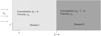
A schematic of a rectangular Hele-Shaw cell is shown in figure 1. A Newtonian incompressible fluid of species  $A$ with viscosity
 $\eta _A$ displaces another fluid of species
 $B$ with a uniform velocity
 $U_0$ along the
 $x$ direction. We consider that the composition of the system is uniquely determined through the molar fraction
 $\phi$ of species
 $A$. Since we are considering a binary mixture, we thus assume the molar fraction of species
 $B$ to be
 $1-\phi$. The governing equations consist of continuity, momentum and mass transport equations in a reference frame moving with the injection velocity
 $U_0$ and can be expressed as (Vladimirova, Malagoli & Mauri Reference Vladimirova, Malagoli and Mauri1999a,Reference Vladimirova, Malagoli and Maurib; Hopp-Hirschler, Shadloo & Nieken Reference Hopp-Hirschler, Shadloo and Nieken2019)
 \begin{gather} \boldsymbol{\nabla}\boldsymbol{\cdot} \boldsymbol{U} = 0, \end{gather}
 \begin{gather}\frac{\eta}{\mathcal{K}} (\boldsymbol{U} + \boldsymbol{i}U_0 ) ={-}\boldsymbol{\nabla} P + \boldsymbol{F}, \end{gather}
 \begin{gather}\frac{\partial \phi}{\partial t} + \boldsymbol{U} \boldsymbol{\cdot}\boldsymbol{\nabla} \phi ={-}\frac{1}{\rho}\boldsymbol{\nabla}\boldsymbol{\cdot} \boldsymbol{J_A}, \end{gather}
where  $\eta$,
 $\mathcal {K}$ and
 $\boldsymbol {J_A}$ are the viscosity of the fluid mixture, the permeability of the Hele-Shaw cell and the diffusion flux of species
 $A$, respectively. We have used the concentration-dependent viscosity model,
 \begin{equation} \eta = \eta_0 \exp({-}R\phi), \end{equation}
where  $R$ is the log viscosity parameter and
 $\eta _0$ is the solute free viscosity. By assuming the molecular weight of species
 $A$ and
 $B$ to be the same, i.e.
 $M_{w,A} = M_{w,B} = M_{w}$, the Korteweg force has been expressed as (Vladimirova et al. Reference Vladimirova, Malagoli and Mauri1999a,Reference Vladimirova, Malagoli and Maurib)
 \begin{equation} \boldsymbol{F} = \left(\frac{\rho \mathcal{R} T}{M_w} \right) \bar{\mu} \boldsymbol{\nabla} \phi, \end{equation}
where,  $\bar {\mu } = \bar {\mu }_A - \bar {\mu }_B$ is the dimensionless chemical potential of the binary mixture and has been constructed as (Cahn & Hilliard Reference Cahn and Hilliard1958; Vladimirova et al. Reference Vladimirova, Malagoli and Mauri1999a,Reference Vladimirova, Malagoli and Maurib)
 \begin{gather} \bar{\mu} = \frac{\mu}{\mathcal{R}T} = \frac{\mu_A - \mu_B}{\mathcal{R}T} = \bar{\mu}_A - \bar{\mu}_B = \bar{\mu}_{Th} + \bar{\mu}_{NL}, \end{gather}
 \begin{gather}\bar{\mu}_{Th}\left( = \frac{\partial \bar{g}_{Th}}{\partial \phi} \right) = \ln \left(\frac{\phi}{1-\phi} \right) + \varPsi(1-2\phi) \quad \text{and} \quad \bar{\mu}_{NL}\left(= \frac{\partial \bar{g}_{NL}}{\partial \phi} \right) ={-} \kappa \nabla^2 \phi, \end{gather}
 \begin{gather}\bar{g}_{Th}\left( = \frac{g_{Th}}{\mathcal{R}T} \right) = \{ \phi \ln \phi + (1-\phi)\ln(1-\phi) \} + \varPsi \phi(1-\phi), \end{gather}
 \begin{gather}\bar{g}_{NL}\left( = \frac{g_{NL}}{\mathcal{R}T} \right) ={-} \frac{1}{2} \kappa^2 (\boldsymbol{\nabla} \phi_A)(\boldsymbol{\nabla} \phi_B), \end{gather}
where,  $\bar {\mu }_{Th}$ and
 $\bar {g}_{Th}$ are the dimensionless chemical potential and thermodynamic free energy for the equilibrium state, respectively. Here
 $\bar {\mu }_{NL}$ and
 $\bar {g}_{NL}$ are added to take into account the effects of spatial inhomogeneities. For a binary mixture, we define
 $\phi _A = \phi$ and
 $\phi _B = (1-\phi )$ as the molar fraction of species
 $A$ and
 $B$, respectively. The Margules parameter is
 $\varPsi$, which describes the repulsive interaction between unlike molecules versus that between like molecules, and
 $\kappa$ is the gradient parameter that is proportional to the effective interfacial tension (Cahn & Hilliard Reference Cahn and Hilliard1958). Here,
 ${\kappa }$ has the meaning of the square of the thermodynamic length scale (Cahn & Hilliard Reference Cahn and Hilliard1958; Vladimirova et al. Reference Vladimirova, Malagoli and Mauri1999a,Reference Vladimirova, Malagoli and Maurib). For various systems, many systematic studies (Ariyapadi & Nauman Reference Ariyapadi and Nauman1990; Nauman & He Reference Nauman and He1994; Zhou & Powell Reference Zhou and Powell2006; Morita Reference Morita2013) have been conducted to determine the Margules parameter,
 $\varPsi$, and the gradient energy parameter,
 $\kappa$.
Schematic diagram of the system considered where a less viscous fluid with viscosity  $\eta _A$ is displacing a more viscous fluid with viscosity
 $\eta _B$.

In the regular solution theory, the first term of  $\bar {g}_{Th}$, i.e.
 $\{ \phi \ln \phi + (1-\phi )\ln (1-\phi ) \}$, expresses the entropy of mixing, and the second term,
 $\varPsi \phi (1-\phi )$, explains the enthalpy of mixing. This expression is of the same form as the Flory–Huggins equation of state that is commonly used for polymer mixtures (Flory Reference Flory1942; Huggins Reference Huggins1942). If
 $\varPsi > 2$, there exists a thermodynamically unstable partially miscible region (called the spinodal region) where
 \begin{equation} \frac{\partial \bar{\mu}_{Th}}{\partial \phi}\left(= \frac{\partial^2 \bar{g}_{Th}}{\partial \phi^2} \right) < 0 \end{equation}
(Lee, Lowengrub & Goodman Reference Lee, Lowengrub and Goodman2002; Lamorgese & Mauri Reference Lamorgese and Mauri2006; Suzuki et al. Reference Suzuki, Tada, Hirano, Ban, Mishra, Takeda and Nagatsu2021). Margules parameters have been shown to be dependent on temperature and, hence, the miscibility can be controlled by changing temperature (Vorobev, Prokopev & Lyubimova Reference Vorobev, Prokopev and Lyubimova2021). In this work, however, we have not studied the temperature effects on the VF. To represent the stable and unstable mixture, Hopp-Hirschler et al. (Reference Hopp-Hirschler, Shadloo and Nieken2019) adopted  $\varPsi = 1$ and
 $\varPsi =3$, respectively.
Originally, Cahn & Hilliard (Reference Cahn and Hilliard1958) expressed the mass flux as
 \begin{equation} \boldsymbol{J_A} ={-}\rho M \boldsymbol{\nabla} \bar{\mu}_{A}, \end{equation}
where  $M$ corresponds to the mobility coefficient that corresponds to the diffusion coefficient (Jasnow & Vinals Reference Jasnow and Vinals1996). However, as discussed by Nauman & Balsara (Reference Nauman and Balsara1989), the above expression is inconsistent with the modern diffusion theory (Bird, Stewart & Lightfoot Reference Bird, Stewart and Lightfoot2002; Cussler Reference Cussler2009). The mass flux for each component of species
 $(i=A \ \text {or} \ B)$ in the system is expressed by using the gradient of chemical potential as
 \begin{gather} \boldsymbol{J}_i ={-} \rho \phi_i(\boldsymbol{U}_i - \boldsymbol{U}), \end{gather}
 \begin{gather}\boldsymbol{U}_i ={-}M\boldsymbol{\nabla} \bar{\mu}_i, \end{gather}
and the mass average velocity  $\boldsymbol {U}$ is expressed as
 \begin{equation} \boldsymbol{U} = \sum_i\phi_i \boldsymbol{U}_i. \end{equation}
By combining (2.9) and (2.10), the mass flux of species A can be reduced to
 \begin{equation} \boldsymbol{J_A} ={-} \rho \phi(1-\phi)M \boldsymbol{\nabla} \bar{\mu}. \end{equation}
Substituting the expressions for mass flux (2.11) and force (2.5), we arrive at our modified HSCH model. The governing equations are non-dimensionalized using
 \begin{equation} \bar{\eta} = \frac{\eta}{\eta_0}, \quad \boldsymbol{u}= \frac{\boldsymbol{U}}{U_0}, \quad \bar{x} = \frac{x}{M/U_0} \quad \tau = \frac{t}{M/U_0^2}, \quad p = \frac{P}{(\eta_0 M)/\mathcal{K}}. \end{equation}
The governing equations thus reduce to
 \begin{gather} \boldsymbol{\nabla} \boldsymbol{\cdot} \boldsymbol{u} = 0, \end{gather}
 \begin{gather}\bar{\eta}(\boldsymbol{u} + \boldsymbol{i} ) ={-}\boldsymbol{\nabla} p + \frac{1}{Ca} \bar{\mu} \boldsymbol{\nabla} \phi, \end{gather}
 \begin{gather}\frac{\partial \phi}{\partial \tau} + \boldsymbol{u} \boldsymbol{\cdot}\boldsymbol{\nabla} \phi = \boldsymbol{\nabla} \boldsymbol{\cdot} \{\phi(1-\phi) \boldsymbol{\nabla} \bar{\mu} \} , \end{gather}
where, capillary number  $(Ca)$ is defined as
 \begin{equation} Ca = \frac{M_w \eta_0 M}{\rho \mathcal{R}T \mathcal{K}} \end{equation}
and  $\bar {\kappa } = {\kappa }/{\mathcal {K}}$. Using the expression of
 $\bar {\mu }$ from (2.6b), the Korteweg force (2.5) can be rewritten as the sum of the gradient of the scalar and the divergence of the tensor, i.e.
 \begin{equation} \boldsymbol{F} = \frac{\rho \mathcal{R} T}{M_w} \boldsymbol{\nabla} \left\{ \ln \frac{\phi}{1-\phi} + \varPsi(1 - 2\phi) + 2\kappa(\boldsymbol{\nabla}\phi \boldsymbol{\cdot}\boldsymbol{\nabla} \phi) \right\} - 2\kappa\frac{\rho \mathcal{R}T}{M_w} \boldsymbol{\nabla}\boldsymbol{\cdot} (\boldsymbol{\nabla} \phi \boldsymbol{\nabla} \phi). \end{equation}
Therefore, (2.14) can be rewritten as
 \begin{equation} \bar{\eta}(\boldsymbol{u} + \boldsymbol{i} ) ={-}\boldsymbol{\nabla} {\rm \pi}+ \delta \boldsymbol{\nabla}\boldsymbol{\cdot} (\boldsymbol{\nabla} \phi\boldsymbol{\nabla} \phi), \end{equation}
where
 \begin{equation} {\rm \pi}= p - \frac{1}{Ca}\{\phi \ln \phi + (1-\phi)\ln(1-\phi) + \varPsi (\phi-\phi^2) \} - \frac{\delta}{2}(\boldsymbol{\nabla}\phi \boldsymbol{\cdot}\boldsymbol{\nabla} \phi). \end{equation}
Here,  $\delta = \bar {\kappa } / Ca = \rho \mathcal {R}T \kappa / (M_w \eta _B M)$ has been known as the dimensionless Korteweg stress constant (Pramanik & Mishra Reference Pramanik and Mishra2013, Reference Pramanik and Mishra2015).
Under the assumption of  $0 < \psi <1$, i.e. without the consideration of a partially miscible effect, Pramanik & Mishra (Reference Pramanik and Mishra2013, Reference Pramanik and Mishra2015) degenerated the above equations (2.15) and (2.18) as
 \begin{gather} \bar{\eta}(\boldsymbol{u} + \boldsymbol{i}) ={-}\boldsymbol{\nabla}\{p + Q(\phi) \} + \delta \boldsymbol{\nabla} \boldsymbol{\cdot} (\boldsymbol{\nabla} \phi \boldsymbol{\nabla} \phi), \end{gather}
 \begin{gather}\frac{\partial \phi}{\partial \tau} + \boldsymbol{u} \boldsymbol{\cdot}\boldsymbol{\nabla} \phi = \boldsymbol{\nabla} \boldsymbol{\cdot} (\boldsymbol{\nabla} \phi), \end{gather}
where  $Q(\phi ) = {\delta }/{3} (\boldsymbol {\nabla }\phi \boldsymbol {\cdot }\boldsymbol {\nabla } \phi ) + \frac {2}{3} \gamma \nabla ^2 \phi$. For the limiting case of
 $\delta \rightarrow 0$, the above equations can be written as
 \begin{gather} \bar{\eta}(\boldsymbol{u} + \boldsymbol{i}) ={-}\boldsymbol{\nabla} {\rm \pi}, \end{gather}
 \begin{gather}\frac{\partial \phi}{\partial \tau} + \boldsymbol{u} \boldsymbol{\cdot}\boldsymbol{\nabla} \phi = \boldsymbol{\nabla}\boldsymbol{\cdot} \{\bar{D}(\phi) \boldsymbol{\nabla} \phi \}, \end{gather}
where  $\bar {D}(\phi ) = 1 - 2\varPsi \phi (1-\phi )$ is the concentration-dependent dimensionless diffusivity (Lamorgese & Mauri Reference Lamorgese and Mauri2006). Furthermore, in the dilute solution limit, i.e.
 $0<\phi <1$, and/or for the regular solution,
 $0 < \varPsi < 1$, we can reconstruct the VF model similar to Tan & Homsy (Reference Tan and Homsy1986).
2.1. Streamfunction-vorticity formulation and numerical solution method
In the present study we choose the interface at  $x=0$, where the length and the width of the domain are
 $L_x=[-1000,1000]$ and
 $L_y=[-250,250]$, respectively. For the two-dimensional (x,y) domain, we introduce the streamfunction
 $\psi$, such that
 $u = \partial \psi /\partial y$ and
 $v= - \partial \psi /\partial x$. Then, following the procedure suggested by Tan & Homsy (Reference Tan and Homsy1986), we get the following streamfunction
 $(\psi )$- vorticity
 $(\omega _z)$ formulation:
 \begin{gather} \nabla^2 \psi ={-}\omega_z, \end{gather}
 \begin{gather}\omega_z ={-}R \left\{ \frac{\partial \psi}{\partial x} \frac{\partial \phi}{\partial x} + \frac{\partial \psi}{\partial y}\frac{\partial \phi}{\partial y} + \frac{\partial \phi}{\partial y} \right\} + \frac{1}{\eta Ca} \left\{ \frac{\partial \bar{\mu}}{\partial x} \frac{\partial \phi}{\partial y} - \frac{\partial \bar{\mu}}{\partial y} \frac{\partial \phi}{\partial x} \right\} , \end{gather}
 \begin{gather}\frac{\partial \phi}{\partial \tau} + \frac{\partial \psi}{\partial y} \frac{\partial \phi}{\partial x} - \frac{\partial \psi}{\partial x} \frac{\partial \phi}{\partial y} = \boldsymbol{\nabla} \boldsymbol{\cdot} \{\phi(1-\phi)\boldsymbol{\nabla} \bar{\mu}\} . \end{gather}
As shown in the above equations, the present system is governed by  $R$,
 $Ca$,
 $\varPsi$ and
 $\bar {\kappa }$. In this work, however, we will be focusing on the effect of the later three on the phase separation and, hence, on the VF.
We consider the following initial and boundary conditions:
 \begin{gather} \psi = 0 \quad \text{and} \quad \phi(\tau=0) = \begin{cases} \phi_+, & \text{$x > 0$}, \\ \phi_{-}, & \text{$x < 0$}, \end{cases} \end{gather}
 \begin{gather}\frac{\partial \psi}{\partial x}= \frac{\partial \phi}{\partial x} = 0 \quad \text{at} \ x ={\pm} \frac{l_x}{2}, \end{gather}
 \begin{gather}\frac{\partial \psi}{\partial y}= \frac{\partial \phi}{\partial y} = 0 \quad \text{at} \ y ={\pm} \frac{l_y}{2}. \end{gather}
To perturb the concentration field, initially we added random disturbance with the magnitude of  $10^{-3}$ at
 $x=0$.
2.2. Modelling in COMSOL multiphysics software
To realize the thermodynamic approaches on a numerical solution, we implemented an in-house numerical simulation platform using a finite element method (FEM) solver (COMSOL software) (COMSOL 2019). The COMSOL software was adjusted to incorporate a thermodynamic approach and boundary conditions, interface, etc. The commercial package, COMSOL multiphysics has many built-in modules for the well-known types of governing equations with boundary conditions, and specific application fields. However, the present governing equations (2.24)–(2.26) are quite different from the typical physics model because hydrodynamics is tangled with thermodynamics. Due to the hydrodynamic-thermodynamic complexity, the present problem cannot be solved by the COMSOL built-in modules such as Darcy's law flow  $(dl)$ and the transport of dilute species
 $(tds)$ modules. Instead, we implemented an in-house numerical simulation platform using a COMSOL FEM server incorporated with thermodynamic analysis, material function and boundary conditions.
There are several equations that are included in the built-in mathematics interfaces of the COMSOL multiphysics software, for example, wave form partial differential equation (PDE), coefficient form PDE, general form PDE, etc. Each of these equations are specified with corresponding abbreviated forms in the mathematics interface. Poisson's equation (abbreviated as ‘poeq’ in the mathematics interface of COMSOL software) is used to solve (2.24) and (2.25). The equation solved by the Poisson equation in COMSOL is
 \begin{equation} \boldsymbol{\nabla}\boldsymbol{\cdot} ({-}c \boldsymbol{\nabla} \psi) = f, \end{equation}
where,  $\boldsymbol {\nabla } = [{\partial }/{\partial x}, {\partial }/{\partial y}]$. Comparing with our model equation, (2.24),
 $c$ is substituted as
 $-1$ and the source term
 $f$ is represented as
 $-\omega _z$ as given in (2.25). Equations (2.6b) and (2.26) on the other hand are solved by a general form PDE equation (abbreviated as ‘
 $g$’ in the mathematics interface of COMSOL software), which is expressed as
 \begin{equation} e_a\frac{\partial^2 \boldsymbol{u}}{\partial t^2} + d_a \frac{\partial \boldsymbol{u}}{\partial t} + \boldsymbol{\nabla}\boldsymbol{\cdot} \varGamma = f , \end{equation}
where  $\boldsymbol {u} = [\phi, \bar \mu ]^{\rm T}$ and
 $\boldsymbol {\nabla } = [{\partial }/{\partial x}, {\partial }/{\partial y}]$,
 $\varGamma$ is the conservative flux and
 $f$ is the source term. Therefore, the general form PDE is used to solve both for
 $\phi$ and
 $\bar {\mu }$. The equivalence of (2.29) and (2.26) can be understood as follows. Using the continuity equation, (2.26) can be reduced to
 $$\begin{gather} \frac{\partial \phi}{\partial \tau} + \boldsymbol{\nabla}\boldsymbol{\cdot} [( \phi^2 - \phi)\boldsymbol{\nabla} \bar{\mu} + \phi \boldsymbol{u}] = 0. \end{gather}$$
The above equation is comparable to (2.29), when we substitute the mass coefficient,  $e_a = 0$, damping coefficient,
 $d_a = 1$, and source term,
 $f = 0$, so that the flux will be
 \begin{gather} \varGamma_x = ( \phi^2 - \phi)\frac{\partial \bar{\mu}}{\partial x} + \phi \frac{\partial \psi}{\partial y}, \end{gather}
 \begin{gather}\varGamma_y = ( \phi^2 - \phi)\frac{\partial \bar{\mu}}{\partial y} - \phi \frac{\partial \psi}{\partial x}. \end{gather}
By rearranging, (2.6b) can be expressed as
 \begin{equation} \boldsymbol{\nabla} \boldsymbol{\cdot} (-\kappa \boldsymbol{\nabla} \phi) = \bar{\mu} - \ln \phi + \ln (1-\phi) - \varPsi(1-2\phi) \end{equation}
and, hence, will be comparable to (2.29), when we consider  $e_a = 0$,
 $d_a = 0$,
 $f = \bar {\mu } - \ln (\phi ) + \ln (1-\phi ) - \varPsi (1-2\phi )$ and the flux as
 $\varGamma _x = -\kappa ({\partial \phi }/{\partial x}), \varGamma _y = -\kappa ({\partial \phi }/{\partial y})$. We use initial boundary conditions,
 $\bar {\mu } = 0$ and
 ${\partial \phi }/{\partial t} = 0$, and
 ${\partial \bar {\mu }}/{\partial t} = 0$.
For the numerical simulation, we consider a user-controlled quadrilateral mesh where the maximum element size used is  ${{\rm d}\kern 0.06em x}=2$ and the minimum element size is fixed as
 $0.01$. For the time integration, we used the second-order backward difference formula (BDF) with a relative tolerance of
 $10^{-4}$. We have used an adaptive time stepping. A detailed description of the simulation parameters particularly chosen based on the intensive mesh convergence test is discussed in Appendix A.
3. Results and discussion
In the present work we have demonstrated the role of thermodynamic instabilities in phase separation of two partially miscible fluids. Unlike the work of Seya et al. (Reference Seya, Suzuki, Nagatsu, Ban and Mishra2022), in our effort to model a continuum case in this paper, we approach the problem from a solution thermodynamics perspective, within the framework of a regular solution model. Hence, we construct the Gibbs free energy such that it comprises of an entropy term and an enthalpy term as shown in the expression of  $\bar {g}={g}/{\mathcal {R} T}$ in (2.6c). The entropy term considered in this work is purely configurational in nature and emanates out of standard statistical thermodynamics. Using Stirling's approximation, this is evaluated as
 $\bar {s}= {s}/{\mathcal {R} T} = \phi \ln \phi +(1-\phi ) \ln (1-\phi )$ and provides us with a measure of disorder in the system. When considered together with the approach of Cahn and Hilliard, the concentration,
 $\phi$, is in fact the order parameter. In this work the enthalpy effects, resulting from intermolecular interactions, are captured using Margules parameter. The Margules parameter captures the net intermolecular interactions (i.e. a combination of attractive and repulsive) in the fluid system. A negative value of the Margules parameter results in attractive interactions whereas a positive value of the Margules parameter denotes a repulsive interaction. Thus, the key philosophical difference of this work with Seya et al. (Reference Seya, Suzuki, Nagatsu, Ban and Mishra2022) is that (i) we incorporate the role of disorder induced by mixing of two partially miscible fluids, and (ii) we capture the net effect of repulsion and attraction using a single term captured by the Margules parameter. Essentially, the difference between the two approaches is one that exists between a classical Landau model and a regular solution model. A consequence of this is that the double well structure of Gibbs free energy arises as a play-off between enthalpy and entropy as opposed to attractive and repulsive interactions. It is in this backdrop that we discuss our results in the following sections of this paper.
3.1. Effect of Margules parameter,  $\varPsi$, and the role of the Korteweg force

For the case of  $R=1$,
 $\kappa =1$,
 $Ca=1$,
 $\varPsi =2.2$,
 $\phi _A=0.8$ and
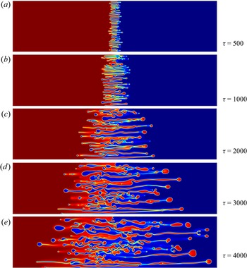
 $\phi _B=0.2$, the temporal evolution of the concentration field is summarized in figure 2. This figure clearly shows the formation of the island structure in the concentration field, which cannot be expected in the conventional fully miscible and immiscible VF problem. We can observe the formation of droplets at
 $\tau =1000$ and, as time progresses, the size of the droplets increase and become prominent.
Temporal evolution of the concentration field is shown at dimensionless time for the case of  $R=1$,
 $\kappa =1$,
 $Ca=1$,
 $\varPsi =2.2$,
 $\phi _A=0.8$ and
 $\phi _B=0.2$.

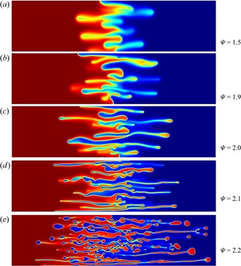
The spatio-temporal evolution of the system for different values of  $\varPsi$ is shown in figure 3. At lower values of
 $\varPsi$, a thermodynamic instability leading to phase separation is not observed
 $(\varPsi =1.5,1.9)$. In the absence of the instability, viscous fingers develop and grow into the two fluids, but further phase separation at the fingertips is not observed. The Margules parameter of
 $\varPsi =2.0$ denotes a critical point where the tip of the fingers growing into one fluid gets enriched in concentration similar to the second fluid. Once this enrichment becomes stable, this region will not remain in equilibrium with a continuously varying lower concentration and will want to phase separate. As
 $\varPsi$ is increased to
 $2.1$ though, we move beyond the critical point and the first droplet is observed. With a further increase in the value of
 $\varPsi$, the thermodynamic potentials simply drive the instabilities more strongly resulting in a more pronounced effect of phase separation and a large number of droplets form. The effect of
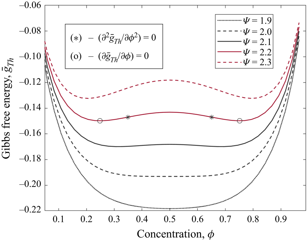
 $\varPsi$ on the thermodynamic instability can be understood from (2.6c) detailing the variation of the Gibbs free energy with
 $\varPsi$ and is shown in figure 4. Effectively, from the expression it can be seen that the contribution due to
 $\varPsi$ is equivalent to the contribution due to enthalpy, while the logarithmic terms denote the entropic contributions. Furthermore, (2.6c) assumes a regular solution model – hence, the variation of free energy is symmetric. With the value of
 $\phi$ varying between
 $0$ and
 $1$, the entropic contribution remains fixed for a given value of
 $\phi$ and assumes a minimum value
 $(\bar {s} = {s}/{\mathcal {R}T} =\phi \ln \phi +(1-\phi )\ln (1-\phi ))$ of
 $-0.693$ at the equimolar concentration. In other words, the entropy of the systems serves to lower the free energy of a system containing a mixture of two fluids and, hence, stabilizes it. Negative values of
 $\varPsi$ will also play a similar role corresponding to negative formation enthalpies that also stabilize the system. Physically, a highly negative value of
 $\bar {g}={g}/{\mathcal {R}T}$ indicates that the two-fluid system, when mixed together, is stable; in other words, it would indicate that the two fluids would not tend to phase separate. On the other hand, should the enthalpy bring about a positive contribution, which can occur for positive values of
 $\varPsi$, the system can have a maxima, as shown in figure 4. Additionally, due to the symmetric variation of enthalpy with concentration, the maxima would also occur at the equimolar concentration. Therefore, the value of the Margules parameter determines the possibility of thermodynamic instabilities within the system, with strongly positive values favouring thermodynamic instabilities that lead to spinodal decomposition. The regions of thermodynamic stability, instability and metastability can be understood by considering the variation of
 $(\partial \bar {g}/ \partial \phi )$ and these points have also been indicated in the figure for the case of
 $\varPsi =2.2$. The mixture of composition in the range of
 $0.3679 < \phi < 0.6321$ is thermodynamically unstable, which is the spinodal region, the regions
 $0.2485 < \phi < 0.3679$ and
 $0.6321< \phi < 0.7515$ are the metastable states. Here the spinodal points are obtained by solving
 ${\partial ^2 \bar {g}_{Th}}/{\partial \phi ^2} = 0$ and the binodal points are obtained for
 ${\partial \bar {g}_{Th}}/{\partial \phi } = 0$. In the metastable region the system is stable unless there is large fluctuations. In addition to the bulk thermodynamics terms (i.e. the entropic contributions,
 $\bar {s} = {s}/{\mathcal {R} T} = \phi \ln \phi +(1-\phi )\ln (1-\phi )$ and the enthalpy contributions arising due to the Margules parameter,
 $\bar {h} = {h}/{\mathcal {R}T} =\varPsi \phi (1-\phi )$), whenever two fluids mix partially, an interface will form. The interfacial region is a region where the molecular configurations change leading to local disruptions in bonding, and this is the origin of the interfacial energy that also serves to destabilize the system by contribution to
 $\bar {\mu }$, as seen in (2.6b). We have included the role of the interface through the incorporation of a gradient energy parameter,
 $\bar {\kappa }$. The gradient energy parameter, as noted earlier, represents a thermodynamic length scale
 $(\sqrt {\kappa })$ and influences the interfacial thickness and concentration gradients as a function of the distance from the interface. In this section we choose to study the role of the Margules parameter,
 $\varPsi$, keeping the values of other parameters constant (i.e. we assume
 $R=1$,
 $\kappa =1$,
 $Ca=1$). The bulk concentrations of the two fluids will then be determined by figure 4 and will correspond to the two local free energy minima. The concentration across the interface however will be given by
 $\phi _A=0.8$ and
 $\phi _B=0.2$.
The density field of concentration at dimensionless time  $\tau =4000$ for the case of
 $R=1, \kappa =1, Ca=1, \phi _A=0.8$ and
 $\phi _B=0.2$.

Effect of  $\varPsi$ on the free energy. Thermodynamic free energy, for the case of
 $\varPsi =2.2$, the mixture of composition
 $0.3679<\phi <0.6321$ is thermodynamically unstable, both
 $0.2485(=\phi _{(A,eq)} )<\phi <0.3679$ and
 $0.6131<\phi <0.7515(=\phi _{(B,eq)} )$ are metastable. Within these metastable regimes, the system is stable with respect to small fluctuations but unstable with respect to large fluctuations.

The Korteweg force is thermodynamic in nature and is dependent on the free energy variations in the system, as shown in (2.5), (2.6b) and (2.6c). The Korteweg force is therefore expressed in terms of the chemical potential and is actually a function of both  $\phi$ and
 $\varPsi$. The value of
 $\phi$ at thermodynamic equilibrium is obtained from the Gibbs tangent drawn between the two ‘wells’ in the free energy curve (i.e. near the two local minima). The shape of the free energy curve (and, hence, the values of
 $\phi$) is dictated by the strength of the intermolecular interaction, i.e. the Margules parameter
 $\varPsi$. Therefore, the value of the Korteweg force at which the droplets form is directly related to the critical value of the Margules parameter,
 $\varPsi$, for a given value of the log viscosity parameter.
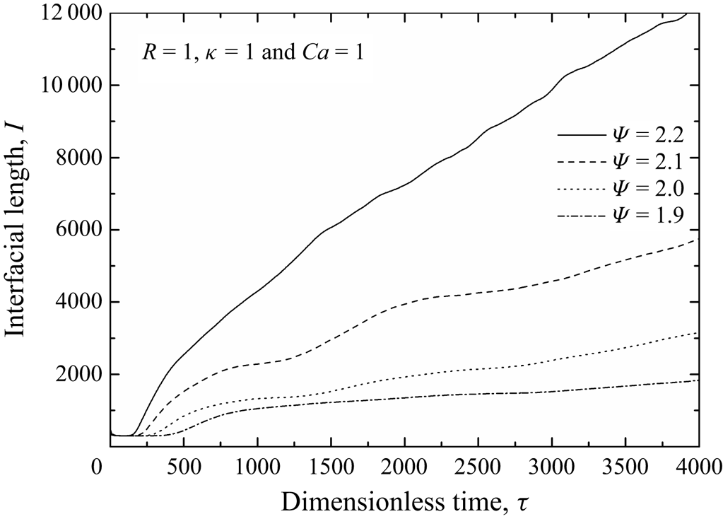
Physically, the greater the concentration fluctuations (i.e. when the concentration fluctuations are stabilized and, hence, grow), the longer the interfacial length is. Therefore, physically, as the droplets form, within the given volume of the simulation cell, the interface separating the two fluids increases. Since the formation of droplets is favoured by a larger value of the Margules parameter, this is directly reflected in the calculation of the interfacial length as shown in figure 5. Specifically, the larger values of the Margules parameter that favour the phase separation and droplet formation also result in the concentration fluctuations becoming stable and growing with time (in other words, the phase separation only increases with time). This is reflected in the slope of the curves showing the variation of the interfacial length with time in the figure. At values of  $\varPsi \leq 2$, the slope is rather low indicating that relatively less interfaces form as a function of time. At these values of the Margules parameter, the increase in interfacial length is driven by ‘stretching’ of the existing interfaces, i.e. due to a gradual increase in the extent of fingering in either fluid. A significant increase in slope is observed once we go beyond the critical value of the Margules parameter, where not only does fingering occur, but phase separation occurs concurrently resulting in splitting of the fingertips leading to droplet formation. As this process occurs and the droplets form, the interfaces (and, hence, interfacial length) increase sharply which is clearly reflected in the figure.
Effect of Margules parameter ( $\varPsi$) on the time evolution of the interfacial length for the case of
 $R=1$,
 $\kappa =1$,
 $Ca=1$,
 $\phi _A=0.8$ and
 $\phi _B=0.2$.

3.2. Effect of the capillary number, $Ca$

The thermodynamic factors primarily affect the feasibility of fingering and droplet formation. It does not, however, explicitly determine the rate. For instance, in figure 5 the variation of interfacial length with time was estimated as a function of the Margules parameter for certain values of dynamical terms such as  $Ca$ and
 $R$ (
 $Ca$ was assumed to be
 $1$, while
 $R$ was assumed to be
 $1$). The capillary number and the log viscosity affect the transport properties of the fluid, i.e. the rate at which molecular transport occurs as the system tries to evolve towards the thermodynamic equilibrium state starting from an initial non-equilibrium state. The effect of the log viscosity parameter is rather complex and will affect the viscous forces. The effect of the log viscosity parameter will be treated separately in a different paper in the future. Here, we focus on understanding the dynamics of the two-fluid systems by investigating the effect of the capillary number. The capillary number is defined in terms of the mobility parameter, which in turn affects the diffusivity. The phase separation process actually requires spatiotemporal atomic/molecular transport. Hence, the value of
 $Ca$ can be expected to influence how rapidly phase separation occurs, i.e. one can expect it to affect the temporal evolution of the interface and droplet formation.
Hopp-Hirschler et al. (Reference Hopp-Hirschler, Shadloo and Nieken2019) demonstrated that the mobility parameter plays a role in the VF process. The role of  $Ca$ has also been studied by Seya et al. (Reference Seya, Suzuki, Nagatsu, Ban and Mishra2022), where they used a dimensionless term
 $\delta ^{-1}$ that is physically equivalent to the
 $Ca$. However, despite these efforts, the role of
 $Ca$ has not been studied in isolation (i.e. independent of the intermolecular interactions). In order to do this, we have chosen a relatively large value of the Margules parameter
 $(\varPsi =2.2)$, where we know that phase separation is thermodynamically favoured. For this fixed value of Margules parameter, we now vary the capillary number over orders of magnitude and observe the interfacial region of the two-fluid system at a given time
 $(\tau =4000)$. The changes in interface morphology as a function of
 $Ca$ are shown in figure 6. The most dramatic changes occur as we move from
 $Ca = 0.01$ to
 $Ca = 0.1$. At the lowest value of
 $Ca$ studied, we observe that the concentration fluctuations have started developing at the tips of the fingers indicating an impending formation of droplets (however, at this stage, the droplets are yet to form although one can still observe the fine splitting of the fingertips that are a precursor to the droplet formation). At such low values of
 $Ca$, the mobility (and, hence, the diffusivity) of the molecular species making up the two fluids are too less for the critical amount of mass transport to have occurred in this time frame to result in phase separation. The morphological changes are somewhat quantified by calculation of the interfacial length, as discussed above. Figure 6(b) shows the evolution of the interfacial length. Beyond a certain mass transport rate (i.e. corresponding to a critical value of
 $Ca$), the changes in interfacial length are rather negligible. However, in the initial stages (low values of
 $\tau$), the interfacial length develops in a similar manner for
 $Ca = 1$,
 $10$ and
 $100$, while the interfacial length is lower for
 $Ca = 0.1$ and
 $0.01$. With time, however, the interfacial length for
 $Ca = 0.1$ becomes similar to that for
 $Ca = 1, 10$ and
 $100$. This suggests that a certain amount of mass transport needs to occur before the concentration fluctuations stabilize forming a spinodal. Spinodal decomposition is said to occur when a single phase decomposes into two similar but separate phases. This is observed in partially miscible liquids when the liquid concentrations are such that they lie beyond the miscibility limit in the immiscible region. A liquid with concentration outside the miscible range is inherently unstable thermodynamically. Statistical concentration fluctuations occur in liquid. As these fluctuations increase, the local concentration changes. Spinodal decomposition requires such fluctuations to grow since these fluctuations ensure that the local concentrations bifurcate to yield two separate concentrations that are at the boundary of the miscible range. Thus, if the concentration fluctuations are stabilized (i.e. the partitioning of the fluid phase occurs separating into two different concentration regimes), spinodal decomposition occurs. Of course, demixing does occur at the binodal point. However, for a fluid of intermediate concentration between the binodal points, to reach the binodal points, one needs to initiate the concentration changes. This occurs when the local concentration fluctuations are stable and grow sufficiently such that the single metastable fluid with a concentration between the binodal points phase separate into two fluids with concentrations that rapidly approach the binodal concentrations. The process does have a slight stochastic aspect due to the use of a random seed for introducing initial perturbations at the interface. Therefore, the number/size of droplets can be somewhat different resulting in minor differences in the interfacial length.
(a) The density field of concentration at  $\tau =4000$ to show the effect of capillary number when
 $R=1$,
 $\kappa =1$,
 $\varPsi =2.2$,
 $\phi _A=0.8$ and
 $\phi _B=0.2$. (b) Temporal evolution of the interfacial length.

3.3. Effect of the gradient parameter, $\bar {\kappa }$

The gradient parameter  $\bar {\kappa }$ is defined as
 $\bar {\kappa } = \kappa / \mathcal {K}$, i.e. the gradient energy parameter is scaled by permeability in order to obtain a dimensionless number. Thus, physically, varying the value of
 $\bar {\kappa }$ implies a change in either
 $\kappa$ or
 $\mathcal {K}$ or both. Fundamentally,
 $\kappa$ appears in Cahn–Hilliard equations as a coefficient of the concentration gradient and is related to the effective interfacial tension. In a sense, one can think of
 $\kappa$, multiplied with the concentration gradient as a measure of the energy penalty required to create an interface. Therefore, large values of
 $\kappa$ result in wider interfaces (i.e. large values of
 $\kappa$ imply a larger penalty for steeper concentration gradients – hence, wider interfaces with shallow gradients occur for large values of
 $\kappa$). Since we define
 $\bar {\kappa } = \kappa / \mathcal {K}$, large values of
 $\bar {\kappa }$ originates from large values of
 $\kappa$, for a given permeability,
 $\mathcal {K}$.
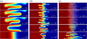
The effect of varying  $\bar {\kappa }$ can be seen in figure 7. With a progressive increase in
 $\bar {\kappa }$, the interfacial width also increases. The key question that needs to be answered though is whether
 $\bar {\kappa }$ has any significant effect on spinodal decomposition. In order to address this question, one must look jointly into the role of
 $\bar {\kappa }$ in conjunction with the Margules parameter,
 $\varPsi$. We have shown earlier that the spinodal occurs only beyond a certain critical value of
 $\varPsi$. Clearly from figure 7(a)
 $(\varPsi =0)$ and figure 7(b)
 $(\varPsi =1.5)$, one can see that droplet formation is suppressed, irrespective of the value of
 $\bar {\kappa }$. However, the interfacial width and tortuosity does change as a function of
 $\bar {\kappa }$. This is especially prominent in figure 7(a)
 $(\varPsi =0)$. As the value of
 $\bar {\kappa }$ increases, the interfacial width increases and the tortuosity of the interface reduces and we eventually approach a flat interface (figure 7(a),
 $\bar {\kappa } =10^5$). This effect is also seen on the changes in interfacial length (not shown in the figure). As the interface tortuosity decreases, the interfacial length also decreases. Physically, as the two fluids are allowed to mix, we observe a three-way thermodynamic tussle. The key factors contributing to the thermodynamic stability of such a system are (1) enthalpy – based on the intermolecular interactions, (2) entropy – based on the disorder introduced by mixing and (3) interfacial energy due to the formation of interfaces. In non-interacting systems, i.e. where
 $\varPsi =0$, the enthalpy contributions are negligible. A cursory look at the standard Gibbs free energy expression (
 $G = H -TS$, where
 $G$ is the Gibbs free energy,
 $H$ is the enthalpy,
 $T$ is the temperature and
 $S$ is the entropy) indicates that maximizing entropy by increasing disorder due to mixing will further stabilize the system by lowering the free energy. Interfaces, on the other hand, tend to increase the free energy of the system, with
 $\bar {\kappa }$, in conjunction with the concentration gradient
 $(\bar {\kappa } \boldsymbol {\nabla } \phi )$ contributing to the interfacial energy, i.e. the energy penalty associated with forming the interface. Initially, a sharp interface exists between the two fluids. As mixing of the two fluids occur, the disorder due to mixing increases. The spatial extent of the interface (i.e. the region over which the mixing occurs) is determined by a balance of entropic stabilization and the energy penalty associated with the evolution of the interface. For large values of
 $\bar {\kappa }$, a shallow concentration gradient (or low spatial concentration fluctuation) lowers the interface energy. However, a low spatial concentration fluctuation also reduces the entropy with the composition changing along a well-ordered gradient. The net result is a balancing act between the entropic stabilization (increased randomness through increased concentration fluctuation) and the energy penalty associated with the interface (lower energy associated with a shallow gradient of concentration). As the value of
 $\bar {\kappa }$ is lowered, this balance shifts towards steeper concentration gradients and higher interfacial tortuosity, which in turn results in sharper and less well-defined concentration fluctuations resulting in increased disorder and entropic contributions. All of this can be seen by observing the changes in interfacial width and tortuosity with increasing
 $\bar {\kappa }$ in figure 7(a). As the value of the Margules parameter increases (e.g. figure 7(b), where
 $\varPsi =1.5$), we observe enthalpy playing a role. Finite intermolecular interactions (though not sufficient to drive the spinodal decomposition process) contribute to stabilization of the two separate fluids. As the volume of the two fluids increase vis-à-vis volume of the interface, one observes steeper concentration gradients and a narrower interface. One can think of this as enthalpy and entropy working in tandem to stabilize the system while the interfacial energy tends to destabilize this. The addition of the enthalpy component to free energy (due to a positive Margules parameter) allows for a greater interfacial energy penalty (i.e. steeper concentration gradient, smaller interfacial width and enhanced tortuosity of the interface). All of this is reflected in figure 7(b), when compared with figure 7(a), for identical values of
 $\bar {\kappa }$.
Role of gradient parameter,  $\kappa$, on the species concentration for the case of
 $R=1$,
 $Ca=1$,
 $\phi _A=0.8$,
 $\phi _B=0.2$. Results are shown for (a)
 $\varPsi =0$ at
 $\tau =10^5$, (b)
 $\varPsi =1.5$ at
 $\tau =4000$ and (c)
 $= \varPsi =2.2$ at
 $\tau =4000$.

As the Margules parameter is further increased to  $\varPsi =2.2$ (figure 7c), one can observe that the general trend in variation of interfacial width, thickness and tortuosity remains the same; however, with the Margules parameter exceeding the critical value, spinodal decomposition resulting in the formation of droplets occur. In general, an increased value of the Margules parameter (increasing contributions of enthalpy) results in thinner, tortuous and longer interfacial lengths with steeper concentration gradients, while increasing values of
 $\bar {\kappa }$, result in shallower concentration gradients, i.e. thicker, less tortuous interfaces and smaller interfacial lengths. However, since
 $\bar {\kappa }$ and
 $\varPsi$ tend to act in opposite directions with respect to the interfacial dimensions and morphology (and, hence, droplet formation), it becomes pertinent to ask whether droplet formation can actually be suppressed by large
 $\bar {\kappa }$, even when
 $\varPsi$ is above the critical value. It turns out that this is indeed the case, as evidenced from figure 7(c), where the number of droplets reduce steadily as we increase the value of
 $\bar {\kappa }$ from
 $0.25$ to
 $100$.
3.4. Effect of asymmetricity in free energy of a binary mixture
The free energy considered in our previous subsections correspond to a symmetric binary mixture of interacting species of the same class. However, the interaction of these binary mixtures could be asymmetric as well, when the interacting particles are of a different class. Here, in this subsection we look into the effect on the free energy and concentration field when the asymmetric features of the binary system due to asymmetric inlet and outlet conditions and different sizes of solute and solvent are taken into account. Such binary mixtures are modelled by coupling the thermodynamic miscibility (Margules parameter  $\varPsi$) as a function of composition, modified Flory–Huggins equation for chemical potential (3.1) and hydrodynamic flow (capillary number
 $Ca$) (see (2.14)),
 \begin{gather} {\bar{\mu}}_{AB}\left(=\frac{\mu_A-\mu_B}{RT}\right)=\frac{\delta\bar{G}}{\delta\phi}= \ln\left(\phi\right)-\frac{1}{r_B}\ln\left(1-\phi\right)+1-\frac{1}{r_B}+\varPsi\left(1-2\phi\right)+ \kappa\nabla^2\phi. \end{gather}
Here,  $r_B$ is the relative size of molecule
 $B$ with respect to molecule
 $A$. The Flory–Huggins equation (3.1) can be easily extended to diverse mixtures of ternary, quaternary, etc. (Suzuki et al. Reference Suzuki, Nagatsu, Mishra and Ban2020a), and hence, unphysical situations are innately eliminated in the present model. Figures 8 and 9 are added to display the asymmetric effect.
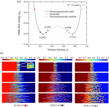
(a) Thermodynamic free energy versus concentration for  $\psi =2.2$ and
 $r_B=1$, (b) dimensionless concentration fields for the case of
 $R=1$,
 $\kappa =1$ and
 $Ca=1$ are shown at successive dimensionless times
 $\tau =1000, 2000, 3000, 4000$ from top to bottom. The numbers in the brackets are
 $[\phi _A,\phi _B]$.

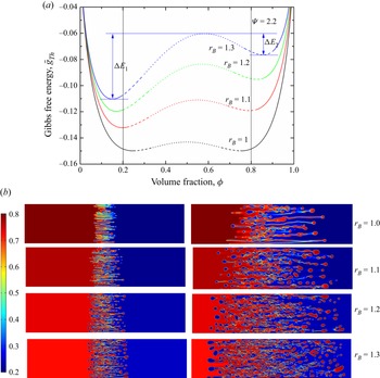
(a) Gibbs free energy for various  $r_B$ and
 $\psi =2.2$,
 $\Delta E_1$ and
 $\Delta E_2$ are the energy barriers. (b) The dimensionless concentration fields for the case of
 $R=1$,
 $\kappa =1$,
 $Ca=1$,
 $\phi _A=0.8$ and
 $\phi _B=0.2$ are shown for dimensionless times
 $\tau =1000$ (left frames),
 $\tau =3000$ (right frames). In the energy diagram, solid, dashed and dotted lines represent thermodynamically stable, metastable and unstable regions, respectively).

Figure 8(a) shows the free energy versus  $\phi$ for
 $r_B = 1$ (i.e. the ratio of energy barriers on the A rich and B rich sides are identical). The curve shown is symmetric. Here, we consider three different cases, namely: case I, (
 $\phi _A = 0.7$,
 $\phi _B = 0.1$); case II, (
 $\phi _A = 0.8$,
 $\phi _B =0.2$); case III, (
 $\phi _A = 0.9$,
 $\phi _B =0.3$). It becomes immediately apparent that case I and case III are actually quite similar, with one of the fluids having a value of
 $\phi$ that lies outside the spinodal and binodal curves completely, while the other fluid has a
 $\phi$ outside the spinodal, but inside the binodal.
For case I (left frame of figure 8b), at  $\tau = 1000$, we see three distinct concentration fields. On the right-hand side, we see a region where
 $\phi = 0.1$, with the interfacial region shifting towards higher values of
 $\phi$, as evidenced in the immediate vicinity of the fingers that form. The tips of the fully developed fingers (i.e. the fingers where we have incipient droplet formation, as marked in the inset), the concentration shifts to
 $\phi = 0.75$, which is in equilibrium with
 $\phi = 0.25$, which explains the concentration shift within the field where
 $\phi$ is largely
 $0.1$ to a value of
 $0.25$. However, the decomposition of
 $\phi = 0.7$ to
 $\phi = 0.75$ and
 $0.25$, respectively, is not an easy process, with uphill diffusion needed to overcome the energy barrier. Consequently, one observes regions where the concentration is close to the peak of the energy barrier, i.e. at
 $\phi = 0.5$. As time increases, the concentration within the binodal, i.e.
 $\phi = 0.7$, starts separating more and more into two values corresponding to
 $\phi = 0.75$ and
 $\phi = 0.25$. More and more of the fluid has already crossed the energy barrier whose peak occurs at the centre (i.e.
 $\phi = 0.5$). Therefore, concentration fields corresponding to
 $\phi = 0.5$ start dwindling progressively with increasing time and are virtually absent once we get to
 $\tau = 4000$. Essentially, the decomposition pathways involve the two-phase fluid decomposing to four distinct fields – a major field with
 $\phi = 0.1$, a thin film around fingers with
 $\phi = 0.25$, the decomposing fluid fingers with
 $\phi = 0.5$ (as the fluid tries to go past the energy barrier) and the second major concentration field of
 $\phi = 0.7$. As the
 $\phi = 0.7$ field decomposes, a part of it approaches
 $\phi = 0.5$ and then beyond, while the other part approaches
 $\phi = 0.75$ that is barely discernible from
 $\phi = 0.7$, given the contrast. With time, the decomposing fluid overcomes the energy barrier and we end up with three discernible regions of
 $\phi = 0.1$ (right far field),
 $\phi = 0.25$ (around the fingers at the interface) and
 $\phi = 0.75$ (the concentration of the fingers themselves). It is important to note that the operative word here is discernible. It is postulated that the left far field is actually
 $\phi = 0.7$, which is virtually indiscernible from the finger concentration of
 $\phi = 0.75$. Additionally, one also observes the growth of the fingers with time as we approach thermodynamic equilibrium. These observations also hold for case III (right frame of figure 8b), where
 $\phi _A$ and
 $\phi _B$ are
 $0.9$ and
 $0.3$, respectively. In case II (middle frame of figure 8b), where both points lie just outside the binodal region, the thermodynamic driving force for phase separation is not quite as high, with the gradient of free energy being quite shallow. This is quite clearly seen in the figure when compared with case I and case III. Case II does exhibit significant fingering, but very few of the fingertips reach a situation requiring complete separation or droplet formation. In case I and case III, however, droplet formation, especially at longer time intervals
 $(\tau = 4000)$, is quite prominent.
In figure 9 we revisit case II with asymmetric interactions leading to an asymmetric free energy curve where the energy barrier on one side is lower than the other. The studies are done over a range of  $r_B$ values. Two observations stand out clearly – (a) at a given time interval, a larger fraction of the fluid shows a concentration field of approximately
 $\phi = 0.5$ (or, the local maxima in the free energy curve between
 $\phi = 0.2$ and
 $0.8$); and (b) enhanced droplet formation with increasing
 $r_B$ values. Taken together, this is clearly indicative that the decomposition process becomes accelerated with increasing asymmetry where the energy barrier on one side of the concentration profile becomes significantly smaller. A lower activation barrier allows for easy diffusion and, hence, faster redistribution of the concentration field – hence, a smaller fraction of the fluid needs to reside close to the maxima (
 $\phi = 0.54$), with more and more fluid crossing over the energy barrier and moving rapidly towards the equilibrium concentration. Increasingly copious droplet formation also shows a higher degree of phase separation (which, for it to happen, it is essential that the fluid crosses the energy barrier in order to reach the equilibrium concentrations).
In all of these cases (differing values of  $\phi _A$ and
 $\phi _B$, as well as different values of
 $r_B$ for a given set of
 $\phi _A$ and
 $\phi _B$), the viscosity contrast for a particular concentration is the same, which indicates that the hydrodynamic contribution does not change. However, with different sets of
 $\phi _A$ and
 $\phi _B$, as well as different values of
 $r_B$, the hydrodynamic contribution does change the thermodynamic driving forces – which is reflected in changing temporal signatures/kinetics of the spinodal decomposition process. This quite clearly demonstrates the significance of thermodynamic driving forces during spinodal decomposition occurring at the interfacial region during partial mixing of fluids, with the effect being especially pronounced under the asymmetric interaction (Margules) parameter, concentrations within the binodal region and concentrations with a high
 $\partial G / \partial \phi$.
3.5. Liesegang rings in the thermodynamically unstable system
While the parametric studies provide insights into the VF and droplet formation process, applying this approach to explain real-life scenarios provides an excellent test of this model. One of the areas where VF plays a role is in the formation of the Liesegang rings and, hence, the ability to replicate the formation of Liesegang rings under suitable conditions can be a means of validating our model. Liesegang rings or bands are colour bands or ring-like structures and are commonly observed in chemical reaction systems (Kai Reference Kai1985). The physical mechanism of such a process is yet to be understood, however, the prevailing theory is the post-nucleation theory and is based on the Ostwald ripening process (Hilhorst et al. Reference Hilhorst, van der Hout, Mimura and Ohnishi2009), commonly found in aqueous two-phase system solutions (Zhang et al. Reference Zhang, Trabbic-Carlson, Albertorio, Chilkoti and Cremer2006) where advection is completely dominated by diffusion. Numerical simulations of such models have been explored in the literature. For instance, Hopp-Hirschler et al. (Reference Hopp-Hirschler, Shadloo and Nieken2019) conducted their numerical simulations using the viscosity model
 \begin{equation} \eta=\eta_0(1+\beta \phi) \end{equation}
rather than the conventional viscosity model (2.4). In their simulations for the miscible system, they employed  $\varPsi =3$,
 $\beta =2$,
 $\phi _A=0.5$,
 $\phi _B=0.0$. As discussed in figure 4, their system is partially miscible for
 $\varPsi > \varPsi _c(=2)$, the displacing phase is thermodynamically unstable and the displaced phase is thermodynamically stable. They explained these rhythmic patterns as Liesegang rings that are self-generated patterns observed in a supersaturated solution (Ostwald Reference Ostwald1897). Later, Falkovitz & Keller (Reference Falkovitz and Keller1988) analysed the Liesegang pattern formation in a precipitation system using the Cahn–Hilliard equation. They proposed that the negative diffusion coefficient is the key factor for the Liesegang pattern formation. Since supersaturation and uphill diffusion are related to thermodynamic instability, to examine the occurrence of the rhythmic patterns obtained previously by (Hopp-Hirschler et al. Reference Hopp-Hirschler, Shadloo and Nieken2019), we constructed a thermodynamically unstable model system by considering
 $\varPsi =2.2$,
 $\phi _A=0.9$,
 $\phi _B=0.5$ and
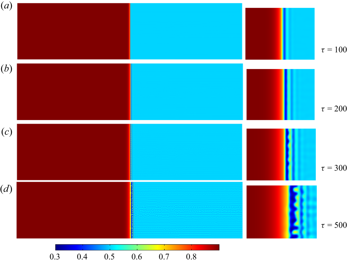
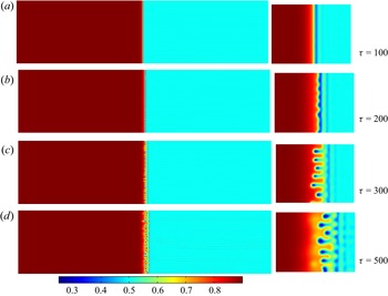
 $R=1$. For these parameters, the temporal evolution of both the hydrodynamically and thermodynamically unstable system is shown in figure 10 and we clearly observe the rhythmic concentration profile patterns near the interface. Similarly, Liesegang bands with fingering motions caused by the phase separation effects are also clearly visualized in figure 11, where the temporal evolution of the concentration field is shown. In this case, the thermodynamically unstable model is constructed by taking
 $\varPsi =2.2$,
 $\phi _A=0.9$,
 $\phi _B=0.5$, on the other hand, a hydrodynamically unstable system is constructed by considering
 $R=-1$.
Temporal evolution of the concentration field for the case of  $R=1$,
 $\kappa =1$,
 $Ca=1$,
 $\varPsi =2.2$,
 $\phi _A=0.9$ (thermodynamically stable) and
 $\phi _B=0.5$ (thermodynamically unstable). Upper centre parts are enlarged in the right panels.

Temporal evolution of the concentration field for the case of  $R=-1$,
 $\kappa =1$,
 $Ca=1$,
 $\varPsi =2.2$,
 $\phi _A=0.9$ (thermodynamically stable) and
 $\phi _B=0.5$ (thermodynamically unstable). Upper centre parts are enlarged in the right panels.

Therefore, our mathematical model could rightly replicate the interesting formation of Liesegang bands that occur due to thermodynamic instability. However, an in-depth analysis on the formation of rings and dynamics of such pattern formation requires a comprehensive study.
4. Conclusions
Phase separation in a partially miscible system has been systematically analysed numerically. Using the Hele-Shaw cell approximation and incorporating the Korteweg force, Cahn–Hilliard phase field model and Flory–Huggins mixing energy, new governing equations were derived to cover the thermodynamic and hydrodynamic instabilities. The governing equations are solved through in-house model implementation using the commercially available FEM solver COMSOL multiphysics. We have been able to distinguish the development and dynamics of VF due to the hydrodynamic and thermodynamic changes. The growth and shape of fingering and the formation of droplets are shown to be affected by thermodynamic changes, for example, the Margules parameter and gradient parameter. However, temporal evolution and dynamics at the interface are affected by kinetics, e.g. capillary number. We show that the capillary number, gradient parameter and the Margules parameter play an important role in the VF. The gradient parameter, which is linked to the capillary number, has an effect in both thermodynamic and hydrodynamic features and serves to link both these effects. The effects of these physico-chemical parameters have been studied systematically. We have also demonstrated that thermodynamic driving forces have a stronger effect under an asymmetric interaction parameter. The present study provides a robust physical basis to study phase changing effects on the VF in multicomponent systems.
Funding
M.C.K. acknowledges the support of the Basic Science Research Program through the National Research Foundation of Korea (NRF) funded by the Ministry of Education (NRF-2021R1I1A3A04037444). M.M. acknowledges financial support from SERB, Government of India, through project grant no. CRG/2020/000613. L.P. acknowledges the support from DST, Government of India through grant no. DST/WOS-A/PM-23/2020(G).
Declaration of interests
The authors report no conflict of interest.
Appendix A. Convergence and mesh independence study
In the in-house COMSOL model implementation the time/space/boundary conditions are controllable. The model implementation has been validated through several simulation cases matching with experimental works. The numerical simulation solver is also implemented with good convergence and accuracy. For the numerical solution of the flow geometry, in the present simulation we use spatial discretization with the FEM, where the calculation domain is subdivided into finite elements such as rectangle (user-controlled free-quadrilateral elements). In each rectangle the physical quantity is approximated as a combination of piecewise continuous bilinear functions. For numerical simulation, equations are discretized according to the FEM. To benchmark our simulations and examine the accuracy, we consider the case with  $\varPsi =2.2$,
 $R=1$,
 $Ca=1$,
 $\kappa =1$ and perform several simulation sets considering different meshes. To choose the appropriate mesh size, we perform our simulations choosing
 ${{\rm d}\kern 0.06em x}={{\rm d}y}$ and varying the maximum element size
 ${{\rm d}\kern 0.06em x} = \{16, 8, 4, 2, 1.55 \}$, fixing the minimum element size to
 $0.01$. The total degrees of freedom (DOF) for each of the mesh sizes is shown in table 1. The effect of mesh size is demonstrated via interfacial length
 $(I)$ (A1), which is a measure of the distortion of the concentration field and is given by (Chen & Meiburg Reference Chen and Meiburg1998; Mishra et al. Reference Mishra, Martin and De Wit2008)
 \begin{equation} I = \int_{{-}l_x/2}^{l_x/2} \int_{{-}l_y/2}^{l_y/2} \sqrt{\left(\frac{\partial \phi}{\partial x}\right)^2 + \left(\frac{\partial \phi}{\partial y}\right)^2}\,{{\rm d}y} \, {{\rm d}\kern 0.06em x} \end{equation}
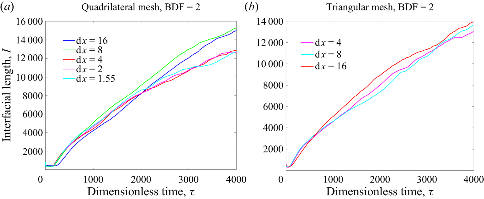
and is shown in figure 12(a). It is evident that, for  ${{\rm d}\kern 0.06em x} \leq 4$, the interfacial length converges and the behaviour remains almost similar as compared with the results with a higher grid size, i.e.
 ${{\rm d}\kern 0.06em x} \geq 4$. Hence, we chose
 ${{\rm d}\kern 0.06em x}=2$ for our investigation on the phase separation. The order of convergence of finite elements is related to the polynomial order of the basis functions used on each element. However, irregularity of the PDE solutions and the high nonlinearity in the system prevents us in achieving the order of convergence (Gobbert & Yang Reference Gobbert and Yang2008) and, hence, is not tested. Nevertheless, to validate the results, we have also performed the convergence test using free triangular (Delaunay) meshing with an automatic tessellation. The advantage of Delaunay tessellation is that the triangles are regular and are independent of the mesh. No significant changes have been observed in the profile of the interfacial lengths in comparison to quadrilateral meshing (figure 12b). It should be noted that due to computational constraint, simulations for
 ${{\rm d}\kern 0.06em x}=2$ and
 ${{\rm d}\kern 0.06em x}=1.55$ could not be done for triangular elements because of higher number of DOFs present in the system (see table 1 for comparison).
Degrees of freedom used for grid independence study.

Interfacial length to check the convergence for the quadrilateral mesh (a) and triangular mesh (b) for various spatial size.

For the mass continuity, because we used the streamfunction-vorticity formation, see (2.24)–(2.26), the mass conservation law, i.e. the continuity equation, is naturally satisfied, and solved the resulting equations by the well-known Poisson equation solver and the general form PDE solver. For interface treatment error related to smearing, smearing phenomena are unavoidable and natural for the present partially miscible binary system. It should be stressed that this study did not depend on the built-in modules of the COMSOL multiphysics, such as level set  $(ls)$ or phase field
 $(pf)$ modules. Instead, the ‘Fourier spectral method’ used in the work of Seya et al. (Reference Seya, Suzuki, Nagatsu, Ban and Mishra2022) was employed to describe smearing phenomena to solve the drop formation accompanying the VF instabilities. Nevertheless, we have also explored the mass conservation of the system for the present model. At initial time, the concentration occupies a fixed area and, hence, in order to have mass conservation, the area occupied by the concentration should remain the same for all time. To do so, we can consider that the total area occupied by the concentration at initial time and at time
 $t$ is
 \begin{equation} a_\phi(t) = a_\phi(t=0) = (\text{area of domain I} ) \phi_A + (\text{area of domain II}) \phi_B, \end{equation}
which, for our system with  $L_x=2000$ and
 $L_y = 500$, is
 $a_{\phi } \approx 500\,000$. Now, the area occupied by concentration in our numerical model can be found by computing
 \begin{equation} a_{\phi,{{\rm d}\kern 0.06em x}} = \int_\varOmega \phi \,{\rm d}\varOmega \end{equation}
by varying spatial sizes. Hence, computing the percentage error,  $E_{{\rm d}\kern 0.06em x}(t) = | a_{\phi,{{\rm d}\kern 0.06em x}} - a_\phi | / a_\phi$, we can see if mass is conserved in our system. We have presented the maximum percentage error for
 ${{\rm d}\kern 0.06em x} = 2,4,8,16$ in the case of quadrilateral meshing and
 ${{\rm d}\kern 0.06em x}=4,8,16$ for triangular meshing in table 2 using the BDF of order 2. The maximum percentage error for all time is shown to be of the order of
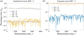
 $10^{-3}$, indicating conservation of mass in the system. Figures 13(a) and 13(b) show the percentage error with time for both quadrilateral as well as triangular meshing and mesh convergence is apparent for
 ${{\rm d}\kern 0.06em x} =2$ for quadrilateral meshing.
Maximum percentage error for mass conservation using the BDF of order 2.

Percentage error for spatial mesh sizes,  ${{\rm d}\kern 0.06em x}$.

We have used an adaptive time stepping with a relative tolerance of 0.001, which means the software automatically adjusts the time step to maintain the relative tolerance considered. Since there is no significant changes in our system immediately after the start time, we have introduced a default initial time step size. Here, to solve the system of time-dependent ordinary differential equations, we used the second-order BDF that is a family of implicit methods for the numerical integration of ordinary differential equations. Since the BDF are linear multistep methods, the integration time step is controlled by the relative errors. The effect of convergence criterion, i.e. relative error, on the onset and growth of VF instabilities and the droplet formation is summarized in figure 14. As shown in figure 14, the effect of the convergence criterion is not critical as long as the relative tolerance is  ${<}10^{-3}$. In this numerical study the relative tolerance (
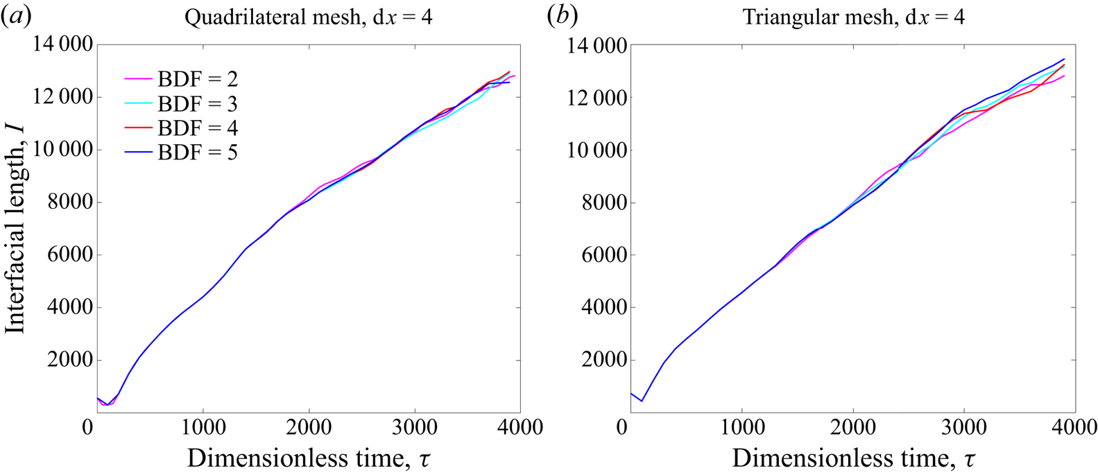
 ${=}10^{-4}$) was chosen so that numerical solutions are obtained based on the sufficiently refined time step. We have also examined even higher orders of the BDF and shown the system to be independent of the order of the BDF chosen. For example, figure 15 shows the interfacial length employing both quadrilateral and triangular meshing and it is noticeable that the profiles are similar irrespective of the order of the BDF. The maximum percentage error is also presented in table 3 for
 ${{\rm d}\kern 0.06em x}={{\rm d}y}=4$ for varying orders of the BDF and confirms mass conservation.
(a) Temporal evolution of the interfacial length for relative tolerances (Rel. tol.)  $10^{-3}$,
 $10^{-4}$,
 $10^{-5}$ for
 $\varPsi =2.2$,
 $R=1$,
 $Ca=1$,
 $\kappa =1$. (b) Concentration field for relative tolerances
 $10^{-3}$,
 $10^{-4}$,
 $10^{-5}$ (columns from left to right).

Interfacial length with  ${{\rm d}\kern 0.06em x}=4$ and increasing orders of the BDF.

Maximum percentage error for  ${{\rm d}\kern 0.06em x}={{\rm d}y}=4$ and varying BDF orders.

For our thermodynamic study of the partially miscible VF, we therefore used the spatial resolution corresponding to the mesh size  ${{\rm d}\kern 0.06em x}={{\rm d}y}=2$ and a relative tolerance of
 ${10}^{-4}$ was chosen for the present simulations.