1. Introduction
Private equity funds account for a growing share of real investment in the modern economy, accompanied by increasing scholarly interest in their nature and effects. A well-established empirical literature demonstrates that private equity significantly contributes to innovation and economic growth (Kortum and Lerner, Reference Kortum and Lerner2000; Samila and Sorenson, Reference Samila and Sorenson2011; Audretsch et al. Reference Audretsch, Lehmann, Paleari and Vismara2016). Notably, Jovanovic et al. (Reference Jovanovic, Ma and Rousseau2022) distinguish between two fundamental components: venture capital, which provides financing to startups and early-stage growth firms, and buyout funds, which acquire existing firms, optimize their operations, and subsequently exit through sales to other investors or public markets. Their estimates indicate these private equity sectors collectively contribute between 14% and 21% of US economic growth relative to a counterfactual without private equity.
Despite these significant contributions, theoretical research embedding private equity within macroeconomic frameworks remains underdeveloped, particularly regarding buyout funds. Existing studies have focused predominantly on venture capital, examining its procyclical nature (Opp, Reference Opp2019), the role of non-diversified agents’ hedging motives (Petukhov, Reference Petukhov2019), and its relationship to growth through dynamic contracts (Greenwood et al. Reference Greenwood, Han and Sánchez2022). This paper aims to fill the critical void in understanding buyout funds’ origins and their relationship with economic growth.
A fundamental challenge in modeling private equity is the “Private Equity Premium Puzzle” (Moskowitz and Vissing-Jorgensen, Reference Moskowitz and Vissing-Jorgensen2002). Empirical evidence consistently shows that private equity investments yield risk-adjusted returns no higher than public equities despite being highly concentrated and poorly diversified (Hamilton, Reference Hamilton2000; Cochrane, Reference Cochrane2005; Shane, Reference Shane2009; Hall and Woodward, Reference Hall and Woodward2010; Harris et al. Reference Harris, Jenkinson and Kaplan2014; Gupta and Van Nieuwerburgh, Reference Gupta and Van Nieuwerburgh2021). Traditional expected utility frameworks cannot explain why risk-averse investors would accept such inefficient portfolios. Crucially, survey evidence reveals that private equity suppliers are predominantly ultra-high-net-worth individuals (Rin et al. Reference Rin, Hellmann, Puri, Rin, Hellmann and Puri2013).
Inspired by these findings, we resolve this puzzle by introducing agents whose preferences shift when income exceeds a threshold: they exhibit standard concave utility for safe investments but develop convex utility for risky entrepreneurial ventures above an income threshold. This preference structure generates several empirically observed behaviors. At low income levels, agents rely exclusively on safe savings methods. As income crosses the threshold, they develop concentrated positions in risky investments without diversification, since diversification would reduce the convexity-driven utility they derive from these investments. Most importantly, they begin seeking the “thrill” of entrepreneurial activities despite suboptimal financial returns, consistent with patterns documented by Campbell (Reference Campbell2017). This approach aligns with explanations based on non-pecuniary benefits (Moskowitz and Vissing-Jorgensen, Reference Moskowitz and Vissing-Jorgensen2002; Hurst and Pugsley, Reference Hurst and Pugsley2015).Footnote 1
Our preference specification relates to recent work on heterogeneous risk attitudes in macroeconomic settings. Notably, Araujo et al. (Reference Araujo, Gama and Kehoe2025) demonstrates how risk-loving behavior at the wealth extremes can generate fat-tailed wealth distributions, while Araujo et al. (Reference Araujo, Chateauneuf, Gama and Novinski2018) presents a general equilibrium framework with uncertainty-loving preferences. Unlike these studies that focus on exogenously given preference heterogeneity, our model endogenizes risk-loving behavior through income-dependent utility curvature. Specifically, we reconcile Araujo’s observation of risk-loving wealthy investors with microfoundations: convex utility over risky assets emerges only above an income threshold, creating endogenous heterogeneity that varies with economic conditions. This mechanism complements their findings while providing new insights into how endogenous preference formation affects financial intermediation patterns.
The model features two distinct agent types differentiated by their endowments: wealthy agents who lack business ideas and poorer agents who possess them. These agents engage in Nash bargaining to establish cooperative ventures. Our modified risk preferences yield a crucial insight: the optimal contract naturally takes the form of a buyout fund.Footnote 2 Wealthy investors, motivated by the desire for entrepreneurial engagement, actively seek to acquire business opportunities, offering premiums proportional to their income. Entrepreneurs will only sell their ideas when acquisition prices adequately compensate for relinquished control. Consequently, buyout funds emerge exclusively when income inequality exceeds a certain threshold, and they disappear as incomes increase.
This dynamic mirrors real-world entrepreneurial spawning processes (Gompers et al. Reference Gompers, Lerner and Scharfstein2005). Initially, idea owners sell to funds due to capital constraints or attractive offers. However, growth-induced wage increases alter reservation utilities in bargaining. As entrepreneurs gain financial capacity and bargaining power, they retain ideas for independent implementation—the “Xerox effect” occurs precisely when inequality is moderate. Thus, buyout funds serve as transitional institutions intrinsically linked to income inequality.
The model provides valuable insights into the role of buyout funds in driving economic growth. By engaging wealthy investors in innovation processes, they increase the probability of R&D success. These successes expand the variety of intermediate goods in the economy, accelerating growth. Perhaps more significantly, the resulting wage increases enable previously constrained entrepreneurs to implement their ideas independently, creating a virtuous cycle of growth. This mechanism suggests that initial inequality can serve as a catalyst for sustained growth, with buyout funds acting as the transmission channel.
These findings make important contributions to the literature on inequality and growth. Earlier studies identified positive relationships through various channels, including physical capital investment (Galor and Moav, Reference Galor and Moav2004), and demand-driven innovation (Foellmi and Zweimüller, Reference Foellmi and Zweimüller2006). Our model establishes a novel financial intermediation channel that operates differently from these established mechanisms. The buyout funds in our framework emerge as institutions whose existence depends on inequality levels. They directly accelerate variety expansion through increased innovation success rates, while their eventual decline through endogenous wage convergence triggers widespread entrepreneurial spawning. This dual-phase process represents a distinct contribution to understanding how buyouts can temporarily stimulate R&D-driven growth while simultaneously creating conditions for their own reduction.
The remainder of this paper proceeds as follows. Section 2 presents the core model framework and details agent preferences. It derives the optimization problems for both well-endowed and under-endowed agents and characterizes the Nash bargaining solution that governs their interactions. Section 3 analyzes the resulting temporary equilibrium. Section 4 investigates the model’s long-run dynamics, establishing conditions for the persistence or disappearance of the buyout fund. Section 5 discusses growth and policy implications. Section 6 provides numerical transition paths and sensitivity analysis. Section 7 concludes.
2. The model
2.1 Agents and preferences
We propose an overlapping generations economy populated by a continuum of agents who live for two periods. Each cohort has measure
 $L\gt 0$
and is born at the beginning of period
 $t$
. Agents are of two types: a fraction
 $\theta \in (0,1/2)$
are well-endowed and the remaining
 $1-\theta$
are under-endowed. Preferences are discounted with factor
 $\beta \in (0,1)$
, entrepreneurial success is governed by a technological parameter
 $p\in (0,1)$
, and the curvature of the non-pecuniary payoff from entrepreneurial success is
 $\alpha \gt 1$
.
In the first period of life, an under-endowed agent receives
 $e^u\gt 0$
units of labor and is endowed with a business idea, while a well-endowed agent receives
 $e^w\ge e^u$
units of labor but no business concept. These labor endowments satisfy
 \begin{equation} \theta e^w + (1 - \theta )e^u = \bar {e}, \end{equation}
where
 $\bar e$
denotes average labor supply per cohort. We impose
 \begin{equation*} 0 \lt e^u \leq \bar {e} \leq e^w \lt \bar {e}/\theta , \end{equation*}
and assume labor is supplied inelastically. The restriction
 $\theta \lt 1/2$
reflects the empirical reality that ultra-high-net-worth individuals are fewer than idea-rich but capital-constrained entrepreneurs and simplifies the bargaining analysis.Footnote 3
Young agents can transfer resources to old age through two channels. First, they can carry final goods to the next period as risk-free capital loans to incumbent firms. Second, they can invest in entrepreneurial startups that create new varieties: a project yields monopoly profits if successful and zero otherwise. Let
 $I_t$
denote total entrepreneurial investment in period
 $t$
. The success probability is
 \begin{equation*} p(I_t) \;=\; \max \left \{0,\; p-\frac {1}{I_t}\right \}, \end{equation*}
which implies a minimum viable scale
 $I_t\gt 1/p$
for entrepreneurship.Footnote 4
A type-
 $i\in \{w,u\}$
agent born in period
 $t$
chooses first-period consumption
 $c_t^i$
, savings
 $s_t^i$
, and entrepreneurial investment
 $I_t^i\in [0,s_t^i]$
. Utility is
 \begin{equation} \ln c^{i}_{t} + \beta \left [ \ln \left ( r_{t+1} (s^i_t - I^i_t) \right ) + p_t \left(R^E_{t+1} \right)^\alpha \right ], \quad \alpha \gt 1, \end{equation}
where
 $r_{t+1}$
is the rental rate of capital in period
 $t+1$
and
 $R^E_{t+1}$
is the entrepreneurial return (monopoly profit, specified below).
Equation (2) separates the utility from safe intertemporal transfer,
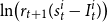 $\ln \!\big (r_{t+1}(s_t^i-I_t^i)\big )$
, from a non-pecuniary component tied to entrepreneurial success,
 $p_t \left(R^E_{t+1} \right)^\alpha$
. This reduced-form formulation is related to (but distinct from) the way non-pecuniary entrepreneurial motives are typically modeled in the empirical literature. In particular, Hurst and Pugsley (Reference Hurst and Pugsley2015) and Jones and Pratap (Reference Jones and Pratap2020) rationalize entrepreneurial choices by augmenting standard utility from consumption (or income) with a direct non-pecuniary payoff from operating one’s own business.Footnote 5 Our approach differs in that we do not introduce an additive taste shifter; instead, we represent these motives in reduced form by allowing entrepreneurial success to enter utility with convex curvature,
 $p_t\left(R^E_{t+1} \right)^\alpha$
. This delivers similar qualitative implications—entrepreneurship can be attractive even when expected pecuniary returns are modest—while remaining tractable for our general equilibrium analysis of buyouts and portfolio concentration.
The key curvature implications of (2) are that the objective is concave in the safe component and convex in the entrepreneurial payoff. Specifically, the safe term
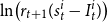 $\ln \!\big (r_{t+1}(s_t^i-I_t^i)\big )$
is concave in
 $I_t^i$
(reflecting increasing marginal opportunity costs of diverting resources away from safe saving), whereas the entrepreneurial-success term is convex in
 $R^E_{t+1}$
when
 $\alpha \gt 1$
.Footnote 6
Separability between the safe and entrepreneurial components is important for our mechanism and comparative statics because it enables a clean comparison of marginal returns to risky versus safe investment across the wealth distribution. In particular, the marginal utility cost of increasing entrepreneurial investment through the safe term is
 \begin{equation*} \frac {\partial }{\partial I_t^i}\ln \!\big (r_{t+1}(s_t^i-I_t^i)\big ) \;=\; -\frac {1}{s_t^i-I_t^i}, \end{equation*}
which decreases in wealth
 $s_t^i$
. Thus, for high-income the marginal value of allocating an additional unit to safe investment is relatively lower, making it more likely that the marginal gain from entrepreneurial exposure—operating through
 $p_t'(I_t^i)\left(R^E_{t+1} \right)^\alpha$
—dominates. The combination of (i) separability between safe and entrepreneurial components and (ii) convex utility in the entrepreneurial payoff predicts increasing portfolio concentration in risky private investments with wealth: as safe marginal utility declines with wealth, high-wealth agents should optimally tilt toward fewer, larger, and more concentrated positions in entrepreneurial assets.Footnote 7
2.2 Production
The final good, serving as the numeraire in the economy, is produced through combining labor with a diverse range of intermediate goods. The production technology follows a constant returns to scale specification:
 \begin{equation} Y_t=\frac {1}{1-\zeta }\left (\int _{0}^{N_t}x_{it}^{1-\zeta }di\right )L_t^\zeta ,\quad \zeta \in (0,1) \end{equation}
where
 $x_{it}$
represents the quantity of intermediate good
 $i$
utilized in production, while
 $L_t$
denotes the aggregate labor input.
Under the labor market equilibrium condition where
 $L_t=L\overline {e}$
, we can derive the inverse demand functions for intermediate goods along with the competitive wage rate. The price of intermediate good
 $i$
responds to its quantity according to:
 \begin{equation} q_{it} = x_{it}^{-\zeta }(L\overline {e})^\zeta \end{equation}
while the wage rate determination incorporates all intermediate goods:
 \begin{equation} w_t = \frac {\zeta }{1-\zeta }\left (\int _{0}^{N_t}x_{it}^{1-\zeta }di\right )(L\overline {e})^{\zeta -1} \end{equation}
The economy features two distinct regimes for intermediate goods production. For existing varieties indexed
 $i\in [0, N_{t-1}]$
, production occurs competitively with a one-to-one transformation from capital goods that fully depreciate each period. The supply function for these established varieties takes the form:
 \begin{equation} x_{it}=\left (\frac {1}{r_t}\right )^{1/\zeta }L\overline {e} \end{equation}
In contrast, newly invented varieties indexed
 $i\in (N_{t-1}, N_t]$
benefit from one-period patent protection, granting inventors temporary monopoly power. The optimal supply decision for patent holders yields:
 \begin{equation} x_{it}=\left (\frac {1-\zeta }{r_t}\right )^{1/\zeta }L\overline {e} \end{equation}
This monopolistic supply generates profits for each new variety inventor, with the profit flow given by:
 \begin{equation} R^E_t=\zeta \left (\frac {1-\zeta }{r_t}\right )^{(1-\zeta )/\zeta }L\overline {e} \end{equation}
Combining these elements, the economy’s factor price frontier emerges as:
 \begin{equation} w_t^{\zeta }r_t^{1-\zeta } =\left \{\frac {\zeta }{1-\zeta }\left [N_{t-1}+(N_t-N_{t-1})(1-\zeta )^{(1-\zeta )/\zeta }\right ]\right \}^\zeta \end{equation}
2.3 Initial conditions
The economy commences with specific initial conditions. A continuum of old agents of measure
 $L$
exists, each endowed with
 $k_1$
units of the capital good. These agents supply their entire capital endowment in the first period, after which the capital fully depreciates and the agents exit the economy. Notably, the model assumes no innovation occurs in the initial period, maintaining the variety count constant at
 $N_1=N_0=N\gt 0$
.
2.4 Optimization under self-sufficiency
First, consider optimization when there is no match between well-endowed and under-endowed agents.
2.4.1 Well-endowed agents
Since well-endowed agents do not possess business ideas, they face a standard consumption-savings problem subject to the constraints
 $0 \lt s^w_t \lt w_te^w$
and
 $I^w_t = 0$
. Their optimization problem is:
 \begin{equation*} \max _{s^w_t, I^w_t}{\ln} (w_te^w-s^w_t) + \beta \ln r_{t+1}(s^w_t-I^w_t) \end{equation*}
The solution yields optimal savings with no entrepreneurial investment:
 \begin{eqnarray} (s^w_t, I^w_t)=\left [\frac {\beta w_t e^w}{1+\beta }, 0\right ]. \end{eqnarray}
The corresponding indirect utility is:
 \begin{equation} u^{wr}_t=(1+\beta )\ln w_te^w+\beta \ln r_{t+1}-\ln \frac {(1+\beta )^{1+\beta }}{\beta ^\beta }. \end{equation}
2.4.2 Under-endowed agents
Under-endowed agents with business ideas solve a more complex problem subject to
 $0 \lt s^u_t \lt w_te^u$
and
 $0 \le I^u_t \lt s^u_t$
. Their decision depends on wage levels as shown in Lemma 1.
Lemma 1. The under-endowed agents’ optimal
 $(s^u_t, I^u_t)$
choices follow two regimes: (a) When
 $w_t \leq 1/p e^u$
:
 \begin{equation} \left(s^u_t, I^u_t \right) = \left [\frac {\beta w_t e^u}{1+\beta }, 0\right ] \end{equation}
(b) When
 $w_t \gt 1/p e^u$
:
 \begin{eqnarray} \left(s^u_t, I^u_t \right)=\left \{ \begin{array}{cl} \displaystyle \left [\frac {(I^u_t)^*+\beta w_t e^u}{1+\beta }, (I^u_t)^*\right ] & \mbox{if $0\le r_{t+1}\le r^u(w_t)$}\\[13pt] \displaystyle \left [\frac {\beta w_t e^u}{1+\beta }, 0\right ] & \mbox{if $r^u(w_t)\le r_{t+1}$} \end{array} \right . \end{eqnarray}
where the optimal investment is:
 \begin{equation} (I^u_t)^* = \frac {2w_t e^u}{1 + \sqrt {1 + \frac {4w_t e^u (1+\beta )}{\beta \left(R^E_{t+1} \right)^\alpha }}} \end{equation}
and
 $r^u(w_t)$
is a continuously increasing function of
 $w_t\ ({\in} [1/pe^u,+\infty ))$
with
 $r^u(1/pe^u)=0$
defined implicitly by:
 \begin{eqnarray} \ln \left [1-\frac {(I^u_t)^*}{w_t e^u}\right ]+\frac {\beta }{1+\beta }\left [p-\frac {1}{(I^u_t)^*}\right ]\left(R^E_{t+1} \right)^\alpha =0. \end{eqnarray}
Proof. See Appendix A.
The indirect utility differs by case. When no entrepreneurship occurs (
 $w_t \leq 1/p e^u$
or
 $r^u(w_t) \leq r_{t+1}$
):
 \begin{equation} u^{ur}_t=(1+\beta )\ln w_te^u+\beta \ln r_{t+1}-\ln \frac {(1+\beta )^{1+\beta }}{\beta ^\beta }; \end{equation}
With entrepreneurship (
 $w_t \gt 1/p e^u$
and
 $0 \leq r_{t+1} \leq r^u(w_t)$
):
 \begin{eqnarray} \begin{array}{r} \displaystyle u^{ur}_t=(1+\beta ) \,{\ln} [w_te^u-(I^u_t)^*]+\beta \left [p-\frac {1}{(I^u_t)^*}\right ]\left(R^E_{t+1} \right)^\alpha \\[12pt] \displaystyle +\beta \ln r_{t+1}-\ln \frac {(1+\beta )^{1+\beta }}{\beta ^\beta }. \end{array} \end{eqnarray}
These indirect utilities serve as threat points in the Nash bargaining analysis. Moreover, note that the curvature of the reservation utility in
 $R^E_{t+1}$
is regime-dependent. Only in the entrepreneurial regime—that is, when
 $w_t\gt 1/(pe^u)$
and
 $0\le r_{t+1}\lt r^u(w_t)$
—does the under-endowed agent choose a strictly positive entrepreneurial investment
 $(I_t^u)^*\gt 0$
.Footnote 8 In that region, the indirect utility
 $u_t^{ur}$
is strictly convex in the entrepreneurial payoff
 $R^E_{t+1}$
. The reason is that, by the envelope theorem, changes in
 $R^E_{t+1}$
affect the value function only through the direct term
 $\beta \big (p-1/(I_t^u)^*\big )\left(R^E_{t+1} \right)^\alpha$
, while the induced changes in the optimal choice
 $(I_t^u)^*$
do not enter the derivative.Footnote 9 Intuitively, this convexity becomes relevant only when income is high enough for entrepreneurship to be feasible and privately optimal.
2.5 Nash bargaining
When a well-endowed agent matches with an under-endowed agent to implement a business idea, their agreement solves the following optimization problem:
 \begin{equation*} \max _{\substack {s^w_t, s^u_t, \ I^w_t, I^u_t, R^w_{t+1}}} {\ln} (w_te^w-s^w_t) + \beta \left [\ln r_{t+1}(s^w_t-I^w_t) + \left (p-\frac {1}{I^w_t+I^u_t}\right )(R^w_{t+1})^\alpha \right ] \end{equation*}
subject to the participation constraint for under-endowed agents:
 \begin{equation} {\ln} (w_te^u-s^u_t) + \beta \left [\ln r_{t+1}(s^u_t-I^u_t) + \left (p-\frac {1}{I^w_t+I^u_t}\right )(R^E_{t+1}-R^w_{t+1})^\alpha \right ] = u^{ur}_t \end{equation}
and the limited liability condition:
 \begin{equation} 0 \le R^w_{t+1} \le R^E_{t+1} \end{equation}
where
 $R^w_{t+1}$
represents the well-endowed agent’s profit share. Two crucial features characterize this bargaining solution. First, the participation constraint implies that under-endowed agents receive exactly their reservation utility
 $u^{ur}_t$
, reflecting their lack of bargaining power. This outcome stems from competition among the measure
 $(1-2\theta )L$
of unmatched under-endowed agents who could potentially make better offers.Footnote 10 Second, the optimal profit allocation
 $R^w_{t+1}$
equals
 $R^E_{t+1}$
when solutions exist, as
 $\alpha \gt 1$
implies corner solutions and
 $R^w_{t+1} = 0$
would leave well-endowed agents no better off than autarky.
The problem can be reformulated using the variable transformations
 $\tilde {s}^w_t \equiv s^w_t + I^u_t$
,
 $\tilde {s}^u_t \equiv s^u_t - I^u_t$
,
 $\tilde {I}^w_t \equiv I^w_t + I^u_t$
, and
 $a_t \equiv -I^u_t$
:
 \begin{equation*} \max _{\tilde {s}^w_t, \tilde {s}^u_t, \tilde {I}^w_t, a_t} {\ln} (w_te^w-a_t-\tilde {s}^w_t) + \beta \left [\ln r_{t+1}(\tilde {s}^w_t-\tilde {I}^w_t) + \left (p-\frac {1}{\tilde {I}^w_t}\right )\left(R^E_{t+1} \right)^\alpha \right ] \end{equation*}
subject to:
 \begin{equation} {\ln} (w_te^u + a_t - \tilde {s}^u_t) + \beta \ln r_{t+1}\tilde {s}^u_t = u^{ur}_t \end{equation}
The solution yields optimal policies:
 \begin{align} \tilde {s}^u_t &= \frac {\beta (w_t e^u + a_t)}{1+\beta } \\[-10pt] \nonumber \end{align}
 \begin{align} \tilde {s}^w_t &= \frac {\tilde {I}^w_t + \beta (w_t e^w - a_t)}{1+\beta }\\[-10pt] \nonumber \end{align}
 \begin{align} \tilde {I}^w_t &= \frac {2(w_t e^w - a_t)}{1 + \sqrt {1 + \frac {4(1+\beta )(w_t e^w - a_t)}{\beta \left(R^E_{t+1} \right)^\alpha }}}\\[7pt] \nonumber \end{align}
Lemma 2. For
 $\theta \lt 1/2$
, the optimal transfer
 $a_t$
follows: (a) When
 $w_t \le 1/p e^u$
or when
 $w_t \gt 1/p e^u$
and
 $r^u(w_t) \le r_{t+1}$
:
 \begin{equation} a_t = 0 \end{equation}
(b) When
 $w_t \gt 1/p e^u$
and
 $0 \le r_{t+1} \le r^u(w_t)$
:
 \begin{equation} a_t=\left [w_t e^u-(I^u_t)^*\right ]\exp \left \{\frac {\beta }{1+\beta }\left [p-\frac {1}{(I^u_t)^*}\right ]\left(R^E_{t+1} \right)^\alpha \right \}-w_te^u, \end{equation}
where
 $(I^u_t)^*$
and
 $r^u(\! \cdot \!)$
are defined in Lemma 1.
Proof. See Appendix A.
Substituting these results into the optimal policies reveals that well-endowed agents minimize idea acquisition costs, sometimes obtaining business ideas for free when condition equation (24) holds. This outcome reflects the competitive pressure from unmatched under-endowed agents in the market for ideas.
3. Temporary equilibrium
The temporary equilibrium in period
 $t \geq 2$
depends on the entrepreneurial activities in period
 $t-1$
. We characterize equilibria through three distinct regimes based on the composition of innovators in the previous period.Footnote 11
3.1 Equilibrium characterization
The capital market clears when aggregate demand
 $K_t^D$
equals aggregate supply
 $K_t^S$
. Capital demand comprises the capital required for producing both established and new intermediate goods:
 \begin{equation} K_t^D = N_{t-1}\left (\frac {1}{r_t}\right )^{1/\zeta }L\overline {e} + (N_t-N_{t-1})\left (\frac {1-\zeta }{r_t}\right )^{1/\zeta }L\overline {e}. \end{equation}
Capital supply originates from the net savings of the young cohort born in period
 $t-1$
:
 \begin{equation*} K_t^S = \theta L \cdot (s_{t-1}^{w}-I^w_{t-1}) + (1-\theta ) L \cdot (s_{t-1}^{u} - I_{t-1}^{u}). \end{equation*}
Using the optimal savings policies
 $s_{t-1}^i-I_{t-1}^i = \frac {\beta }{1+\beta }(w_{t-1}e^i-I^i_{t-1})$
for
 $i = u, w$
, we obtain the aggregate capital supply:
 \begin{equation} K_t^S = \frac {\beta }{1+\beta }\left [w_{t-1}\overline {e} - \mathcal{I}_{t-1}\right ]L, \end{equation}
where
 $\mathcal{I}_{t-1} = \theta \cdot I_{t-1}^w + (1-\theta ) \cdot I_{t-1}^u$
, varies across three regimes:
-
(a) No entrepreneurship:
 $\mathcal{I}_{t-1} = 0$
and
$N_t = N_{t-1}$
.
-
(b) Under-endowed only:
$\mathcal{I}_{t-1} = (1-\theta )(I^u_{t-1})^*$
with new varieties:(28)
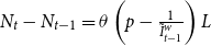
\begin{equation} N_t - N_{t-1} = (1-\theta )\left [p-\frac {1}{(I^u_{t-1})^*}\right ]L. \end{equation}
-
(c) Matched pairs (
$\theta \lt 1/2$
): The composition of entrepreneurial investment depends on whether unmatched under-endowed agents find independent innovation optimal under the equilibrium interest rate yield by this regime. When
$r_t \leq r^u(w_{t-1})$
:(29)with new variety creation:
\begin{equation} \mathcal{I}_{t-1} = \theta \tilde {I}^w_{t-1} + (1-2\theta )(I^u_{t-1})^*, \end{equation}
(30)Otherwise, only matched pairs innovate:
\begin{equation} N_t - N_{t-1} = \left [\theta \left (p-\frac {1}{\tilde {I}^w_{t-1}}\right ) + (1-2\theta )\left (p-\frac {1}{(I^u_{t-1})^*}\right )\right ]L. \end{equation}
$\mathcal{I}_{t-1} = \theta \tilde {I}^w_{t-1}$
and
$N_t - N_{t-1} = \theta \left (p-\frac {1}{\tilde {I}^w_{t-1}}\right )L$
.


3.2 Market clearing conditions
Each regime yields a distinct market-clearing condition:
(a) No entrepreneurship:
 \begin{equation} N_{t-1}\left (\frac {1}{r_t}\right )^{1/\zeta } = \frac {\beta }{1+\beta }w_{t-1}. \end{equation}
(b) Under-endowed only:
 \begin{equation} N_{t-1}\left (\frac {1}{r_t}\right )^{1/\zeta } + (1-\theta )\left [p-\frac {1}{(I^u_{t-1})^*}\right ]\left (\frac {1-\zeta }{r_t}\right )^{1/\zeta }L = \frac {\beta }{1+\beta }\left [w_{t-1} - (1-\theta )\frac {(I^u_{t-1})^*}{\overline {e}}\right ]. \end{equation}
(c) Matched pairs: When unmatched under-endowed agents innovate independently:
 \begin{equation} N_{t-1}\left (\frac {1}{r_t}\right )^{1/\zeta } + (N_t-N_{t-1})\left (\frac {1-\zeta }{r_t}\right )^{1/\zeta }L = \frac {\beta }{1+\beta }\left [w_{t-1} - \frac {\theta \tilde {I}^w_{t-1} + (1-2\theta )(I^u_{t-1})^*}{\overline {e}}\right ]. \end{equation}
where
 $N_t-N_{t-1}$
is given in equation (30). Otherwise:
 \begin{equation} N_{t-1}\left (\frac {1}{r_t}\right )^{1/\zeta } + (N_t-N_{t-1})\left (\frac {1-\zeta }{r_t}\right )^{1/\zeta }L = \frac {\beta }{1+\beta }\left [w_{t-1} - \frac {\theta \tilde {I}^w_{t-1} }{\overline {e}}\right ]. \end{equation}
and
 $N_t - N_{t-1} = \theta \left (p-\frac {1}{\tilde {I}^w_{t-1}}\right )L$
.
In each regime
 $j \in \{(a),(b),(c)\}$
, substituting the regime-specific investment rules into the corresponding capital market-clearing condition yields an excess-demand function
 $E_{t-1}^j(r_{t})$
in the single unknown
 $r_{t}$
. For fixed
 $(N_{t-1},w_{t-1})$
and parameters, individual investment rules are continuous in
 $(r_{t+1}, R^E_{t+1})$
and strictly decreasing in
 $r_{t}$
, whereas incremental variety
 $N_t-N_{t-1}$
is either
 $0$
or strictly decreasing in
 $r_{t}$
. It follows that, within each regime,
 $E_{t-1}^j(r_{t})$
is continuous and strictly decreasing in
 $r_{t}$
and therefore admit at most one solution to
 $E_{t-1}^j(r_{t})=0$
. In Section 6, we provide an algorithm to pin down the temporary equilibrium and simulate the transition path.
4. Long-run economic states
The economy can converge to three distinct long-run states, each characterized by different patterns of innovation and financial contracts. These states emerge endogenously from the model’s dynamics and have markedly different implications for growth trajectories.
4.1 No-innovation steady state
In this stagnant equilibrium, the variety of intermediate goods stabilizes at some finite level
 $\overline {N}$
. The economy reaches a stationary configuration where two key relationships govern factor prices. First, the factor price frontier simplifies to a static relationship between normalized wages and interest rates:
 \begin{equation} \left (\frac {\overline {w}}{\overline {N}}\right )^\zeta \overline {r}^{1-\zeta } = \left (\frac {\zeta }{1-\zeta }\right )^\zeta \end{equation}
Second, capital market clearing imposes a direct connection between these variables:
 \begin{equation} \left (\frac {1}{\overline {r}}\right )^{1/\zeta } = \frac {\beta }{1+\beta }\frac {\overline {w}}{\overline {N}} \end{equation}
These conditions jointly pin down the steady-state values of the interest rate and the wage-to-variety ratio:
 \begin{equation} \overline {r} = \frac {1+\beta }{\beta }\cdot \frac {1-\zeta }{\zeta }, \quad \frac {\overline {w}}{\overline {N}} = \left (\frac {\beta }{1+\beta }\right )^{(1-\zeta )/\zeta } \left (\frac {\zeta }{1-\zeta }\right )^{1/\zeta } \end{equation}
Whether the economy reaches this state depends crucially on initial conditions. When the initial variety of goods
 $N_0$
exceeds a critical threshold
 $\overline {N}^*$
, convergence to this stagnant equilibrium becomes impossible, as established in the next lemma:
Lemma 3. Let
 $\overline {w}$
,
 $\overline {N}$
, and
 $A$
be, respectively, the values of
 $w_t$
,
 $N_t$
, and
 $w_t/N_t$
in the state of no-innovation. Then, there is a positive constant
 $\overline {N}^*$
such that
 \begin{eqnarray} \overline {N}\le \overline {N}^* \qquad \mbox{and} \qquad \overline {w}\le A\overline {N}^*. \end{eqnarray}
Proof. See Appendix A.
4.2 Sustained innovation without buyouts
When innovation persists exclusively through under-endowed entrepreneurs, the economy exhibits several characteristic growth patterns. The variety of intermediate goods grows without bound, with
 $N_t \to \infty$
as
 $t \to \infty$
. Despite this growth, the share of income that entrepreneurs devote to innovation expenditures vanishes asymptotically, with
 $(I_t^u)^*/w_t \to 0$
.
The economy settles into a balanced growth path where the long-run growth rate tends to zero, and factor prices maintain stable relationships. The interest rate converges to the same value found in the stagnant equilibrium:
 \begin{equation} \lim _{t\to \infty } r_t = \frac {1+\beta }{\beta }\cdot \frac {1-\zeta }{\zeta } \end{equation}
while the wage-to-variety ratio approaches:Footnote 12
 \begin{equation} \lim _{t\to \infty } \frac {w_t}{N_t} = \left (\frac {\beta }{1+\beta }\right )^{(1-\zeta )/\zeta } \left (\frac {\zeta }{1-\zeta }\right )^{1/\zeta } \end{equation}
Entrepreneurial participation remains optimal throughout this growth path because the expected returns to innovation stay positive (consider the limit of the LHS of (15)).
4.3 Sustained innovation with buyouts
The economy with active buyouts exhibits similar asymptotic properties, including unbounded growth in matched entrepreneurial investment, declining relative investment shares despite absolute growth, and convergence of monopoly profits to a finite steady-state value:
 \begin{align} &\lim _{t\to +\infty }\tilde {I}^w_t=+\infty \\[-10pt] \nonumber \end{align}
 \begin{align} &\lim _{t\to +\infty }\tilde {I}^w_t/w_t=0 \\[-10pt] \nonumber \end{align}
 \begin{align} \lim _{t\to +\infty }R^E_{t+1}&=\zeta ^{1/\zeta }\left (\frac {\beta }{1+\beta }\right )^{(1-\zeta )/\zeta }L\overline {e}\equiv R^E \\[10pt] \nonumber \end{align}
The limiting conditions equations (39), (40), and
 $(I_t^u)^*/w_t \to 0$
continue to hold in this regime. To analyze the capital market equilibrium, we transform equation (33) into:
 \begin{equation} \begin{aligned} &\left [\left (\frac {1}{r_t}\right )^{1/\zeta }-\frac {\beta }{1+\beta }\cdot \frac {w_{t-1}}{N_{t-1}}\right ]\overline {e}\\[3pt] &+\left \{\theta \left (p-\frac {1}{\tilde {I}^w_{t-1}}\right )+(1-2\theta )\left [p-\frac {1}{(I^u_{t-1})^*}\right ]\right \}\left (\frac {1-\zeta }{r_t}\right )^{1/\zeta }\frac {L\overline {e}}{N_{t-1}}\\[3pt] &+\frac {\beta }{1+\beta }\left [\theta \frac {\tilde {I}^w_{t-1}}{N_{t-1}}+(1-2\theta )\frac {(I^u_{t-1})^*}{N_{t-1}}\right ]=0. \end{aligned} \end{equation}
As
 $t\to +\infty$
, this equation simplifies considerably. The convergence results
 $(I_t^u)^*/w_t \to 0$
,
 $(I_t^w)^*/w_t \to 0$
, equation (40) collectively ensure that the second and third terms vanish asymptotically, leaving:
 \begin{equation} \lim _{t\to +\infty }\left [\left (\frac {1}{r_t}\right )^{1/\zeta }-\frac {\beta }{1+\beta }\cdot \frac {w_{t-1}}{N_{t-1}}\right ]\overline {e}=0. \end{equation}
This limiting condition reproduces the same interest rate and wage-to-variety ratio relationships established in the no-buyout case.
The optimal transfer amount
 $a_t$
between agents exhibits important asymptotic behavior. Rewriting equation (25) as:
 \begin{eqnarray} \frac {a_t}{w_t e^u}=\left [1-\frac {(I^u_t)^*}{w_t e^u}\right ]\exp \left \{\frac {\beta }{1+\beta }\left [p-\frac {1}{(I^u_t)^*}\right ]\left(R^E_{t+1} \right)^\alpha \right \}-1. \end{eqnarray}
and combining with the limits, we obtain
 \begin{equation} \lim _{t\to +\infty }\frac {a_t}{w_t e^u}=\exp \left \{\frac {\beta }{1+\beta }p(R^E)^\alpha \right \}-1 \end{equation}
which implies unbounded growth in absolute transfer amounts:
 \begin{equation} \lim _{t\to +\infty }a_t=+\infty . \end{equation}
The well-endowed agents’ buyout decision depends on comparing the utility from purchasing ideas:
 \begin{equation*} (1+\beta )\ln (w_t e^w-a_t-\tilde {I}^w_t)+\beta \ln r_{t+1}+\beta \left (p-\frac {1}{\tilde {I}^w_t}\right )\left(R^E_{t+1} \right)^\alpha -\frac {(1+\beta )^{1+\beta }}{\beta ^\beta } \end{equation*}
with their reservation utility from equation (11). The participation condition simplifies asymptotically to:
 \begin{equation} \ln \left (1-\frac {a_t+\tilde {I}^w_t}{w_t e^w}\right )+\frac {\beta }{1+\beta }\left (p-\frac {1}{\tilde {I}^w_t}\right )\left(R^E_{t+1} \right)^\alpha \ge 0 \end{equation}
which converges to the key inequality:
 \begin{equation*} \ln \left \{1-\frac {e^u}{e^w}\left [\exp \left (\frac {\beta }{1+\beta }p(R^E)^\alpha \right )-1\right ]\right \}+\frac {\beta }{1+\beta }p(R^E)^\alpha \ge 0 \end{equation*}
This leads to our central existence result:
Proposition 1. In an economy with sustained innovation, buyout emerges if and only if
 \begin{equation*} \frac {e^w}{e^u}\gt \exp \left [\frac {\beta }{1+\beta }p(R^E)^\alpha \right ]. \end{equation*}
Proof. The necessity follows from the asymptotic analysis above. For sufficiency, when the condition holds, equations (49) are satisfied for sufficiently large
 $t$
, ensuring mutually beneficial idea transfers between agent types.
Proposition 1 establishes that persistent buyouts emerge if and only if the endowment ratio
 $e^w/e^u$
exceeds a critical threshold. The threshold is jointly determined by the success probability
 $p$
, the intensity of non-pecuniary utility
 $\alpha$
, the discount factor
 $\beta$
, and the steady-state entrepreneurial return
 $R^E$
. These parameters influence the persistence of buyout activity through two distinct channels. First, higher values of
 $p$
,
 $\alpha$
,
 $\beta$
, or
 $R^E$
increase the acquisition price required to compensate under-endowed agents for their forgone entrepreneurial utility, as shown in the asymptotic transfer condition equation (47). This reflects the fact that when entrepreneurial success is more likely, future profits are more valuable, or agents derive greater non-pecuniary benefits from entrepreneurship, idea holders demand higher compensation to relinquish control. Second, these same parameters simultaneously affect wealthy agents’ willingness to pay for entrepreneurial participation. Higher values enhance the non-pecuniary utility wealthy agents derive from implementing business ideas, potentially increasing their reservation acquisition prices. Consequently, economies require greater initial inequality to sustain buyout activity when entrepreneurial prospects are more attractive.
5. Buyout funds and economic growth
In the model, entrepreneurship provides intrinsic utility to idea holders, while affluent agents value the experience of implementing businesses enough to pay premiums that make transfers mutually beneficial. This mechanism captures empirical observations that private equity participation is often driven by non-pecuniary motives as well as financial returns and has important implications for inequality and economic growth.
5.1 Buyout and growth
Buyouts affect innovation and variety expansion through two complementary channels. First, buyouts reallocate projects to agents with greater effective resources, increasing per-project success probabilities and accelerating the introduction of new intermediate goods. Without buyouts, only under-endowed idea owners implement projects and variety growth is
 \begin{equation} \Delta N_t^{\text{no-buyout}} = (1-\theta )\left (p - \frac {1}{(I_{t-1}^u)^*}\right )L. \end{equation}
where
 $(I_{t-1}^u)^*$
is the optimal investment of an under-endowed implementer. With active buyouts, transferred ideas are implemented by well-endowed agents who invest
 $\tilde {I}_{t-1}^w$
, while the remaining unmatched under-endowed agents also begin businesses, so
 \begin{equation} \Delta N_t^{\text{buyout}} = \left [\theta \left (p - \frac {1}{\tilde {I}_{t-1}^w}\right ) + (1-2\theta )\left (p - \frac {1}{(I_{t-1}^u)^*}\right )\right ]L. \end{equation}
In our setup, both investment choices can be written as
 $I(x)$
evaluated at different effective resources,
 \begin{equation*} (I_{t-1}^u)^* = I(w_{t-1}e^u),\qquad \tilde {I}_{t-1}^w = I(w_{t-1}e^w - a_{t-1}), \end{equation*}
with
 \begin{equation*} I(x) = \frac {2x}{1+\sqrt {1+\dfrac {4(1+\beta )x}{\beta (R_t^E)^\alpha }}},\quad x\gt 0. \end{equation*}
Since
 $I'(x)\gt 0$
for all
 $x\gt 0$
, larger effective resources raise investment and hence the success probability. Under the buyout persistence condition,
 \begin{equation*} \frac {e^w}{e^u} \gt \exp \!\left \{\frac {\beta }{1+\beta }p(R^E)^\alpha \right \}, \end{equation*}
and the associated asymptotic transfer rule
 \begin{equation*} \lim _{t\to \infty }\frac {a_t}{w_t e^u} = \exp \!\left \{\frac {\beta }{1+\beta }p(R^E)^\alpha \right \}-1, \end{equation*}
we have for large
 $t$
, that
 \begin{equation*} w_t e^w - a_t \gt w_t e^u. \end{equation*}
hence
 $\tilde {I}_t^w \gt (I_t^u)^*$
and
 \begin{equation*} p - \frac {1}{\tilde {I}_t^w} \gt p - \frac {1}{(I_t^u)^*}. \end{equation*}
Thus, reallocating projects to wealthier implementers raises the per-project success probability and accelerates the short-run introduction of intermediate goods.Footnote 13
Second, when
 $\theta \lt 1/2$
(the empirically relevant case where capital-abundant agents are fewer), a trickle-down effect emerges on the extensive margin. Initially, many under-endowed agents lack the resources to implement ideas, and growth is approximately
 $\theta Lp$
varieties per period. As matched (buyout-implemented) innovations expand the variety of intermediates and push up wages, previously constrained under-endowed agents acquire the means to launch their own projects. When the
 $(1-2\theta )L$
previously inactive under-endowed agents become active, variety growth increases to the expression given for
 $\Delta N_t^{\text{no-buyout}}$
. Over time, wages and investments rise, and both success probabilities approach
 $p$
, and long-run variety growth in either regime converges to
 $(1-\theta )Lp$
.
These channels are consistent with the institutional view that buyouts are not merely a relabeling of ownership, but involve concentrated control rights and active governance and operational restructuring of portfolio companies (Kaplan and Stromberg, Reference Kaplan and Stromberg2009). Moreover, using industry-level evidence, Bernstein et al. (Reference Bernstein, Lerner, Sorensen and Strömberg2017) find that private equity activity predicts subsequent improvements in industry performance, in line with our mechanism, which reallocates ownership to better-capitalized (and more actively involved) owners, thereby raising effective investment and innovation outcomes.
5.2 Policy implications
The model yields a nuanced set of policy implications that depend on the economy’s stage of development. In settings where under-endowed agents are initially unable to implement projects independently, some concentration of resources can play a constructive role: wealthy agents, motivated both by returns and non-pecuniary gains, provide upfront resources and acquisition premia that bring latent ideas to market. In such early-stage contexts, blunt policies that substantially raise the effective cost of private capital (e.g., by sharply increasing taxation on active investment without compensating measures) risk suppressing a private channel that jump-starts innovation. As the economy develops, endogenous wage increases improve the outside options of idea holders and reduce the social necessity of buyouts. At this intermediate stage, policies that broaden credit access or offer targeted support to nascent entrepreneurs (subsidized lending, matching grants, or public seed equity) can accelerate the shift from buyout-mediated commercialization to broad-based independent entrepreneurship.
Tax and fiscal design have ambiguous effects: lower taxes on returns to active investment raise wealthy agents’ willingness to bid for projects and may foster buyouts where they would otherwise be absent, whereas redistributive policies reduce wealthy agents’ capacity to pay acquisition premia while simultaneously strengthening under-endowed agents’ ability to implement ideas. Regulatory choices that affect contractual forms (earn-outs, equity retention) and market structure also matter: contracts that better share upside with originators can reduce required upfront premia and improve distributional outcomes without eliminating the matched improvement gains.
Taken together, these considerations suggest a stage-dependent policy strategy. In nascent or credit-constrained environments, preserving incentives for active, control-oriented investors can be growth-enhancing; as financial access widens, the policy emphasis should shift toward expanding independent entrepreneurship and ensuring that buyout activity—if present—operates under contractual and regulatory arrangements that align incentives and limit value extraction.Footnote 14 A full welfare assessment of these trade-offs requires quantitative extensions that embed taxes, subsidies, and alternative contracting into the calibrated model, which we leave for future work.
6. Numerical illustrations
This section implements the model numerically in four steps. Section 6.1 introduces a light-touch calibration that maps the key preference and technology parameters to simple empirical moments. Section 6.2 describes the algorithm used to compute temporary equilibria and transition paths under a given parameterization. Section 6.3 then uses this machinery to construct two benchmark transition paths that illustrate when buyouts disappear versus persist and quantifies the contribution of the two growth channels. Finally, Section 6.4 conducts a sensitivity analysis, showing how the buyout regimes move with the parameters that enter the inequality threshold derived in Proposition 1.
6.1 Parameterization
The numerical illustration follows a light-touch calibration strategy. We anchor the key heterogeneity and innovation parameters to simple moments from the wealth distribution and from evidence on venture-backed project quality. Table 1 summarizes the main parameters used in the simulations. Throughout, we normalize the endowment of under-endowed agents to one,
 $e^u=1$
, so that all monetary variables can be interpreted in units of the under-endowed agent’s period income
 $w_t e^u$
.
Baseline parameter values for the numerical illustration

Table 1. Long description
A table with 8 rows and 4 columns. The columns are labeled Symbol, Value, Description, and Discipline/source. The table summarizes baseline parameter values for a numerical illustration. Row 1: Symbol, e^u; Value, 1; Description, Endowment of under-endowed agents; Discipline/source, Normalization. Row 2: Symbol, e^w; Value, 7.64; Description, Endowment of well-endowed agents; Discipline/source, Top 10 percent wealth share. Row 3: Symbol, theta; Value, 0.10; Description, Population share of well-endowed agents; Discipline/source, Top 10 percent of the wealth distribution. Row 4: Symbol, p; Value, 0.21; Description, Success probability of a buyout-backed project; Discipline/source, The fraction of good projects. Row 5: Symbol, alpha; Value, 1.5; Description, Curvature of entrepreneurial thrill utility; Discipline/source, Moderate convexity. Row 6: Symbol, beta; Value, 0.985^30; Description, Subjective discount factor; Discipline/source, 30 years per generation. Row 7: Symbol, xi; Value, 2/3; Description, Labor share in production; Discipline/source, Standard. Row 8: Symbol, L; Value, 10; Description, Population size; Discipline/source, The scale of the economy.
We now briefly discuss how the key parameters linking the model to the data are chosen.
Inequality parameters
 $\theta$
and
 $(e^w,e^u)$
.
We interpret
 $\theta$
as the population share of “well-endowed” agents who are rich enough to finance buyouts. In the numerical exercises, we set
 $\theta = 0.10$
, corresponding to the top
 $10\%$
of the wealth distribution in advanced economies.
Given
 $\theta$
, we choose the ratio
 $e^w/e^u$
to mimic a simple moment of the empirical wealth distribution. In our two-type model, with
 $e^u$
normalized to one, the wealth share of well-endowed agents is
 \begin{equation*} s^{\text{model}}(\theta ,e^w) = \frac {\theta e^w}{\theta e^w + (1-\theta )e^u} = \frac {\theta e^w}{\theta e^w + (1-\theta )}. \end{equation*}
The World Inequality Database reports that the top
 $10\%$
hold roughly
 $42$
–
 $47\%$
of aggregate wealth in industrialized economies. This range implies an endowment ratio
 $e^w/e^u$
between about
 $6.52$
and
 $7.98$
in our two-type framework when
 $\theta =0.10$
and
 $e^u=1$
. In the numerical exercises, we set
 \begin{equation*} (e^w,e^u)=(7.64,1), \end{equation*}
so that
 \begin{equation*} s^{\text{model}}(0.10,7.64) = \frac {0.10\times 7.64}{0.10\times 7.64 + 0.90} = \frac {0.764}{1.664} \approx 0.459 . \end{equation*}
Thus, the implied wealth share of well-endowed agents is about
 $45.9\%$
, which lies well within the empirical range reported for the top decile. In this sense, the baseline parameterization captures a realistic degree of wealth inequality while using the value actually employed in the numerical simulations.
Success probability
 $p$
.
In the model,
 $p$
is the max probability that an implemented project yields a successful entrepreneurial payoff
 $R^E$
. To discipline its magnitude, we draw on Greenwood et al. (Reference Greenwood, Han and Sánchez2022), who sets the share of good ideas to
 $\rho = 0.21$
, implying that roughly
 $21\%$
of funded ventures are high-quality. We interpret this fraction as an empirical counterpart to the max success probability of a buyout-backed idea and therefore set
 $p = 0.21$
in our baseline simulations.
These choices provide a transparent benchmark for the dynamic experiments that follow. Given this baseline parameterization, we next describe how we compute equilibrium transition paths under different regimes.
6.2 Computation algorithm
Given the parameterization above, we compute the transition path
 $\{N_t, r_t, w_t, I_t^u, I_t^w\}_{t=1}^T$
by iterating on the temporary equilibrium problem for each
 $t$
, solving for
 $r_{t+1}$
, and classifying the regime. The algorithm proceeds as follows:
-
1. Initialization. Fix a horizon
$T$
, initial variety counts
$(N_0,N_1)$
, and an initial interest rate
$r_1$
. Set
$t=1$
. -
2. Factor prices. Given
$(N_{t-1},N_t,r_t)$
, compute the wage
$w_t$
from equation (9). For a candidate
$r_{t+1}$
, compute
$R^E_{t+1}(r_{t+1})$
from equation (8). -
3. Individual decisions. For the current candidate regime
$j\in \{(a),(b),(c)\}$
described in Section 3, use
$(w_t,r_{t+1},R^E_{t+1})$
and Lemma 1–2 to compute the corresponding investment and transfer decisions
$(I_t^u,I_t^w,\tilde I_t^w,a_t)$
and update
$N_{t+1}$
using equations (28)–(30). -
4. Capital market clearing. Plug these decisions into the appropriate capital market-clearing condition (31), (32), or (33) to construct
$E_t^j(r_{t+1})$
. Use a standard one-dimensional root-finding method to find the
$r_{t+1}$
such that
$E_t^j(r_{t+1})=0$
. -
5. Regime consistency and selection. Check that the regime-defining inequalities are satisfied: in particular, verify that under-endowed agents’ utility under the proposed contracts is at least as high as in autarky, and that well-endowed agents are willing to finance the stipulated buyouts. If regime
$j$
is not self-consistent, switch to another regime and repeat steps 3–4. In states where more than one regime is self-consistent, we select an equilibrium with active buyouts whenever both types strictly prefer it to the no-buyout outcome, focusing on the privately preferred equilibrium path among the regimes considered. -
6. Update. Record
$\{w_t,r_{t+1},I_t^u,I_t^w,\tilde I_t^w,a_t,N_{t+1}\}$
, set
$t\leftarrow t+1$
, and repeat until
$t=T$
.


The resulting simulated transition paths for wages, interest rates, investment, transfers, and varieties provide the basis for the numerical examples in the next subsection and for the sensitivity analysis in Section 6.4.
6.3 Numerical examples
With the baseline parameterization and computation algorithm in place, we now illustrate the model’s dynamics in two benchmark economies that differ in their degree of inequality. These examples are chosen to mirror the theoretical regimes characterized in the previous sections and to quantify the contributions of the matched improvement and extensive margin mechanisms to variety growth.
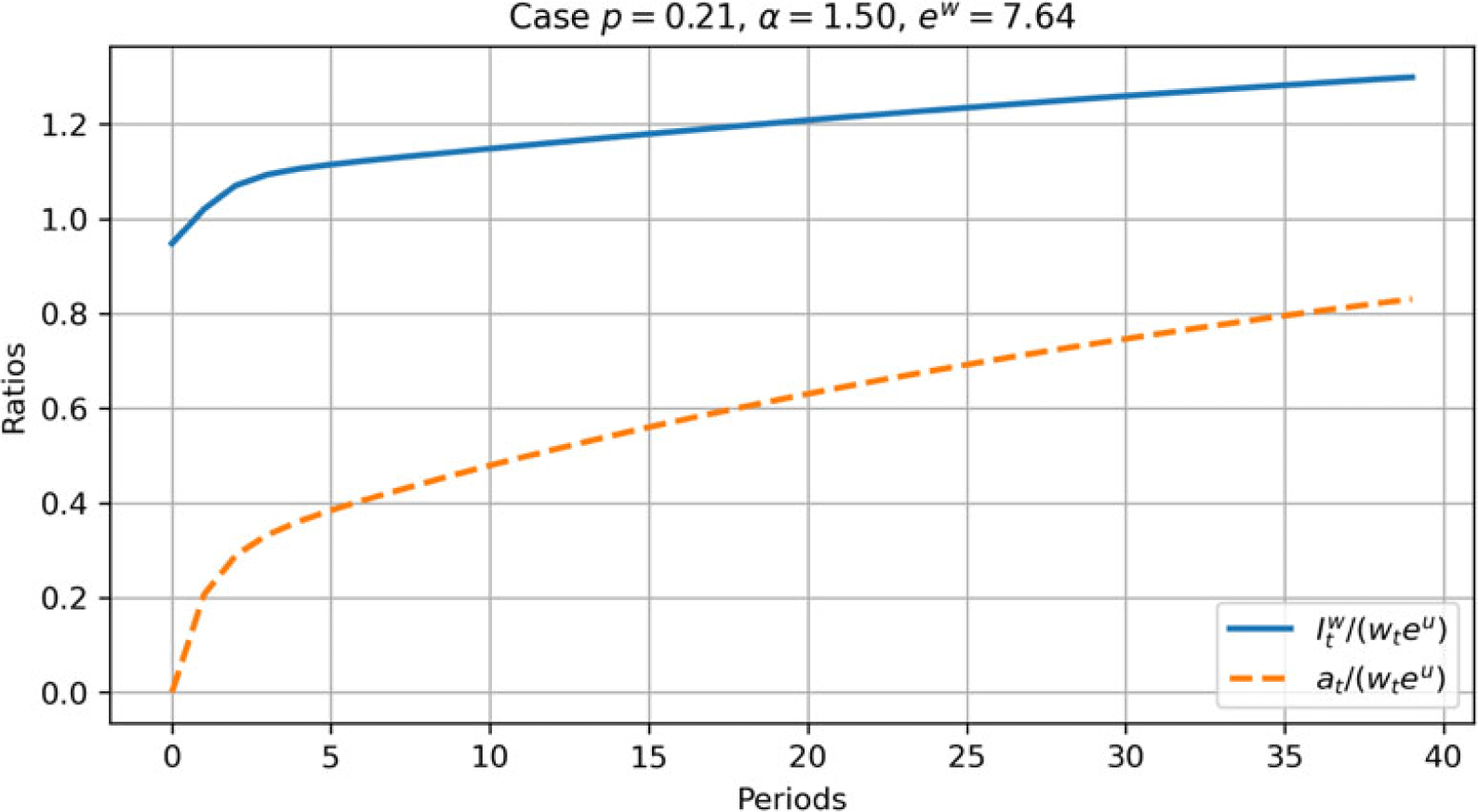
We first consider an economy in which buyouts initially emerge but eventually disappear. Figure 1 shows this scenario, which arises when Proposition 1’s condition fails and well-endowed agents are scarce. With initial parameters
 $(e^w,e^u)=(1.1,1)$
and
 $(N_1,r_1)=(30,5)$
, we observe three distinct phases. Early periods show no innovation due to low incomes (
 $I^w_t=a_t=0$
). As capital accumulation reduces interest rates and raises reservation utilities, under-endowed agents begin selling ideas at positive prices (
 $I^w_t\gt 0$
,
 $a_t\gt 0$
). The distance between the
 $I^w_t$
and
 $a_t$
lines represents total project commitment. Eventually, a kink emerges where well-endowed agents cease purchases (
 $I^w_t=0$
) and under-endowed agents implement ideas independently (
 $I^u_t=-a_t\gt 0$
), demonstrating how buyouts fade when endowment disparities are modest.
Dynamics of investment and transfers in an economy without persistent buyouts in the first 40 periods. Investment of well-endowed agents:
 $I^w_t/(w_t e^u)$
; transfer to under-endowed agents:
 $a_t/(w_t e^u)$
.

Table 2 reports the quantitative decomposition of variety growth in this disappearing-buyout case. During the 16-period buyout existence phase, the matched improvement channel (well-endowed agents raising project success probabilities) contributes 13.05% of new varieties, while the extensive margin channel (unmatched under-endowed agents entering entrepreneurship) accounts for 86.95%. In the long run, buyouts disappear entirely, leaving the extensive margin as the sole driver of growth (
 $\Delta N_{\text{buyout},t}=1.56$
, 100% from the extensive margin).
Growth mechanism decomposition for disappearing-buyout case (
 $e^w/e^u=1.1$
,
 $\theta =0.1$
)

Table 2. Long description
A table comparing growth mechanisms for disappearing-buyout case. The table has two columns: Buyout existence periods (n = 16) and Long-run (Last 200 periods). It has three rows labeled with metrics: Total new varieties, Matched pairs, and Extensive margin. Row 1: Total new varieties, 1.03, 1.56. Row 2: Matched pairs, 0.13 (13.05%), 0.00 (0.00%). Row 3: Extensive margin, 0.90 (86.95%), 1.56 (100.00%). The table shows that during the buyout existence periods, the matched pairs contribute 13.05% and the extensive margin contributes 86.95% to the total new varieties. In the long-run, the extensive margin alone drives the growth, contributing 100%.
Notes: Values in parentheses denote percentage contributions to
 $\Delta N_{\text{buyout},t}$
. Matched pairs channel:
 $\theta \cdot (p - 1/\tilde {I}^w_{t-1}) \cdot L$
; Extensive margin channel:
 $ (1-2\theta ) \cdot (p - 1/(I^{u}_{t-1})^* \cdot L)$
. Parameters:
 $p=0.21$
,
 $\alpha =1.5$
,
 $L=10$
. Total periods
 $T=800$
.
Growth mechanism decomposition for persistent buyout case (
 $e^w/e^u=7.64$
,
 $\theta =0.1$
)

Table 3. Long description
A table comparing the growth mechanism decomposition for a persistent buyout case during buyout existence periods and long-run periods. The table has three rows and three columns. Column headers are Metric, Buyout existence periods (n = 799), and Long-run (Last 200 periods). Row labels are Total new varieties, Matched pairs, and Extensive margin. Row 1: Total new varieties, 1.75, 1.81. Row 2: Matched pairs, 0.21 (11.94%), 0.21 (11.58%). Row 3: Extensive margin, 1.54 (88.06%), 1.60 (88.42%).
Notes: See Table 2 for variable definitions and parameters.
Dynamics of investment and transfers in an economy with persistent buyouts in the first 40 periods.

Figure 2 presents the contrasting case where Proposition 1’s condition holds with
 $(e^w,e^u)=(7.64,1)$
. Here, equation (47) predicts that selling prices asymptotically become a constant fraction of under-endowed agents’ income, leading to persistent buyout activity. Table 3 shows that in this regime the matched improvement channel contributes about 12% of new varieties, while the extensive margin accounts for roughly 88%, both during the long buyout phase and in the steady state. Together, these examples validate our key theoretical results about the conditions for buyout persistence and provide a quantitative sense of the relative strengths of the two growth mechanisms.
Sensitivity analysis

Table 4. Long description
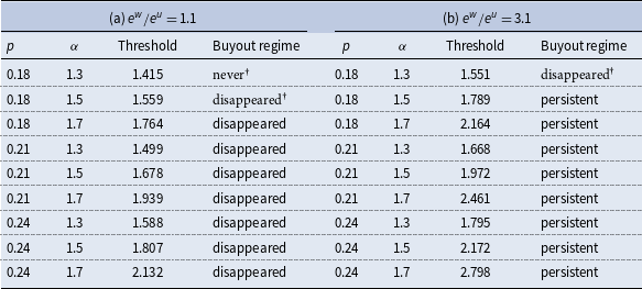
A table comparing buyout regimes under different conditions. The table has two panels, (a) and (b), each with different endowment ratios. Panel (a) has an endowment ratio of 1.1, and Panel (b) has an endowment ratio of 3.1. Each panel contains data for different values of rho (ρ) and alpha (α), along with corresponding threshold values and buyout regimes. The columns are labeled as follows: ρ, α, Threshold, and Buyout regime. Panel (a) data: Row 1: ρ 0.18, α 1.3, Threshold 1.415, Buyout regime never†. Row 2: ρ 0.18, α 1.5, Threshold 1.559, Buyout regime disappeared†. Row 3: ρ 0.18, α 1.7, Threshold 1.764, Buyout regime disappeared. Row 4: ρ 0.21, α 1.3, Threshold 1.499, Buyout regime disappeared. Row 5: ρ 0.21, α 1.5, Threshold 1.678, Buyout regime disappeared. Row 6: ρ 0.21, α 1.7, Threshold 1.939, Buyout regime disappeared. Row 7: ρ 0.24, α 1.3, Threshold 1.588, Buyout regime disappeared. Row 8: ρ 0.24, α 1.5, Threshold 1.807, Buyout regime disappeared. Row 9: ρ 0.24, α 1.7, Threshold 2.132, Buyout regime disappeared. Panel (b) data: Row 1: ρ 0.18, α 1.3, Threshold 1.551, Buyout regime disappeared†. Row 2: ρ 0.18, α 1.5, Threshold 1.789, Buyout regime persistent. Row 3: ρ 0.18, α 1.7, Threshold 2.164, Buyout regime persistent. Row 4: ρ 0.21, α 1.3, Threshold 1.668, Buyout regime persistent. Row 5: ρ 0.21, α 1.5, Threshold 1.972, Buyout regime persistent. Row 6: ρ 0.21, α 1.7, Threshold 2.461, Buyout regime persistent. Row 7: ρ 0.24, α 1.3, Threshold 1.795, Buyout regime persistent. Row 8: ρ 0.24, α 1.5, Threshold 2.172, Buyout regime persistent. Row 9: ρ 0.24, α 1.7, Threshold 2.798, Buyout regime persistent. The table notes that each subtable reports results for a fixed endowment ratio. The buyout regime is classified as never, disappeared, or persistent based on simulations. Cases marked with † fall into an innovation-stagnation state and are outside the domain where the asymptotic threshold is behaviorally relevant.
Notes: Each subtable reports results for a fixed endowment ratio (left: 1.1, right: 3.1). The column “Threshold” reports the theoretical inequality threshold implied by Proposition 1 for the corresponding pair
 $(p,\alpha )$
. The buyout regime is classified from the 800-period simulations as “never” (no buyouts in any period), “disappeared” (buyouts appear transiently and vanish in the long run), or “persistent” (buyouts remain active asymptotically). †For the parameter configurations marked with †, the economy falls into an innovation-stagnation state; these cases satisfy Lemma 3 and are therefore outside the domain where the asymptotic threshold is behaviorally relevant.
6.4 Sensitivity analysis
Building on the benchmark examples above, we next explore how the model’s buyout regimes respond to changes in the key parameters that enter the inequality threshold in Proposition 1. In particular, we vary the maximum success probability
 $p$
, the intensity of non-pecuniary entrepreneurial utility
 $\alpha$
, and the endowment ratio
 $e^w/e^u$
, and examine how the simulated regime classification lines up with the theoretical threshold.
Table 4 summarizes the results. For each configuration, we compute the implied inequality threshold from Proposition 1, compare it to the chosen endowment ratio, and classify the simulated economy as exhibiting no buyouts, disappearing buyouts, or persistent buyouts.
The sensitivity results are consistent with the mechanism highlighted in Proposition 1 and with the benchmark examples in the previous subsection. For each value of the success probability
 $p$
, increasing the non-pecuniary taste parameter
 $\alpha$
raises the required inequality threshold because under-endowed agents must be compensated more for giving up entrepreneurial control, and higher
 $p$
similarly raises the threshold by increasing the value of future entrepreneurial payoffs. In the simulations, whenever the economy remains in the sustained innovation region where Proposition 1 applies, buyout activity is persistent precisely when the observed endowment ratio exceeds the theoretical threshold. For example, with
 $p=0.18$
and
 $\alpha =1.5$
, the implied threshold is
 $1.789$
; when inequality is low (
 $e^w/e^u=1.1\lt 1.789$
) buyouts eventually disappear, whereas with high-inequality (
 $e^w/e^u=3.1\gt 1.789$
) buyout activity persists. The same pattern holds across the higher values of
 $p$
: for
 $p=0.21$
and
 $p=0.24$
, economies with
 $e^w/e^u=3.1$
always exhibit persistent buyouts once the threshold is exceeded, while economies with
 $e^w/e^u=1.1$
lie below the threshold and display only transient buyouts that eventually vanish.
The three parameter configurations marked with a dagger in Table 4 are noteworthy. When both the success probability
 $p$
and the entrepreneurial taste
 $\alpha$
are low, either well-endowed agents’ incomes remain too small, or the attractiveness of entrepreneurship is too limited for the economy to escape the low-innovation region characterized by Lemma 3. In these cases, the simulated path converges to an innovation-stagnation state with no sustained entrepreneurial activity, so the asymptotic threshold from Proposition 1 ceases to be a meaningful predictor of buyout persistence even when the observed endowment ratio exceeds the formal threshold.
Overall, the sensitivity analysis confirms that our main comparative-static insight is robust and complements the numerical examples above. Higher success probabilities and stronger non-pecuniary motives for entrepreneurship both increase the compensation that under-endowed agents require to sell their ideas, thereby raising the inequality threshold needed to sustain buyouts. When this threshold is met, and the economy escapes the stagnation region, buyout activity persists and continues to contribute to long-run variety growth, whereas economies with more equal endowments or weaker entrepreneurial prospects exhibit at most transient buyout episodes before reverting to a no-buyout regime.
7. Conclusion
This paper develops a novel theoretical framework that endogenizes the emergence of buyout funds through income-dependent risk preferences in an expanding variety growth model. Our analysis yields three key insights about the relationship between inequality, financial intermediation, and growth:
First, the model demonstrates that buyout funds arise endogenously as optimal contracts when initial endowment disparities exceed a critical threshold. The mechanism operates through two complementary channels: well-endowed agents’ willingness to sacrifice consumption for the non-pecuniary benefits of entrepreneurial participation, and under-endowed agents’ optimal decision to sell ideas when acquisition prices compensate for relinquished entrepreneurial utility.
Second, the persistence of buyouts depends fundamentally on the degree of inequality. In economies with large initial disparities, buyouts become permanent institutions because the required compensation grows proportionally with under-endowed agents’ incomes. Conversely, moderate inequality leads to transitional buyout phases that fade as growth enables independent entrepreneurship—a dynamic consistent with observed patterns of entrepreneurial spawning.
Third, the growth effects of buyouts vary systematically with inequality levels. While always providing an initial growth impulse through improved project allocation, buyouts generate sustained growth acceleration only in high-inequality regimes. In more equal economies, their role as transitional institutions gives way to decentralized innovation as wages rise.
These results offer a unified explanation for several empirical regularities in private equity markets while providing new theoretical insights about inequality’s dual role as both a catalyst and a constraint in innovation-driven growth. The framework suggests that optimal financial architecture evolves endogenously with development, with buyout funds serving distinct functions at different stages of economic maturation.
Acknowledgments
We are grateful to Akiomi Kitagawa, Koji Asano, and Jun Nagayasu for helpful discussions and valuable comments. We also thank three anonymous referees for their constructive suggestions, which substantially improved the paper.
Appendix A. Proofs and derivations
Proof of Lemma 1. Under self-sufficiency, an under-endowed agent with a business idea chooses savings
 $s_t^u$
and entrepreneurial investment
 $I_t^u$
to maximize
 \begin{equation*} \ln c^{u}_{t} + \beta \left [ \ln \left ( r_{t+1} (s^u_t - I^u_t) \right ) + p_t^u \left(R^E_{t+1} \right)^\alpha \right ], \quad \alpha \gt 1, \end{equation*}
subject to
 $c_t^u = w_t e^u - s_t^u$
and
 $0 \le I_t^u \le s_t^u \lt w_t e^u$
. The success probability is
 $p_t^u = \max \{0,p - 1/I_t^u\}$
.
(i) Case
 $p_t^u = 0$
.
When
 $p_t^u = 0$
, the agent has no effective entrepreneurial opportunity and sets
 $I_t^u = 0$
. The problem reduces to the standard consumption-saving decision:
 \begin{equation*} \max _{0\lt s_t^u\lt w_t e^u} {\ln} (w_t e^u - s_t^u) + \beta \ln \bigl (r_{t+1} s_t^u\bigr ). \end{equation*}
The FOC with respect to
 $s_t^u$
is
 \begin{equation*} -\frac {1}{w_t e^u - s_t^u} + \beta \frac {1}{s_t^u} = 0, \end{equation*}
which implies
 \begin{equation*} s_t^u = \frac {\beta }{1+\beta } w_t e^u. \end{equation*}
Therefore,
 \begin{equation*} (s_t^u, I_t^u) = \left (\frac {\beta w_t e^u}{1+\beta }, 0\right ) \end{equation*}
as stated in the lemma. Substituting back into the utility yields the indirect utility
 \begin{equation} (1+\beta )\ln (w_t e^u) + \beta \ln r_{t+1} - \ln \frac {(1+\beta )^{1+\beta }}{\beta ^\beta }, \end{equation}
which corresponds to the reservation utility in the main text.
(ii) Case
 $p_t^u = p - 1/I_t^u \gt 0$
and
 $p w_t e^u \le 1$
.
When
 $p_t^u\gt 0$
, the agent chooses
 $I_t^u\gt 0$
and
 $s_t^u \gt I_t^u$
. Conditional on a given
 $I_t^u$
, the problem in
 $s_t^u$
is identical to the previous case except that current resources are
 $w_t e^u - I_t^u$
. Thus, the FOC implies
 \begin{equation*} s_t^u = \frac {\beta }{1+\beta }(w_t e^u - I_t^u) + I_t^u = \frac {I_t^u + \beta w_t e^u}{1+\beta }. \end{equation*}
Hence any candidate optimum with positive entrepreneurship must have
 \begin{equation} (s_t^u, I_t^u) = \left (\frac {(I_t^u)^* + \beta w_t e^u}{1+\beta }, (I_t^u)^*\right ), \end{equation}
where
 $(I_t^u)^*\gt 0$
is chosen optimally. The success probability constraint
 $p_t^u = p - 1/I_t^u \gt 0$
requires
 \begin{equation*} (I_t^u)^* \gt \frac {1}{p}. \end{equation*}
If
 $p w_t e^u \le 1$
, the feasible set for
 $I_t^u$
is contained in
 $(0,w_t e^u)$
, which cannot accommodate
 $(I_t^u)^* \gt 1/p$
. Hence, in this case no entrepreneurial investment is feasible and the agent must choose
 $I_t^u=0$
, proving part (a) of the lemma.
(iii) Case
 $p w_t e^u \gt 1$
.
Now consider
 $p w_t e^u \gt 1$
, so that
 $I_t^u\gt 1/p$
is feasible. We compare the indirect utility from entrepreneurship with the non-entrepreneurial indirect utility. The key difference is summarized in equation (15) in the main text. Using the optimal
 $s_t^u$
derived above, the condition for entrepreneurship to be (weakly) preferred reduces to the sign of
 \begin{equation*} \ln \left (1 - \frac {(I_t^u)^*}{w_t e^u}\right ) + \frac {\beta }{1+\beta }\left [p - \frac {1}{(I_t^u)^*}\right ]\left(R^E_{t+1} \right)^\alpha . \end{equation*}
Define
 \begin{equation*} x \equiv 1 - \frac {(I_t^u)^*}{w_t e^u} \in \Bigl (0, 1 - \frac {1}{p w_t e^u}\Bigr ), \end{equation*}
so that
 $(I_t^u)^* = w_t e^u (1-x)$
, and note that
 $x$
is strictly between
 $0$
and
 $1$
when
 $pw_t e^u\gt 1$
. Substituting this into the expression above and using
 $p_t^u = p - 1/(I_t^u)^*, -(1+\beta )/[w_t e^u - (I_t^u)^*] + \beta \cdot (R_{t+1}^E)^\alpha /[(I_t^u)^*]^2= 0$
, we can rewrite the relevant term as
 \begin{equation*} f(x) \equiv \ln x + \frac {(1-x)\bigl [p w_t e^u (1-x) - 1\bigr ]}{x}. \end{equation*}
Thus, entrepreneurial investment is preferred if and only if
 $f(x) \ge 0$
.
We now establish the main properties of
 $f(x)$
:
-
• As
$x \downarrow 0$
, the term
$\ln x \to -\infty$
, while
$(1-x)\bigl [p w_t e^u (1-x) - 1\bigr ]/x \to +\infty$
dominates. A direct limit computation shows that
$f(x) \to +\infty$
as
$x \downarrow 0$
. -
• At the upper endpoint
$x = 1 - 1/(p w_t e^u)$
, we have
$p w_t e^u (1-x) - 1 = 0$
, so the second term vanishes and
\begin{equation*} f\bigl (1 - 1/(p w_t e^u)\bigr ) = \ln \bigl (1 - 1/(p w_t e^u)\bigr ) \lt 0. \end{equation*}
-
• A straightforward differentiation yields
which can be simplified to show that
\begin{equation*} f'(x) = \frac {1}{x} - \frac {(1-x)\bigl [p w_t e^u (1-x) - 1\bigr ]}{x^2} - \frac {\bigl [p w_t e^u (1-x) - 1\bigr ] - p w_t e^u (1-x)}{x} \end{equation*}
$f'(x)$
changes sign exactly once on the interval
$\bigl (0,1-1/(p w_t e^u)\bigr )$
.



These properties imply that there exists a unique solution
 $x(w_t)$
to
 $f(x)=0$
in the interval
 $\bigl (0,1-1/(p w_t e^u)\bigr )$
.
Equation (15) in the main text defines the threshold interest rate
 $r^u(w_t)$
by the condition that the under-endowed agent is indifferent between investing and not investing. Using the relationship between
 $x$
and
 $(I_t^u)^*$
, this indifference condition can be expressed in terms of
 $x(w_t)$
, so that
 $x(w_t)$
corresponds to the critical value of
 $1 - (I_t^u)^*/(w_t e^u)$
at
 $r_{t+1} = r^u(w_t)$
.
Next, note that
 $1 - (I_t^u)^*/w_t$
is a monotonically increasing function of
 $r_{t+1}$
, as follows from the expressions for monopoly profits and optimal investment, equations (8) and (14) in the main text. Combining this monotonicity with the uniqueness of
 $x(w_t)$
implies that
 $x(w_t) \gt x$
when
 $r_{t+1} \lt r^u(w_t)$
, and conversely when
 $r_{t+1} \gt r^u(w_t)$
. This completes the proof of the threshold characterization in equation (13).
(iv) Monotonicity and boundary condition for
 $r^u(w_t)$
.
Finally, we show that
 $r^u(w_t)$
is an increasing function of
 $w_t$
with
 $r^u(1/(p e^u))=0$
. By the definition of
 $x(w_t)$
, equation (15) can be rearranged as
 \begin{equation*} \left(R^E_{t+1} \right)^\alpha = \frac {(1+\beta )e^u}{\beta }\,\frac {w_t \bigl (1-x(w_t)\bigr )^2}{x(w_t)}. \end{equation*}
Since the left-hand side is decreasing in
 $r_{t+1}$
, it is sufficient to show that the right-hand side is decreasing in
 $w_t$
; then a larger
 $w_t$
requires a smaller
 $\left(R^E_{t+1} \right)^\alpha$
and hence a lower
 $r_{t+1}$
at indifference, implying that
 $r^u(w_t)$
is increasing in
 $w_t$
.
Define
 \begin{equation*} g(w) \equiv \frac {w\bigl (1-x(w)\bigr )^2}{x(w)}. \end{equation*}
We want to show
 $g'(w) \lt 0$
. Logarithmic differentiation of
 $g(w)$
yields
 \begin{equation} \frac {g'(w)}{g(w)} = \frac {1}{w} - \frac {x(w)+1}{x(w)\bigl (1-x(w)\bigr )}\,x'(w). \end{equation}
The function
 $x(w)$
is implicitly defined by
 $f(x(w))=0$
, which can be written as
 \begin{equation} \ln x(w) + \frac {\bigl (1-x(w)\bigr )\bigl [p w e^u (1-x(w))-1\bigr ]}{x(w)} = 0. \end{equation}
Differentiating eqaution (A4) with respect to
 $w$
and solving for
 $x'(w)$
gives
 \begin{equation} x'(w) = \frac {-(1-x)^2 p e^u}{\ln x + x(1-x)}. \end{equation}
In addition, rearranging eqaution (A4) for
 $w$
yields the relationship
 \begin{equation} w = \frac {1}{p e^u (1-x)^2}\,\bigl [(1-x) - x\ln x\bigr ]. \end{equation}
Substituting eqautions (A5) and (A6) into (A3) leads to
 \begin{equation} \frac {g'(w)}{g(w)} = \frac {p e^u (1-x)\bigl [-2x^2\ln x + x^2(1-x)^2 + 1 - x^2\bigr ]} {x(1-x-x\ln x)\bigl [\ln x + x(1-x)\bigr ]}. \end{equation}
For
 $x \in (0,1)$
we verify three inequalities:
 \begin{align*} \text{(a)}\quad & -2x^2\ln x + x^2(1-x)^2 + 1 - x^2 \gt 0, \\[3pt] \text{(b)}\quad & 1 - x - x\ln x \gt 0, \\[3pt] \text{(c)}\quad & \ln x + x(1-x) \lt x - 1 + x(1-x) = -(1-x)^2 \lt 0. \end{align*}
Given
 $p e^u\gt 0$
and
 $x(1-x)\gt 0$
, these inequalities imply that the numerator of
 $g'(w)/g(w)$
is positive, while the denominator is negative, so
 $g'(w) \lt 0$
. Hence
 $g(w)$
is decreasing in
 $w$
, and therefore
 $r^u(w_t)$
is an increasing function of
 $w_t$
.
To verify the boundary condition
 $r^u(1/(p e^u)) = 0$
, rewrite eqaution (A6) as
 \begin{equation*} p w_t e^u - 1 = \frac {x(w_t)\bigl (1 - x(w_t) - \ln x(w_t)\bigr )}{\bigl (1-x(w_t)\bigr )^2}. \end{equation*}
As
 $w_t \downarrow 1/(p e^u)$
, the left-hand side converges to zero, which forces the right-hand side to converge to zero as well. Since
 $x(w_t)\in \bigl (0,1-1/(p w_t e^u)\bigr )$
, the only feasible limit is
 $x(w_t)\to 0$
. From the original threshold condition (15), this requires
 $r_{t+1} \to 0$
, so
 $r^u(1/(p e^u)) = 0$
. This completes the proof.
Proof of Lemma 2. We solve the Nash bargaining problem under
 $\theta \lt 1/2$
, in which competition among unmatched under-endowed agents implies that the under-endowed agent receives exactly her reservation utility
 $u^{ur}_t$
(i.e., the participation constraint binds). Using the variable transformation introduced in the text,
 \begin{equation*} \tilde s_t^w \equiv s_t^w+I_t^u,\quad \tilde s_t^u \equiv s_t^u-I_t^u,\quad \tilde I_t^w \equiv I_t^w+I_t^u,\quad a_t\equiv -I_t^u, \end{equation*}
the binding participation constraint can be written as
 \begin{equation} \ln \!\big (w_t e^u+a_t-\tilde s_t^u\big )+\beta \ln \!\big (r_{t+1}\tilde s_t^u\big )=u^{ur}_t. \end{equation}
Given any transfer
 $a_t$
, the under-endowed agent chooses
 $\tilde s_t^u$
to satisfy eqaution (A8). The standard consumption-saving FOC implies
 \begin{equation} \tilde s_t^u=\frac {\beta }{1+\beta }(w_t e^u+a_t), \end{equation}
and substituting eqaution (A9) into (A8) yields the implied indirect utility on the left-hand side:
 \begin{equation} \ln (w_t e^u+a_t)+\beta \ln r_{t+1}-\ln \frac {(1+\beta )^{1+\beta }}{\beta ^\beta }. \end{equation}
Because the participation constraint binds, Eqaution (A10) must equal the reservation utility
 $u_t^{ur}$
derived in Lemma 1. We therefore determine
 $a_t$
by equating eqaution (A10) to the relevant expression for
 $u_t^{ur}$
.
Case (a): no entrepreneurship in autarky. When
 $w_t \le 1/(pe^u)$
, or when
 $w_t\gt 1/(pe^u)$
but
 $r^u(w_t)\le r_{t+1}$
, Lemma 1 implies that the under-endowed agent does not invest and her reservation utility is
 \begin{equation*} u^{ur}_t=(1+\beta )\ln (w_t e^u)+\beta \ln r_{t+1}-\ln \frac {(1+\beta )^{1+\beta }}{\beta ^\beta }. \end{equation*}
Equating this to eqaution (A10) gives
 $\ln (w_t e^u+a_t)=\ln (w_t e^u)$
, hence
 $a_t=0$
, establishing eqaution (24).
Case (b): entrepreneurship in autarky. When
 $w_t\gt 1/(pe^u)$
and
 $0\le r_{t+1}\le r^u(w_t)$
, Lemma 1 implies that the under-endowed agent chooses
 $(I_t^u)^*\gt 0$
and her reservation utility is
 \begin{equation*} u^{ur}_t=(1+\beta )\ln \!\big (w_t e^u-(I_t^u)^*\big ) +\beta \Big (p-\frac {1}{(I_t^u)^*}\Big )\left(R^E_{t+1} \right)^\alpha +\beta \ln r_{t+1} -\ln \frac {(1+\beta )^{1+\beta }}{\beta ^\beta }. \end{equation*}
Equating this expression to eqaution (A10) and canceling common terms yields
 \begin{equation*} \ln (w_t e^u+a_t) = \ln \!\big (w_t e^u-(I_t^u)^*\big ) +\frac {\beta }{1+\beta }\Big (p-\frac {1}{(I_t^u)^*}\Big )\left(R^E_{t+1} \right)^\alpha . \end{equation*}
Exponentiating both sides and solving for
 $a_t$
gives
 \begin{equation*} w_t e^u+a_t = \big [w_t e^u-(I_t^u)^*\big ] \exp \!\left \{\frac {\beta }{1+\beta }\Big [p-\frac {1}{(I_t^u)^*}\Big ]\left(R^E_{t+1} \right)^\alpha \right \}, \end{equation*}
which is equivalent to eqaution (25). This completes the proof.
Derivation of limit conditions in Section 4.2
We now provide the derivation of the limit conditions used in Section 4.2 for the case of sustained innovation without buyouts.
As the number of varieties
 $N_t$
grows without bound, the growth rate of varieties approaches unity. From the law of motion for varieties in the under-endowed–only regime,
 \begin{equation*} N_t - N_{t-1} = (1-\theta )\bigl [p - 1/(I^u_{t-1})^*\bigr ] L, \end{equation*}
we obtain
 \begin{equation} \lim _{t\to \infty }\frac {N_{t-1}}{N_t} = \lim _{t\to \infty }\left [1 - \frac {N_t - N_{t-1}}{N_t}\right ] = 1, \end{equation}
since
 $N_t \to \infty$
while the numerator in
 $(N_t - N_{t-1})/N_t$
remains bounded.
The factor price frontier in the main text (equation (9)) can be rewritten as
 \begin{equation*} \left (\frac {w_t}{N_t}\right )^\zeta r_t^{1-\zeta } = \left (\frac {\zeta }{1-\zeta }\right )^\zeta \left [1 + \biggl (\frac {N_t}{N_{t-1}} - 1\biggr )(1-\zeta )\right ]^\zeta . \end{equation*}
Using equation (A11), the right-hand side converges to
 $(\zeta /(1-\zeta ))^\zeta$
, so we obtain
 \begin{equation} \lim _{t\to \infty }\left (\frac {w_t}{N_t}\right )^\zeta r_t^{1-\zeta } = \left (\frac {\zeta }{1-\zeta }\right )^\zeta . \end{equation}
Next, capital market clearing imposes a relationship between
 $w_t/N_t$
and
 $r_{t+1}$
. Using the optimal savings decisions
 $s^i_t - I^i_t = \frac {\beta }{1+\beta }(w_t e^i - I^i_t)$
and the fact that the total investment share vanishes asymptotically (see below), the capital market equilibrium simplifies in the limit to
 \begin{equation} \lim _{t\to \infty }\left (\frac {w_t}{N_t}\right )^\zeta r_{t+1} = \left (\frac {1+\beta }{\beta }\right )^\zeta . \end{equation}
Combining equations (A12) and (A13) implies that the interest rate remains bounded:
 \begin{equation} 0 \lt \liminf _{t\to \infty }r_t \leq \limsup _{t\to \infty }r_t \lt \infty . \end{equation}
Given equation (A12) and the boundedness of
 $r_t$
, we must have
 \begin{equation} \lim _{t\to \infty }w_t = \infty , \qquad \lim _{t\to \infty }(I^u_t)^* = \infty , \end{equation}
because each new variety requires a fixed amount of capital and labor, and the wage bill grows with
 $N_t$
. However, the optimal investment-to-income ratio converges to zero:
 \begin{equation} \lim _{t\to \infty }\frac {(I^u_t)^*}{w_t} = 0. \end{equation}
This follows from the FOC for
 $(I^u_t)^*$
, which implies that the marginal benefit of entrepreneurial investment must equal its marginal cost; as
 $w_t$
grows, the marginal cost in terms of foregone consumption rises, forcing the share
 $(I^u_t)^*/w_t$
to shrink even though
 $(I^u_t)^*$
itself diverges.
Solving equations (A12) and (A13) jointly for the limits of
 $r_t$
and
 $w_t/N_t$
yields
 \begin{equation} \lim _{t\to \infty }r_t = \frac {1+\beta }{\beta }\cdot \frac {1-\zeta }{\zeta }, \end{equation}
and
 \begin{equation} \lim _{t\to \infty }\frac {w_t}{N_t} = \left (\frac {\beta }{1+\beta }\right )^{(1-\zeta )/\zeta } \left (\frac {\zeta }{1-\zeta }\right )^{1/\zeta }, \end{equation}
as reported in Section 4.2.
Finally, we note that entrepreneurial participation remains optimal along this growth path because the net benefit of innovation converges to a strictly positive constant:
 \begin{equation*} \frac {\beta }{1+\beta }p(R^E)^\alpha \gt 0, \end{equation*}
which is the limit of the left-hand side of equation (15. This ensures that innovation by under-endowed entrepreneurs is sustained asymptotically.
Proof of Lemma 3. Lemma 3 Characterizes the no-innovation steady state in which under-endowed agents never find entrepreneurship optimal. The key step is to identify when the under-endowed agent is exactly indifferent between investing and not investing in the steady state.
In the no-innovation steady state,
 $N_t$
is constant and the interest rate converges to a constant
 $\overline {r}$
. The comparison between the indirect utilities in equations (16) and (17) shows that entrepreneurial attempts depend on the sign of the left-hand side of equation (15): positive values induce entrepreneurship, negative values discourage it, and zero makes agents indifferent.
As
 $t\to +\infty$
, the interest rate converges to
 $\overline {r}$
, leading monopoly profits to approach
 \begin{equation} \lim _{t\to +\infty }R^E_{t+1}=\zeta \left (\frac {1-\zeta }{\overline {r}}\right )^{(1-\zeta )/\zeta }L\overline {e}\equiv R^E. \end{equation}
Substituting this limit into the indifference condition (15), we obtain
 \begin{equation} \ln \left [1-\frac {(I^u)^*}{\overline {w} e^u}\right ]+\frac {\beta }{1+\beta }\left [p-\frac {1}{(I^u)^*}\right ](R^E)^\alpha = 0, \end{equation}
where
 $(I^u)^* \gt 0$
is the steady-state entrepreneurial investment chosen under self-sufficiency and
 $\overline {w}$
is the steady-state wage.
To express
 $(I^u)^*$
in terms of the no-innovation variety level
 $\overline {N}$
, note that
 $\overline {w} = A\overline {N}$
in this steady state (see the main text), where
 $A$
is a positive constant. The optimality conditions for entrepreneurial investment imply the ratios
 \begin{equation} \frac {(I^u)^*}{\overline {w}e^u}\equiv \frac {2}{1+\sqrt {1+\frac {4A e^u (1+\beta )\overline {N}}{\beta (R^E)^\alpha }}}, \end{equation}
and
 \begin{equation} \frac {1}{(I^u)^*}\equiv \frac {\frac {1}{A\overline {N}}+\sqrt {\frac {1}{(A\overline {N})^2}+\frac {4e^u (1+\beta )}{\beta (R^E)^\alpha A\overline {N}}}}{2 e^u}. \end{equation}
These expressions show that both
 $\frac {(I^u)^*}{\overline {w}e^u}$
and
 $\frac {1}{(I^u)^*}$
are smooth functions of
 $\overline {N}$
. In particular:
-
• As
$\overline {N}\to 0$
, we have
$(I^u)^*/(\overline {w}e^u)\to 1$
and
$1/(I^u)^*\to +\infty$
. -
• As
$\overline {N}\to \infty$
, we have
$(I^u)^*/(\overline {w}e^u)\to 0$
and
$1/(I^u)^*\to 0$
. -
• Both
$(I^u)^*/(\overline {w}e^u)$
and
$1/(I^u)^*$
are monotone functions of
$\overline {N}$
.


Substituting equations (A21) and (A22) into (A20), we can write the left-hand side of equation (A20) as a function of
 $\overline {N}$
, say
 $f(\overline {N})$
. By continuity and the monotonicity properties above,
 $f(\overline {N})$
has the following characteristics:
-
• As
$\overline {N}\to 0$
, the term
$\ln \bigl [1-(I^u)^*/(\overline {w} e^u)\bigr ]$
dominates and
$f(\overline {N})\to -\infty$
. -
• As
$\overline {N}\to \infty$
,
$(I^u)^*/(\overline {w}e^u)\to 0$
and
$1/(I^u)^*\to 0$
, so
\begin{equation*} f(\overline {N}) \to \frac {\beta }{1+\beta }p(R^E)^\alpha \gt 0. \end{equation*}
-
• Direct differentiation (omitted for brevity) shows that
$f(\overline {N})$
is strictly increasing in
$\overline {N}$
.


These properties guarantee the existence of a unique threshold
 $\overline {N}^*$
such that
 $f(\overline {N}^*)=0$
, with
 $f(\overline {N})\lt 0$
for
 $\overline {N}\lt ne{N}^*$
and
 $f(\overline {N})\gt 0$
for
 $\overline {N}\gt \overline {N}^*$
.
Therefore, in the no-innovation steady state, entrepreneurial investment is not attractive (i.e., under-endowed agents strictly prefer not to invest) precisely when
 $\overline {N}\le \overline {N}^*$
. Using
 $\overline {w}=A\overline {N}$
, this condition is equivalent to
 $\overline {w}\le A\overline {N}^*$
, which is the wage bound stated in Lemma 3. This completes the proof.
Appendix B. Generalized nash bargaining analysis
B.1 Generalized nash bargaining
This appendix analyzes the robustness of the buyout persistence condition under generalized Nash bargaining, where under-endowed agents have bargaining power
 $\phi \in (0,1)$
and well-endowed agents have bargaining power
 $1-\phi$
. The generalized Nash product is
 \begin{equation} \left ( u^w_t - u^{wr}_t \right )^{1-\phi } \left ( u^u_t - u^{ur}_t \right )^{\phi }, \end{equation}
where
 $u^w_t$
and
 $u^u_t$
are the utilities of well-endowed and under-endowed agents in the match, respectively, and
 $u^{wr}_t$
and
 $u^{ur}_t$
are their reservation utilities from self-sufficiency. The bargaining problem chooses the transfer
 $a_t$
and the entrepreneurial investment
 $\tilde {I}_t^w$
to maximize this product, subject to the same constraints as in the baseline model.
B.1.1 Optimal investment decision
The FOC with respect to
 $\tilde {I}_t^w$
is
 \begin{equation} \frac {\partial u^w_t}{\partial \tilde {I}_t^w} = \frac {1}{w_t e^w - a_t - \tilde {I}_t^w} - \frac {\beta }{1+\beta } \frac {(R_{t+1}^w)^\alpha }{(\tilde {I}_t^w)^2} = 0. \end{equation}
This yields the same optimal investment rule as in the baseline model:
 \begin{equation} \tilde {I}_t^w = \frac {2(w_t e^w - a_t)}{1 + \sqrt {1 + \frac {4(1+\beta )(w_t e^w - a_t)}{\beta (R_{t+1}^w)^\alpha }}}. \end{equation}
As
 $t \to \infty$
, with sustained innovation we have
 $w_t \to \infty$
. From equation (B25), it follows that
 \begin{equation} \lim _{t \to \infty } \frac {\tilde {I}_t^w}{w_t} = 0. \end{equation}
Thus, the entrepreneurial investment choice has the same asymptotic behavior regardless of the bargaining power distribution.
B.1.2 Optimal transfer and profit-sharing
The FOC with respect to
 $a_t$
is
 \begin{equation} \frac {1-\phi }{u^w_t - u^{wr}_t } \frac {\partial u^w_t}{\partial a_t} + \frac {\phi }{u^u_t - u^{ur}_t} \frac {\partial u^u_t}{\partial a_t} = 0, \end{equation}
where
 \begin{align} \frac {\partial u^w_t}{\partial a_t} &= -\frac {1}{w_t e^w - a_t - \tilde {I}_t^w}, \\[-10pt] \nonumber \end{align}
 \begin{align} \frac {\partial u^u_t}{\partial a_t} &= \frac {1}{w_t e^u + a_t}. \\[10pt] \nonumber \end{align}
In the baseline model (where under-endowed agents have no bargaining power), the profit share is at a corner,
 $R^w_{t+1} = R^E_{t+1}$
, when
 $\alpha \gt 1$
. With
 $\phi \gt 0$
, the profit share may instead be interior. The FOC with respect to
 $R^w_{t+1}$
for an interior solution is
 \begin{equation} \frac {1-\phi }{u^w_t - u^{wr}_t } \frac {\partial u^w_t}{\partial R^w_{t+1}} + \frac {\phi }{u^u_t - u^{ur}_t} \frac {\partial u^u_t}{\partial R^w_{t+1}} = 0, \end{equation}
where
 \begin{align} \frac {\partial u^w_t}{\partial R^w_{t+1}} &= \Bigl (p - \frac {1}{ \tilde {I}_t^w} \Bigr ) \cdot \alpha (R^w_{t+1})^{\alpha -1}, \\[-10pt] \nonumber \end{align}
 \begin{align} \frac {\partial u^u_t}{\partial R^w_{t+1}} &= -\Bigl (p - \frac {1}{ \tilde {I}_t^w} \Bigr ) \cdot \alpha (R^E_{t+1}-R^w_{t+1})^{\alpha -1}.\\[10pt] \nonumber \end{align}
The equilibrium with buyouts is characterized by the transfer
 $a_t$
and the profit share
 $\gamma _t \equiv R_{t+1}^w / R_{t+1}^E$
. In the long run, we define the limiting transfer ratio
 $\tau = \lim _{t\to \infty } a_t / w_t$
and the limiting profit share
 $\gamma = \lim _{t\to \infty } \gamma _t$
. Analogous to the analysis in Section 4.3, the utility differences converge to:
 \begin{align} u^w_t - u^{wr}_t &\to (1+\beta ) \ln \!\left (1 - \frac {\tau }{e^w}\right ) + \beta p (R^E)^\alpha \gamma ^\alpha , \\[-10pt] \nonumber \end{align}
 \begin{align} u^u_t - u^{ur}_t &\to (1+\beta ) \ln \!\left (1 + \frac {\tau }{e^u}\right ) + \beta p (R^E)^\alpha \bigl [(1-\gamma )^\alpha - 1\bigr ]. \\[10pt] \nonumber \end{align}
The limiting FOCs from the Nash bargaining problem then imply
 \begin{align} \frac {(1+\beta ) \ln \!\left (1 + \frac {\tau }{e^u}\right ) + \beta p (R^E)^\alpha \bigl [(1-\gamma )^\alpha - 1\bigr ]} {(1+\beta ) \ln \!\left (1 - \frac {\tau }{e^w}\right ) + \beta p (R^E)^\alpha \gamma ^\alpha } &= \frac {\phi }{1-\phi }\,\frac {e^w-\tau }{e^u + \tau }, \\[-10pt] \nonumber \end{align}
 \begin{align} \frac {(1+\beta ) \ln \!\left (1 + \frac {\tau }{e^u}\right ) + \beta p (R^E)^\alpha \bigl [(1-\gamma )^\alpha - 1\bigr ]} {(1+\beta ) \ln \!\left (1 - \frac {\tau }{e^w}\right ) + \beta p (R^E)^\alpha \gamma ^\alpha } &= \frac {\phi }{1-\phi }\, \frac {(1-\gamma )^{\alpha -1}}{\gamma ^{\alpha -1}}. \\[10pt] \nonumber \end{align}
Equations (B35) and (B36) jointly determine the equilibrium pair
 $(\tau ,\gamma )$
for a given bargaining weight
 $\phi \in (0,1)$
.
B.2 Buyout persistence conditions
For buyouts to persist in the long run, both agents must receive at least their reservation utilities:
 \begin{align} (1+\beta ) \ln \!\left (1 - \frac {\tau }{e^w}\right ) + \beta p (R^E)^\alpha \gamma ^\alpha &\geq 0, \\[-10pt] \nonumber \end{align}
 \begin{align} (1+\beta ) \ln \!\left (1 + \frac {\tau }{e^u}\right ) + \beta p (R^E)^\alpha \bigl [(1-\gamma )^\alpha - 1\bigr ] &\geq 0. \\[10pt] \nonumber \end{align}
Define
 \begin{equation*} \kappa \equiv \frac {\beta p (R^E)^\alpha }{1+\beta }. \end{equation*}
From equation (B37) and (B38), we obtain necessary bounds on
 $\tau$
:
 \begin{align} \tau &\leq e^w \left [ 1 - \exp \left ( - \kappa \gamma ^\alpha \right ) \right ], \\[-10pt] \nonumber \end{align}
 \begin{align} \tau &\geq e^u \left [ \exp \left ( \kappa \bigl [1-(1-\gamma )^\alpha \bigr ] \right ) - 1 \right ]. \\[10pt] \nonumber \end{align}
For a feasible transfer
 $\tau$
to exist, the upper bound must be at least as large as the lower bound:
 \begin{equation} e^u \left [ \exp \left ( \kappa \bigl [1-(1-\gamma )^\alpha \bigr ] \right ) - 1 \right ] \leq e^w \left [ 1 - \exp \left ( - \kappa \gamma ^\alpha \right ) \right ]. \end{equation}
This yields a necessary condition on the endowment ratio:
 \begin{equation} \frac {e^w}{e^u} \;\geq \; \frac { \exp \left ( \kappa \bigl [1-(1-\gamma )^\alpha \bigr ] \right ) - 1 } { 1 - \exp \left ( - \kappa \gamma ^\alpha \right ) } \;\equiv \; B(\gamma ). \end{equation}
The function
 $B(\gamma )$
in equation (B42) determines the necessary endowment ratio for buyout persistence, conditional on the limiting profit share
 $\gamma$
:
-
1. Corner solution (
$\gamma = 1$
). When
$\gamma = 1$
(e.g., when
$\phi = 0$
and
$\alpha \gt 1$
so that the profit share is at a corner), we obtainwhich coincides with the baseline condition in Proposition 1. In this case, the condition is also sufficient for buyouts to persist, and
\begin{equation*} B(1) = \exp (\kappa ) = \exp \!\left ( \frac {\beta p (R^E)^\alpha }{1+\beta } \right ), \end{equation*}
$\tau$
is pinned down by equation (B35). To see this, consider a continuous function
$F(\tau )$
defined on the non-empty set
\begin{align*} \Bigl \{\tau \,\big |\, (1+\beta )\ln (1 - \tau /e^w) + \beta p (R^E)^\alpha \gt 0, \; (1+\beta )\ln (1 + \tau /e^u) - \beta p (R^E)^\alpha \gt 0 \Bigr \}: \\[-29pt] \end{align*}
Standard arguments show that there exists a unique
\begin{align*} F(\tau )\equiv \frac {(1+\beta )\ln (1 + \tau /e^u) - \beta p (R^E)^\alpha } {(1+\beta )\ln (1 - \tau /e^w) + \beta p (R^E)^\alpha } - \frac {\phi }{1-\phi } \cdot \frac {e^w - \tau }{e^u + \tau }. \end{align*}
$\tau$
in this domain satisfying
$F(\tau )=0$
.
-
2. Interior profit sharing (
$\phi \gt 0$
). For
$\phi \gt 0$
, the limiting profit share
$\gamma$
may be interior and is jointly determined with
$\tau$
by equations (B35) and (B36). The function
$B(\gamma )$
need not be monotone in
$\gamma$
; its shape depends on
$\alpha$
,
$\beta$
,
$p$
, and
$R^E$
. In cases where
$B(\gamma ) \lt B(1)$
at the equilibrium
$\gamma$
, the required endowment ratio is lower than in the baseline model, so generalized bargaining relaxes the buyout condition. Conversely, when
$B(\gamma ) \gt B(1)$
, a higher endowment ratio is required. In all interior cases, a buyout equilibrium requires a pair
$(\gamma , \tau )$
that simultaneously satisfies the FOCs (B35)–(B36) and lies in the feasible set defined by the participation constraints (B37)–(B38).


Overall, the generalized bargaining framework shows that allowing under-endowed agents to have bargaining power affects both the transfer
 $\tau$
and the profit share
 $\gamma$
, and can either tighten or relax the inequality threshold for persistent buyouts. However, the qualitative mechanism from the baseline model is robust: buyouts persist only when endowment disparities are large enough to support mutually beneficial transfers and risk sharing.
Appendix C. Robustness to alternative success probability specifications
The baseline model employs the functional form
 $ p_t = \max \big[0, p - \frac {1}{I_t}\big]$
for tractability. To assess the robustness of our results, we consider a general success probability function
 $ p(I_t)$
satisfying the following economically intuitive properties:
-
1. Boundedness:
$ p(I_t) \in [0, \overline {p}]$
where
$ \overline {p} \leq 1$
denotes the maximum achievable success probability. -
2. Concavity:
$ p'(I_t) \gt 0$
and
$ p''(I_t) \lt 0$
for
$ I_t \gt 0$
, capturing diminishing returns to investment. -
3. Asymptotic Flatness:
$ \lim _{I_t \to \infty } I_t \cdot p'(I_t) = 0$
, ensuring that marginal returns vanish sufficiently fast for large investments.


These properties are satisfied by both our baseline specification and smoother alternatives such as
 $ p(I_t) = 1 - e^{-\chi I_t}$
or
 $ p(I_t) = \frac {\chi I_t}{1 + \chi I_t}$
.
The optimization problem for under-endowed agents becomes:
 \begin{equation} \max _{I_t^u} \; (1+\beta )\ln (w_t e^u - I_t^u) + \beta p(I_t^u)(R_{t+1}^E)^\alpha . \end{equation}
The FOC is:
 \begin{equation} -\frac {1+\beta }{w_t e^u - I_t^u} + \beta p'(I_t^u)(R_{t+1}^E)^\alpha = 0. \end{equation}
Let
 $ (I_t^{u})^*$
denote the solution to equation (C44). Defining the investment ratio
 $ y_t = (I_t^{u})^* / w_t$
, we analyze its asymptotic properties as
 $ w_t \to \infty$
.
Lemma 4. For any success probability function
 $ p(I_t)$
satisfying the properties above, the optimal investment
 $ (I_t^{u})^*$
has the following properties:
-
1.
$ (I_t^{u})^*$
is strictly increasing in
$ w_t$
for sufficiently large
$ w_t$
. -
2.
$ \lim _{t \to \infty } (I_t^{u})^* = \infty$
. -
3.
$ \lim _{t \to \infty } y_t = 0$
.


Proof. Rewrite equation (C44) using
 $ y_t$
:
 \begin{equation} \frac {1+\beta }{1 - y_t} = \beta p'\left ((I_t^{u})^*\right )(R_{t+1}^E)^\alpha w_t. \end{equation}
As
 $ w_t \to \infty$
, a bounded
 $ (I_t^{u})^*$
would imply
 $ y_t \to 1$
, which would violate equation (C45). Rearranging gives:
 \begin{equation} \frac {y_t}{1 - y_t} = \frac {\beta (R_{t+1}^E)^\alpha }{1+\beta } (I_t^{u})^* p'\left ((I_t^{u})^*\right ). \end{equation}
By the asymptotic flatness condition,
 $ \lim _{(I_t^{u})^* \to \infty } (I_t^{u})^* p'\big ((I_t^{u})^*\big ) = 0$
. Hence, the right-hand side of equation (C46) converges to 0, which implies
 $ y_t \to 0$
. Monotonicity of
 $ (I_t^{u})^*$
in
 $ w_t$
for sufficiently large
 $ w_t$
then follows from equation (C45).
C.1 Implications for buyout persistence
The bargaining problem with a general success probability function has the same structure as in the baseline model. The key asymptotic results carry through.
Proposition 1 (Extended). Under a general success probability function
 $ p(I_t)$
satisfying the properties above, the condition for persistent buyouts in an economy with sustained innovation is
 \begin{equation} \frac {e^w}{e^u} \gt \exp \left ( \frac {\beta }{1+\beta } \overline {p} (R^E)^\alpha \right ), \end{equation}
where
 $ \overline {p} = \lim _{I \to \infty } p(I)$
is the maximum success probability.
Proof. The transfer ratio satisfies:
 \begin{equation} \frac {a_t}{w_t e^u} = \left [1 - \frac {(I_t^{u})^*}{w_t e^u}\right ] \exp \left \{\frac {\beta }{1+\beta } p\left ((I_t^{u})^*\right )(R_{t+1}^E)^\alpha \right \} - 1. \end{equation}
As
 $ t \to \infty$
, the lemma implies
 $ y_t = (I_t^{u})^*/w_t \to 0$
and, by boundedness and monotonicity,
 $ p\left ((I_t^{u})^*\right ) \to \overline {p}$
. Thus,
 \begin{equation} \lim _{t \to \infty } \frac {a_t}{w_t e^u} = \exp \left \{\frac {\beta }{1+\beta } \overline {p} (R^E)^\alpha \right \} - 1. \end{equation}
The participation condition for well-endowed agents then yields the stated inequality.
This analysis demonstrates that our main existence result is robust to the specific functional form of the success probability. The threshold condition for persistent buyouts depends only on the maximal attainable success probability
 $ \overline {p}$
, not on the detailed shape of
 $ p(I_t)$
. In particular, smoother specifications such as the exponential and rational forms discussed above deliver the same asymptotic condition.
Appendix D. Diversification, convex preferences, and portfolio concentration
The baseline assumes that each well-endowed agent acquires (and implements) at most one idea, that is, takes a concentrated entrepreneurial position. This section shows when such concentration is privately optimal once we allow the investor to split a fixed total entrepreneurial scale
 $I\gt 0$
across multiple independent ideas, and clarifies how strong convexity in the entrepreneurial utility component must be to overturn the standard diversification motive.
A project of scale
 $J$
succeeds with probability
 $p(J)$
and yields payoff
 $R^E$
upon success and
 $0$
otherwise. Let
 $v(\! \cdot \!)$
denote utility from the entrepreneurial payoff (holding safe wealth/consumption fixed). We compare two allocations of the same total scale
 $I$
:
(i) Concentrated: invest all
 $I$
in one idea, so
 \begin{equation*} U^{\text{conc}}(I)=p(I)\,v(R^E)+(1-p(I))\,v(0). \end{equation*}
(ii) Equally diversified: split
 $I$
across
 $n\ge 2$
independent ideas of scale
 $I/n$
. Let
 $k\sim \mathrm{Binomial}\!\big (n,p(I/n)\big )$
be the number of successes; then
 $X^{\text{div}}=kR^E$
and
 \begin{equation*} U^{\text{div}}(I,n)=\sum _{k=0}^n \binom {n}{k} p(I/n)^k\big (1-p(I/n)\big )^{n-k} v(kR^E). \end{equation*}
D.1 Linear benchmark: Diversification dominates
If
 $v(X)=aX+b$
with
 $a\gt 0$
, only the mean payoff matters:
 \begin{equation*} U^{\text{conc}}(I)=a\,p(I)R^E+b,\qquad U^{\text{div}}(I,n)=a\,n\,p(I/n)R^E+b. \end{equation*}
Under our maintained assumptions that
 $p(\! \cdot \!)$
is increasing and concave with
 $p(0)=0$
, concavity implies
 $p(I)\le n\,p(I/n)$
(strictly if
 $p$
is strictly concave). Hence
 \begin{equation*} U^{\text{div}}(I,n)\ge U^{\text{conc}}(I), \end{equation*}
so a risk-neutral investor strictly prefers diversification. Therefore, concentrated buyout positions require a departure from linear entrepreneurial preferences.
D.2 Convex entrepreneurial utility: When concentration is optimal
In the main text,
 $v(\! \cdot \!)$
is strictly convex for entrepreneurial payoffs above the threshold,
 \begin{equation*} v''(X)\gt 0\quad \text{for } X\ge \bar X. \end{equation*}
Diversification raises the mean entrepreneurial payoff (because
 $p$
is concave) but reduces payoff dispersion (because it pools independent risks). With convex
 $v$
, lower dispersion is costly in utility terms, creating a force toward concentration.
To quantify how much convexity is needed, consider
 $v(X)=X^{1+\eta }$
with
 $\eta \gt 0$
. Then there exists a cutoff
 $\eta ^\ast (I,R^E,p,\bar X)\gt 0$
such that
 \begin{equation*} U^{\text{conc}}(I)\gt U^{\text{div}}(I,n)\quad \text{for all } n\ge 2 \quad \text{whenever } \eta \gt \eta ^\ast . \end{equation*}
Intuitively,
 $\eta ^\ast$
is higher when diversification generates a large mean gain (e.g., when success probabilities are high and/or marginal returns to scale in
 $p$
are strongly diminishing) and lower when entrepreneurial payoffs are more skewed (large
 $R^E$
relative to the threshold region), which increases the value of dispersion under convex preferences.
D.3 Baseline form: An explicit sufficient condition
Under the baseline success technology
 $p(I)=p-1/I$
(for
 $I\gt 1/p$
), a tractable sufficient condition for concentration is obtained by comparing the concentrated position to the
 $n=2$
split. With
 $v_\eta (X)=X^{1+\eta }$
and
 $v_\eta (0)=0$
, we have
 \begin{equation*} U^{\text{conc}}_\eta (I)=\Big (p-\frac {1}{I}\Big )(R^E)^{1+\eta }, \end{equation*}
and, for
 $n=2$
,
 \begin{equation*} U^{\text{div}}_\eta (I,2) =2q(1-q)(R^E)^{1+\eta }+q^2(2R^E)^{1+\eta }, \qquad q\equiv p\!\left (\frac {I}{2}\right )=p-\frac {2}{I}. \end{equation*}
Thus
 $U^{\text{conc}}_\eta (I)\gt U^{\text{div}}_\eta (I,2)$
holds whenever
 \begin{equation*} \Big (p-\frac {1}{I}\Big ) \;\gt \; 2q(1-q)+q^2\,2^{1+\eta }. \end{equation*}
Equivalently, a sufficient lower bound on the curvature parameter is
 \begin{equation*} \eta \;\gt \; \underline {\eta }(I) \;\equiv \; \log _2\!\left (\frac {p-\frac {1}{I}-2q(1-q)}{q^2}\right )-1, \qquad q=p-\frac {2}{I}, \end{equation*}
whenever the term inside
 $\log _2(\! \cdot \!)$
is greater than one. This bound is conservative but transparent: it quantifies how convex the entrepreneurial utility must be for a wealthy investor to prefer a single large buyout over even a minimal degree of diversification.
Overall, with linear entrepreneurial preferences investors would diversify, but with sufficiently convex
 $v(\! \cdot \!)$
a concentrated buyout position becomes privately optimal despite the availability of multiple independent ideas.






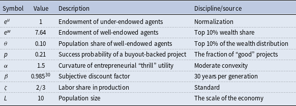
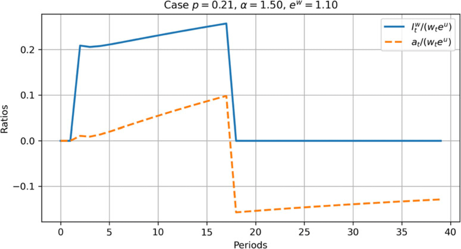
 Itw/(wteu)
 at/(wteu)

 ew/eu=1.1
 θ=0.1

 ew/eu=7.64
 θ=0.1