





1. Introduction
Submarine landslides flowing down a slope under gravity generally propagate with a high velocity and large translational momentum (Masson et al. Reference Masson, Harbitz, Wynn, Pedersen and Løvholt2006). They may result in catastrophic tsunamis (Grilli & Watts Reference Grilli and Watts2005; Liu et al. Reference Liu, Wu, Raichlen, Synolakis and Borrero2005; Sepúlveda & Serey Reference Sepúlveda and Serey2009; Ma et al. Reference Ma, Kirby, Hsu and Shi2015; Wang, Ward & Xiao Reference Wang, Ward and Xiao2015; George, Iverson & Cannon Reference George, Iverson and Cannon2017; Gylfadóttir et al. Reference Gylfadóttir, Kim, Helgason, Brynjólfsson, Höskuldsson, Jóhannesson, Harbitz and Løvholt2017; Clous & Abadie Reference Clous and Abadie2019; Grilli et al. Reference Grilli2021) and devastating deformation and fracture of offshore platforms and pipelines (López-Venegas et al. Reference López-Venegas, Horrillo, Pampell-Manis, Huérfano and Mercado2015). In the studies of landslide momentum and energy (Clous & Abadie Reference Clous and Abadie2019; Yavari-Ramshe & Ataie-Ashtiani Reference Yavari-Ramshe and Ataie-Ashtiani2019; Bregoli, Medina & Bateman Reference Bregoli, Medina and Bateman2021), it was shown that only a fairly small part of the landslide energy (6 % noted in Bregoli et al. Reference Bregoli, Medina and Bateman2021) was transferred to the generated tsunami while more than 50 % was dissipated by the basal friction in the further propagation. Hence, after the transfer of energy to waves, the remaining momentum of submarine landslides off a slope may still be high. The high remaining momentum can maintain a long extension of the landslides away from the slope and result in a great impact on submarine infrastructure. For instance, an impressive run-out up to 1500 km of submarine landslides together with generated turbidity currents has been reported (Talling et al. Reference Talling, Wynn, Masson, Frenz, Cronin, Schiebel, Akhmetzhanov, Dallmeier-Tiessen, Benetti and Weaver2007; Azpiroz-Zabala et al. Reference Azpiroz-Zabala, Cartigny, Talling, Parsons, Sumner, Clare, Simmons, Cooper and Pope2017). Therefore, other than the tsunami usually concerned, it is also critical to resolve the momentum variation of submarine landslides off the slope for the laying, protection and safety of submarine infrastructure.
However, only a very limited number of studies have focused on the momentum of deformable submarine landslides (Yavari-Ramshe & Ataie-Ashtiani Reference Yavari-Ramshe and Ataie-Ashtiani2019; Cabrera et al. Reference Cabrera, Pinzon, Take and Mulligan2020), not to mention the variation of momentum after the slides flow down the slope. Most of the existing studies on submarine landslides mainly pay attention to the properties of the generated tsunami (Watts et al. Reference Watts, Grilli, Kirby, Fryer and Tappin2003; Løvholt, Harbitz & Haugen Reference Løvholt, Harbitz and Haugen2005; Harbitz et al. Reference Harbitz, Løvholt, Pedersen and Masson2006; Yavari-Ramshe & Ataie-Ashtiani Reference Yavari-Ramshe and Ataie-Ashtiani2016; Takabatake et al. Reference Takabatake, Mäll, Han, Inagaki, Kisizaki, Esteban and Shibayama2020). A few investigated the characteristics of the deformable slide body but concentrated on the evolution of the slide shape (Shi et al. Reference Shi, An, Wu, Liu and Cao2016; Grilli et al. Reference Grilli, Shelby, Kimmoun, Dupont, Nicolsky, Ma, Kirby and Shi2017; Rauter Reference Rauter2021), the propagation velocity (Watts et al. Reference Watts, Grilli, Tappin and Fryer2005; Tajnesaie, Shakibaeinia & Hosseini Reference Tajnesaie, Shakibaeinia and Hosseini2018; Pilvar, Pouraghniaei & Shakibaeinia Reference Pilvar, Pouraghniaei and Shakibaeinia2019) or the run-out and the final deposit of the slides (Talling et al. Reference Talling, Wynn, Masson, Frenz, Cronin, Schiebel, Akhmetzhanov, Dallmeier-Tiessen, Benetti and Weaver2007; Elverhoi et al. Reference Elverhoi, Breien, De Blasio, Harbitz and Pagliardi2010; Parez & Aharonov Reference Parez and Aharonov2015). The few papers on the momentum or energy of deformable submarine landslides (Watts et al. Reference Watts, Grilli, Kirby, Fryer and Tappin2003; Ataie-Ashtiani & Najafi-Jilani Reference Ataie-Ashtiani and Najafi-Jilani2008; López-Venegas et al. Reference López-Venegas, Horrillo, Pampell-Manis, Huérfano and Mercado2015; Clous & Abadie Reference Clous and Abadie2019; Yavari-Ramshe & Ataie-Ashtiani Reference Yavari-Ramshe and Ataie-Ashtiani2019; Cabrera et al. Reference Cabrera, Pinzon, Take and Mulligan2020) were exclusively devoted to the estimation of the generated waves, focusing on the momentum/energy transfer in the wave generation stage. Until now, little attention has been paid to the variation of momentum of deformable submarine landslides when the slides flow away from the slope over a flat bottom.
In this paper, the translational momentum of deformable submarine landslides off a non-erodible slope is numerically investigated with a two-phase smoothed particle hydrodynamics (SPH) model (Shi, Yu & Dalrymple Reference Shi, Yu and Dalrymple2017; Shi et al. Reference Shi, Si, Dong and Yu2019, Reference Shi, Dong, Yu and Zhou2021). Yavari-Ramshe & Ataie-Ashtiani (Reference Yavari-Ramshe and Ataie-Ashtiani2016), Kirby et al. (Reference Kirby2022) and Lee et al. (Reference Lee, Lo, Shi and Huang2022) have provided comprehensive reviews of numerical models for submarine and subaerial landslides. Specifically, for deformable submarine landslides, four main types of numerical models have been developed. In the first type of landslide models, generally, the motion of the deformable landslide was prescribed and the deformation of the slide body was solved by empirical deformation models (Liu, Lynett & Synolakis Reference Liu, Lynett and Synolakis2003; Løvholt et al. Reference Løvholt, Pedersen, Harbitz, Glimsdal and Kim2015; Bregoli et al. Reference Bregoli, Medina and Bateman2021; Lo & Liu Reference Lo and Liu2021). In these models, the motion and the deformation of landslides were decoupled. To overcome this weakness, two-layer models, i.e. an upper layer of fluid for water and a lower layer of fluid for landslides, were developed to simulate the coupled movement and deformation of the landslides. The second main type of landslide models are depth-integrated two-layer ones, in which depth-integrated mass and momentum equations were utilized to describe the motion of both the slide and the water by assuming the slide to be a non-Newtonian fluid or granular flow (Heinrich Reference Heinrich1992; Jiang & LeBlond Reference Jiang and Leblond1992; Fernández-Nieto et al. Reference Fernández-Nieto, Bouchut, Bresch, Castro Diaz and Mangeney2008; Grilli et al. Reference Grilli, Shelby, Kimmoun, Dupont, Nicolsky, Ma, Kirby and Shi2017). The depth-integrated models could not resolve the variations of the velocities and other physical variables along the depth that were critical to the wave generation (Romano et al. Reference Romano, Lara, Barajas, Di Paolo, Bellotti, Di Risio, Losada and De Girolamo2020). Hence, the third main type of landslide models, i.e. the depth-resolved two-layer models, were proposed. In these models, the fully three-dimensional Navier–Stokes equations were adopted for both the slide and the water (Abadie et al. Reference Abadie, Morichon, Grilli and Glockner2010; Horrillo et al. Reference Horrillo, Wood, Kim and Parambath2013; Ma, Kirby & Shi Reference Ma, Kirby and Shi2013; Rauter et al. Reference Rauter, Hobe, Mulligan, Take and Løvholt2021). Combining the above two types of models, Ma et al. (Reference Ma, Kirby, Hsu and Shi2015) and Zhang et al. (Reference Zhang, Kirby, Shi, Ma and Grilli2021) developed hybrid models using depth-integrated equations for the slide layer and depth-resolved three-dimensional equations for the water layer. In the above three types of landslide models, the saturated underwater slide, which is a two-phase system composed of solid particles and interstitial water, was always taken as a whole Newtonian or non-Newtonian continuum. The velocity difference between the solid particles and the interstitial water was unsolved (Yavari-Ramshe & Ataie-Ashtiani Reference Yavari-Ramshe and Ataie-Ashtiani2016). However, in real landslide events, the two-phase nature of the slides could not be neglected (Yavari-Ramshe & Ataie-Ashtiani Reference Yavari-Ramshe and Ataie-Ashtiani2017; Lee et al. Reference Lee, Lo, Shi and Huang2022). Thus, the fourth main type of landslide models, i.e. multiphase models, have attracted lots of attention in the past decade. A few Eulerian–Eulerian models (phase-resolved Navier–Stokes equations for both the particle and the water phases in the slides, Meruane, Tamburrino & Roche Reference Meruane, Tamburrino and Roche2010; Armanini et al. Reference Armanini, Larcher, Nucci and Dumbser2014; Kaitna, Dietrich & Hsu Reference Kaitna, Dietrich and Hsu2014; Savage, Babaei & Dabros Reference Savage, Babaei and Dabros2014; Bouchut et al. Reference Bouchut, Fernández-Nieto, Mangeney and Narbona-Reina2016; Yavari-Ramshe & Ataie-Ashtiani Reference Yavari-Ramshe and Ataie-Ashtiani2017; Si, Shi & Yu Reference Si, Shi and Yu2018; Lee & Huang Reference Lee and Huang2021; Rauter Reference Rauter2021; Rauter et al. Reference Rauter, Viroulet, Gylfadóttir, Fellin and Løvholt2022) and Eulerian–Lagrangian models (phase-resolved Navier–Stokes equations for the water phase and Lagrangian particle tracking methods such as the discrete element method (DEM) for individual particles in the slides, Zhao, Utili & Crosta Reference Zhao, Utili and Crosta2016; Jiang, Shen & Wu Reference Jiang, Shen and Wu2018; Yang et al. Reference Yang, Jing, Kwok and Sobral2020; Nguyen Reference Nguyen2022) have been developed for deformable landslides. To capture the generated waves, meshless numerical methods such as SPH have been increasingly adopted to solve the governing equations (Ataie-Ashtiani & Shobeyri Reference Ataie-Ashtiani and Shobeyri2008; Tajnesaie et al. Reference Tajnesaie, Shakibaeinia and Hosseini2018; Shi et al. Reference Shi, Dong, Yu and Zhou2021; Lee et al. Reference Lee, Lo, Shi and Huang2022). In the present study, the momentum of both the particle and the water phases in deformable submarine landslides is investigated and hence a two-phase model is preferred.
Rather than focusing on the momentum transfer from the slide to the tsunami (Mulligan & Take Reference Mulligan and Take2017), this study concentrates on the variation of the slide translational momentum along the propagation over a flat bottom after the slide flows down the slope. It is helpful for engineering design purposes in estimating the potential impact on submarine infrastructure (López-Venegas et al. Reference López-Venegas, Horrillo, Pampell-Manis, Huérfano and Mercado2015). The transport rate and flux of the slide translational momentum along the propagation path off the slope are examined. The effect of sediment suspension from the slide body on the variation of the translational momentum is illustrated. Moreover, the effects of landslide physical properties, specifically the grain size, the initial compaction and the initial front intrusion angle, are intensively investigated. The effects of these three variables have seldom been studied in existing work. Accordingly, based on the numerical results, scaling relations of the spatial-temporal maximum transport rate and flux of the slide translational momentum, as well as those of the slide final run-out and the generated leading wave height, are proposed.
2. The two-phase SPH model and its validations
2.1. Controlling equations
The two-phase SPH model proposed by Shi et al. (Reference Shi, Yu and Dalrymple2017, Reference Shi, Si, Dong and Yu2019, Reference Shi, Dong, Yu and Zhou2021) is adopted in this paper to simulate the propagation of submarine landslides. The model is based on a continuum description of both the solid and the liquid phases in the granular–water mixture and both phases are governed by the volume-averaged conservation equations of mass and momentum. The controlling equations are spatially filtered for turbulence. In the model, the controlling equations are solved by the weakly compressible SPH method. For brevity, the controlling equations are presented here and a minimum description of the model is provided in Appendix A.
The volume-averaged continuity equations of the two phases are
 \begin{equation}\frac{{\partial ({\alpha _k}{\rho _k})}}{{\partial t}} + \frac{{\partial ({\alpha _k}{\rho _k}{u_{k,j}})}}{{\partial {x_j}}} = 0,\end{equation}
where t is the time; x is the coordinate;  $j = 1,2,3$ as well as the subscript i in the following equations represent the three coordinate directions, which obey the Einstein summation convention;
 $k = f$ represents the water phase and
 $k = s$ means the solid particle phase;
 $\alpha $ is the volumetric fraction, and
 ${\alpha _f} + {\alpha _s} = 1$ for the cases of fully submerged landslides;
 $\rho $ is the density; and u is the velocity.
The momentum equations of the two phases are
 \begin{equation}\frac{{\partial ({\alpha _k}{\rho _k}{u_{k,i}})}}{{\partial t}} + \frac{{\partial ({\alpha _k}{\rho _k}{u_{k,i}}{u_{k,j}})}}{{\partial {x_j}}} ={-} {\alpha _k}\frac{{\partial {p_f}}}{{\partial {x_i}}} + \frac{{\partial ({\alpha _k}{\sigma _{k,ij}})}}{{\partial {x_j}}} + {\alpha _k}{\rho _k}{g_i} + f_{k,i}^d,\end{equation}
in which p is the pressure;  $\sigma $ denotes the stress tensor; g is the gravitational acceleration;
 ${f^d}$ is the inter-phase drag force and
 $f_{s,i}^d ={-} f_{f,i}^d$. Closures of the tensors
 ${\boldsymbol{\sigma }_k}$ and the forces
 $\boldsymbol{f}_k^d$ are introduced in Appendix A.
The controlling equations are then rewritten into Lagrangian form for numerical implementation using the SPH method. The detailed SPH formulations of the terms, the time integration scheme and the numerical implementation of boundary conditions can be found in Shi et al. (Reference Shi, Yu and Dalrymple2017, Reference Shi, Si, Dong and Yu2019). The criterion for the computational time step is provided in Appendix A.
2.2. Model validations in submarine landslides
The two-phase SPH model has been well verified in simulations of submarine granular column collapse (Shi et al. Reference Shi, Si, Dong and Yu2019, Reference Shi, Dong, Yu and Zhou2021), dense sediment suspension in sand damping (Shi et al. Reference Shi, Yu and Dalrymple2017) and bed erosion by dam-break waves (Shi et al. Reference Shi, Si, Dong and Yu2019). In this paper, it is further validated in submarine granular landslides down a slope over a non-erodible bottom. The model is applied to two laboratory experiments of submerged granular landslides, one with significant suspension of sediment from the slide body and the other with negligible sediment suspension.
The set-up of the two experiments is similar and is shown in figure 1. An inclined plane with a slope of  $\theta $ was placed at the end of the flume. On the slope, glass beads with a diameter of
 ${d_s}$, a density of
 ${\rho _s}$ and an internal friction angle of
 $\phi $ were confined by a removable gate, forming a triangular-shaped pile with a length of
 ${l_g}$, a height of
 ${h_g}$, a front intrusion angle of
 $\beta $ and an initial granular volumetric fraction of
 ${\alpha _{s0}}$. Initially, the tank was filled with water to a height of
 ${h_w}$ and the submergence depth of the granular pile was
 ${\Delta _s} = {h_w} - {h_0}$. The experiment was started by rapidly lifting the gate upwards in a short duration (approximately 0.06 s and 0.125 s in the two cases), allowing an assumption of instantaneous release of the slides. The specific values of the experimental variables are listed in table 1.
Set-up of the laboratory experiments of submarine granular landslides down a slope over non-erodible bottom.

Values of the variables adopted in the two laboratory experiments.

It is noted that the fluid surface tension is excluded in the numerical simulations. According to Heller (Reference Heller2011), regarding the landslide-generated maximum wave amplitude, the effect of the fluid surface tension  $\sigma $ can be neglected if the Weber number
 $W = {\rho _f}gh_w^2/\sigma $ is larger than 5000. Referring to the variables in table 1, the values of the flow Weber number in the two laboratory experiments adopted in the present study are both larger than 5000. It is hence reasonable to neglect the fluid surface tension in the numerical simulations.
2.2.1. Case A with sediment suspension
The model is applied to the laboratory experiment of submerged landslides in Pilvar et al. (Reference Pilvar, Pouraghniaei and Shakibaeinia2019), which is hereafter named as case A. In the experiment, there was significant sediment suspension from the slide body when the granular mass flowed down the slope. The experiment was conducted in a rectangular tank 0.7 m long, 0.15 m wide and 0.3 m high. The propagation of the submarine landslide was recorded by a Photron Mini WX-100 high-speed camera with a speed of 1080 frames per second and a spatial resolution of 2048 × 2048 pixels.
Pilvar et al. (Reference Pilvar, Pouraghniaei and Shakibaeinia2019) noted that the sidewalls of the flume had a negligible influence on the flow at the middle section. The flow is hence taken as two-dimensional in the numerical simulation by applying the periodic condition in the width direction. The numerical set-up of the experiment, including the values of the model parameters, the number of adopted SPH particles and the computational time step, is described in Appendix B.
The simulated and the observed profiles of the submerged granular landslide as well as the water surface are compared in figure 2. In the numerical results, the profile of the submarine landslide is represented by the solid volumetric fraction contour of  ${\alpha _s} = 0.01$, which covers the domain of sediment suspension. The contour of
 ${\alpha _s} = 0.40$ is also shown to outline the main slide body (Lee & Huang Reference Lee and Huang2021). The simulated profile of the water surface is determined directly according to the position of the top SPH particles. It is shown that the simulated propagation position of the granular slide, shape of the particle cloud and elevation of the water surface generally agree well with the observed results. Specifically, in figure 2(b-iii), the ‘double-peak’ shape of the slide profile, the front peak due to the curling of the slide front under the inter-phase drag force and the water pressure and the rear one due to the falling of the pile corner, are well reproduced by the model. In addition, it is shown in figures 2(a-vi) and 2(b-vi) that, after the slide flows down the slope, the simulated shape of the suspension cloud and position of the main slide body agree well with the experimental imagery data.
Comparisons between the simulated (b-i–b-vi) and the observed (a-i–a-vi) profiles of the granular slide and the water surface in case A. The red solid and the white dashed curves in (b-i–b-vi) are the computed contours of granular volumetric fraction  ${\alpha _s} = 0.40$ and
 ${\alpha _s} = 0.01$, respectively. The yellow dashed lines in (a-i–a-vi) are drawn to outline the experimental shape of the slide cloud. The cyan dashed lines in (a-i–a-vi) mark the observed water surface in the experiment while the cyan solid curves in (b-i–b-vi) outline the computed water surface.

A further quantitative validation of the two-phase model is shown in figure 3, which compares the computed and the measured variations of the non-dimensional propagation length of the slide  $(l - {l_g})/{l_g}$ with the dimensionless time
 $T = t/\sqrt {{h_0}/g} $. The agreement between the computed results and the measured data is quite good, particularly before the slide front reaches the slope toe. After the slide flows down to the horizontal bottom, the simulated propagation of the slide front is slightly slower than the measured, but just over a very short duration. The computed final run-out agrees well with the experimental value.
Comparisons of the computed and the measured non-dimensional propagation lengths of the slide in case A.

Figure 4 compares the simulated and the observed elevations of the water surface above the slope toe;  $\eta $ is the elevation of the water surface at
 $x = 0\;\textrm{m}$ above the initial water level and in the figure
 $\eta $ is scaled by the water depth
 ${h_w}$. It is noted that the water level was not directly measured in Pilvar et al. (Reference Pilvar, Pouraghniaei and Shakibaeinia2019). Only the snapshots of water surface at the six instants shown in figure 2 are available. In the present study, the height of the water surface at
 $x = 0\;\textrm{m}$ is extracted from the experimental snapshots for quantitative validations. Figure 4 shows that the generated leading wave at the slope toe is generally captured by the model. The relative error in the simulated elevation of the wave crest (i.e.
 $|({\eta _{comp}} - {\eta _{exp}})/{\eta _{exp}}|$) is less than 14.8 % and that in the wave trough depression is 7.5 %. Before
 $T = 5$, the relative root mean squared error in the computational results is less than 14.9 %. In this experiment, the generated fluctuation of water level is weak and the measured magnitude of
 ${\eta _{exp}}$ is quite small, which may amplify the relative numerical error. After the instant when the leading wave trough appears (approximately
 $T = 5$), the comparison is invalid due to the lack of observed data.
Comparisons of the simulated and the observed elevations of the water surface above the slope toe at  $x = 0\;\textrm{m}$ in case A.

2.2.2. Case B without sediment suspension
The model is further validated in the laboratory experiment of submarine landslides in Grilli et al. (Reference Grilli, Shelby, Kimmoun, Dupont, Nicolsky, Ma, Kirby and Shi2017), where the sediment suspension from the slide is insignificant. This scenario is hereafter referred to as case B. The experiment was conducted in a rectangular tank 6.27 m long and 0.25 m wide. In the experiment, the submerged granular mass fell down the slope and quickly deposited near the slope toe due to the large diameter of the beads. To reduce the computational effort, the simulation domain is shortened without affecting the propagation of the slide and we focus on the flow properties in the near field. Therefore, only the leading wave induced by the submarine landslide, which is not influenced by the reflection at the flume end, is taken into account in the present study. In the experiment, a wave gauge was installed at the position  $x = 0.315\;\textrm{m}$ away from the slope toe to measure the leading wave height. The detailed numerical set-up of the simulation is provided in Appendix B.
In figure 5, the simulated profiles of the granular slide are compared with the observed results in the available snapshots of the experiment. As done in case A, the solid volumetric fraction contours of  ${\alpha _s} = 0.01$ and
 ${\alpha _s} = 0.40$ are drawn to delineate the landslide. In the experiment, there is no significant suspension of sediment from the slide body and hence the two contours are always quite close. It is shown in figure 5 that, before the slide approaches to the slope toe, the simulated position and shape of the slide generally agree with the observed imagery data. At
 $t = 0.595\;\textrm{s}$ and
 $t = 0.745\;\textrm{s}$, the simulated slide falls behind the observed. After
 $t = 0.745\;\textrm{s}$, there is a lack of experimental data of the slide over the flat bottom but the present results are verified by numerical data of existing related simulations. It was illustrated in Yu & Lee (Reference Yu and Lee2019) that the granular landslide accumulated at the slope toe and, when
 $t = 2.0\;\textrm{s}$, the frontal position of the slide stopped at approximately
 $x = 0.11\;\textrm{m}$. Correspondingly, in the present simulation, the computed run-out of the slide is 0.10 m.
Comparisons of the simulated profiles of the granular slide and the water surface with the observed experimental snapshots in case B. The red solid and the white dashed curves in (b-i–b-vi) are the computed contours of  ${\alpha _s} = 0.40$ and
 ${\alpha _s} = 0.01$, respectively. The cyan dashed curves in (a-i–a-vi) and the solid ones in (b-i–b-vi) respectively mark the observed and the computed profiles of water surface.

The computed and the observed profiles of the water surface in the near field of the submerged landslide are also compared in figure 5. The simulated shape of the water surface is consistent with that observed, especially at  $t = 0.295\;\textrm{s}$ and
 $t = 0.445\;\textrm{s}$ shown in the panels (a-iii), (b-iii), (a-iv) and (b-iv). For a further quantitative validation, the computed and the measured leading waves at the wave gauge are compared in figure 6;
 $\eta $ is the water surface elevation at
 $x = 0.315\;\textrm{m}$ where the wave gauge is installed. In the figure,
 $\eta $ is scaled by the water depth
 ${h_w}$ and the non-dimensionless time
 $T = t/\sqrt {{h_0}/g} $ is used. The relative error in the simulated wave crest elevation is approximately 0.9 % and that in the numerical trough elevation is less than 6.4 %. During
 $T = 0\sim 8$, the root mean squared error of the computed water surface elevation scaled by the fluctuation magnitude of the wave trough elevation is less than 6.0 %. After
 $T = 8$, in the simulation, the wave reflected by the end of the shortened numerical flume starts to affect the water surface elevation at the wave gauge and hence the comparison is less relevant. Overall, the leading wave due to the submarine landslide is well captured by the present model.
Comparisons of the simulated and the observed elevations of the water surface at the wave gauge in case B.

3. Variations of the submarine landslide translational momentum
3.1. Transport rate and flux of the slide translational momentum
The transport rate and flux of the slide translational momentum across vertical sections along the propagation path over the flat bottom are investigated. They directly determine the potential impact on submarine infrastructure by the deformable landslides. As the primary flow variables of the two phases in the slide are fully resolved by the present model, the momentum of both the granular and the water phases in the slide is computed. In figure 7, across the section S-S at a distance of L away from the slope toe, the transport rates of the granular momentum, the water momentum and the total momentum of the slide, respectively noted by  $Q_s^{{\alpha _0}}$,
 $Q_f^{{\alpha _0}}$ and
 $Q_m^{{\alpha _0}}$, are defined as
 \begin{gather}Q_k^{0.01} = \int_{\scriptstyle{\alpha _s} \ge 0.01 \atop \scriptstyle{U_k} > 0} {{\alpha _k}{\rho _k}wU_k^2\,\textrm{d}z} ,\end{gather}
 \begin{gather}Q_k^{0.40} = \int_{\scriptstyle{\alpha _s} \ge 0.40 \atop \scriptstyle{U_k} > 0} {{\alpha _k}{\rho _k}wU_k^2\,\textrm{d}z} ,\end{gather}
 \begin{gather}Q_m^{{\alpha _0}} = Q_s^{{\alpha _0}} + Q_f^{{\alpha _0}},\end{gather}
where  $k = s,f$ represents the specific phase;
 ${U_k}$ is the velocity of the phase k parallel to the bottom and in the present study it is
 ${u_{k,1}}$ in (2.1); w is the slide width and in the present numerical simulations a unit width is adopted;
 ${\alpha _0} = 0.01,0.40$ denotes the threshold value of granular volumetric fraction for the profile of the slide.
 $Q_k^{0.01}$ is the momentum transport rate of the slide outlined by the solid volumetric fraction contour of
 ${\alpha _s} = 0.01$, including the contribution of the suspension from the slide body, while
 $Q_k^{0.40}$ is that of the main slide body delineated by the contour of
 ${\alpha _s} = 0.40$.
 $Q_k^{{\alpha _0}}$ is the integral of the momentum transport rate over the domain where
 ${\alpha _s} \ge {\alpha _0}$ and
 ${U_k} > 0$. To estimate the possible maximum flux of momentum, the domain where
 ${U_k} \le 0$ is not included in the integration. Further, the vertical-averaged flux of the corresponding translational momentum across the section S-S
 $j_k^{{\alpha _0}}$ is defined as
 \begin{equation}j_k^{{\alpha_0}} = {{\int_{\scriptstyle{\alpha _s} \ge {\alpha_0} \atop \scriptstyle{U_k} > 0} {{\alpha_k}{\rho _k}wU_k^2\,\textrm{d}z} } \left/{\int_{\scriptstyle{\alpha _s} \ge {\alpha _0} \atop\scriptstyle{U_k} > 0} {w\,\textrm{d}z}}\right.},\end{equation}
and the flux of the total momentum is  $j_m^{{\alpha _0}} = j_s^{{\alpha _0}} + j_f^{{\alpha _0}}$. It is noted that the impact force and pressure on submarine infrastructure by landslides are proportional to the transport rate and flux of the translational momentum, respectively. As discussed in Zakeri, Høeg & Nadim (Reference Zakeri, Høeg and Nadim2008, Reference Zakeri, Høeg and Nadim2009), the principal component of the impact force on underwater pipelines by submarine landslides, referred to as the ‘drag force’, equals the scaled transport rate of the debris flow translational momentum by a drag coefficient.
Sketch of the transport rate and flux of the translational momentum across the section S-S.

The temporal variations of the transport rate and flux of the various momentum across the sections along the propagation path over the horizontal bottom in case A are respectively shown in figures 8 and 9. The momentum transport rate is normalized by the initial submerged weight of the granular landslide  ${m_s}g^{\prime}$, where
 ${m_s} = {\alpha _{s0}}{\rho _s}{V_0}$ is the mass of the grains in the slide,
 ${V_0}$ is the initial slide volume and
 $g^{\prime} = ({\rho _s} - {\rho _f})g/{\rho _s}$. The momentum flux is normalized by the hydrostatic fluid pressure at the flume bottom
 ${\rho _f}g{h_w}$. It is shown in figures 8 and 9 that, when the granular slide passes through a section, the transport rate and flux of the momentum (
 $Q_k^{{\alpha _0}}$,
 $Q_m^{{\alpha _0}}$,
 $j_k^{{\alpha _0}}$ and
 $j_m^{{\alpha _0}}$) all first increase rapidly to a maximum value in less than
 $0.5\sqrt {{h_0}/g} $ and then decrease gradually during
 $(1.0\sim 3.5)\sqrt {{h_0}/g} $. This implies that the velocity of the slide front part is larger than that of the rear part. For the main slide body where
 ${\alpha _s} \ge 0.40$, it is illustrated in figure 8(c,d) that at all the sections the temporal variations of the transport rate of the total momentum
 $Q_m^{0.40}$ are fully consistent with those of the granular momentum
 $Q_s^{0.40}$, having almost the same single-peak shape and even similar short-term fluctuations at the sections
 $L/{h_w} = 0.23,0.45,0.68$. The same is the case with the comparisons between the temporal variations of the total momentum flux
 $j_m^{0.40}$ and those of the granular momentum flux
 $j_s^{0.40}$ shown in figure 9(c,d). This indicates that, in the propagating main slide body, the momentum of the granular phase dominates in the slide total momentum. Nevertheless, for the slide outlined by the contour of
 ${\alpha _s} = 0.01$, there is a double-peak feature in the temporal variations of the total momentum transport rate
 $Q_m^{0.01}$ and flux
 $j_m^{0.01}$, especially for the values of
 $Q_m^{0.01}$ shown in figure 8(b). This is different from the single-peak characteristic in the variations of the granular momentum transport rate
 $Q_s^{0.01}$ and flux
 $j_s^{0.01}$. The second peak in the variations of
 $Q_m^{0.01}$ and
 $j_m^{0.01}$, lower than the first one, is due to the contribution of a water vortex within the suspension region in the rear part of the slide. Figure 10 shows the fluid velocity fields and distributions of sediment concentration
 ${\alpha _s}$ at the instants when the two peaks of
 $Q_m^{0.01}$ across the sections of
 $L/{h_w} = 0.23$ and
 $L/{h_w} = 0.45$ emerge. It is illustrated in figure 10(b) that, across the section
 $L/{h_w} = 0.23$, the magnitude of fluid velocity
 ${\boldsymbol{u}_f}$ in the suspension domain is higher than 0.6 m s−1 and the main slide body is much thinner than the suspension circulation. The case is similar in figure 10(d) for the second peak of
 $Q_m^{0.01}$ across the section
 $L/{h_w} = 0.45$. Hence, in the whole slide domain, the momentum of the water phase also plays a critical role in the total momentum.
Temporal variations of normalized transport rates of (a) the slide granular momentum  $Q_s^{0.01}$, (b) the slide total momentum
 $Q_m^{0.01}$, (c) the granular momentum of the main slide body
 $Q_s^{0.40}$ and (d) the total momentum of the main slide body
 $Q_m^{0.40}$ across the sections at a distance of
 $L/{h_w} = 0.00,\;0.23,\;0.45,\;0.68,\;0.91,\;1.14$ away from the slope toe in case A.

Temporal variations of normalized fluxes of (a) the slide granular momentum  $j_s^{0.01}$, (b) the slide total momentum
 $j_m^{0.01}$, (c) the granular momentum of the main slide body
 $j_s^{0.40}$ and (d) the total momentum of the main slide body
 $j_m^{0.40}$ across the sections at
 $L/{h_w} = 0.00,\;0.23,\;0.45,\;0.68,\;0.91,\;1.14$ in case A.

Fluid velocity fields and distribution of sediment concentration at (a)  $T = 6.23$ when the first peak and (b)
 $T = 7.14$ when the second peak of
 $Q_m^{0.01}$ across the section
 $L/{h_w} = 0.23$ appear; (c)
 $T = 6.93$ when the first peak and (d)
 $T = 8.61$ when the second peak of
 $Q_m^{0.01}$ across the section
 $L/{h_w} = 0.45$ emerge. The red solid and dashed curves are the computed contours of
 ${\alpha _s} = 0.40$ and
 ${\alpha _s} = 0.01$, respectively.

The temporal peak values of the momentum transport rate and flux at the slope toe  $L/{h_w} = 0.00$ are not always the maximum among those at all sections. In figure 8(a), the peak of
 $Q_s^{0.01}$ at
 $L/{h_w} = 0.23$ is larger than that at
 $L/{h_w} = 0.00$. Besides, due to the change in the slide thickness, a higher peak of the momentum transport rate does not always correspond to a higher peak of the momentum flux. For example, it is shown in figure 8(a) that the temporal maximum value of the transport rate
 $Q_s^{0.01}$ is largest at
 $L/{h_w} = 0.23$ while in figure 9(a) the peak of the corresponding flux
 $j_s^{0.01}$ is highest at
 $L/{h_w} = 0.45$. Moreover, for the main slide body, in figure 8(c,d) the temporal maximum values of both
 $Q_s^{0.40}$ and
 $Q_m^{0.40}$ at the slope toe are greater than those at other sections while in figure 9(c,d) those of both
 $j_s^{0.40}$ and
 $j_m^{0.40}$ are highest at the section of
 $L/{h_w} = 0.45$.
Further, the spatial variations of the temporal maximum values of  $Q_s^{{\alpha _0}}$,
 $Q_m^{{\alpha _0}}$,
 $j_s^{{\alpha _0}}$ and
 $j_m^{{\alpha _0}}$ at all cross-sections, symbolized by
 $Q_{lm}^{{\alpha _0}}$ and
 $j_{lm}^{{\alpha _0}}(l = s,m)$, are shown in figure 11. This figure can identify the final run-out of the slide where
 $Q_{lm}^{{\alpha _0}}$ and
 $j_{lm}^{{\alpha _0}}$ vanish. Different from the normally used run-out of landslides, the present run-out is defined in the framework of momentum. Moreover, the figure can also be adopted to determine a safe distance away from the slope toe for submarine infrastructure regarding its bearing capacity. It is shown in figure 11 that the peaks of
 $Q_{lm}^{{\alpha _0}}$ and
 $j_{lm}^{{\alpha _0}}$ are located within
 $0 < L/{h_w} < 0.4$, not at the slope toe. This is because, after the landslide flows down the slope and starts to propagate over the flat bottom, there is an acceleration of the granular materials in the slide under the inter-phase drag force due to the anti-clockwise water circulation shown in figure 10 (Shi et al. Reference Shi, Si, Dong and Yu2019). The effect of grain size on the acceleration is critical, which is discussed later in § 3.3.1. Before
 $L/{h_w} = 0.4$, for the main slide body, values of both the transport rates
 $Q_{sm}^{0.40}$ and
 $Q_{mm}^{0.40}$ vary insignificantly along the propagation path while the fluxes
 $j_{sm}^{0.40}$ and
 $j_{mm}^{0.40}$ increase as the thickness of the main slide body decreases. The suspension arising from the main slide body makes a significant contribution to the slide momentum. Specifically,
 $Q_{sm}^{0.01} - Q_{sm}^{0.40}$ is the momentum of the suspended particles across the sections and before
 $L/{h_w} = 0.4$ it makes a maximum contribution of approximately 22 % to
 $Q_{sm}^{0.01}$. Behind
 $L/{h_w} = 0.40$,
 $Q_{sm}^{0.01} \approx Q_{sm}^{0.40}$ and
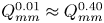 $Q_{mm}^{0.01} \approx Q_{mm}^{0.40}$, which means that the contribution of suspension to the temporal maximum transport rate of momentum almost vanishes. However, in figure 11(b),
 $j_{sm}^{0.01} < j_{sm}^{0.40}$ and
 $j_{mm}^{0.01} < j_{mm}^{0.40}$ are clearly illustrated where
 $L/{h_w} > 0.40$. This indicates a non-zero thickness of suspension at the sections while the contribution of the suspension to the momentum transport rate is minor.
Spatial variations of the temporal maximum (a) transport rates and (b) fluxes of the slide momentum along the propagation path in case A.

3.2. Effects of sediment suspension
Effects of sediment suspension on the variations of the slide translational momentum are further illustrated by examining the results of case B, where no notable sediment suspension was observed in the physical experiment. The temporal variations of the transport rate and flux of slide momentum across the sections of  $L/{h_w} = 0.00,0.15,0.30$ are shown in figure 12. The variations of the temporal maximum transport rate
 $Q_{lm}^{{\alpha _0}}$ and flux
 $j_{lm}^{{\alpha _0}}$ along the propagation are shown in figure 13. In figure 12, without the sediment suspension, the granular momentum transport rates
 $Q_s^{0.01}$ and
 $Q_s^{0.40}$ are almost equal at any time and the differences between
 $Q_m^{0.01}$ and
 $Q_m^{0.40}$,
 $j_s^{0.01}$ and
 $j_s^{0.40}$ and
 $j_m^{0.01}$ and
 $j_m^{0.40}$ are generally insignificant. Besides, different from the case in figures 8(b) and 9(b), there is no double-peak feature in the temporal variations of
 $Q_m^{0.01}$ and
 $j_m^{0.01}$ in the absence of sediment suspension. Figure 14 shows the fields of fluid velocity and sediment concentration at the instants when the peaks of
 $Q_m^{0.01}$ across the sections
 $L/{h_w} = 0.00$ and
 $L/{h_w} = 0.15$ appear. There is no suspension of sediment from the main slide body and the anti-clockwise circulation due to the vertical convection at the slide front is very weak, as observed previously in physical experiments (e.g. Mohammed & Fritz Reference Mohammed and Fritz2012). No second peaks of
 $Q_m^{0.01}$ and
 $j_m^{0.01}$ can be generated by this weak vortex. Furthermore, it is shown in figure 13 that the spatial peaks of
 $Q_{lm}^{{\alpha _0}}$ and
 $j_{lm}^{{\alpha _0}}$ are located at the slope toe. In the weak circulation, the inter-phase drag force is not strong enough to overcome the bottom resistance for an acceleration of the slide. Thus, in figure 13, the temporal maximum transport rate
 $Q_{lm}^{{\alpha _0}}$ and flux
 $j_{lm}^{{\alpha _0}}$ of the slide momentum decrease along the propagation over the flat bottom.
Temporal variations of (a) the transport rates of granular momentum  $Q_s^{0.01}$ and
 $Q_s^{0.40}$, (b) the transport rates of total momentum
 $Q_m^{0.01}$ and
 $Q_m^{0.40}$, (c) the fluxes of granular momentum
 $j_s^{0.01}$ and
 $j_s^{0.40}$ and (d) the fluxes of total momentum
 $j_m^{0.01}$ and
 $j_m^{0.40}$ across the sections at
 $L/{h_w} = 0.00,\;0.15,\;0.30$ in case B.

Spatial variations of the temporal maximum (a) transport rates and (b) fluxes of the slide momentum along the propagation path in case B.

Fluid velocity fields and distribution of sediment concentration at (a)  $T = 5.84$ when the peak of
 $Q_m^{0.01}$ across the section
 $L/{h_w} = 0.00$ appears and (b)
 $T = 6.71$ when there is the peak of
 $Q_m^{0.01}$ across the section
 $L/{h_w} = 0.15$. The red solid and dashed curves are the computed contours of
 ${\alpha _s} = 0.40$ and
 ${\alpha _s} = 0.01$, respectively.

3.3. Effects of slide physical variables
The slide initial acceleration has long been taken as the key parameter of submarine landslides, especially for the generated tsunami (Hammack Reference Hammack1973; Watts Reference Watts1998; Haugen, Løvholt & Harbitz Reference Haugen, Løvholt and Harbitz2005; Heller & Hager Reference Heller and Hager2010; Romano et al. Reference Romano, Lara, Barajas, Di Paolo, Bellotti, Di Risio, Losada and De Girolamo2020). However, for deformable underwater granular landslides, the initial acceleration depends on various physical variables, such as the grain size and the initial compaction, and is not easy to determine. At present, existing formulas of the slide initial acceleration (Romano et al. Reference Romano, Lara, Barajas, Di Paolo, Bellotti, Di Risio, Losada and De Girolamo2020) were proposed for rigid blocks and no convincing formulation for deformable landslides is available. Therefore, rather than considering the initial acceleration, the effects of the specific physical variables of submarine granular landslides, including the initial slide volume  ${V_0}$, the initial height of the slide centroid
 ${h_\textrm{s}}$, the grain size
 ${d_s}$, the initial compaction
 ${\alpha _{s0}}$, the initial slide thickness
 ${s_0}$, the front intrusion angle
 $\beta $ and the initial submergence depth
 ${\varDelta _s}$, on the variations of landslide translational momentum are numerically investigated in the present study. Table 4 lists all the simulation cases and the adopted values of the variables. It is noted that the effects of the grain size, the initial compaction and the front intrusion angle have seldom been intensively examined in existing studies while the grain size and the initial compaction significantly influence the initial acceleration of deformable underwater landslides. For brevity, here, only the effects of these three variables are shown in the figures and discussed in detail. Those of the other variables are involved in the scaling analysis of the following section. It is noted that the present study focuses on submerged monodisperse granular landslides in laboratory experiments. For real landslides composed of visco-plastic soils, the initial yield strength and remoulding rate of the landslide material are dominating parameters and the involved dynamics can be quite different from that in granular landslides (Kim et al. Reference Kim, Løvholt, Issler and Forsberg2019; Zengaffinen-Morris, Urgeles & Løvholt Reference Zengaffinen-Morris, Urgeles and Løvholt2022). Besides, it is also remarked that the initial compaction state of real landslides may be significantly different from that of the artificially prepared landslides in laboratory experiments. Hence, special attention should be paid when extending the present results of initial compaction effects to real landslides.
3.3.1. Effects of grain size
Grain size has shown to be a major determinant in the motion of submerged granular flows (Baumgarten & Kamrin Reference Baumgarten and Kamrin2019; He, Shi & Yu Reference He, Shi and Yu2021) while in previous studies the effects of grain size on the momentum of granular landslides were far from being fully understood or even neglected (Heller & Hager Reference Heller and Hager2010). In this subsection, the effects of grain size on variations of the slide translational momentum are numerically investigated by conducting more simulations of the landslide in case A with different values of sediment diameter  ${d_s}$. The other physical variables and model parameters are kept the same as those in the simulation of case A.
Figure 15 shows the spatial variations of the temporal maximum transport rate and flux of the total momentum of slides with different grain sizes. For the slide with a sediment diameter of 0.2∼1.6 mm, both  $Q_{mm}^{{\alpha _0}}$ and
 $j_{mm}^{{\alpha _0}}$ first increase and then decrease gradually with the propagation distance over the flat bottom. The peaks of
 $Q_{mm}^{{\alpha _0}}$ and
 $j_{mm}^{{\alpha _0}}$ are located away from the slope toe, which indicates an acceleration of the slide over the bottom under the generated anti-clockwise water circulation, as discussed in § 3.1. The contribution of suspension to the slide total momentum is notable with a significant gap between the curves of
 $Q_{mm}^{0.01}$ and
 $Q_{mm}^{0.40}$. However, for the slide with a sediment diameter of 3.0∼4.0 mm,
 $Q_{mm}^{{\alpha _0}}$ decreases immediately behind the slope toe and the contribution of suspension to the slide momentum is negligible. It is shown in figure 15 that the peak values of
 $Q_{mm}^{{\alpha _0}}$ and
 $j_{mm}^{{\alpha _0}}$ generally decrease with increasing grain size, even though when
 ${d_s} = 0.2 \sim 1.6\;\textrm{mm}$ the difference in the peaks of
 $Q_{mm}^{0.40}$ is not great. Moreover, the final run-out of the slide, defined as the position where both
 $Q_{mm}^{{\alpha _0}}$ and
 $j_{mm}^{{\alpha _0}}$ vanish, is clearly shown to increase with the decrease of grain size. For the cases investigated in the present study, off a slope, the submarine granular landslide with a finer grain size has a larger translational momentum, which results in a longer influencing extension and a greater potential impact on underwater infrastructure.
Spatial variations of the temporal maximum (a) transport rates and (b) fluxes of the total momentum along the propagation path of the slides with different grain sizes.

Nonetheless, according to (A12)–(A14), a finer grain size leads to a larger inter-phase drag coefficient (Gidaspow Reference Gidaspow1994), which means that the submarine granular landslide with a finer grain size is subject to a stronger inter-phase drag resistance and hence has a lower initial acceleration. According to existing studies of landslides, a lower initial acceleration may lead to a smaller slide translational momentum. This is contrary to the present results in figure 15. To address the inconsistency, figure 16 exhibits the temporal evolutions of the slide frontal position and the maximum granular velocity parallel to the bed  ${U_{sm}}$. It is shown that a finer grain size indeed leads to a shorter frontal propagation distance and a smaller velocity, but mainly in the accelerating regime of the landslide (before
 ${T \approx 3}$). However, in the later steady regime, a finer grain size does not definitely lead to a lower propagation velocity. On the contrary, when arriving at the slope toe, the computed maximum granular velocity in the slide with
 ${d_s} = 0.2\;\textrm{mm}$ is above 0.60 m s−1, higher than that in the slide with
 ${d_s} = 4.0\;\textrm{mm}$ (approximately 0.46 m s−1). Besides, at the slope toe, the slide with a finer grain size generally has greater values of
 $Q_{mm}^{{\alpha _0}}$ and
 $j_{mm}^{{\alpha _0}}$ as shown in figure 15. This is because the inter-grain shear resistance in the granular slide with a finer grain size is smaller, according to (A5) and (A11), and thus the landslide energy dissipated by the inter-grain shear resistance down the slope is lower. Moreover, on the flat bottom, the slide with a finer grain size is subject to a stronger inter-phase drag force by the generated anti-clockwise water circulation and is easier to accelerate to achieve a higher momentum, as shown in figure 17. Especially in the suspension region and the front part of the slide, it is illustrated in figure 17 that the inter-phase drag force facilitating the slide propagation is notably greater on the grains with
 ${d_s} = 0.8\;\textrm{mm}$ than on those with
 ${d_s} = 3.0\;\textrm{mm}$. The above mentioned inconsistency between the initial acceleration analysis and the present results arises from the hypothesis that a lower initial acceleration leads to a smaller slide translation momentum. The present results demonstrate that the initial acceleration of the slide has a minor effect on the translational momentum of submarine granular landslides off the slope.
Temporal evolution of (a) frontal position and (b) maximum granular velocity parallel to bed of the slides with different grain sizes.

Inter-phase drag force along the propagation direction x on grains,  $f_{s,1}^d$, in the slides with a grain size of (a)
 ${d_s} = 0.8\;\textrm{mm}$ and (b)
 ${d_s} = 3.0\;\textrm{mm}$. The red solid and dashed curves are the computed contours of
 ${\alpha _s} = 0.40$ and
 ${\alpha _s} = 0.01$, respectively.

For more information, the generated leading waves at the slope toe by landslides with different grain sizes are compared in figure 18. The height of the leading wave crest induced by the slide with  ${d_s} = 0.2\;\textrm{mm}$ is the smallest while that by the slide with
 ${d_s} = 4.0\;\textrm{mm}$ is the largest. The amplitude of the generated leading wave increases with the grain size, as depicted by the arrow in figure 18. This is consistent with the analysis of the slide initial acceleration in the above paragraph. As reported in the existing literature, the tsunami height is primarily determined by the momentum transfer from the slide to water in the early accelerating regime and dominated by the slide initial acceleration (Hammack Reference Hammack1973; Heller & Hager Reference Heller and Hager2010; Løvholt et al. Reference Løvholt, Pedersen, Harbitz, Glimsdal and Kim2015; Romano et al. Reference Romano, Lara, Barajas, Di Paolo, Bellotti, Di Risio, Losada and De Girolamo2020). A slide with a finer grain size and hence a smaller initial acceleration generally generates a lower leading wave.
Leading waves at the slope toe  $L/{h_w} = 0$ generated by the slides with different grain sizes. Here,
 $\eta $ is water elevation above the initial level. The arrow depicts that the height of the generated leading wave increases with the grain size.

3.3.2. Effects of initial compaction
The initial compaction of grains plays a key role in underwater collapse of granular materials by virtue of the shear dilatation/contraction (Rondon, Pouliquen & Aussillous Reference Rondon, Pouliquen and Aussillous2011; Bouchut et al. Reference Bouchut, Fernández-Nieto, Mangeney and Narbona-Reina2016; Shi et al. Reference Shi, Dong, Yu and Zhou2021; Rauter et al. Reference Rauter, Viroulet, Gylfadóttir, Fellin and Løvholt2022). Once the collapse starts, a densely packed granular landslide with an initial solid volumetric fraction larger than the critical-state equilibrium concentration experiences shear dilatation, leading to an increase in the frictional inter-grain pressure and shear resistance as well as a decrease in the pore pressure. Those reduce the initial acceleration of the slide and slow down the granular flow. On the contrary, a loosely packed granular landslide with an initial solid volumetric fraction smaller than the equilibrium concentration undergoes shear contraction and has a decrease in inter-grain friction as well as an increase in pore pressure. The shear contraction increases the initial acceleration of the slide and speeds up the landslide propagation. It is noted that the shear dilatation/contraction plays an important role mainly in the accelerating regime of submarine landslides and its effects are more significant in the slides with a finer grain size (Lee & Huang Reference Lee and Huang2021).
The effects of shear dilatation/contraction on submarine granular landslides are captured by the present two-phase model. Numerical results of the frontal position of the slides with different values of initial solid volumetric fraction are shown in figure 19. Comparison of the generated leading waves at the slope toe is shown in figure 20. In the present simulations, the critical-state equilibrium concentration of the granular material is  ${\alpha_{eq} = 0.58}$, as shown in table 6. The initial solid volumetric fraction of the granular slide in case A is
 ${\alpha _{s0}} = 0.60$, corresponding to the shear dilatation case. Here, for comparison, two more cases of the initial compaction
 ${\alpha _{s0}} = 0.56$ and
 ${\alpha _{s0}} = 0.58$ are simulated, respectively corresponding to the shear compaction and equilibrium cases. The other physical variables and model parameters are kept the same with those in the simulation of case A. It is shown in figure 19 that in the accelerating regime the loosely packed granular slide with
 ${\alpha _{s0}} = 0.56$ has the longest propagation distance while the densely packed slide with
 ${\alpha _{s0}} = 0.60$ has the shortest. Correspondingly, in figure 20, the height of the leading wave crest generated by the loosely packed slide is largest. The results are consistent with the analysis of slide initial acceleration in the above paragraph and also with the conclusions of existing related studies (Rondon et al. Reference Rondon, Pouliquen and Aussillous2011; Bouchut et al. Reference Bouchut, Fernández-Nieto, Mangeney and Narbona-Reina2016; Lee et al. Reference Lee, Lo, Shi and Huang2022). It should be noted that in figures 19 and 20 the differences in the results are not huge because the grain size in these cases
 $({d_s} = 0.8\;\textrm{mm)}$ is large.
Temporal evolution of frontal position of the slides with different values of initial compaction.

Leading waves at the slope toe generated by the slides with different values of initial compaction.

In figure 19, after the steady and the deceleration regimes, the densely packed slide has the longest run-out. This shows that the slide final run-out increases with the initial compaction. Further, the effects of initial compaction on the variations of the slide translational momentum over the flat bottom are shown in figure 21. Generally, the values of  $Q_{mm}^{{\alpha _0}}$ and
 $j_{mm}^{{\alpha _0}}$ of a slide with a high initial solid volumetric fraction are larger than those with a low initial compaction. The final run-out measured in terms of the slide momentum increases slightly with the initial compaction, consistent with the results of the slide frontal position shown in figure 19. To illustrate the effects of initial compaction more dramatically, three more cases are simulated with a grain size of
 ${d_s} = 0.2\;\textrm{mm}$. Figure 22 compares the variations of the temporal maximum transport rate and flux of the slide total translational momentum along the propagation. Behind approximately
 $L/{h_w} = 0.5$, the values of
 $Q_{mm}^{{\alpha _0}}$ and
 $j_{mm}^{{\alpha _0}}$ increase significantly with the initial compaction. Before
 $L/{h_w} = 0.50$, the values of
 $Q_{mm}^{{\alpha _0}}$ and
 $j_{mm}^{{\alpha _0}}$ fluctuate dramatically along the propagation path. The fluctuation in the values is due to the strong circulation in the suspension region and the ever-changing shape of the suspension region. The contribution of suspension to the slide total momentum, at the slope toe approximately 76.2 %, 50.7 % and 26.7 % respectively, in the slides of
 ${\alpha _{s0}} = 0.56$,
 ${\alpha _{s0}} = 0.58$ and
 ${\alpha _{s0}} = 0.60$, generally decreases with the initial solid volumetric fraction. Similar to the results in figure 21, the run-out of the slides with
 ${d_s} = 0.2\;\textrm{mm}$ also increases slightly with the initial compaction.
Spatial variations of the temporal maximum (a) transport rates and (b) fluxes of the total momentum along the propagation path of the slides with different values of initial granular volumetric fraction but the same grain size of  ${d_s} = 0.8\;\textrm{mm}$.

Spatial variations of the temporal maximum (a) transport rates and (b) fluxes of the total momentum along the propagation path of the slides with different values of initial granular volumetric fraction but the same grain size of  ${d_s} = 0.2\;\textrm{mm}$.

3.3.3. Effects of the front intrusion angle
The effects of the slide front intrusion angle, i.e.  $\beta $ shown in figure 1, were investigated in only a few studies of subaerial slides (Kamphuis & Bowering Reference Kamphuis and Bowering1972; Heller & Spinneken Reference Heller and Spinneken2013). Its influence on the momentum of deformable submarine landslides has never been studied.
The variations of the temporal maximum transport rates and fluxes of the slide total momentum along the propagation path are shown in figure 23. Here, five different values of the slide front intrusion angle, i.e.  $\beta = 25\mathrm{^\circ },\;30\mathrm{^\circ },\;35\mathrm{^\circ },\;40\mathrm{^\circ },\;45\mathrm{^\circ }$, are adopted. It is noted that, as the inclination of submarine landslides in practice is generally smaller than
 $90\mathrm{^\circ }$, the maximum intrusion angle of the slide is
 $90\mathrm{^\circ } - \theta $. In the cases investigated, the initial mass of granular materials and the height of the granular pile centroid are kept the same with those in case A. All the other physical variables and model parameters are also the same as in the simulation of case A. In figure 23(a), it is shown that the peak values of the total momentum transport rate
 $Q_{mm}^{{\alpha _0}}$ decrease slightly with increasing front intrusion angle. Generally, a larger intrusion angle leads to a greater dynamic pressure resistance on the slide and hence slows down its propagation (Romano et al. Reference Romano, Lara, Barajas, Di Paolo, Bellotti, Di Risio, Losada and De Girolamo2020). However, due to the deformation of granular landslides, the effects of intrusion angle are not as significant as those on subaerial rigid blocks. In figure 23(b), the peak values of the flux, especially those of
 $j_{mm}^{0.40}$ in the main slide body, vary insignificantly with the front intrusion angle. Besides, the final run-out of the slides also varies little in the present considered cases.
Spatial variations of the temporal maximum (a) transport rates and (b) fluxes of the total momentum along the propagation path of the slides with different values of front intrusion angle  $\beta $.

Moreover, figure 24 compares the generated leading waves at the slope toe. Although the wave induced by the slide with a larger front intrusion angle seems to have an earlier and higher crest, the difference in the results is very slight. The present simulated results are consistent with the reported experimental finding that the shape of deformable granular landslides has a minor effect on the generated tsunami (Ataie-Ashtiani & Najafi-Jilani Reference Ataie-Ashtiani and Najafi-Jilani2008).
Leading waves at the slope toe induced by the slides with different values of front intrusionangle  $\beta $.

4. Scaling relations
For the highest impact possible on underwater infrastructure by submarine landslides, a spatial-temporal maximum momentum transport rate  $\varGamma $ and flux
 $\varPhi $ are defined as
 \begin{gather}\varGamma = \mathop {\max }\limits_{L/{h_w} \ge 0} \{Q_{mm}^{0.40}\},\end{gather}
 \begin{gather}\varPhi = \mathop {\max }\limits_{L/{h_w} \ge 0} \{ j_{mm}^{0.40}\} .\end{gather}
Here,  $\varGamma $ and
 $\varPhi $ account for the impact force and the averaged pressure by the main slide body, respectively. It is shown in the figures of § 3 that the momentum flux
 $j_{mm}^{0.40}$ excluding the suspension is generally higher than
 $j_{mm}^{0.01}$. Hence, to estimate the possible highest pressure on infrastructure,
 $j_{mm}^{0.40}$ contributed by the main slide body is considered in the scaling analysis and the component contributed by the suspension is excluded. To keep it consistent with the flux, the transport rate
 $\varGamma $ is also defined without the suspension contribution involved. Further, a slide final run-out in terms of the momentum flux,
 ${L_t}$, is defined as the run-out length from the slope toe to the position where
 $j_{mm}^{0.40}/{\rho _f}g{h_w} = 1\,\%$, expressed as
 \begin{equation}{L_t} = L{|_{j_{mm}^{0.40}/{\rho _f}g{h_w} = 1\,\%}}.\end{equation}
The threshold 1 % adopted here is groundless but it implies a practical application to determining a safe distance away from the slope for submarine infrastructure based on user-defined bearing capacity.
Any property of submarine landslides,  $\varPi $, can be stated as a function of the following variables:
 \begin{equation}\varPi = f({\rho _s},\;{d_s},{\alpha _{s0}},\;{V_0},\;w,\;{s_0},\;\beta ,\;\theta ,\;{h_s},\;{h_w},\;{\varDelta _s},{\mu _0},\;{\rho _f},\;\nu _f^0).\end{equation}
For ease of reading, the definitions of the notations are reviewed and classified in table 2. In the present study, the sensitivities of the landslide translational momentum to  ${d_s}$,
 ${\alpha _{s0}}$,
 ${V_0}$,
 ${s_0}$,
 $\beta $,
 $\theta $,
 ${h_s}$,
 ${h_w}$,
 ${\varDelta _s}$ and
 $\nu _f^0$ are numerically investigated by changing their values while keeping the other variables same with those in case A. A total of 41 cases are simulated and their settings are listed in table 4. The effects of
 ${d_s}$ and
 ${\alpha _{s0}}$ are explored to highlight the significance of grain size and initial compaction on the dynamics of submarine granular landslides. Referring to existing related studies of subaerial landslides (Heller & Hager Reference Heller and Hager2010), the variables
 ${V_0}$,
 ${s_0}$ and
 $\beta $ are adopted to represent the slide shape effects on the translational momentum. Besides, the variables related to problem configuration, i.e.
 $\theta $,
 ${h_s}$,
 ${h_w}$ and
 ${\varDelta _s}$, are selected also following previous work. Here,
 $\nu _f^0$ is altered to emphasize the effects of interstitial viscous fluid on the dynamics of submerged granular landslides. It is noted that the grain size
 ${d_s}$ and the initial compaction
 ${\alpha _{s0}}$ have never been involved in existing scaling analyses for landslides (Heller & Hager Reference Heller and Hager2010; Rauter et al. Reference Rauter, Hobe, Mulligan, Take and Løvholt2021).
Definition and classification of the variables involved in scaling analysis.

In the present numerical study, only the leading wave generated by submarine landslides is considered. Here, the elevation of leading wave crest at the slope toe above the initial water level, symbolized by  ${\eta _c}$, is adopted to quantify the generated wave. Based on the present numerical results and referring to existing studies of subaerial landslides (Heller & Hager Reference Heller and Hager2010; Rauter et al. Reference Rauter, Hobe, Mulligan, Take and Løvholt2021), a scaling analysis on
 $\varGamma $,
 $\varPhi $,
 ${L_t}$ and
 ${\eta _c}$ yields
 \begin{align}\frac{\varGamma
}{{{m_s}g^{\prime}}} &= \frac{\varGamma }{{{\alpha
_{s0}}({\rho _s} - {\rho _f}){V_0}g}} \nonumber\\
&= {f_1}\left({\frac{{18{\rho_f}\nu_f^0{\omega_s}}}{{({\rho_s} -
{\rho_f})gd_s^2}},\;\frac{{{d_s}}}{{{h_w}}},\;\frac{{{\alpha_{s0}}}}{{{\alpha_{eq}}}},\;\sin
\beta ,\;\sin \theta
,\;\frac{{{s_0}}}{{{h_w}}},\;\frac{{{h_s}}}{{{h_w}}},\;\frac{{{\varDelta_s}}}{{{h_w}}},\;{\mu_0}}
\right)\sin (2\theta
),\end{align}
 \begin{align}\frac{\varPhi }{{{\rho _f}g{h_w}}} &= {f_2}\left( {\frac{{{V_0}}}{{wh_w^2}},\;\frac{{18{\rho_f}\nu_f^0{\omega_s}}}{{({\rho_s} - {\rho_f})gd_s^2}},\;\frac{{{d_s}}}{{{h_w}}},\;\frac{{{\alpha_{s0}}}}{{{\alpha_{eq}}}},\;\sin \beta ,\;\sin \theta ,\;\frac{{{s_0}}}{{{h_w}}},\;\frac{{{h_s}}}{{{h_w}}},\;\frac{{{\varDelta_s}}}{{{h_w}}},\;{\mu_0}} \right)\sin (2\theta ),\end{align}
 \begin{align}\frac{{{L_t}}}{{{h_w}}} &= {f_3}\left( {\frac{{{V_0}}}{{wh_w^2}},\;\frac{{18{\rho_f}\nu_f^0{\omega_s}}}{{({\rho_s} - {\rho_f})gd_s^2}},\;\frac{{{d_s}}}{{{h_w}}},\;\frac{{{\alpha_{s0}}}}{{{\alpha_{eq}}}},\;\sin \beta ,\;\sin \theta ,\;\frac{{{s_0}}}{{{h_w}}},\;\frac{{{h_s}}}{{{h_w}}},\;\frac{{{\varDelta_s}}}{{{h_w}}},\;{\mu_0}} \right)\sin (2\theta ),\end{align}
 \begin{align}\frac{{{\eta _c}}}{{{h_w}}} &= {f_4}\left( {\frac{{{V_0}}}{{wh_w^2}},\;\frac{{18{\rho_f}\nu_f^0{\omega_s}}}{{({\rho_s} - {\rho_f})gd_s^2}},\;\frac{{{d_s}}}{{{h_w}}},\;\frac{{{\alpha_{s0}}}}{{{\alpha_{eq}}}},\;\sin \beta ,\;\sin \theta ,\;\frac{{{s_0}}}{{{h_w}}},\;\frac{{{h_s}}}{{{h_w}}},\;\frac{{{\varDelta_s}}}{{{h_w}}},\;{\mu_0}} \right)\sin (2\theta ),\end{align}
in which  ${m_s} = {\alpha _{s0}}{\rho _s}{V_0}$ is the mass of grains in the slide and
 $g^{\prime} = ({\rho _s} - {\rho _f})g/{\rho _s}$, both already defined in § 3.1;
 ${\omega _s}$ is the settling velocity of grains calculated using the Rubey formula. The dimensionless variable
 $18{\rho _f}\nu _f^0{\omega _s}/({\rho _s} - {\rho _f})gd_s^2$ arises from the ratio of the inter-phase drag force to the slide submerged weight, assuming the difference between the velocities of the granular and the fluid phases to be the grain settling velocity. Besides, the effect of grain size in terms of the inter-grain shear resistance is indicated by the dimensionless variable
 ${d_s}/{h_w}$. The effects of shear dilatation/contraction on submarine landslides are represented by
 ${\alpha _{s0}}/{\alpha _{eq}}$, the ratio of the initial compaction to the critical-state equilibrium fraction. The first dimensionless variable in function
 ${f_2}$, i.e.
 ${V_0}/wh_w^2$, is obtained based on the relation of
 $\varPhi \sim \varGamma /w{s_0}$ and it is also involved in function
 ${f_3}$ as
 ${L_t} \sim \varPhi /{\mu _0}{\rho _s}g^{\prime}$. The coefficient
 $\sin (2\theta )$ is obtained considering that the landslide flow is driven by the gravity component along the slope
 $g^{\prime}\sin \theta $ and the translational momentum is the horizontal component (times
 $\cos \theta $) of the slide momentum (Heller & Hager Reference Heller and Hager2010). The other dimensionless variables are determined referring to the existing studies (Heller & Hager Reference Heller and Hager2010; Rauter et al. Reference Rauter, Hobe, Mulligan, Take and Løvholt2021). It is noted that another reason for excluding the suspension contribution to
 $\varGamma $ in the present scaling analysis is the lack of a dominant dimensionless variable for the height of the suspension domain.
Table 5 shows the values of all the dimensionless variables in (4.5)–(4.8). The dependence of  $\varGamma $,
 $\varPhi $,
 ${L_t}$ and
 ${\eta _c}$ on each variable, i.e. the exponent of each term in the equations, is mainly obtained by performing linear regression on the results of corresponding cases in log–log plots. For example, figure 25 shows the linear fitting to determine the dependence on the dimensionless grain size
 ${d_s}/{h_w}$. As the grain size
 ${d_s}$ appears in both
 $18{\rho _f}\nu _f^0{\omega _s}/({\rho _s} - {\rho _f})gd_s^2$ and
 ${d_s}/{h_w}$, before determining the exponent of the term
 ${d_s}/{h_w}$, the dependence of
 $\varPi $ on the fluid viscosity
 $\nu _f^0$ is firstly obtained by fitting the results of cases A, 24 and 25 where the sensitivity on
 $\nu _f^0$ is studied. It is obtained that
 $\varGamma /{m_s}g^{\prime} \sim {[18{\rho _f}\nu _f^0{\omega _s}/({\rho _s} - {\rho _f})gd_s^2]^{ - 0.190}}$,
 $\varPhi /{\rho _f}g{h_w} \sim {[18{\rho _f}\nu _f^0{\omega _s}/({\rho _s} - {\rho _f})gd_s^2]^{ - 0.003}}$,
 ${L_t}/{h_w} \sim {[18{\rho _f}\nu _f^0{\omega _s}/({\rho _s} - {\rho _f})gd_s^2]^{0.129}}$ and
 ${\eta _c}/{h_w} \sim {[18{\rho _f}\nu _f^0{\omega _s}/({\rho _s} - {\rho _f})gd_s^2]^{ - 0.506}}$. Then, in figure 25, the data of
 $\varGamma ^{\prime}/{m_s}g^{\prime}$,
 $\varPhi ^{\prime}/{\rho _f}g{h_w}$,
 ${L^{\prime}_t}/{h_w}$ and
 ${\eta ^{\prime}_c}/{h_w}$ vs.
 ${d_s}/{h_w}$ are linearly fitted in log–log plots, where
 $\varGamma ^{\prime} = \varGamma /{[18{\rho _f}\nu _f^0{\omega _s}/({\rho _s} - {\rho _f})gd_s^2]^{ - 0.190}}$,
 $\varPhi ^{\prime} = \varPhi /{[18{\rho _f}\nu _f^0{\omega _s}/({\rho _s} - {\rho _f})gd_s^2]^{ - 0.003}}$,
 ${L^{\prime}_t} = {L_t}/{[18{\rho _f}\nu _f^0{\omega _s}/({\rho _s} - {\rho _f})gd_s^2]^{0.129}}$ and
 ${\eta ^{\prime}_c} = {\eta _c}/{[18{\rho _f}\nu _f^0{\omega _s}/({\rho _s} - {\rho _f})gd_s^2]^{ - 0.506}}$. It is shown that the values of
 ${R^2}$ of the fitting in figure 25(a–c) are all larger than 0.87. The
 ${R^2}$ value in figure 25(d) for the leading wave elevation is a little small due to the too low absolute values of
 ${\eta _c}$ but still larger than 0.70. Integrating the results of all dependence regression analyses, the scaling relations (4.5)–(4.8) are further specified to be
 \begin{align}\frac{\varGamma }{{{\alpha _{s0}}({\rho _s} - {\rho_f}){V_0}g}} &\approx {N_1}= 1.874{\left[{\dfrac{{18{\rho_f}\nu_f^0{\omega_s}}}{{({\rho_s} - {\rho_f})gd_s^2}}} \right]^{ - 0.190}}{\left({\dfrac{{{d_s}}}{{{h_w}}}} \right)^{ - 0.537}}{\left({\dfrac{{{\alpha_{s0}}}}{{{\alpha_{eq}}}}} \right)^{{n_1}}}\nonumber\\ & \quad \cdot {(\sin \beta )^{ - 0.492}}{(\sin \theta )^{5.055}}{\left({\dfrac{{{s_0}}}{{{h_w}}}} \right)^{0.849}}{\left({\dfrac{{{h_s}}}{{{h_w}}}} \right)^{2.131}}{\left({\dfrac{{{\varDelta_s}}}{{{h_w}}}} \right)^{0.488}}\sin (2\theta ),\end{align}
 \begin{align} \dfrac{\varPhi }{{{\rho _f}g{h_w}}} & \approx {N_2} = 0.433{\left( {\dfrac{{{V_0}}}{{wh_w^2}}} \right)^{0.263}}{\left[{\dfrac{{18{\rho_f}\nu_f^0{\omega_s}}}{{({\rho_s} - {\rho_f})gd_s^2}}} \right]^{ - 0.003}}{\left({\dfrac{{{d_s}}}{{{h_w}}}} \right)^{ - 0.220}}{\left({\dfrac{{{\alpha_{s0}}}}{{{\alpha_{eq}}}}} \right)^{{n_2}}}\nonumber\\ & \quad \cdot {(\sin \beta )^{ - 0.039}}{(\sin \theta )^{2.879}}{\left({\dfrac{{{s_0}}}{{{h_w}}}} \right)^{ - 0.128}}{\left({\dfrac{{{h_s}}}{{{h_w}}}} \right)^{0.561}}{\left({\dfrac{{{\varDelta_s}}}{{{h_w}}}} \right)^{0.207}}\sin (2\theta ), \end{align}
 \begin{align} \dfrac{{{L_t}}}{{{h_w}}} & \approx {N_3} = 5.434{\left({\dfrac{{{V_0}}}{{wh_w^2}}} \right)^{0.408}}{\left[{\dfrac{{18{\rho_f}\nu_f^0{\omega_s}}}{{({\rho_s} - {\rho_f})gd_s^2}}} \right]^{0.129}}{\left({\dfrac{{{d_s}}}{{{h_w}}}} \right)^{ - 0.425}}{\left({\dfrac{{{\alpha_{s0}}}}{{{\alpha_{eq}}}}} \right)^{{n_3}}}\nonumber\\ & \quad \cdot {(\sin \beta)^{0.021}}{(\sin \theta )^{2.188}}{\left({\dfrac{{{s_0}}}{{{h_w}}}} \right)^{ - 0.012}}{\left({\dfrac{{{h_s}}}{{{h_w}}}} \right)^{1.176}}{\left({\dfrac{{{\varDelta_s}}}{{{h_w}}}} \right)^{0.049}}\sin (2\theta), \end{align}
 \begin{align} \dfrac{{{\eta _c}}}{{{h_w}}} & \approx {N_4} = 0.450{\left({\dfrac{{{V_0}}}{{wh_w^2}}} \right)^{0.337}}{\left[{\dfrac{{18{\rho_f}\nu_f^0{\omega_s}}}{{({\rho_s} - {\rho_f})gd_s^2}}} \right]^{ - 0.506}}{\left({\dfrac{{{d_s}}}{{{h_w}}}} \right)^{ - 0.366}}{\left({\dfrac{{{\alpha_{s0}}}}{{{\alpha_{eq}}}}} \right)^{{n_4}}}\nonumber\\ & \quad \cdot {(\sin \beta)^{0.201}}{(\sin \theta )^{2.415}}{\left({\dfrac{{{s_0}}}{{{h_w}}}} \right)^{0.998}}{\left({\dfrac{{{h_s}}}{{{h_w}}}} \right)^{7.775}}{\left({\dfrac{{{\varDelta_s}}}{{{h_w}}}} \right)^{0.646}}\sin (2\theta). \end{align}
It should be noted that the exponents of the initial compaction term  ${\alpha _{s0}}/{\alpha _{eq}}$, i.e.
 ${n_1}$,
 ${n_2}$,
 ${n_3}$ and
 ${n_4}$, vary with the grain size. In cases 6–8 and 32–41, the sensitivities to the initial compaction are investigated for the slides with a grain size of 0.2 mm, 0.4 mm, 0.8 mm, 1.6 mm, 3.0 mm and 4.0 mm. Fitting relations of
 ${n_1}$,
 ${n_2}$,
 ${n_3}$ and
 ${n_4}$ are obtained and expressed together with the
 ${R^2}$ value as
 ${n_1} = 86.43{(1000{d_s}/{s_0})^{ - 1.095}} \!-\! 2.359$ (
 ${R^2} \!= 0.97$),
 ${n_2} = 3.91 \times {10^5}{(1000{d_s}/{s_0})^{ - 6.540}} - 1.133$ (
 ${R^2} = 0.96$),
 ${n_3} = 12.35{(1000{d_s}/{s_0})^{ - 0.127}} - 6.693$ (
 ${R^2} = 0.92$) and
 ${n_4} ={-} 155.50{(1000{d_s}/{s_0})^{ - 1.398}} - 1.927$ (
 ${R^2} = 0.98$). The slide with a finer grain size shows a stronger dependence on the initial compaction. However, it should be noted that the fitting relations of
 ${n_1}-{n_4}$ are based on limited numerical data and only applicable to monodisperse granular slides with a grain size in the range of 0.2–4.0 mm. The initial compaction state of real landslides may be completely different from that of these monodisperse artificially prepared granular blocks. Further experimental and field investigations into the initial compaction effects are suggested.
Linear regression analyses in log–log plots to determine the dependence of (a)  $\varGamma /{\alpha _{s0}}({\rho _s} - {\rho _f}){V_0}g$, (b)
 $\varPhi /{\rho _f}g{h_w}$, (c)
 ${L_t}/{h_w}$ and (d)
 ${\eta _c}/{h_w}$ on the dimensionless grain size
 ${d_s}/{h_w}$. The dots represent the numerical data and the dashed lines are the best-fit curves. The formulas close to the fitting lines show the dependence on the dimensionless grain size according to the slope of the lines. The values of
 ${R^2}$ of the fit are shown.

The values of  ${R^2}$ for the dependence of
 $\varGamma $,
 $\varPhi $,
 ${L_t}$ and
 ${\eta _c}$ on all the terms in (4.9)–(4.12) are listed in table 3. It is illustrated that the goodness of fit for the dependence is generally reasonable, with most of the
 ${R^2}$ values being larger than 0.80. There exist only several exceptions where
 ${R^2}$ is lower than 0.70. The exceptions mostly occur in the cases of pretty weak dependence where the exponent of the corresponding term in (4.9)–(4.12) is less than 0.1 in absolute value. For example,
 ${R^2}$ for the dependence of
 $\varPhi /{\rho _f}g{h_w}$ on
 $18{\rho _f}\nu _f^0{\omega _s}/({\rho _s} - {\rho _f})gd_s^2$ is 0.04 and correspondingly the exponent of the term
 $18{\rho _f}\nu _f^0{\omega _s}/({\rho _s} - {\rho _f})gd_s^2$ in (4.10) is −0.003. Besides,
 ${R^2}$ for the dependence of
 ${L_t}/{h_w}$ on the slide intrusion angle
 $\sin \beta $ is 0.41 and the exponent of the term
 $\sin \beta $ in (4.11) is 0.021.


Values of variables in all simulation cases. The values in bold are the changes relative to case A in the sensitivity study. Note that the mass of grains  ${m_s} = {\alpha _{s0}}{\rho _s}{V_0}$ and the initial submergence of the slide
 ${\varDelta _s}$ are not independent variables.
 ${\varDelta _s}$ varies with the initial shape and position of the slide as well as the water depth.

Values of dimensionless variables in all simulation cases.

 ${N_1}$,
 ${N_2}$,
 ${N_3}$ and
 ${N_4}$ are the results of the scaling relations (4.9)–(4.12). Figure 26 shows the comparisons of
 $\varGamma /{\alpha _{s0}}({\rho _s} - {\rho _f}){V_0}g$ vs.
 ${N_1}$,
 $\varPhi /{\rho _f}g{h_w}$ vs.
 ${N_2}$,
 ${L_t}/{h_w}$ vs.
 ${N_3}$ and
 ${\eta _c}/{h_w}$ vs.
 ${N_4}$. The dashed lines represent the ±20 % error bands. This illustrates that most of the data are within the ±20 % error bands and (4.9)–(4.12) have a good fit to the corresponding numerical data. In the equations, the exponent value of each dimensionless term indicates the degree of dependence on the corresponding physical variable. It shows that
 $\varGamma $,
 $\varPhi $ and
 ${L_t}$ all increase with decreasing grain size
 ${d_s}$. Besides, the momentum flux
 $\varPhi $ has a very weak dependence on the water viscosity
 $\nu _f^0$ and the front intrusion angle
 $\beta $. Moreover, the final run-out of submarine landslides
 ${L_t}$ is insignificantly affected by the slide front intrusion angle
 $\beta $, the initial slide thickness
 ${s_0}$ and the initial submergence
 ${\varDelta _s}$. Among
 $\varGamma $,
 $\varPhi $,
 ${L_t}$ and
 ${\eta _c}$, the dependence of the leading wave crest elevation
 ${\eta _c}$ on the initial compaction is strongest. These scaling relations are preliminary results of the trial to develop practical formulas for estimating the run-out of submarine landslides and the impact on underwater infrastructure in the framework of momentum.
Comparisons of the scaling relation results and the numerical data of the dimensionless (a) spatial-temporal maximum transport rate of slide momentum  $\varGamma /{\alpha _{s0}}({\rho _s} - {\rho _f}){V_0}g$, (b) spatial-temporal maximum momentum flux
 $\varPhi /{\rho _f}g{h_w}$, (c) final run-out away from the slope toe
 ${L_t}/{h_w}$ and (d) elevation of the generated leading wave crest at the slope toe
 ${\eta _c}/{h_w}$. The dashed lines represent the ±20 % error bounds.

It is noted that the scaling relations are proposed based on numerical data of small-scale granular landslides with a uniform grain size in the range of 0.2–4.0 mm. However, in real submarine landslides, the slide body is usually composed of abundant clay-rich visco-plastic soils. It has been reported that the soil initial yield strength and remoulding rate dominate the genesis of tsunami (Kim et al. Reference Kim, Løvholt, Issler and Forsberg2019; Zengaffinen-Morris et al. Reference Zengaffinen-Morris, Urgeles and Løvholt2022). Nevertheless, the yielding and remoulding processes of visco-plastic soils are excluded in the present two-phase model. Besides, the possibly notable difference in the initial compaction states of real landslides and artificially prepared granular materials in laboratory experiments is not taken into account in the present model. The extension of the proposed scaling relations to real submarine landslides needs more work in future studies.
5. Conclusions
In the present study, the translational momentum of deformable submarine landslides off a non-erodible slope is numerically investigated with a two-phase SPH model. In the paper, the model is verified in two laboratory experiments of submarine landslides, one with and the other without significant sediment suspension. By the two-phase model, the momentum of the granular phase and that of the interstitial fluid phase in landslides are resolved, the sum of which is defined as the slide total momentum. After flowing down the slope, the transport rate and flux of the slide translational momentum along the propagation over the horizontal bottom are extensively examined. At any cross-section along the propagation, the transport rate and flux of both the granular and the total momentum first rapidly increase to a maximum and then decrease gradually, implying that the velocity of the slide front part is larger than that of the rear part. In the main slide body where the granular volumetric fraction is larger than 0.40  $({\alpha _s} \ge 0.40)$, the temporal variations of the transport rate and flux of the total momentum are fully consistent with those of the granular momentum, demonstrating a single-peak pattern. However, for the slide outlined by the contour of
 ${\alpha _s} = 0.01$ covering the suspension region, there is a double-peak feature in the temporal variations of the total momentum transport rate and flux while the variations of the granular momentum transport rate and flux still present a single-peak shape. The second peak, lower than the first, is due to the water vortex within the suspension region in the rear part of the slide. The temporal peaks of the momentum transport rate and flux at the slope toe are not always the maximum among those at all the sections along the propagation. The spatial variations of the temporal maximum transport rate and flux of slide momentum at the cross-sections along the propagation path are investigated. The spatial peaks of the temporal maximum momentum transport rate and flux are generally located away from the slope toe due to an acceleration of the slide after it flows down the slope, under the inter-phase drag force exerted by the generated anti-clockwise water circulation. The effects of sediment suspension arising from the slide body on the variations of the slide translational momentum are further studied. This shows that, without the suspension, the double-peak feature in the temporal variations of the total momentum transport rate and flux disappears.
The effects of landslide physical variables, particularly the grain size, the initial compaction and the front intrusion angle, on the variations of slide translational momentum off the slope are numerically examined using the present two-phase model. It is shown that the spatial peaks of the temporal maximum transport rate and flux of the slide total momentum as well as the slide final run-out generally decrease with increasing grain size. Off the slope, the submarine landslide with a finer grain size has a larger translation momentum, which results in a longer run-out and a greater potential impact on underwater infrastructure. The mechanism analysis exhibits that the initial acceleration of the slide, which has been widely taken as a key governing parameter of landslide-generated tsunami, has a minor effect on the slide translational momentum off the slope. Regarding the effects of the slide initial compaction, a loosely packed granular landslide has a quicker propagation in the accelerating regime and generates a higher leading wave than a densely packed slide. Nevertheless, off the slope, a densely packed granular landslide has a higher translational momentum and a longer final run-out. The temporal maximum transport rate and flux of the slide total momentum as well as the final run-out generally increase with the initial compaction in the slide while the contribution of sediment suspension to the slide total translational momentum decreases with the initial compaction. It is noted that the significance of the initial compaction effects increases with decreasing grain size. Furthermore, a minor effect of the slide front intrusion angle on the peak values of the total translational momentum flux, the slide final run-out and the generated leading wave height is demonstrated in the study.
Based on the numerical results, a scaling analysis on the factors of the slide translational momentum is conducted and scaling relations of the spatial-temporal maximum transport rate and flux of the total translational momentum, the slide final run-out and the generated leading wave crest elevation at the slope toe are proposed. These scaling relations demonstrate the degree of dependence of the slide translational momentum, the final run-out and the tsunami height on physical variables of submerged granular landslides. It is noted that the scaling relations are proposed based on numerical data of small-scale monodisperse granular landslides with a grain size of 0.2–4.0 mm. The visco-plastic rheology of clay-rich soils in real landslides and the difference in the initial compaction state of real landslides and artificially prepared granular materials are neglected in the utilized numerical model. However, the proposed scaling relations still present a preliminary trial to develop practical formulas in the framework of momentum for submarine landslide run-out and the potential impact on underwater infrastructure.
Declaration of interests
The authors report no conflict of interest.
Funding
The authors thank Dr H. Liu from Zhejiang University for the valuable discussion and suggestions. They also appreciate Dr S.T. Grilli's kindness in sharing the experimental data. The research is jointly funded by the National Natural Science Foundation of China (NSFC) under grant No. 12102493, the Science and Technology Development Fund, Macau S.A.R. (File no. 0009/2021/A, SKL-IOTSC(UM)-2021-2023) and Southern Marine Science and Engineering Guangdong Laboratory (Zhuhai) (SML2021SP305). CORE is a joint research centre for ocean research between QNLM and HKUST.
Appendix A
Closures of the two-phase continuity and momentum equations and a minimum description of the adopted two-phase SPH model.
For the fluid phase, the tensor  ${\boldsymbol{\sigma }_f}$ in the momentum equation (2.2) includes the kinetic and the turbulent shear stresses and is expressed by
 \begin{equation}{\sigma _{f,ij}} = 2{\rho _f}(\nu _f^0 + \nu _f^t){S_{f,ij}},\end{equation}
where  $\nu _f^0$ and
 $\nu _f^t$ are respectively the kinematic and the turbulent viscosities of the fluid and
 $\boldsymbol{S}$ is the rate-of-strain tensor, calculated by
 \begin{equation}{S_{k,ij}} = \frac{1}{2}\left( {\frac{{\partial {u_{k,i}}}}{{\partial {x_j}}} + \frac{{\partial {u_{k,j}}}}{{\partial {x_i}}}} \right) - \frac{1}{3}\frac{{\partial {u_{k,l}}}}{{\partial {x_l}}}{\delta _{ij}}.\end{equation}
For the solid particle phase, the stress tensor  ${\boldsymbol{\sigma }_s}$ in (2.2) consists of inter-grain stresses resulting from collisions and enduring contacts among the granular particles. It is estimated by
 \begin{equation}{\sigma _{s,ij}} = 2{\rho _s}(\nu _s^0 + \nu _s^t){S_{s,ij}} - {p_s}{\delta _{ij}},\end{equation}
in which  $\nu _s^0$ is the granular viscosity and
 $\nu _s^t$ is the turbulent viscosity of the granular phase due to the turbulence in the interstitial fluid. The turbulent viscosities of the two phases
 $\nu _k^t$ are evaluated by a modified Smagorinsky model, shown as
 \begin{equation}\nu _k^t = 2{({C_{S,k}}\varDelta )^2}|{\boldsymbol{S}_k}|{\left( {1 - \frac{{{\alpha_s}}}{{{\alpha^ \ast }}}} \right)^5},\end{equation}
where  ${C_S}$ is the Smagorinsky coefficient and
 ${C_{S,f}} = {C_{S,s}} = 0.1$ is adopted in this study;
 $\varDelta $ is the size of the SPH particles utilized in solving the equations;
 $|{\boldsymbol{S}_k}|= \sqrt {{S_{k,ij}}{S_{k,ij}}/2} $ is the norm of the rate-of-strain tensor;
 ${\alpha ^ \ast }$ is the random close-packing volume fraction of the granular materials.
A friction-rheology constitutive law of granular flows is utilized to describe the motion of granular landslides, i.e. to estimate the inter-grain pressure  ${p_s}$ and the granular viscosity
 $\nu _s^0$ (Shi et al. Reference Shi, Dong, Yu and Zhou2021). In the law, the granular viscosity depends on the inter-grain pressure according to a
 $\mu ({I_m})$ relation, shown as
 \begin{gather}\nu _s^0 = \frac{{\mu {p_s}}}{{2{\rho _s}|{\boldsymbol{S}_s}|}};\end{gather}
 \begin{gather}\mu = {\mu _1} + \frac{{{\mu _2} - {\mu _1}}}{{1 + \sqrt {{I_0}/{I_m}} }},\end{gather}
where  $\mu $ is the friction coefficient;
 ${\mu _1} = \tan \phi $ is the granular static friction coefficient and
 $\phi $ is the internal friction angle of the solid materials;
 ${\mu _2} = \tan \phi \sim 1.0$ is the friction coefficient when
 ${I_m}$ is infinite;
 ${I_0}$ is a coefficient.
 ${I_m}$ is a dimensionless number of immersed granular flows and defined as
 \begin{equation}{I_m} = \frac{{2|{\boldsymbol{S}_s}|({\rho _f}\nu _f^0 + 2{c_1}{\rho _s}d_s^2|{\boldsymbol{S}_s}|)}}{{{p_s}}},\end{equation}
in which  ${d_s}$ is the grain diameter;
 ${c_1}$ is a coefficient and
 ${c_1} = 0 \sim 1.0$. The inter-grain pressure
 ${p_s}$ is composed of two components
 \begin{equation}{p_s} = p_s^e + p_s^c.\end{equation}
Here,  $p_s^e$ is the component of inter-grain pressure caused by enduring contacts among solid particles and
 $p_s^c$ is the other component arising from collisions between particles. The formulation integrating the frictional shear dilatation/contraction effects proposed by Shi et al. (Reference Shi, Dong, Yu and Zhou2021) is adopted for
 $p_s^e$
 \begin{equation}p_s^e = p_{s0}^e {\rm exp} \left[ {{c_2}K\frac{{\chi {\alpha_s}}}{{{\alpha_s} - {\alpha_\ast }}}I_d^{{c_3}}({\alpha_s} - {\alpha_{eq}})} \right],\end{equation}
where  $p_{s0}^e$ is the frictional solid pressure excluding the frictional shear dilatation/contraction effect and is estimated by (Hsu, Jenkins & Liu Reference Hsu, Jenkins and Liu2004)
 \begin{equation}p_{s0}^e = \left\{ {\begin{array}{*{20}{@{}l}} 0&{{\alpha_s} \le {\alpha_\ast }}\\ {G{{({\alpha_s} - {\alpha_\ast })}^\chi }\left[ {1 + \sin \left( {\dfrac{{{\alpha_s} - {\alpha_ \ast }}}{{{\alpha^ \ast } - {\alpha_ \ast }}}{\rm \pi} - \dfrac{\rm \pi}{2}} \right)} \right]}&{{\alpha_s} > {\alpha_\ast }} \end{array}} \right.;\end{equation}
where  ${I_d}$ is a non-dimensional shear rate, defined as
 ${I_d} \equiv 2{d_s}|{\boldsymbol{S}_s}|/\sqrt {p_{s0}^e/{\rho _s}} $; K is a material parameter for shear dilatation/contraction and varies in the range of
 $1.0 \sim 25.0$;
 $\chi $ is a parameter to characterize the arrangement of contact force chains among the grains and varies between 1.5 and 5.5;
 ${\alpha _{eq}}$ is the critical-state equilibrium concentration of the granular materials; G is the material parameter for the compressibility of the grains;
 ${\alpha _ \ast }$ is the random loose packing volume fraction of the granular materials;
 ${c_2}$ and
 ${c_3}$ are coefficients. Generally,
 ${c_2} = 0 \sim O(10)$ and
 ${c_3} = 0 \sim 1$ (Shi et al. Reference Shi, Dong, Yu and Zhou2021). The shear-rate-dependent collisional inter-grain pressure
 $p_s^c$ is estimated using the formulation proposed by Trulsson, Andreotti & Claudin (Reference Trulsson, Andreotti and Claudin2012)
 \begin{equation}p_s^c = 2{\left( {\frac{{{c_4}{\alpha_s}}}{{{\alpha^0} - {\alpha_s}}}} \right)^2}({\rho _f}\nu _f^0 + 2{c_1}{\rho _s}d_s^2|{\boldsymbol{S}_s}|)|{\boldsymbol{S}_s}|,\end{equation}
in which  ${\alpha ^0}$ is the jamming volume fraction of the granular materials;
 ${c_4}$ is a coefficient and generally
 ${c_4} = 0 \sim 3.0$.
The inter-phase drag force is estimated by the formula of Gidaspow (Reference Gidaspow1994), shown as
 \begin{gather}f_{s,i}^d ={-} f_{f,i}^d = {\alpha _s}\gamma ({u_{f,i}} - {u_{s,i}}),\end{gather}
 \begin{gather}\gamma = \left\{ {\begin{array}{*{20}{@{}l}} {\dfrac{3}{4}{C_D}\dfrac{{{\rho_f}|{\boldsymbol{u}_f} - {\boldsymbol{u}_s}|}}{{{d_s}}}\alpha_f^{ - 1.65}}&{{\alpha_s} \le 0.2}\\ {150\dfrac{{{\alpha_s}{\rho_f}\nu_f^0}}{{{\alpha_f}d_s^2}} + 1.75\dfrac{{{\rho_f}|{\boldsymbol{u}_f} - {\boldsymbol{u}_s}|}}{{{d_s}}}}&{{\alpha_s} > 0.2} \end{array}} \right.,\end{gather}
 \begin{gather}{C_D} = \left\{ {\begin{array}{*{20}{@{}l}} {\dfrac{{24}}{{R{e_s}}}(1.0 + 0.15Re_s^{0.687})}&{R{e_s} < 1000}\\ {0.44}&{R{e_s} \ge 1000} \end{array}} \right.,\end{gather}
where  ${C_D}$ is the drag coefficient;
 $R{e_s}$ is the particle Reynolds number, defined as
 $R{e_s} \equiv {\alpha _f}|{\boldsymbol{u}_f} - {\boldsymbol{u}_s}|{d_s}/\nu _f^0$.
The detailed SPH formulation of the controlling equations and the numerical implementation of the model can be found in Shi et al. (Reference Shi, Yu and Dalrymple2017, Reference Shi, Si, Dong and Yu2019). The predictor–corrector time-integration scheme is adopted to solve the controlling equations. The simulation time step is restricted by the fluid numerical sound speed assumed in the weakly compressible SPH method, the maximum acceleration of the fluid and the solid phases, and the total viscosity of the two phases, according to the Courant–Friedrichs–Lewy (CFL) conditions
 \begin{gather}\varDelta t \le \min (\varDelta {t_1},\;\varDelta {t_2},\;\varDelta {t_3}),\end{gather}
 \begin{gather}\varDelta {t_1} = 0.3\frac{h}{{\max ({c_s})}},\end{gather}
 \begin{gather}\varDelta {t_2} = 0.3\min \left( {\sqrt {\frac{h}{{\max |{\boldsymbol{a}_f}|}}} ,\sqrt {\frac{h}{{\max |{\boldsymbol{a}_s}|}}} } \right),\end{gather}
 \begin{gather}\varDelta {t_3} = 0.125\min \left( {\frac{{{h^2}}}{{\max ({\nu_f})}},\frac{{{h^2}}}{{\max ({\nu_s})}}} \right),\end{gather}
where  $\varDelta {t_1}$,
 $\varDelta {t_2}$ and
 $\varDelta {t_3}$ are the time steps respectively restricted by the numerical sound speed, the inertia forces and the viscous forces of the two phases;
 ${c_s}$ is the numerical sound speed of the fluid, depending on the fluid pressure;
 $h = 1.3\varDelta $ is the smoothing length utilized in SPH methods;
 ${\boldsymbol{a}_f} = \textrm{d}{\boldsymbol{u}_f}/\textrm{d}t$ is the acceleration of the fluid phase and
 ${\boldsymbol{a}_s} = \textrm{d}{\boldsymbol{u}_s}/\textrm{d}t$ is the acceleration of the solid phase;
 ${\nu _f} = \nu _f^0 + \nu _f^t$ is the fluid total viscosity and
 ${\nu _s} = \nu _s^0 + \nu _s^t$ is the total viscosity of the solid phase.
Appendix B
Set-up of the numerical simulations in the validation cases.
It was noted in Pilvar et al. (Reference Pilvar, Pouraghniaei and Shakibaeinia2019) and Grilli et al. (Reference Grilli, Shelby, Kimmoun, Dupont, Nicolsky, Ma, Kirby and Shi2017) that the sidewalls of the laboratory flume had a negligible influence on the flow at the middle section. In the model validation, physical variables of the water and the slides along the flume centreline were adopted for comparisons. Hence, in the numerical simulations, the landslide–water flows were taken as two-dimensional to reduce the computational effort. The present used two-phase SPH model is a three-dimensional one. For two-dimensional cases, in the simulations the periodic condition was applied in the width direction of the flume.
In the model, the granular–water mixture, the flume bottom, the inclined slope and the sidewall at the downstream end were all represented by SPH particles. Figure 27 shows the initial layout of SPH particles in the simulation of the experiment conducted in Pilvar et al. (Reference Pilvar, Pouraghniaei and Shakibaeinia2019). The dynamic boundary condition in Crespo, Gómez-Gesteira & Dalrymple (Reference Crespo, Gómez-Gesteira and Dalrymple2007) and Shi et al. (Reference Shi, Yu and Dalrymple2017) was utilized in which four layers of SPH particles were used to represent the solid boundaries (i.e. the flume bottom, the inclined slope and the downstream-end wall of the flume). The physical variables carried by the particles for solid boundaries also satisfied the controlling equations of the model, like those in the particles for the granular–water mixture, but these boundary particles are kept fixed in position during the simulations. The dynamic boundary condition has been shown to be effective in representing the interaction between fluid and solid boundaries (Crespo et al. Reference Crespo, Gómez-Gesteira and Dalrymple2007; Shi et al. Reference Shi, Yu and Dalrymple2017). No outlet boundary conditions at the downstream end of the flume were needed.
Initial layout of the SPH particles representing the granular–water mixture and solid boundaries in the simulation of Pilvar et al. (Reference Pilvar, Pouraghniaei and Shakibaeinia2019) experiment (case A).

Along the width of the flume, four layers of SPH particles (including all those representing the granular–water mixture, the inclined slope, the flume bottom and the downstream-end wall) were arranged to implement the periodic condition in the y direction (Shi et al. Reference Shi, Yu and Dalrymple2017), as shown in the upper part of figure 27. In the simulations, the initial size of SPH particles was set to be  $\varDelta = 2\;\textrm{mm}$ based on a convergence study. In the numerical model for the experiment of Pilvar et al. (Reference Pilvar, Pouraghniaei and Shakibaeinia2019) (case A in the main text), a total number of 131 084 SPH particles were utilized, of which 7664 were for the solid boundaries. In the model for the experiment of Grilli et al. (Reference Grilli, Shelby, Kimmoun, Dupont, Nicolsky, Ma, Kirby and Shi2017) (case B in the main text), to reduce the computational effort, the flat bottom of the flume was shortened to be 1.100 m without affecting the propagation of the slide. Accordingly, a total number of 353 100 SPH particles were adopted to represent the granular–water mixture and the solid boundaries.
Based on the criteria described in Appendix A, a fixed time up of  $\varDelta t = {10^{ - 6}}\;\textrm{s}$ was set in the simulations. Values of the model parameters are summarized in table 6.
Values of model parameters adopted in the simulations.


 Open access

