1. INTRODUCTION
Global Satellite Navigation Systems (GNSS) have made signifi-cant progresses in recent years (Jiang et al., Reference Jiang, Xu, Xu, Xu, Sun and Schuh2017; Gioia and Borio, Reference Gioia and Borio2016; Torre and Caporali, Reference Torre and Caporali2015; Jin et al., Reference Jin, Feng and Gleason2011). China's BeiDou satellite navigation system (BDS) and Europe's Galileo satellite navigation system are developing rapidly towards their full operational capability. Twenty-three BeiDou satellites and eighteen Galileo satellites are now orbiting the Earth. BDS has provided regional navigation and positioning services since 27 December 2012 (Jin et al., Reference Jin, Qian and Wu2017). The European Commission formally announced Galileo initial services on 15 December 2016. Both BeiDou and Galileo systems are expected to provide global navigation services with complete constellations by 2020. With the significant progress of BeiDou and Galileo system development, as well as the ongoing Global Positioning System (GPS) and Global Navigation Satellite System (GLONASS) modernisations, multi-GNSS integration has attracted increasing interest. Improved accuracy and reliability of navigation solutions can be expected with the joint use of multiple satellite systems, especially in poor satellite visibility environments, such as in urban canyons, surface mines, forests, and so on.
Although GPS, GLONASS, BeiDou and Galileo systems are quite similar, they adopt different time scales, which causes a bias between measurements from different constellations. In addition, the hardware delay at the receiver is also different for each satellite system. These Inter-System Biases (ISBs) must be properly handled in multi-GNSS integrated navigation so that multi-constellation signals can be used successfully together. A traditional approach to solve this issue is to introduce an additional unknown parameter to estimate the ISB (Angrisano et al., Reference Angrisano, Gaglione and Gioia2013; Chen et al., Reference Chen, Xiao, Zhang and Wu2013; Cai et al., Reference Cai, Luo, Liu and Xiao2014; Choi et al., Reference Choi, Cho, Cho and Lee2015; Pan et al., Reference Pan, Cai, Santerre and Zhang2016). For quad-constellation integrated navigation, this will require at least seven unknown parameters to obtain a navigation solution in a single epoch (Pan et al., Reference Pan, Cai, Santerre and Zhang2016), namely three coordinate components, one receiver clock offset and three ISBs. In order to estimate the three ISB unknown parameters, an extra three satellites from corresponding constellations are required, which limits the navigation applications in a poor satellite visibility environment. Based on the ISBs’ short-term stability characteristics (Cai and Gao, Reference Cai and Gao2008; Jiang et al., Reference Jiang, Xu, Xu, Xu, Sun and Schuh2017), Cai and Gao (Reference Cai and Gao2009) proposed that the ISB could be estimated as an unknown parameter when enough satellites were available, while the latest computed ISB value could be used as a quasi-observable to obtain a position solution in conditions of limited satellite visibility. However, this algorithm requires a threshold value to distinguish if the number of visible satellites is sufficient or insufficient, which is sometimes difficult to determine. Gioia and Borio (Reference Gioia and Borio2016) proposed a similar algorithm to exploit the previous estimates of the ISB parameters as pseudo-measurements, which were updated according to the satellite geometric conditions, i.e. Dilution Of Precision (DOP).
In this study, we first investigate the ISBs’ temporal variation characteristics using datasets spanning nearly three years. Then, an enhanced navigation algorithm is developed to obtain a position solution without sacrificing satellite observations for solving the ISBs. This algorithm does not rely on the threshold values of numbers of satellites or DOP. Finally, some test results are presented.
2. TEMPORAL VARIATION CHARACTERISTICS OF INTER-SYSTEM BIAS
2.1. Daily Variation of GNSS System Time Difference
Different GNSS systems adopt different time scales. Specifically, GPS employs GPS Time (GPST), which is established by GPS master control stations and connected to Coordinated Universal Time (UTC) maintained at the US Naval Observatory (USNO). It is a continuous time system without leap seconds, but has an integer number of seconds and a tiny difference within 1 μ s to UTC (USNO) (ICD-GPS, 2013). The GLONASS system adopts GLONASS Time (GLONASST), which is generated on the basis of a GLONASS central synchroniser. GLONASST is a non-continuous time system since an integer number of seconds are periodically corrected to the GLONASST in order to remain synchronous with UTC (SU) as maintained by Russia (SU stands for the former Soviet Union) (ICD-GLONASS, 2008). BeiDou uses BDS Time (BDT), which is referenced to UTC maintained at the National Time Service Centre (NTSC), Chinese Academy of Sciences. Similar to the GPST, it is a continuous time system without leap seconds (ICD-BDS, 2012). Galileo adopts Galileo System Time (GST), which directly relates to the International Atomic Time (TAI) and differs from GPST in the order of tens of nanoseconds (Gioia and Borio, Reference Gioia and Borio2016). In summary, GPS, GLONASS, BeiDou and Galileo systems adopt different system times maintained by different atomic clocks. Due to the differences of the atomic clocks and data processing methods, these system times differ by amounts varying from a tiny fractional second to an integer numbers of seconds.
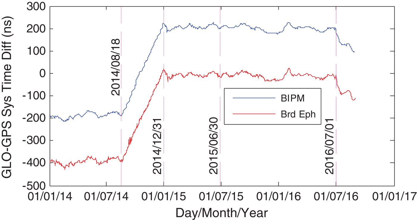
The Time Department of the Bureau International des Poids et Mesures (BIPM) routinely releases time synchronisation products between GPST and UTC as well as GLONASST and UTC, which can be used to calculate the GLONASS-GPS system time differences. The analogous products for BDS and Galileo are not yet available from the BIPM. On the other hand, the GLONASS-GPS system time differences have been disseminated via broadcast ephemerides at an updating interval of one or two days. Similarly, Galileo-GPS system time differences have been broadcast since 2 May 2013. However, BDS-GPS system time differences are not yet available from broadcast ephemerides. Since only GLONASS-GPS system time differences are available from both the BIPM and broadcast ephemerides, the BIPM-derived GLONASS-GPS system time differences are compared with those obtained from the broadcast ephemerides. Figure 1 shows the daily variations of the GLONASS-GPS system time differences acquired from the two different sources from 1 January 2014 to 31 August 2016. The blue line represents the time difference series from the BIPM products while the red line represents the ones from the broadcast ephemerides with a file name pattern of “brdmdddf.yyp”. It can be seen that the blue line exhibits a similar variation to the red line but there is an offset of about 210 ns between them. From 1 January 2015 to 1 July 2016, the daily variations of the time difference series are stable with a Standard Deviation (STD) of less than 7 ns. However, it is interesting to note that the time difference series linearly increases from 18 August – 31 December 2014. This is because of a procedure for GLONASST correction to minimise the offset of GLONASST relative to UTC(SU) (Bogdanov et al., Reference Bogdanov, Druzhin, Primakina and Tiuliakov2015). It appears that a decreasing tendency started on 1 June 2016. From the perspective of long-term variation, the GLONASS-GPS system time difference series are not stable. A UTC leap second event actually occurred on 30 June 2015, but from Figure 1, the GLONASS-GPS system time differences do not show any abrupt leap on that day, which suggests that the leap seconds have been removed from both sources.
GLONASS-GPS system time differences from 1 January 2014 to 31 August 2016.

2.2. Temporal Variation of Inter-System Bias
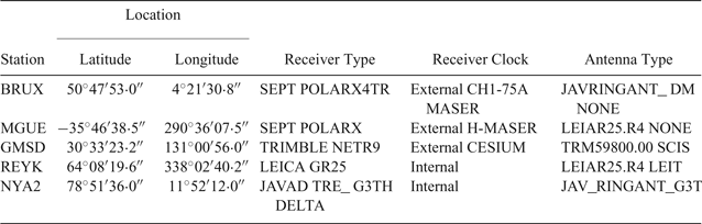
In addition to the system time differences between different GNSS systems, the ISB still contains the code hardware delay biases, which are different for different satellite systems (Jin et al., Reference Jin, Jin and Li2016). To investigate its temporal variations, the ISB is estimated as an unknown parameter along with Three-Dimensional (3D) receiver coordinates and one receiver clock offset using the least square method. The datasets at five Multi-GNSS Experiment (MGEX) stations, namely BRUX, GMSD, MGUE, REYK and NYA2, from 1 January 2014 to 31 August 2016 are used for the ISB computation. The receiver types, receiver clock and antenna types at these stations are listed in Table 1. As most GPS/GLONASS/BDS/Galileo navigation users use single-frequency receivers, only the code measurements on the L1/G1/B1/E1 frequency bands are utilised in this study. The observations have a sampling rate of 30 s with an elevation mask angle of 10°.
Receiver and antenna types.

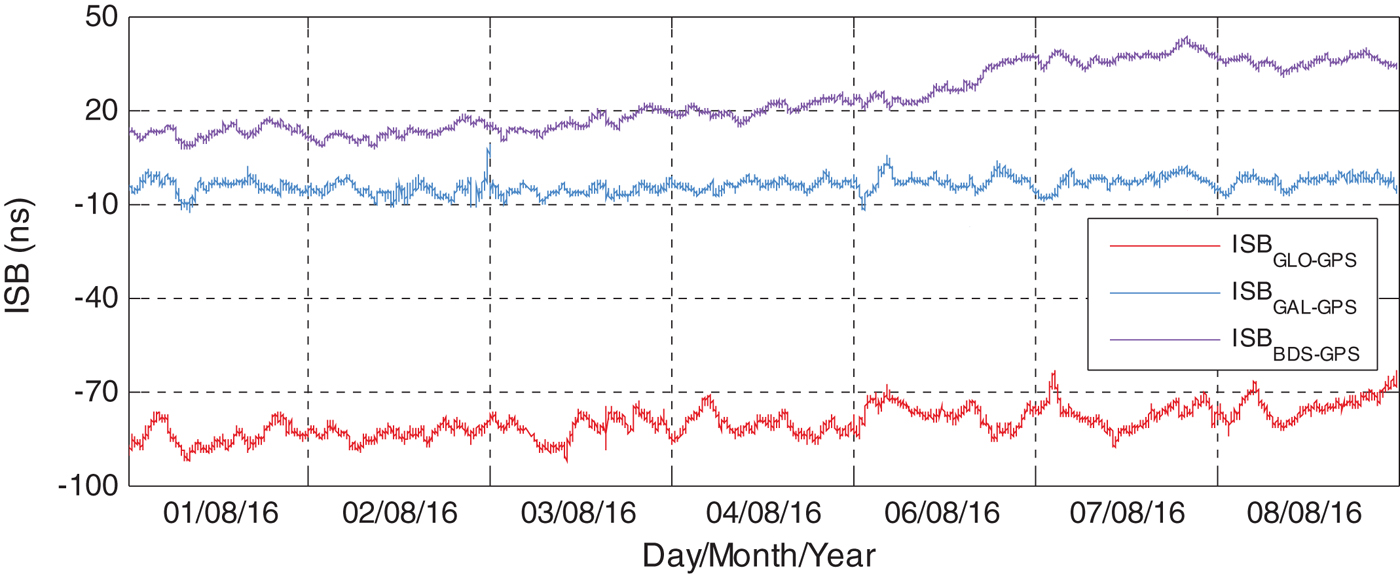
To examine ISB short-term stability, station coordinates, receiver clock offset and ISBs are estimated on an epoch-by-epoch basis using the quad-constellation single point positioning method (Pan et al., Reference Pan, Cai, Santerre and Zhang2016). The epoch-wise GLONASS-GPS, BDS-GPS and Galileo-GPS ISB estimates at GMSD from 1 August 2016 to 8 August 2016 are displayed in Figure 2. The dataset on 5 August 2016 was not processed due to lack of observation data. The number of visible BDS or Galileo satellites was over three at GMSD on these days. The ISB estimates are stable within one day with standard deviations smaller than 4 ns, 5 ns and 3 ns for GLONASS-GPS, BDS-GPS and Galileo-GPS ISBs, respectively. The estimated Galileo-GPS ISBs are consistent in magnitude with the reported results in Gioia and Borio (Reference Gioia and Borio2016).
ISB series at GMSD from 1 August 2016 to 8 August 2016.

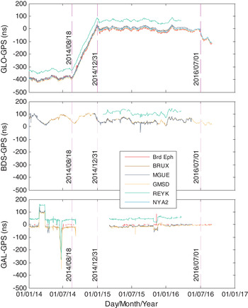
To examine the ISB long-term stability, Figure 3 shows the epoch-average ISB estimates between GPS and other GNSS systems for each day from 1 January 2014 to 31 August 2016. For comparison purposes, the GLONASS-GPS and Galileo-GPS system time differences derived from the broadcast ephemerides are also plotted. The GLONASS-GPS ISB series are highly consistent with the GLONASS-GPS system time difference series with an average correlation coefficient of 99·97%. The high correlation of GLONASS-GPS ISB and system time difference series suggests that the ISB is mainly affected by the system time differences. Due to the larger fluctuation caused by the lower number of Galileo satellites and the absence of system time difference information for some days in the broadcast ephemeris, the correlation for Galileo-GPS was not calculated. Likewise, the correlation for BDS-GPS was not available since its system time difference information had not yet been broadcast. For different stations, the ISB series has offsets, especially for the station REYK. This is because of the existence of hardware delay biases, which differ from different receiver and antenna types (Cai and Gao, Reference Cai and Gao2009). It is noted that a few daily jumps occur at the MGUE station. This is because of the lower number of BeiDou satellites at the South American station. As seen from Figure 3, the GLONASS-GPS ISBs are down to about −400 nanoseconds. The absolute values of the BDS-GPS and Galileo-GPS ISBs are relatively smaller reaching several tens of nanoseconds. Therefore, the ISBs cannot be ignored in multi-GNSS integrated navigation.
ISB estimates between GPS and other GNSS systems from 1 January 2014 to 31 August 2016.

3. ENHANCED MULTI-GNSS NAVIGATION ALGORITHM
In the traditional multi-GNSS navigation algorithm, the ISB is estimated as an unknown parameter when the number of GNSS satellites is sufficient. However, three ISB unknown parameters will be required in quad-constellation combined navigation. As a result, three additional satellites from the corresponding constellations will be essential to solve the three unknown ISB parameters. Under limited satellite visibility situations, observations from the three satellites could be vital in obtaining a navigation solution. In order to avoid sacrificing GNSS observations, an enhanced multi-GNSS navigation algorithm is developed in this section.
Since GPS, GLONASS, BeiDou and Galileo systems have their respective time systems, a receiver clock parameter with respect to its own time scale should be introduced for each constellation although there is a unique physical receiver clock (Cai et al., Reference Cai, Gao, Pan and Zhu2015). Alternatively, system time difference parameters with respect to a reference time scale may be introduced (Cai and Gao, Reference Cai and Gao2013). If the GPS time scale is chosen as the reference, the quad-constellation observation model is described by:
 $$P^{g} = \rho^{g} + cdT - cdt^{g} + d_{orb}^g + d_{trop}^g + d_{ion}^g + \varepsilon_{P}^g$$
 $$P^{i} = \rho^{i} + cdT - cdt^{i} + ISB^i + d_{orb}^i + d_{trop}^i + d_{ion}^i + \varepsilon_{P}^i$$
 $$B^i = ISB^i + \varepsilon_{B}^i$$
where the superscript g represents a GPS satellite, i represents GLONASS, BeiDou and Galileo satellites, P is the code observation, B is the a priori ISB, ρ is the geometric distance between the satellite and the receiver, c represents the speed of light in a vacuum, dT is the GPS receiver clock offset and dt is the satellite clock offset, ISB is the inter-system bias with respect to the GPS system, including the system time difference and hardware delay bias, d orb is the satellite orbit error, d trop is the tropospheric delay, d ion is the ionospheric delay and, ε contains the un-modelled errors, multipath and measurement noise.
Broadcast ephemerides are used to calculate the satellite position and the satellite clock offset. Although the four GNSS systems employ different coordinate references, their differences are at a level of only a few centimetres (Montenbruck et al., Reference Montenbruck, Steigenberger and Hauschild2015; Torre and Caporali, Reference Torre and Caporali2015). Such a small difference may be neglected in metre-level navigation solutions. The tropospheric delay is corrected using the Saastamoinen model (Saastamoinen, Reference Saastamoinen1973) with an input of standard meteorological data. The NeQuick model (Nava et al., Reference Nava, Coisson and Radicella2008; Oladipo and Schüler, Reference Oladipo and Schüler2012) is adopted for Galileo ionospheric delay corrections while the Klobuchar model (Klobuchar, Reference Klobuchar1987) is utilised for the ionospheric delay corrections of GPS, GLONASS and BeiDou observations. Time group delays provided in the broadcast navigation messages are applied to correct the satellite hardware delay biases. The least square method is used to estimate the unknown parameters of three coordinate components, one receiver clock offset and three ISBs. The code observations are weighted with satellite elevation angles (Pan et al., Reference Pan, Cai, Santerre and Zhang2016) but different initial weights are assigned to different GNSS systems. The initial weight ratios of GPS, GLONASS, BeiDou and Galileo observations are set to 2:1:2:1 (Pan et al., Reference Pan, Cai, Santerre and Zhang2016). That is to say, the precisions of GPS, GLONASS, BeiDou and Galileo code observations are set to 0·3 m, 0·6 m, 0·3 m and 0·6 m, respectively.
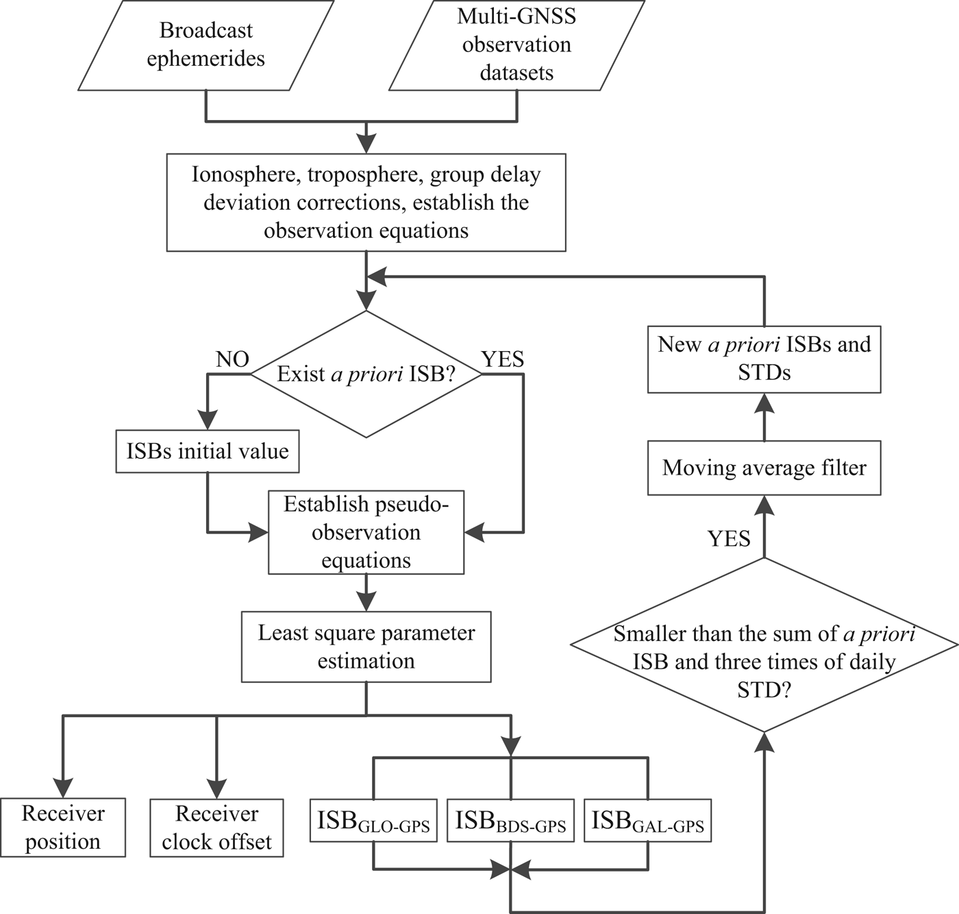
In the above observation model, the determination of the pseudo-observation B is vital. In the enhanced algorithm, it is determined by applying a moving average filter to smooth the ISB estimates at previous epochs, as depicted below.
 $$B(k) = {1 \over N} \sum_{i=k-1}^{k-N} ISB(i)$$
where B(k) represents the pseudo-observation B at the kth epoch, N is the moving window size. If the estimated ISB at the current epoch is smaller than the sum of the pseudo-observation B and three times its daily STD, the currently estimated ISB is input into the moving average filter to obtain an updated B for use in the next epoch. Otherwise, it is discarded. This smoothing procedure can control the quality of the pseudo-observation B especially when the number of satellites is insufficient at a certain epoch. For the first epoch, the earlier ISB estimate does not exist and thus the system time difference derived from the broadcast ephemeris is used as its initial value. In the case that the system time difference information is lacking in the broadcast ephemeris, the pseudo-observation B is initiated as zero but simultaneously a very small weight is assigned to the pseudo-observation. In addition, there is an end effect for the moving average filter during the first few epochs. To solve this issue, the mean value of the epoch-wise ISB estimates is used as its filtered value. In Equation (3), the pseudo-observation weight is determined by the variance of B. Figure 4 shows the flow chart of the enhanced multi-GNSS navigation algorithm.
Flow chart of enhanced multi-GNSS navigation algorithm.

4. ALGORITHM TEST IN DIFFERENT VISIBILITY CONDITIONS
Datasets in different satellite visibility environments are used to test the enhanced multi-GNSS navigation algorithm. In the implementation of the moving average filter, the smoothing window size is empirically set to five epochs. The enhanced multi-GNSS navigation algorithm is compared with the traditional multi-GNSS algorithm in which the ISBs are estimated as unknown parameters without utilising their a priori information. The unknown parameters are estimated on a single-epoch basis in both static and kinematic receiver tests.
4.1. Static Receiver Test
A quad-constellation observation dataset at a sampling interval of 30 s, collected on 1 August 2016 at GMSD, is utilised for the algorithm test. This GMSD station is chosen because more BeiDou satellites are visible at this station due to its low latitude. In order to evaluate the performance of the enhanced navigation algorithm, tests were carried out in three different satellite visibility conditions, namely open sky environment, blocked sky environment and critically blocked sky environment. For the open-sky environment, the satellite cut-off elevation angle is set to 15°, while the cut-off elevation angle is set to 50° to simulate the limited satellite visibility condition in the blocked sky environment. To simulate the critically blocked sky environment, only four different GNSS satellites as well as four GPS satellites are chosen in a criterion that their Position Dilution of Precision (PDOP) is analogous for comparison purposes. In the entire algorithm test, navigation solutions are output only when PDOP is smaller than 20. It should be noted that the multi-GNSS PDOP computation in the traditional algorithm is based on a design matrix with respect to three coordinate components, one receiver clock offset and three ISBs (Cai and Gao, Reference Cai and Gao2013) whereas the PDOP computation in the enhanced algorithm is only based on a design matrix with respect to three coordinate components and one receiver clock offset due to an inclusion of the ISB pseudo-observations, as with the standard PDOP calculation.
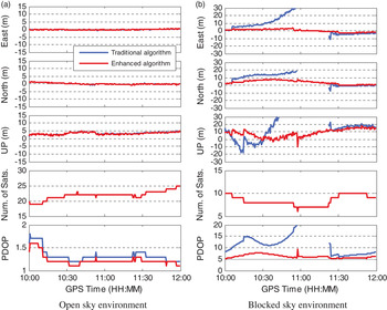
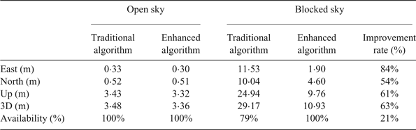
Figure 5 shows the epoch-wise position errors in three coordinate components under the open sky environment and the blocked sky environment, respectively. It can be seen that the enhanced algorithm can obtain the same position precision as the traditional algorithm under the open sky environment. However, under the blocked sky environment, the enhanced algorithm performs much better than the traditional algorithm. In particular, during the period 10:55 – 11:22, navigation solutions are not available using the traditional algorithm as the PDOP exceeds its threshold value of 20, whereas the navigation solutions are largely unaffected using the enhanced algorithm. The Root Mean Square (RMS) statistics of navigation solution errors are provided in Table 2. As more satellite observations are needed in the traditional algorithm, its performance decreases significantly when satellite visibility conditions worsen. Using the enhanced algorithm, the navigation solution accuracy is improved by 84%, 54% and 61% in the east, north and up components, respectively. The 3D position accuracy is improved by 63% and the availability of navigation solutions is improved 21% under the blocked sky environment.
Epoch-wise position errors using different navigation algorithms in the static receiver test.

RMS statistics of position errors under the open sky environment and blocked sky environment for static receiver tests.

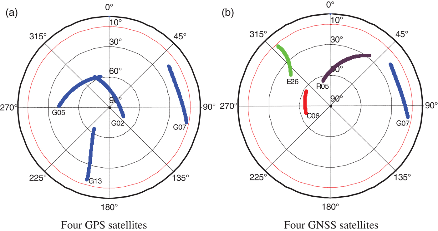
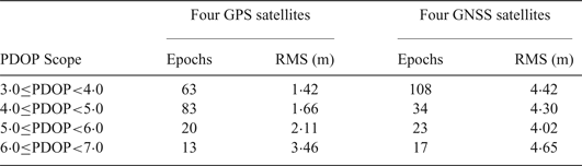
Under the critically blocked sky environment, sky plots of four GPS satellites and four different GNSS satellites at GMSD are shown in Figure 6, respectively. The a priori ISBs have been obtained when more than four GNSS satellites were available. RMS statistics are calculated based on the 3D position errors in different PDOP ranges using the enhanced navigation algorithm. Only the navigation solutions in the PDOP range of 3.0–7.0 are utilised for RMS calculation since most PDOP values lie in this scope from 10:00–12:00. The epoch number used and RMS statistical values are listed in Table 3. It should be noted that the statistical epoch number is different for four GPS and GNSS satellites when the RMS values are compared with each other. The enhanced algorithm with four GNSS satellites can obtain a navigation solution although its accuracy is degraded when compared with four GPS satellites. In contrast, navigation solutions are not available at all using the traditional algorithm with four GNSS satellites from different constellations.
Sky plots of four GPS satellites and four GNSS satellites at GMSD from GPS time 10:00 to 12:00.

RMS statistics of 3D position errors under a critically blocked sky environment.

4.2. Kinematic Receiver Test
A kinematic test was conducted on 16 August 2014 on the Central South University campus in Changsha, China. At the rover station, a “Trimble NetR9” receiver with a “Trimble Zephyr Model 2” antenna was carried by an electric bicycle. At the base station, the same type of receiver with a “Trimble Zephyr Geodetic 2” antenna was set up on a building roof about 2 km away from the rover station to help determine the reference coordinates of the rover station. The double-difference real time kinematic approach was applied to obtain centimetre-level accuracy for the rover station. Observations at a sampling rate of 1 s were collected from four GNSS constellations at a satellite cut-off elevation angle of 15°. The moving speed of the electric bicycle was about 10 km/h. The enhanced algorithm was tested under different satellite visibility conditions and compared to the traditional algorithm. In order to simulate a blocked environment such as in urban areas, 17 satellites are randomly excluded from all visible satellites in each 30 s.
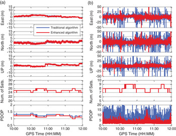
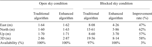
Figure 7 shows the position errors using two different navigation algorithms under open sky and simulated blocked sky environments in the kinematic test. As seen from Figure 7(a), the achieved performances using the two algorithms are similar, but in Figure 7(b), the enhanced algorithm significantly reduces the position errors. In addition, the PDOPs are lower using the enhanced algorithm, which explains why the position accuracy can be improved. Table 4 lists the RMS statistics of position errors under open sky and blocked sky environments using the traditional and enhanced navigation algorithm, respectively. Results indicate that the position accuracy is almost the same for the two different algorithms in the open sky condition, but in the simulated blocked environment, the improvement rates for the enhanced algorithm reach 47%, 62% and 57% over the traditional algorithm in the east, north and up components, respectively. The 3D position accuracy is improved by 58%. Of the navigation solutions, 3% are unavailable when the traditional algorithm is used whereas this is not the case for the enhanced algorithm. The availability is dependent on the PDOP and the number of visible satellites. When the PDOP exceeds its threshold value of 20 or the number of satellites is less than the required minimum number, the navigation solutions are considered unavailable.
Epoch-wise position errors using different navigation algorithms in the kinematic receiver test.

RMS statistics of position errors using different navigation algorithms in the kinematic test.

5. CONCLUSIONS
The ISB temporal variation characteristics between GPS and other GNSS systems are investigated. ISBs are estimated using datasets spanning about three years at five stations. The results indicate that the GLONASS-GPS, BDS-GPS and Galileo-GPS ISBs are stable in the short term with standard deviations of less than 5 ns but there are systematic varying trends over the long term for the GLONASS-GPS ISBs.
In light of the fact that the traditional multi-GNSS navigation algorithms sacrifice part of their observations in order to estimate the ISBs, an enhanced navigation algorithm is proposed by utilising the a priori information of the ISB. The enhanced algorithm is evaluated under open sky and blocked sky environments with a comparison to the traditional algorithm. The results indicate that the enhanced algorithm can achieve a similar performance under the open sky condition whereas much better performance can be achieved under the blocked sky condition with an improvement rate of up to 63% and 21% for 3D position accuracy and availability, respectively. Even for the case of four different GNSS satellites, the enhanced algorithm can still obtain a navigation solution. It is worth noting that the datasets used in this study were collected by geodetic-type receivers and the achieved accuracy is probably optimistic for navigation users who use low-cost receivers.
ACKNOWLEDGMENTS
The financial support from National Key R&D Program of China (No. 2016YFB0501803) and National Natural Science Foundation of China (No. 41674039) are greatly appreciated. Data contribution from IGS is also appreciated.