The Diffusion of Tractor Technology

DINAH DUFFY MARTINI; EUGENE SILBERBERG

doi:10.1017/S0022050706000155

The Diffusion of Tractor Technology

Published online by Cambridge University Press: 27 June 2006

DINAH DUFFY MARTINI and

EUGENE SILBERBERG

Show author details

DINAH DUFFY MARTINI: Affiliation:
Completed her Ph.D. at the University of Washington, Seattle.
EUGENE SILBERBERG: Affiliation:
Professor, Department of Economics, Box 353330, University of Washington, Seattle, WA 98195-3330.

Article contents

Abstract
THE MODEL
THE EMPIRICAL MODELS
RESULTS
CONCLUSIONS
Appendix: The Technical Coefficients—An OverviewDetails of these calculations are available from the authors. They are published in Dinah Duffy Martini's Ph.D. dissertation, “Technological Change in U.S. Agriculture: The Case of Substitution of Gasoline Tractor Power for Horse Power,” University of Washington, Seattle Washington, 2003.
References

Rights & Permissions

Abstract

A substantial literature exists claiming the adoption of tractors was inefficiently slow. We develop a linear programming model of farms that specifically incorporates the opportunity cost of the farmer's time and apply it to farms in Iowa during the interwar period. We develop technological coefficients derived at the task level, based on the data and agricultural reports from that period. By valuing the time saved by tractors, we demonstrate that the seemingly slow rate of tractor adoption was in fact wealth maximizing. Tractors were widely adopted only after the improvement in implements that came late in this period.

Information

Type: ARTICLES
Information: The Journal of Economic History , Volume 66 , Issue 2 , June 2006, pp. 354 - 389
DOI: https://doi.org/10.1017/S0022050706000155 [Opens in a new window]
Copyright: © 2006 The Economic History Association

For much of the last generation, economists have been saying that the adoption of the tractor was “too slow.” We contend that this perception is in part the result of an incorrect application of Paul David's 1966 threshold model. That model plausibly assumes that producers will switch to the most efficient (least cost) technology for accomplishing a task or set of tasks. Previous studies have focused on only one part of farming—raising crops. In this article we develop a model that incorporates the opportunity cost of the farmer's time and we apply the model to farmers in Iowa in the interwar period, a time when tractors came to resemble the machines we now recognize by that name. That is, we model the tractor adoption decision not as a horses or tractor decision, but rather as a horse farming versus horse and tractor farming decision. We show that an important reason why farmers switched to tractors was because they provided farmers with more time for noncrop activities, such as raising livestock, improving the farm infrastructure, or working off the farm. In fact it is more accurate to say that the tractor, by freeing up a farm owner's time to raise livestock or work off the farm, increased the opportunity cost of growing crops. With these results, explanations such as market imperfections and “lumpiness” of the inputs are not needed. The imperfect capital market explanation seems particularly suspect: farmers in fact bought cars, a purchase of comparable expense to tractors. In 1920, 74 percent of Iowa farms reported automobiles, even though only 13 percent reported tractors. In 1930, 85 percent of Iowa farms had cars, but only 27 percent had tractors.¹

McKibben and Griffin, “Changes,” table E-5, p. 106.

Among the first economists to apply the threshold model to tractors was Robert Ankli.²

Ankli, “Horses.”

Ankli concluded that the Corn Belt Farmers should have switched from horses to tractors above 46 acres and switched back to horses with more than 126 acres. When he compared the number of farms in this range with the number of tractors on farms, he concluded that the farmers had been slow to adopt. This is the genesis of the concept that tractors should have diffused faster than they did. Sally Clarke replicated Ankli's work for several combinations of horses and tractors.³

Clarke, “New Deal Regulation.”

She concluded that the threshold was 67 acres for teams of six horses and 61.4 crop acres for five horse teams. According to her research, 70 percent of farms should have benefited but only 30 percent had tractors. Clarke noticed that there were fewer tractors in the counties where the average cash margins were the lowest. From this she theorized that the cause of the low adoption rates in 1920s and 1930s had occurred because of farmer fears of bankruptcy and the low state of farmer bank accounts throughout the 1920s.

William White argues that Clarke's threshold acreage is actually too high.⁴

White, “Unsung Hero.”

From his work on a hedonic price index for tractors, he found that the initial cost of a tractor in 1929 was $875 instead of the $1,000 Clarke used. In his calculations with this lower initial cost, the threshold disappears completely. His conclusion is that everyone should have been farming with tractors. Byron Lew adds the element of uncertainty to the threshold model by introducing the role of agricultural prices and costs in this period and the uncertainty inherent in a rapidly evolving technology.⁵

Lew, “Diffusion.”

He first calculates the threshold at which farmers should rationally switch using several sizes of horse teams and horse and tractor combinations without uncertainty. He essentially finds the same result as the previous authors: the predictions of the threshold model do not match the data on Canadian prairie farms. He then explored the impact of uncertainty in input prices, output prices, and tractor evolution. He finds that as output prices trend downward, there is less likelihood a farmer will buy a tractor. However as the price of a tractor tends downward, he also does not buy. This last result seems odd, but he explains that as the tractor becomes more and more capable, the farmer is tempted to put off the buy decision because he could get a better one next year at the lower price. When Lew recalculates the threshold acreages accounting for the uncertainty, he finds that his model predicts adoption rates closer to the data than the thresholds of Ankli and Clarke.

Alan Olmstead and Paul Rhode develop a simultaneous equation model and apply it to state-level data to test the impact of the tractor on cropland acres per farm.⁶

Olmstead and Rhode, “Reshaping the Landscape.”

They find that farm scale and tractor adoption are co-determined, meaning in particular that crop acreage is not exogenous. They also argue that the rapid fall in the price of horses explains the slower adoption in the South, and also point out that the decline in horse prices was itself an endogenous result of tractor adoption. Although they stress the labor-saving aspect of tractors, Olmstead and Rhode do not formally model this important determinant of the adoption of this new technology.

In his classic 1960 article on tractor adoption, Zvi Griliches, using national data, found investment in tractors to be dependent on the price of crops.⁷

Griliches, “Demand.

Griliches's 1957 paper on the adoption of hybrid corn concluded that “Where the profits from this innovation were large and clear cut, the changeover was very rapid.”⁸

Griliches, “Hybrid Corn,” pp. 501–22.

We believe the shortcoming common to this previous research is that it investigates only the cost of growing crops. Although researchers have often mentioned that tractors saved time, this aspect of production has not been specifically incorporated into the models. The tractors did not necessarily result in the farmers having a larger corn crop; output was constrained by the land and the farm technology at the time. But farmers also generated income by raising livestock, improving the farm, and working off the farm. By saving time using a tractor, farmers could generate additional income through these other activities, or simply consume greater leisure.

Although we and others construct average costs and average technical coefficients of production, these are not necessarily any one farm's marginal costs or benefits. The marginal benefits of using some technology varied from farm to farm depending on the other inputs the owners had available, especially the farmer's human capital related to the use of horses. A 1935 farm study found that younger farmers were more likely to adopt tractors than their older colleagues.⁹

Hopkins, “Changing Technology,” p. 63.

This is what one would expect on the basis of elementary considerations of human capital theory—older farmers would likely be the ones whose skills with horses would be relatively greater, and younger farmers have a greater potential gain from incurring the costs of adopting new technology, because they will have more years to apply that technology. All we can say with data of this sort is that as the average benefits of tractors rises relative to horses, we expect the rate of switching from horses to tractors to increase.

We restrict our analysis to Iowa farms in the interwar period. National-level data obscure many important influences and variations in the diffusion of tractors. The diffusion of the tractor was not uniform across the United States. As the tractor developed, various farming systems found them useful, albeit in different decades. Very roughly, the small grain region and Far West were the earliest adopters. This farming system has an annual cycle of plow, plant, and reap. Although the planting was usually done with horses, plowing and reaping could be done with tractors. The huge power needs of these tasks made the tractor a valuable addition to the farm and reduced the number of horses needed. The more complicated farming system of the Corn Belt has a cycle of plow, plant, cultivate, and hand harvest for crops. Because of smaller acreages and cultivation between the rows of corn, tractors did not displace many horses until the introduction of the Farmall tractor in 1924.¹⁰

The Farmall was the first tractor with the modern set-up of two small front wheels close together and large rear wheels on a high axle. This permitted tractors to cultivate crops (turn over the soil, weed) until the crops reached the height of the rear axle.

Adoption in the eastern states was more individual as the evolution of the tractor and specific implements became available. Thus it is important to segregate the type of farming by region or even state. For this reason, and because of data availability, we restrict our analysis to farms in Iowa from 1920 to 1940.

THE MODEL

In order to investigate the incentives that farmers faced affecting the rate of substitution of tractors for horses, we need a tractable (no pun intended) model of farms that captures the changing costs and technology that led to this substitution. We analyze those incentives using a multi-year linear programming (LP) model. To capture the dynamic aspects of farming technology, we repeat LP models over the years 1922, 1930, 1936, and 1940. Each LP model generates a Lagrange multiplier (“shadow price”) for tractors and horses and a value of the objective function for each period. In this manner we can see how these net incomes and shadow prices change over time. We show that these values are consistent with the slow adoption of tractors in this period.

We posit that farmers maximize their net income by choosing the proper levels of corn, oats, and hay (x₁, x₂, x₃) with a fixed coefficient technology, using priced and unpriced inputs and fixed resources, subject to resource constraints. The technical coefficients, the a_ijs, are the amounts of input i necessary to produce one unit of output j. We define one unit of corn or oats to be 100 bushels; one unit of hay is one ton. We use the subscripts i (1,2,3,4) for the inputs land, man-hours, horse-hours, and tractor-hours, respectively, and j (1,2,3) for the outputs corn, oats, and hay, respectively. The farmer's net income is the income he receives from sale of the crops less the cost of the inputs used. Here, the priced inputs are horses and tractors only.

In our model we do not include labor as a priced input. It seems most likely that the farmers on 160 acre farms used family labor almost exclusively. Shaw reports that there were approximately three unpaid family workers for every hired worker in 1930.¹¹

Shaw et al., “Trends,” table H-2, p. 154.

(The Census definition of “family labor” was work done by family members without pay.) In 1930 there were, on average, 0.54 hired workers per farm.¹²

U.S. Bureau of the Census, “Fifteenth Census,” vol. 3, table 20, p. 789.

(The index of hired workers displayed in Table 1 implies there would have been slightly more hired workers in 1920, and fewer as the 1930s progressed.) Thus on average, the workers on a 160-acre farm were 1 farmer-operator, 0.54 hired workers, and an additional 3 × 0.54 = 1.62 unpaid family workers for a total of 3.16 individuals. The hired workers thus constituted only about one-sixth of the total workforce. Further, if one supposes that the distribution of hired labor was greater on the larger than average farms, then the farms modeled in this article were most likely run by family members. The inclusion of the relatively small hired labor input into the objective function would not likely change any of the results.

Denoting the unit prices of horse and tractor hours as w₃ and w₄ respectively, the cost of each input is the sum of the amounts of that input used in each crop times its respective input price. The net income the farmer receives is thus

The resource constraints simply state that the amount of each input used cannot exceed the total amounts of those inputs that are available, represented by the right-hand side coefficients:

This simple model, however, ignores important constraints the Iowa farmers faced. When this model is solved with actual data, it says that farmers would plant only corn on every available acre. In fact, farmers planted corn, oats, and hay in fairly persistent proportions year after year. This seemingly non-wealth-maximizing behavior has two explanations: land fertility considerations and the episodic nature of the labor requirements of corn.¹³

Hopkins, “Crop System,” p. 287, table vii. Thomas and Hopkins, “Seven Iowa Counties,” figure 3.

Thus, the basic model must be extended to include crop rotation and seasonality constraints.

Crop Rotation

Crop rotation was a way for farmers to keep their yields of corn high. Data from records kept by the Iowa Agricultural Experiment Station on fields that had been kept in corn for three or four years indicated that corn yields dropped by 12.3 percent in the second year, by 15.2 percent in the third year, and 32.7 percent in the fourth year.¹⁴

Hopkins, “Crop System,” table 7, p. 287.

These results are supported by a 30 year study reported in 1941. In that study, yields dropped 35 percent in four years.¹⁵

Chen and Arny, “Crop Rotation Studies,” p. 4.

It can easily be shown that failing to rotate crops eventually resulted in lower net incomes for the farmers.

With chemical fertilizers not generally available in this time period, farmers dealt with this loss of yield by rotating oats and hay with the corn. The typical rotation was to divide the farm into four sections, and grow corn in sections 1 and 2, oats in 3, and hay in 4. The next year the farmer would grow the same crops but start with section 2, and so on. Thus, although the crop rotation process is a chronologically sequential one for a particular farm, the proportions of land on the farm in various crops remained the same. Although a more complete, multiyear model would generate this crop rotation as part of the solution, we simplify the model by requiring the farm to have the same acres in oats and hay as did the average farm for that year. Because the solution will always fill all available land with corn production, constraining the number of oat and hay acres is all that is needed.

The Crop Rotation Constraints are thus:

Seasonality

Although the farmer had approximately 3,120 work hours per person available to him (10 hours per day × 6 days per week × 52 weeks), bad weather, the uneven distribution of labor requirements throughout the year, and the physical limit to a work day of 10–12 hours meant that at no time did the farmer have all of his annual labor available to him. Labor hours become very constraining at the times of the year during spring planting and fall harvesting. Of these two, the spring planting time was the most demanding because there was a narrow window of opportunity to get the crops planted. According to H. L. Thomas and John A. Hopkins, doing the needed work at just the right time seems to be one of the most important influences in obtaining a satisfactory yield at the least cost.¹⁶

Thomas and Hopkins, “Seven Iowa Counties,” pp. 23–24.

Farmers generally plan to do the seedbed preparation and planting in the first two weeks in May.¹⁷

Richey, “What and How of Hybrid Corn,” p. 17

In a 1922 study (published in 1926), George Pond found that farmers in southwestern Minnesota (just north of the cash grain area of Iowa) began plowing in mid-April and planted until late May.¹⁸

Pond, “Study,” p. 44.

Pond found that on average, after allowing for weekends and rainy days, there were 21 days available for spring plowing and planting.

In the fall the crop must be harvested as soon as it is ripe so that an early winter does not prevent the crop from being harvested. Once there is snow on the ground the horses and machines cannot get into the fields to harvest.

We capture the intertemporal nonsubstitutability of labor by dividing the year into three important windows of time and matching the labor available to the power needs for each set of tasks. Because the amount of labor used for plowing cannot be substituted for the harvesting of grain and there are definite dates between which specific tasks must be performed, for each crop we calculate three season-specific technical coefficients for each labor constraint, each horse hour constraint, and each tractor constraint. Only one technical coefficient per crop is needed for the land because land is allocated only once a year.

The seasons are: Winter: This is the month of April when the oats can be planted. The oats germinate in colder wetter soil than corn so they can be planted even when there is still a threat of frost. Spring: This is the corn seedbed preparation and planting period. This period is bounded by the last day of frost and June 1. As mentioned, the farmers planned about 21 workdays to accomplish the preparation and planting on the number of acres designated for corn. Summer & Fall: This is the period from June 1 through the end of harvest. The tasks done are cultivating the corn in June and July, harvesting the oats in July and harvesting the corn from late September on.

We add a third subscript k(1,2,3) to indicate the season. For example, a₂₂₃ is the technical coefficient for the man-hours used for oats in the Summer & Fall. Note that

, i = 1,2,3,4, and j = 1,2,3.

The Opportunity Cost of Labor

As we have stressed, the major benefit of using tractors was that the labor input dropped dramatically. If the farmer spent less time raising crops he would have more time for noncrop activities such as raising livestock, improving the farm infrastructure, or working off the farm. There is an implicit cost of the farmer's labor that must be considered. We have modeled this opportunity cost of the farmer's time by modifying the objective function.

Let

be the endowment of all the hours the farmer has available to him, and let w₂ represent the opportunity cost of this labor. Recall that a₂₁, a₂₂ and a₂₃ represent the labor hours summed over all seasons for raising a unit of each crop. Then the amount of time the farmer has to work in activities other than crops is

Multiplying this quantity by the alternative wage represents foregone earnings in livestock, infrastructure improvements, or off-farm employment.

The final model in its entirety is thus:

subject to resource, seasonality, crop rotation, and non-negativity constraints:

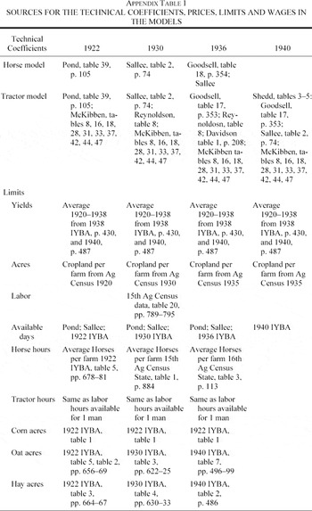
All parameters were derived from reports in the literature of the time. The technological coefficients were derived at the task level, as indicated in the Appendix. The principal sources were the Agricultural Experiment Station (AES) Reports of Iowa, Minnesota, and Illinois, Iowa Year Book of Agriculture (IYBA) for each year, and the various publications (Farmer's Bulletins, Department Bulletins, Miscellaneous Publications and Technical Bulletins) of the United States Department of Agriculture (USDA). Specific citations are available from the authors upon request.

Structural Stability, 1920–1940

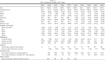
We assume throughout that yields (bushels per acre), farm size, price, and wages were constant. By 1940, 55 percent of the farms had tractors, but the manner or scale of farming had not changed, as the data in Table 1 clearly show. Farm size varied by only 3.3 acres over the period, corn acres fluctuated between 104.72 in 1930 to 90.28 in 1935 but over the period remained virtually flat. The same agronomic techniques prevailed—the crop rotation system and the numbers of times operations were performed remained unchanged, and the yields per acre all remained constant.

Although the period of study is 1920 to 1940, Table 1 covers 1910–1960 so that the period of study can be seen within the longer-term trends. Comparing across the columns one can see that the farm size changed little over the first four decades of the twentieth century. After 1940 the size begins to climb and by the 1960s the average farm size was almost 200 acres. The proportion of acres in corn oats and hay vary slightly, but with no discernible trend between 1920 and 1940; the proportion allocated to corn begins to rise through the 1950s. Although the number of horses declined by almost 50 percent over the period, the proportion of oats, usually considered to have been grown for horse feed, surprisingly did not change, and pasture acres increased 13 percent. The data on livestock are ambiguous: The number of beef remains flat but the dairy cows rise during the period. Of note, however, is the increase in the number of cattle marketed and the number of gallons of milk sold. The increase in marketing quantities suggests the farmers were spending more time and assets in livestock operations. Hogs decline during the period of study but not over the longer haul. This hog decline was due in part from the policies of the New Deal but swine cholera was also a major problem of the day. Finally, the number of sheep on farms fluctuates but the amount of wool produced rises.

A very interesting and important indicator for the purposes of this study is the rising trend of farmers working more than 100 days off their farms and the steady decline in the index of average number of hired workers. The most important effect of tractor technology was to reduce the labor input required for field crops. The upward trend of work off-farm illustrates one of the ways that farmers used the hours released from farming to increase their total annual income.

Isolating the Effects of Technical Change

Tractors improved throughout the interwar period. The Fordson tractor in 1918 could plow but not cultivate, and it had a tendency to flip backwards onto the operator when it hit obstructions or very soft ground. The Farmall in 1924 was the first tractor that could cultivate young corn plants. Over the next 15 years, manufacturers developed better metal alloys and tractor designs. Other developments included an expanding array of specialized implements culminating with Harry Ferguson's three point hitch in 1939, hydraulics for lifting implements, and rubber tires. Only with the advent of the Ford Ferguson 9N circa 1940 were all of the basic elements of modern tractors introduced.

Exogenous effects such as variations in weather can obscure these technological changes. For example, if yields are low because of weather, the a_ijks for the inputs will be higher, obscuring the advances in tractor design that would lower the a_ijks. Removing these exogenous effects is critical to drawing accurate conclusions from the results. We therefore apply the model to each observation period as if the same farmer worked the same farm using the same farming method with horses or with horses and a tractor at each observation point. In this case, because we are interested in the effects of technological change, we hold the yields, farm size, prices, and alternative wages constant.¹⁹

There is a slight upward trend in corn and hay yields due to the introduction of hybrid corn and alfalfa hay in the last years of the period. Oat production remained flat.

We have used the average yields for the period 1920–1938.

In addition to weather, there are three other important exogenous effects at work that can affect the implicit prices of tractors and horses from one year to the next: the evolution of agriculture towards greater efficiency in the use of the inputs (learning effects), severe macroeconomic shocks to the economy, and scale effects. Throughout the two decades of our study, the Iowa Agricultural Experiment Station (and others like it) conducted studies and promoted greater efficiency in farming, in terms of, for example, the number of times various tasks had to be done. This secular growth in knowledge is largely a separate issue from the choice of tractors vs. horses, and so in this study we use the same set of tasks for each period.

During this period, there were some important macroeconomic shocks, one of which was the drop in real agricultural wages in the 1930s.²⁰

See U.S. Bureau of the Census, Historical Statistics, especially Series E 113–139, pp. 125–26, Consumer Price Indexes (BLS) by Major Groups and Subgroups: 1890 to 1957, Series K 73–82, p. 280; Farm Employment, Wages, and Man-Hours Used for Farmwork: 1866–1957; Series D 626–634, p. 92, Hours and Earnings for Production Workers in Manufacturing: 1900 to 1957. It is clear that nominal farm and manufacturing wages fell, but real farm wages fell absolutely, whereas real manufacturing wages remained steady from 1929 through 1933 and then rose slightly for the rest of the 1930s.

We discuss wages further below, in particular, the role wages played in determining the opportunity cost of the farmer's labor as a farmer. A drop in the real agricultural wage in the 1930s would tend to reduce the incentives for adopting labor-saving devices such as tractors. We capture this effect by using an alternative wage ranging from zero to $0.55 per hour.

Lastly, we ignore the minor effects of economies of scale in this period in our model. In fact farm size changed very little over the period as Table 1 shows. The crop acres average 100.13 and so 100 acres has been used in all the models as the land limit. We use the actual average acres of oats and hay in each period.

THE EMPIRICAL MODELS

Linear programming models generate positive shadow values only for those constraints that are binding.²¹

The number of binding constraints cannot exceed the number of decision variables, in this case, three. (See, for example, Silberberg and Suen, Structure, especially section 17.2 & ff.) If a constraint is binding, it is easy to calculate the increase in the objective function value (net income) that would occur if, say, one more acre of land were available. This increase in income represents the value of the marginal product (VMP) of land, and thus the implied competitive price of this resource. If a constraint is not binding, meaning there is an excess of the resource over what the solution requires, then the VMP, or shadow price of that resource is zero, even though its average value is obviously not zero. These “shadow prices” or “Lagrange multipliers” are generated as part of the solution.

For the Iowa farmers in this study, the land limit was the overriding constraint. Those farmers assembled the inputs that allowed them to plant as much land as was available. A second binding constraint is the oats crop rotation constraint. This constraint is used to model the reality that corn could not be planted year after year on the same land without severe losses in yield. Requiring that the solution include the number of oat acres planted in each observation year provides a simple way to account for deteriorating corn yields over time from repeated planting. The shadow value of an acre of oats is always negative because in these static models (ignoring the benefits of crop rotation), diverting acreage from corn to oats lowers net income.

When the models are run, the tractor and horse-hours constraints turn out to be nonbinding, producing zero shadow prices. The number of hours theoretically available for tractor and horse-hours does not adequately reflect the peak time constraints the farmers faced. We therefore parametrically reduce the Spring right-hand side time limits for horse and tractor-hours until these constraints became just binding. That is, after the model determines how many Spring horse or tractor hours the solution requires, we reset the horse or tractor constraint to that level. This procedure allows the model to generate positive shadow values for these resources without changing the solution, so that a comparison of the marginal productivities of these two power sources becomes possible.

It is a fair criticism of the model that—because there can be only three binding constraints, one of which is obviously the land constraint, and the two others turn out to be the crop rotation constraints for oats and hay (until we parametrically lower the Spring power source constraint until it becomes just binding, replacing the crop rotation constraint for hay)—the solution is in a real sense pre-ordained to have the farmer plant approximately half of his acreage in corn, and approximately 25 percent in oats and the remainder in hay. These elementary predictions of the model in fact accord with reality—this is what these farmers actually planted, with only very small deviations, every year (see Table 1). Though the model is framed to derive the optimal crop mix, this is not its real purpose—Iowa farmers in the interwar period had very little choice about this due to the necessity for crop rotation. Rather, our purpose is to derive the shadow prices of the two alternative power sources, to see how changing technology affected their relative prices and farm income, and to investigate the role of the opportunity cost of labor. Moreover, once the model determines which three constraints are binding, we can analyze the technical coefficients of those constraints to gain a better understanding of exactly what is driving the results.

We run several comparative statics experiments using various hourly real wages the farmer might have had in 1910–1914 dollars to examine the incentive farmers had to switch to tractors: zero alternative wage, an average farm wage, and the average manufacturing wage (w = 0, $0.27, $0.55 per hour, respectively). We assume the annual time available to farmers is

= 3,120 hours (10 hours per day × 6 days per week × 52 weeks). However, the seasonal constraints are narrow windows of opportunity, and we use the reduced number of hours available for each season in those constraints. We use a wage of $0 to model the polar case where the farmer had no alternative use for his time. This is the assumption most previous authors have implicitly or explicitly used.

²²

This would imply that farmers valued their leisure at zero; we do not intend to imply that this is a true reflection of their time value. We simply use this to illustrate the effects of ignoring the farmer's value of time saved.

We use the average farm wage of $0.27 to model the effect on the farmer's incentives of using his nonfield crop time to work for another farm, farm more acres himself, or spend more time on livestock. One of the reported changes that occurred when farmers got tractors was that they did custom work for their neighbors. Because the work they did replaced other hired labor, the average farm wage without board is a reasonable and plausible proxy. The manufacturing wage of $0.55 models the wage available to farmers who found off-farm work in nonagricultural occupations. We use the manufacturing wage because in 1935 nonagricultural occupations were reported for three-fourths of the off-farm days.

The real horse-hour cost varied from $0.09 to $0.10 for all the observation periods, while the real tractor cost varied from $0.54 in 1922, to $0.37 in 1930, and $0.41 in 1936.²³

Tolley and Reynoldson, “Cost”; Reynoldson et al., “Utilization”; and Goodsell, “Cost.”

(There was no report in 1940 because only tractors were used. We used the 1936 horse farming data for 1940 horse farming. We incorporated the mechanical corn picker in the technical coefficient for corn harvesting in 1940 on tractor farms. These are averages obtained from surveys of men who had used tractors for at least one season. There are large variations in the reported hourly costs for both horse and tractors. The number of hours the power source was used varied widely with farm size as depreciation was the greatest proportion of cost. Because the 100-crop-acre farm was the most common size, using these averages is the most appropriate. The prices received for feed grains were used to deflate the costs into 1920–1914 = 100 values. The tractor costs were deflated by the “Prices Paid Index for all Commodities used in Production by Farmers.”²⁴

U.S. Department of Agriculture, Major Statistical Series, p. 17. These hourly costs are calculated as follows: First the initial cost of the horse or tractor depreciated over its life, then costs for feed, bedding, veterinary fees and a 5 percent interest on the capital investment area added in the case of the horse. For the tractor fuel, oil, grease, repairs, and a 5 percent interest on the capital investment are added to the depreciation for each year. These total are then divided by the number of hours each are used annually. The result is the hourly cost for using the power source. In previous studies, the authors calculated the costs in the same manner.

In order to isolate the effects of technological change, we hold the costs constant in all the models that follow. We use costs of $0.09/horse hour and $0.50 per tractor hour. Because the tractor hour cost declined, the shadow values for tractors are understated, but, again, holding the costs constant has the advantage of isolating the effects of technological change.

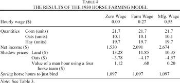
The following pages contain the actual models we ran, with land, yields, farms size prices, and wages held constant. The objective functions and constraints are presented with their numerical coefficients, followed by the LP results. For each time period we run a horse farming model and a tractor-farming model. In the horse farming models we assume that horse teams powered all the tasks throughout the year. In the tractor-farming models, the distribution of tasks varies with the capabilities of the tractors over time. For example, in 1922 tractors only did the seedbed preparation tasks, but by 1940 they were used for all the tasks.

In all the models that follow, the technical coefficients over time decrease for both types of farming. For example, in 1922 it took 51.44 man hours to grow and harvest 100 bushels of corn with horses; in 1930 it took 35.41. With tractors it took 48.06 man-hours in 1922 and 28.78 in 1930. As a result, the number of men and horses required to grow the corn and other crops steadily decreases throughout the period of this study, and indeed, throughout the rest of the century.

The technical coefficients were all derived independently of each other and independently of the resource constraints. Each crop was divided into the tasks that needed to be done to grow and harvest each crop. Then the Agricultural Experiment Station and USDA reports for the length of time each of these tasks took per acre were used to separate the tasks into their appropriate season and to derive the total hours necessary in man, horse, and tractor hours to produce each crop. The resource limits were taken from census data on the resources available. The crop acreages turn out to be the limiting resources. Men, horse, and tractor hours available are in each case greater than the resources necessary to produce the optimum quantities. The Appendix contains citations for these sources.

1922 Horse Farming Model

subject to resource, seasonality, crop rotation, and non-negativity constraints:

where p_i = (59,31,10), x_i = (x₁, x₂, x₃), w₂ = $0, $0.27, $0.55, w₃ = $0.09

1922 Tractor Farming Model

subject to resource, seasonality, crop rotation, and non-negativity constraints:

where p_i = (59,31,10), x_i = (x₁, x₂, x₃), w₂ = $0, $0.27, $0.55, w₃ = $0.09, and w₄ = $0.45

1930 Horse Farming Model

subject to resource, seasonality, crop rotation, and non-negativity constraints:

where p_i = (59,31,10), x_i = (x₁, x₂, x₃), w₂ = $0, $0.27, $0.55, and w₃ = $0.09

1930 Tractor Farming Model

subject to resource, seasonality, crop rotation, and non-negativity constraints:

where p_i = (59,31,10), x_i = (x₁, x₂, x₃), w₂ = $0, $0.27, $0.55, w₃ = $0.09, and w₄ = $0.45

1936 Horse Farming Model

subject to resource, seasonality, crop rotation, and non-negativity constraints:

where p_i = (59,31,10), x_i = (x₁, x₂, x₃), w₂ = $0 $0.27, $0.55, and w₃ = $0.09

1936 Tractor Farming Model

subject to resource, seasonality, crop rotation, and non-negativity constraints:

where p_i = (59,31,10), x_i = (x₁, x₂, x₃), w₂ = $0, $0.27, $0.55, w₃ = $0.09, and w₄ = $0.45

1940 Tractor Farming Model

subject to resource, seasonality, crop rotation and non-negativity constraints:

where p_i = (59,31,10), x_i = (x₁, x₂, x₃), w₂ = $0, $0.27, $0.55, w₃ = $0.09, and w₄ = $0.45

RESULTS

It is important to understand that it is improving technology that drives the results that follow. In all the models, it turns out that the three constraints that determine the solution are the land constraint and the oats and hay crop rotation constraints. When we reduce the spring power constraint so that it becomes just binding, that constraint replaces the crop rotation constraint for hay. Since the oats crop rotation constraint alone determines the output of oats (which changes little over this period), and the land resource constraint is unchanged in all the models, it is, first, the reduction over time of the technical coefficient for the spring power constraint (a₃₁₂ for horse farms and a₄₁₂ for tractor farms), and second, the decrease in the technical coefficients for the over-all man-hours constraint, that produces the changes in shadow values and net incomes that are of interest. For horse farms, the amount of horse-hours needed for planting the acreage to produce 100 bushels of corn falls from 61.67 in 1922, to 50.63 in 1930 and to 44.73 in 1936. For tractor farms, the number of tractor hours needed to plant acreage for 100 bushels of corn falls from 8.63 in 1922 to 6.35 in 1930, to 5.51 in 1936 and to 4.93 in 1940. This is a reduction of 27.5 percent for horse farms and a 37.2 percent reduction for tractor farms between 1922 and 1936, and a 43.9 percent decrease for tractor farms by 1940. Thus there was technological progress for both horse and tractor farms, but the pace of progress was faster for the farms that used tractors. Similarly, on farms using just horses, it took 51.44 man-hours to produce 100 bushels of corn in 1922, and 31.10 man-hours in 1936. By contrast, using tractors, it took 48.06 man-hours to produce 100 bushels of corn in 1922; in 1940, it took only 12.51 hours, an almost four-fold reduction. These reductions came in part from the continuing evolution in tractor design and in the metallurgical advances applied to implements for both methods of farming. For example, the speed of horse farming improved when more efficient implement designs were made with harder and stronger materials. In tractor farming, as the power and versatility improved, more ground could be covered in shorter times.

We now present and analyze the results of these models.

Zero Alternative Wage Value

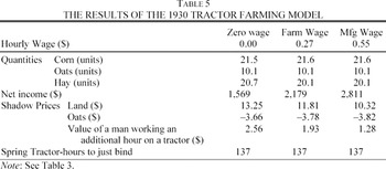
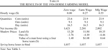
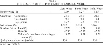
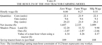
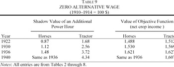
The Zero Alternative Wage experiment produces the shadow values and maximum net income values shown in Table 9. In this table and the ones following, “Horses” refers to a four-horse team, the most common team size in this period.

In every observation year the amount of revenue one man can generate by driving an additional tractor hour is absolutely higher than the value he can produce when driving a horse team for an hour. Additionally, the spread between these shadow values widens over time. The 1922 shadow value of tractor-hours is 93 percent higher than the shadow value of a horse team hour; in 1930 it is 129 percent higher; in 1936 it is 151 percent higher and in 1940 it is 193 percent higher. These are the results that have led previous authors to conclude that if farmers were wealth-maximizers they should have begun adopting tractors in great numbers in the 1920s unless some market imperfection caused delays.

However if farmers made their decisions to substitute technologies based on the total crop income alone, as previous authors implicitly assume, the very small variations in net income found in Table 9 clearly suggest that from the perspective of his annual income, a farmer in fact had little incentive to change. Technological improvements in implements for horse farming allowed farmers to reduce the number of horses used. As late as 1936, the crop income from horse farming was comparable to tractor farming, indicating little incentive to change technologies. As long as a farmer worked with his horses until all the crop acres were planted, he could produce the same level of corn, oats, and hay on the same number of acres, i.e., the same gross crop income, with horses as he could with tractors. There was little incentive to make the outlays for a tractor and take on the uncertainties of a new technology because the hourly cost of the two technologies was quite close.

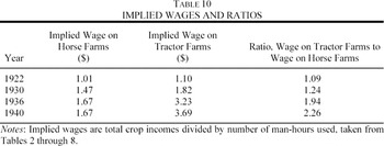
Dividing the total crop income by the number of man-hours used produces the implied average time values of farming crops in these years shown in Table 10.²⁵

We are indebted to an anonymous referee for suggesting these calculations.

Note that the internal wage rate for raising crops increases over time for both horse and tractor farms, but that the ratio of tractor to horse farm wages increases substantially over time. The reason for the increase in this ratio is mainly the substantially greater reduction in hours required to produce all the crops the land could bear when the farmer used tractors versus horses. We can presume the farmer valued these hours saved, either for leisure or for the ability to earn additional income in some other activity. Thus the time saved is an important component of the reason for the switch to tractors. The size of these internal wages are in fact substantially greater than what we find (55 cents) in the manufacturing sector. This would provide an incentive to expand the farm acreage and raise additional livestock. It also should have resulted in increased rents on the specific factor, land, in this period. However we see little of these effects in the interwar period: farm size and livestock levels remained stable, and work off the farm increased only slightly between 1930 and 1940. (Off-farm work may have increased from 1922, but we are not aware of any data for this.) Livestock levels may have remained constant in this period because even with tractors, corn output, used mostly for feed, did not increase.

It is not clear, however, that the farmer had available to him time that had this value at the margin. Without changing the size of the farm, at the margin, the farmer's alternative wage was the greater of the value of his leisure or what he could earn with various chores, i.e., improving the existing capital on the farm, producing livestock, or working off the farm. As we have noted, the technological improvements that occurred in the interwar period did not result in higher crop levels—it just took farmers less time to produce the crops. With the same output of corn (mostly used for feed), there was little added incentive to raise additional livestock. It was only after World War II that these effects become evident in the data, and this is when further innovations, particularly the use of fertilizer, hybrid corn, and soybeans (which were nitrogen fixing and thus reduced the need for crop rotation) do farm sizes and livestock levels increase. Thus, the relevant wage to evaluate the farmer's time should be the farm and manufacturing wages we consider.

We now demonstrate how allowing for a positive alternative wage for farmers resolves some of the mystery regarding the slow pace of tractor adoption.

Average Iowa Farm Wage

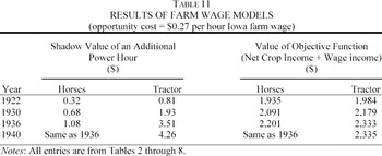
The effect on the shadow values of tractor and horse-hours when there is an alternative use for the farmer's time is shown in Table 11, which utilizes a farm wage of $0.27 per hour for the opportunity cost of the farmer's time.²⁶

U.S. Department of Agriculture, Major Statistical Series, p. 17, table 28, page 80.

The per-hour horse cost and tractor cost are held constant in this experiment.

Again we see the same pattern. As with the zero alternative wage experiment, we see that the absolute shadow values are higher for a tractor hour than a horse team hour but the relative value between the two widens over time at a faster rate: $0.75/$0.32 = 2.34 in 1922, rising to $4.26/$1.08 = 3.94 in 1940.

More interesting is the relationship of the maximum net income levels. The objective function is the sum of the net value of the field crops and the wages a farmer could earn with the hours of his endowment beyond those needed for the crops. At $0.27 per hour there is a $49 difference between the maximum net income for horse farming or tractor farming in 1922 but in 1936 there is a $132 difference.²⁷

We also ran the model with the actual reported costs of tractor and horse-hours stated above; that model produced an increase in net income of $109.

Henry Ford lowered the price of his Fordson tractor to $395 in the mid 1920s in his marketing war with International Harvester.²⁸

Williams. Fordson, p. 55.

Used tractors could probably be purchased for approximately $200, so in 1936 a farmer might be enticed to give tractor farming a try. These results more accurately reflect the observation that farmers valued the time saved. For example, Hopkins cites the improvement in farms through installation of drainage tiles during the 1930s and from more modern husbandry practices.²⁹

Hopkins, “Changing Technology,” p. 37.

This wealth-enhancing activity became more feasible as the time used to raise crops decreased. By using their time saved to add to their income from other sources, farmers enhanced their returns on capital.

Note especially how a positive alternative wage causes a larger effect on net income. Rodolfo Manuelli and Ananth Seshadri concluded that the rising manufacturing wage led farmers to adopt tractors because that rise made farm labor more expensive.³⁰

Manuelli and Seshadri. “Frictionless Technology Diffusion,” pp. 24 and 27.

However, the major switch to tractors took place during the 1930s, when real wages declined. As the alternative wage rises, the shadow value of a tractor hour rises faster than the shadow value of horses. This suggests that the farmer would have bought a tractor so that he could capture the high manufacturing wage for himself, i.e., that it was the opportunity cost of the farmer's own time that caused the switch.

A somewhat surprising result in this experiment is that the absolute values of horse and tractor hours decline when a positive wage is used and wages rise. This happens because the endowment of man-hours is fixed at 3,120 hours. The farmer can either raise crops or do some other work. Every hour he works on crops is one fewer hour he can work elsewhere. The farmer will earn the income from the crops grown, but will lose the income he would have earned but for the extra hour he put into crops. Thus, as the alternative wage rises, the net marginal value of additional inputs into farming declines.

A second unexpected result is the large increase in the shadow values for horses. Throughout the observation period, horse implements got bigger and stronger, partly from some spillover from the work being done on tractors and their implements, and partly the from continuation of the remarkable horse farming innovations, such as the reaper, that had already brought agriculture to a higher level of productivity. This provides an additional reason why the switch to tractors took place slowly over two decades.

The Average U.S. Manufacturing Wage

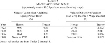
The next experiment uses the average U.S. manufacturing wage of $0.55 during the period.³¹

U.S. Department of Agriculture, Major Statistical Series.

These results are displayed in Table 12.

Again the absolute value of the additional tractor hour is always greater than the additional team hour and the spread widens over time.

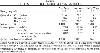
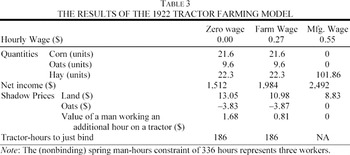
Once more, the marginal tractor hour generates more revenue than the marginal horse-team hour does, but now, the differences in the net income a farmer can generate by using tractors rather than horses becomes significant. In 1922 horse and tractor farming lead to approximately the same income, but by 1936 the farmer's net income is $263 greater if he utilizes tractors as opposed to horses. In 1922 the shadow value for horses and tractors drops so low with this high alternative wage that the optimum quantity of corn is zero. (The model implies that all the land should be put into hay if the alternative wage is above $0.42 or, alternatively, the farmer should leave farming and work in the industrial sector.) Even tractor farming in 1922 did not return as much as the average manufacturing wage of this time. In 1930 any wage over $0.49 would be better than growing corn or oats but by then tractor farming had become efficient enough so that at the $0.55 wage the optimum quantities again include corn and oats.

These results also indicate that, in the extreme case, a high manufacturing wage could encourage farmers to leave the farm, not buy a tractor! If the alternative wage is high enough, then the best solution for the farmer will be to exclusively work off the farm and sell or transfer the farm operation to someone whose comparative advantage in farming was greater.

The similarity of the horse and tractor revenue in 1922 and the widening gap between the two over time makes it easy to see that farmers were not slow to adopt tractors; they adopted them as the spread between the maximum revenue from tractor farming and horse farming grew larger and larger. This pattern is consistent with the pattern in the data: few farmers adopted tractors before 1930, but twice as many adopted them by 1940, and twice again as many adopted them by 1950. So the notion of farmers being slow to change is in reality not true. They only changed when the incentives were positive, not because markets did not function effectively, or because exogenous monetary shocks prevented them from doing so as previous authors have argued.

This last experiment using the manufacturing wage serves to illustrate the motivations for the huge structural changes that have rumbled through American agriculture to the present time: farm size grew, the number of livestock increased and the rural population dropped precipitously. This change was a combination of farmers taking jobs off the farms, or increasing their acreage, or spending more time with livestock. Although only 18.3 percent of farmers reported work off the farm for pay in 1930 (the first year of the record), by 1950, 30 percent did so. The number of farms began falling during the 1940s, and by 1960 there were only 174,707 farms on the same land area that had held 221,986 in 1935.

Hybrid Corn Experiment

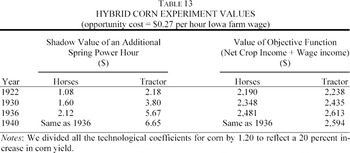
To further test the sensitivity of the model, we ran one last experiment using recalculated a_ijks to see how biotechnological change affected the shadow values of horses and tractors. Throughout this study we held constant all but the technical coefficients for land use. As previously discussed, the technical coefficients drop as yields rise.

Hybrid corn began to be planted in the late 1930s, principally in Iowa.³²

Macy, Arnold, and McKibben, “Changes,” p. 15.

Estimates at the time were a 20 percent increase in yield.³³

Ryan and Gross, “Acceptance,” p. 668.

Using this estimate, we recalculate the a_ijks as if the average corn yield had been 20 percent higher during the entire period (see Table 13). The maximum income rises $200 to $300 in each period. (We assume here that the price of corn remained constant; of course, as hybrid corn led to greater yields, the real price of corn would have dropped). The optimum quantity of corn rises 20 percent, as expected, but the optima for oats and hay are unchanged. There is a dramatic change in the shadow values. The increased yield on the land planted with hybrid corn has the effect of lowering input levels per unit of output. As long as the number of acres is constant, these lower a_ijks will not reduce the labor input. The larger yield raises the income possible per acre and so raises the shadow values of the nonpriced inputs. These rising shadow values mean that the alternative wage can rise much higher before it entices farmers completely from the farm. If higher yields lead to higher incomes, the price of the land will rise with them. Farmers who are less efficient may be enticed from their farms because manufacturing wages rise, or their land values rise.

CONCLUSIONS

The results from these linear programming models give a simpler and clearer understanding of the motivations for changing technologies. Previous applications of the threshold models, by focusing only on the cost of raising crops, failed to adequately quantify the opportunity cost of the farmer's time. In the 1920s and 1930s tractors did not produce more corn; they produced more time for the farmer. The cost of raising crops with tractors versus horses was not very different. The switch to tractors was a result of giving the farmer more time to engage in productive activities other than crops. With these results explanations such as market imperfections (which can be brought in to explain almost anything) and “lumpiness” of the inputs are not needed. The slow cumulative adoption can be explained by looking at the problem from the perspective of maximizing total net income, not just crop income. To maximize their income in a year, farmers look for the most efficient inputs to their field crop operation and use the saved time to earn greater income in some other activity or off-farm job.

In this article we have not touched on some interesting problems, for example, how the decision to invest in tractor technology might have been influenced by whether the farm was owner-operated or leased, or institutional constraints of that period.³⁴

See, for example, Whatley, “Southern Agrarian,” pp. 45–70.

In addition, family size might have mattered, in terms of affecting both the availability of perhaps low-wage labor, and also the alleviation of agency problems associated with proper care and maintenance of horses and tractors. We leave these issues to future research.

Appendix: The Technical Coefficients—An Overview³⁵
Details of these calculations are available from the authors. They are published in Dinah Duffy Martini's Ph.D. dissertation, “Technological Change in U.S. Agriculture: The Case of Substitution of Gasoline Tractor Power for Horse Power,” University of Washington, Seattle Washington, 2003.

Each a_ijk in the model is the amount of input i necessary to produce one unit of output j in a season k. However, there are several tasks in each season. Thus, the inputs must be calculated at the task level and then summed over all the tasks performed in each season to obtain each a_ijk. Each of these task level calculations requires several data points:

The tasks in the farming practice
The machine that was used for the task
The power source needed to pull that machine
The time it took that power source to pull the machine across one acre
The number of times the task was repeated
The number of acres needed to produce one unit of output

As an example, we calculate the a_ijk for the labor needed in corn in the Spring using horses. The Spring tasks were plowing, disking harrowing, and planting. In 1930 the most common horse implement for plowing was four horses pulling a two-bottom plow.³⁶

McKibben, Hopkins and Griffin, “Changes,” table 8, p. 22.

L. A. Reynoldson et al. report that this unit could plow one acre in 2.38 hours.³⁷

Reynoldson et al., “Utilization,” table 8.

Because plowing was usually only done once, the total man-hours needed for plowing was 2.38 hours. This process is repeated for disking (1 hour), harrowing (0.6 hours), and planting (0.7 hours). The sum of these man-hours per acre for these tasks is 4.6 hours. This number times the number of acres to produce one unit of corn, 2.62, is 12.07, (ignoring rounding error) which is a₂₁₂.

To find the horse-hours needed for corn in the spring, the man-hours per acre for each task are multiplied by the number of horses in the team pulling the implement for each task.

THE RESOURCE LIMITS

In general, these limits were the same for horse and tractor farming because at the time the farmer makes the decision to switch he has all the inputs available for horse farming. The literature reports over and over that farmers did not reduce the number of horses or labor until they had operated the tractor for a year or more. Most of the input limits in farming are time based: the number of man-hours, the number of horse-hours, the number of tractor-hours. Because the length of time available to complete a set of tasks is limited to certain periods in the year and days are limited to 24 hours, no matter the power source, the hourly input limits will be the same in all the models.

We derive the first three limits (man-hours, horse-hours, and tractor-hours) mainly from issues of the Iowa Year Book of Agriculture (IYBA) for 1920 through 1940 and the Agriculture Censuses for 1920–1940.³⁸

Iowa State Department of Agriculture. “Iowa Year Book of Agriculture,” vols. 20–41.

The last two (cropland and oat/hay acres) come directly from the IYBA for the applicable year. However, in the end, we reduced these amounts parametrically in order to make the constraints just bind, so that we could derive a positive shadow price of these resources.

MAN-HOURS AVAILABLE CALCULATION

As mentioned earlier, the farmer has a very definite period during which a group of tasks must be completed. Tasks left undone or performed too late cause yields to drop or, worst case, the loss of the crop. This means that when the farmer is planning what crops and how much of each to plant he knows that he must be able to complete, say, the plowing and planting between 15 April and 25 May. He must be able to do all the necessary work himself or he must be able to hire the help to do it. To capture this complex relationship in the model we derive the number of hours available per worker in each season and the number of available workers. The number of hours available depends on:

the length of the period in which the tasks must be done
the number of days in that period on which work in the fields can be done
the number of hours per day
the number of workers

The general calculation for the man-hours available in any period is: the number of work days in the season × the hours in a work day × the number of workers.

The number of workdays in a season is the total days in the performance period less the number of days it rains. If there are delays, weekend days could become workdays (for the farmer and his family). In the months of May in the years from 1890 to 1922 there were between five and 16 days with more than 0.01 inches of rain in the month.³⁹

Ibid., applicable years.

The average was 10.2 days, which means that if ten days of the 30 were lost, 20 or so would be left to do the Spring tasks.⁴⁰

Thomas and Hopkins, “Costs,” p. 17.

This accords well with the statements of Thomas and Hopkins: “Most of the work in preparing the seedbed and planting corn occurs during the first 2 weeks in May. These operations are most effective during a very short period. The timeliness of the operations becomes an important means of reducing production costs by increasing yields when operations are performed during the optimum time limit.” Planning to accomplish the spring work in early May left some flexibility if the weather was uncooperative.

Hopkins et al. reported that most farmers work 12 hours a day and their paid or unpaid helpers work 11. Because all the farmers also raised livestock for market, 3–4 hours per day of chores must be done.⁴¹

Hopkins, Goodsell, and Buck, “Economic Study,” p. 38.

“Chores” are those routine livestock tasks such as feeding, milking, etc. Generally the farmer did the livestock work and his helper did the plowing or planting because the livestock chores require more skill, better judgment, and high trustworthiness.⁴²

Holmes, “Wages,” p. 74.

This meant that after the livestock were cared for, there were approximately ten hours left of the day to do the crop work.

HORSE-HOURS AVAILABLE CALCULATION

Horses could work eight to ten hours a day. They usually worked for four hours in the morning had an hour or two midday rest and then worked another four. If the days were hot, the work time was reduced to avoid killing the horses with heat exhaustion.

In 1930, a heat wave in July during the grain harvest killed 10,000 horses in just a few days.⁴³

Iowa State Department of Agriculture, “Iowa Year Book,” vol. 30, p. 569.

The censuses report the number of horses in each county and the number of farms reporting horses, thus the average number of horses per farm is easily derived. Farmers could lengthen their work days by using different teams during the day for longer periods. The farmer might work for 12 hours, but each individual team might only work six or seven. The available horse-hours are calculated by multiplying the number of horses by ten hours per workday and then by the number of workdays.

TRACTOR-HOURS AVAILABLE

The tractor-hours are calculated by multiplying the workdays in the season times 10–12 hours in a day. Generally the tractor-hours are very close to the man-hours. The tractors could theoretically be worked 24 hours a day, but because they require a man to operate them, the available hours are constrained by the available labor hours. We assume one tractor on each tractor farm because very few farms had more than one as shown in Appendix Table 1.⁴⁴

U.S. Bureau of the Census, “Sixteenth Census,” Agriculture table 11, p. 119.

We are grateful to Doug Allen, Yoram Barzel, Levis Kochin, Jeremy Atack, and two anonymous referees for their insightful comments. Any remaining errors are of course the authors' responsibility.

References

Ankli Robert H. 1980 “Horses vs. Tractors in the Corn Belt,” Agricultural History 54, no. 1 134– 48.Google Scholar

Buck R. K., John A. Hopkins, and C. C. Malone. 1940 “Dairy and Hog Farming in Northeastern Iowa.” Agricultural Experiment Station Iowa State College of Agriculture and Mechanic Arts Research Bulletin: 275. Ames, Iowa:

Chen H. Y., and A. C. Arny. 1941 “Crop Rotation Studies.” University of Minnesota Agricultural Experiment Station, 149: 1– 6.Google Scholar

Clarke Sally. 1991 “New Deal Regulation and the Revolution in American Farm Productivity: A Case Study of the Diffusion of the Tractor in the Corn Belt, 1920–1940.” This Journal 51, no. 1 101– 23.Google Scholar

Cort M. J. 1919 “Creameries in Iowa.” Iowa Year Book of Agriculture, vol. 20. Des Moines, IA,

Davidson J. Brownlee, and William H. Carter. 1934 “Harvesting Alfalfa with a Windrow Pick-up Baler.” Iowa Agricultural Experiment Station Bulletin, 322. Ames, IA:

Goodsell Wylie D. 1939 “Cost and Utilization of Power and Labor on Iowa Farms.” Iowa State College, Agricultural Experiment Station Research Bulletin 258. Ames, Iowa:

Griliches Zvi. 1957 “Hybrid Corn: An Exploration in the Economics of Technological change.” Econometrica 25, no. 4 501– 22.Google Scholar

Griliches Zvi, 1960 “Demand for a Durable Input: Farm Tractors in the U.S., 1921–57.” In Demand for Durable Goods, edited by Arnold C. Harberger, 181– 207. Chicago: University of Chicago,

Holmes C. L. 1922 “Wages of Farm Labor.” The University of Minnesota Agricultural Experiment Station Technical Bulletin 4. St. Paul,

Hopkins John A. 1929 “The Crop System in Iowa County.” Iowa Agricultural Experiment Station Bulletin, 261. Ames, IA,

Hopkins John A. 1941 “Changes in Technology and Employment in Agriculture.” WPA National Research Project, Report No. A-9, Philadelphia,

Hopkins John A. Jr., Wylie D. Goodsell, and R. K. Buck. 1941 “An Economic Study of the Baby Beef Enterprise in Southern Iowa.” Agricultural Experiment Station Iowa State College of Agriculture and Mechanic Arts Research Bulletin, 272, Ames, IA,

Iowa State Department of Agriculture. 1919–1940. 1919 “Iowa Year Book of Agriculture” vols. 20 through 41: 677. Des Moines: Iowa State Department of Agriculture,

Lew Byron. 2000 “The Diffusion of Tractors on the Canadian Prairies: The Threshold Model and the Problem of Uncertainty.” Explorations in Economic History 37, no. 2 189– 216.Google Scholar

Macy Loring K., Lloyd E. Arnold, and Eugene G. McKibben. 1938 Changes in Technology and Labor Requirements in Crop Production: Corn. Works Progress Administration, National Research Project, Report No. A-5, Philadelphia,

Manuelli Rodolfo E., and Ananth Seshadri. 2003 “Frictionless Technology Diffusion: The case of Tractors.” NBER Working Paper Series, 9604

McKibben Eugene G., and R. Austin Griffin. 1938 “Changes in Farm Power and Equipment: Tractors Trucks and Automobiles.” Report A-9: 110. Philadelphia,

McKibben Eugene G., John A. Hopkins, and R. Austin Griffin. 1939 Changes in Farm Power and Equipment: Field Implements. Works Project Administration, National Research Project. Report A-11, Philadelphia,

Olmstead Alan L., and Paul W. Rhode. 2001 “Reshaping the Landscape: The Impact and Diffusion of the Tractor in American Agriculture, 1910–1960.” This Journal 61, no. 3 663– 98.Google Scholar

Pond George A. 1926 “A Study of Dairy Farm Organization in Southeastern Minnesota.” Minnesota Agriculture Experiment Station Technical Bulletin 44. St. Paul,

Reynoldson L. A., W. R. Humphries, S. R. Speelman, E. W. McComas, and W. H. Youngman. 1933 “Utilization and Cost of Power on Corn Belt Farms.” USDA Technical Bulletin 384. Washington, DC: GPO,

Richey Frederick. 1935 The What and How of Hybrid Corn, USDA Farmer's Bulletin: 1744

Ryan Bruce, and Neal Gross, January 1950 “Acceptance and Diffusion of Hybrid Seed Corn in Two Iowa Communities.” Agricultural Experiment Station Iowa State College of Agriculture and Mechanic Arts Research Bulletin, 372. Ames, IA:

Sallee George A., George A. Pond, and C. W. Crickman. 1939 “Farm Organization for Beef Cattle Production in Southwestern Minnesota.” University of Minnesota Agricultural Experiment Station:138. St Paul,

Shaw Eldon E., and John A. Hopkins. 1939 “Trends in Employment, 1909–1936.” Works Project Administration, National Research Project. Report A-8, Philadelphia,

Shedd C. K., December 1940 “Machinery for Growing Corn.” USDA Circular No. 592, Washington, DC,

Silberberg Eugene, and Wing Suen. 2000 The Structure of Economics, 3rd ed. McGraw-Hill,

Thomas H. L., and John A. Hopkins. 1932 “Costs and Utilization of Corn in Seven Iowa Counties.” Agricultural Experiment Station Iowa State College of Agriculture and Mechanic Arts Bulletin, 289

Tolley H. R. and L. A. Reynoldson. December 1921 “The Cost and Utilization of Power on Farms Where Tractors Are Owned.” USDA Farmer's Bulletin 997, Washington, DC: GPO,

United States Department of Agriculture (USDA). 1957 Major Statistical Series of the U.S. Dept of Agriculture: How they are Constructed. Washington, DC: GPO,

Whatley Warren C. 1987 “Southern Agrarian Labor Contracts as Impediments it Cotton Mechanization.” This Journal 47, no. 1 45– 70.Google Scholar

White William J. III. 2000 “An Unsung Hero: The Farm Tractor's Contribution to Twentieth Century United States Economic Growth.” Ph.D. dissertation, the Ohio State University,

Williams Michael. 1985 Ford and Fordson Tractors. Poole, Dorset, England: Blandford Press,

Williams Robert C. 1987 Fordson, Farmall and Poppin' Johnny: A History of the Farm Tractor and Its Impact on America. Urbana: University of Illinois Press,

U.S. Bureau of the Census. 1930 “Fifteenth Census of the United States, Agriculture.” Washington, DC: Department of Commerce,

U.S. Bureau of the Census. 1941 “Sixteenth Census of the United States: Agriculture.” Washington, DC: Department of Commerce,

U.S. Bureau of the Census. 1960 Historical Statistics of the United States, Colonial Times to the Present. Washington, DC: GPO,