1 Introduction
Lien et al. (Reference Lien, Henyey, Ma and Yang2014) reported on observations of large shoaling internal solitary waves (ISW) in the South China Sea with subsurfaces cores, but did not successfully model them nor did they explain their existence. Here we elucidate conditions under which such waves may exist, based on solutions of the Dubreil–Jacotin–Long (DJL) equation, using background conditions motivated by the field observations.
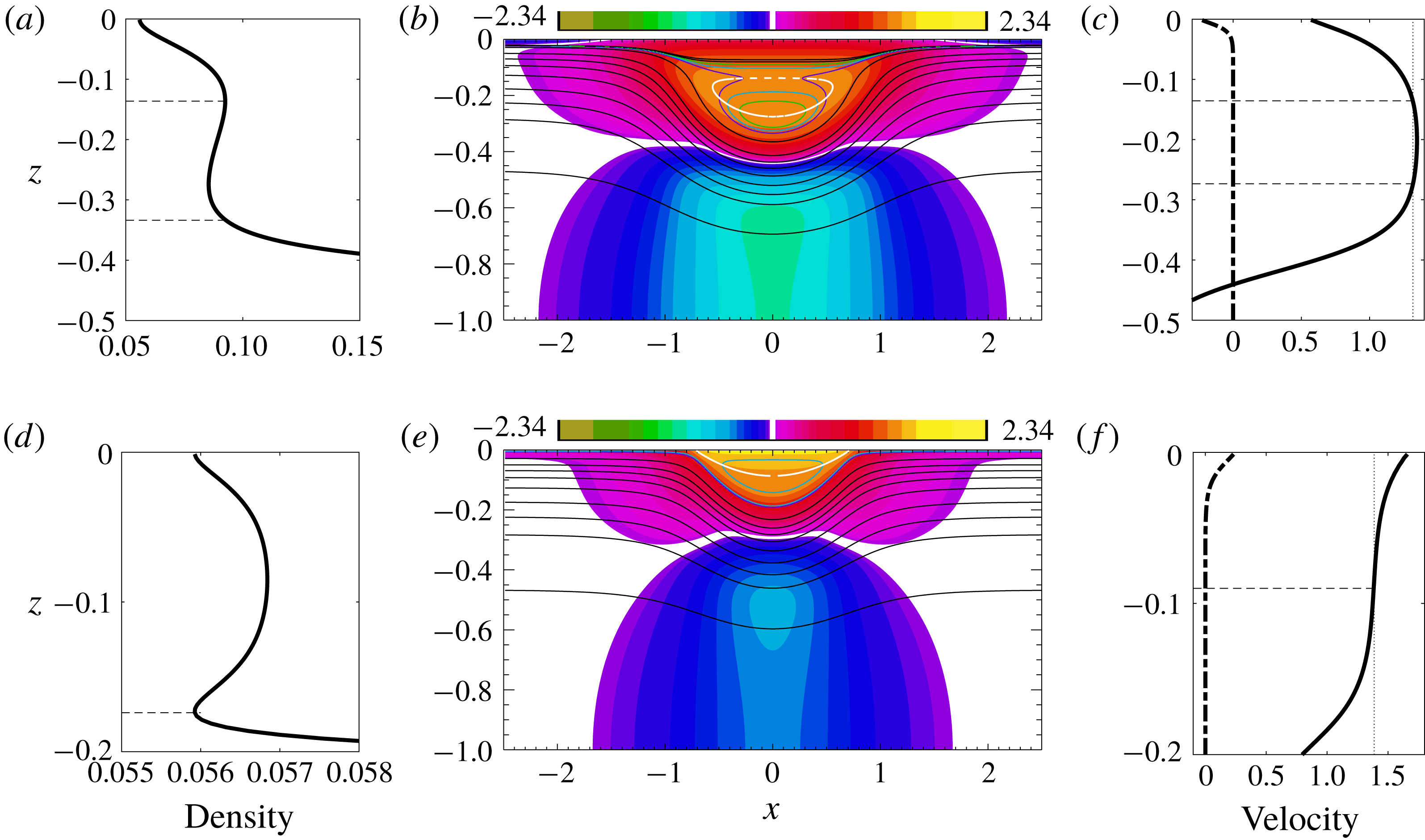
Figure 1(b,e) shows two mode-one ISW with cores computed by solving the DJL equation (Stastna & Lamb Reference Stastna and Lamb2002; Lamb Reference Lamb2003). The cores are the regions of closed density contours. The upper panel shows a wave whose core is below the surface, while the wave depicted in the lower panel has a core that is at the surface. These two waves were computed using the same background stratification but with different background currents (dash-dot curves in figure 1 c,f): the wave with a subsurface core (SSC) has near-surface vorticity of the opposite sign to the wave induced vorticity, while the wave with the surface core (SC) has background surface vorticity of the same sign. While the DJL equation is not strictly valid in the region of closed streamlines, these solutions are suggestive of the potential presence of core-like structures in ISW in the ocean, or in laboratory experiments, in which case these cores are dynamic, continually entraining and detraining fluid, and are expected to be highly turbulent particularly during the early stages of their life cycle. This dynamic nature is indicated by the presence of dense fluid overlying lighter fluid inside the DJL cores – such waves used as an initial condition in a time stepping model being convectively unstable. In this paper we use the occurrence of subsurface cores in DJL solutions to investigate conditions under which subsurface cores may exist in nature but we do not use them to make claims about the structure, stability or longevity of such cores. We confirm their existence in one example via a two-dimensional numerical simulation of a shoaling ISW.
Mode-one ISW are ubiquitous features in the world’s coastal oceans and large waves have occasionally been observed to have recirculating trapped cores (Lamb Reference Lamb2002, Reference Lamb2003; Klymak & Moum Reference Klymak and Moum2003; Scotti & Pineda Reference Scotti and Pineda2004; Lien et al. Reference Lien, Henyey, Ma and Yang2014). Together they provide an effective means of transporting fluid and particles, including plankton and suspended sediment. Previous numerical and theoretical work has considered waves with surface or bottom trapped cores in waves of depression and elevation, respectively. These cores are adjacent to the upper or lower boundaries. This paper reports on the conditions under which subsurface cores, lying well below the surface in internal solitary waves of depression, may exist.
Dimensionless mode-one internal solitary waves with cores (DJL solutions). Water depth is 1. (a–c) ISW with SSC. (d–f) ISW with SC. The base stratification shown in figure 2(a) was used. (b,e) Horizontal currents (colours) and evenly spaced density contours (black). The white contour lines are the
 $u=c$
contour. It passes through the centre of the core. The solid coloured contour lines are density contours chosen to indicate the core boundary, with closed contours being inside the core. (a,d) Density profiles down the centre of the wave. The horizontal dashed lines indicate the top and bottom of the core. In (d) the top boundary of the surface core is at the surface. (c,f) Horizontal current down the centre of the wave (solid) and the background current (dash-dot). The vertical dotted line indicates the wave propagation speed
 $c$
. Horizontal dashed lines indicated depths where
 $u=c$
.

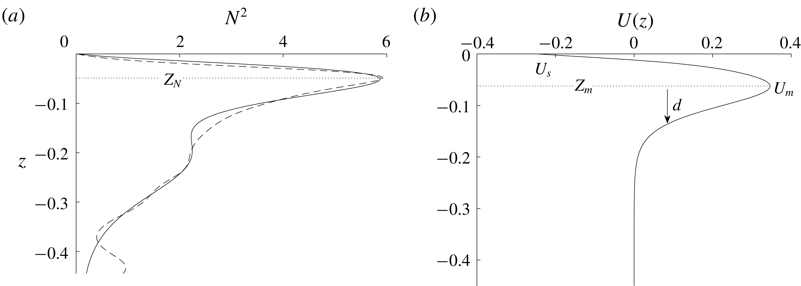
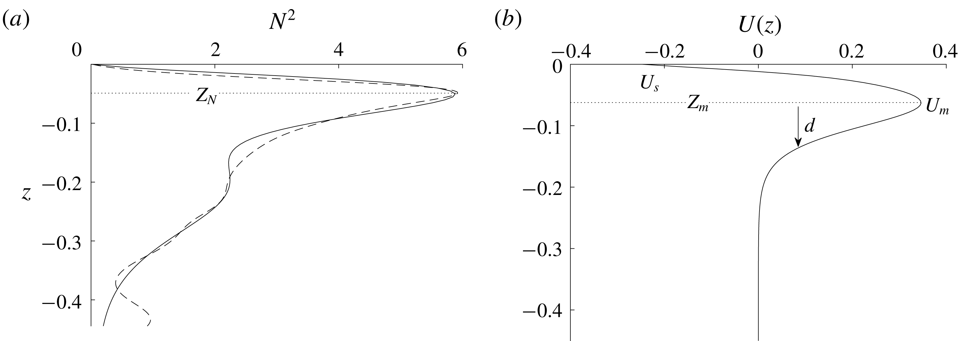
Background stratification and current profiles. (a) Stratification. The black dashed line is the observed stratification from 2 June and the black solid line is our base stratification. (b) Model current.
The first theoretical study of mode-one ISW with trapped cores dates back to the theoretical work by Derzho & Grimshaw (Reference Derzho and Grimshaw1997) who investigated the formation of cores in a nearly linear density (i.e., nearly constant buoyancy frequency) assuming a weakly nonlinear regime and a constant density, non-circulating core which is stagnant to leading order. In an investigation of shoaling waves of depression, Lamb (Reference Lamb2002) considered stratifications which increased monotonically towards the surface and found that waves with SCs always formed for large enough waves. This type of stratification profile is not common in the ocean and no background currents were included. Subsequently, Lamb (Reference Lamb2003) focused on a two-layer (hyperbolic-tangent) stratification and included a background current with shear confined to a surface layer. He only considered cases with waves of depression and background vorticity of the same sign as the wave induced vorticity and demonstrated the existence of waves with SCs if the background current shear at the surface was strong enough. Later Lamb & Wilkie (Reference Lamb and Wilkie2004) derived a theoretical model for conjugate flows (the horizontally homogeneous flow on the middle of long flat-crested solitary waves) with SCs. Choi (Reference Choi2006) was the first to study the existence of the stationary SSCs in ISW using a fully nonlinear model under the long wave approximation. He assumed a two-layer stratification with constant density and vorticity in each layer, and found that when the vorticity in the upper layer had the opposite sign to that of the wave-induced vorticity, a subsurface core could form. Work on ISW with cores was further extended by Helfrich & White (Reference Helfrich and White2010), where a theoretical model for large ISW with stagnant bottom cores, which included a density jump across the core boundary, was presented. Recently King, Carr & Dritschel (Reference King, Carr and Dritschel2011) presented a new numerical scheme for calculating the steady state form of ISW with cores in which the density is close to being constant inside the core. They did not include background currents.
Davis & Acrivos (Reference Davis and Acrivos1967) conducted the first experimental study of ISW with trapped cores. They considered mode-two solitary waves in a continuous two-layer stratification. It is fairly easy to generate cores in mode-two waves and most of the experimental work done since has focused on this situation (Kamachi & Honji Reference Kamachi and Honji1982; Stamp & Jacka Reference Stamp and Jacka1995; Sutherland & Nault Reference Sutherland and Nault2007). These waves have also been the subject of numerical investigations (Deepwell & Stastna Reference Deepwell and Stastna2016). Akylas & Grimshaw (Reference Akylas and Grimshaw1992) pointed out that stationary, theoretical mode-two ISW, regardless of the existence of cores, cannot generally be found due to resonance with short, trailing mode-one waves which drain energy from the leading wave. However, depending on the strength of the resonance, the model-two solitary-like waves can possibly be long-lived in a practical sense and have been observed in the ocean (Shroyer, Moum & Nash Reference Shroyer, Moum and Nash2010). Grue et al. (Reference Grue, Jensen, Rusas and Sveen2000) and Carr et al. (Reference Carr, Fructus, Grue, Jensen and Davies2008) experimentally generated mode-one ISW with trapped cores in a continuously stratified fluid. Recently Luzzatto-Fegiz & Helfrich (Reference Luzzatto-Fegiz and Helfrich2014) generated SCs with nearly uniform density and small circulation through dam break initial conditions. The experimental results are in good agreement with their viscous numerical simulations.
Observations of ISW with trapped cores are limited in the ocean, in part, because of difficulties in predicting their location and making measurements of sufficient accuracy to show that the maximum horizontal current exceeds the wave propagation speed (Lamb & Farmer Reference Lamb and Farmer2011; Lien et al. Reference Lien, Henyey, Ma and Yang2014; Zhang & Alford Reference Zhang and Alford2015). Klymak & Moum (Reference Klymak and Moum2003) and Scotti & Pineda (Reference Scotti and Pineda2004) made the first oceanic observation of trapped cores where large ISW of elevation with cores were found propagating along the ocean bottom. Recent observations of shoaling ISW of depression with a SSC were made in the South China Sea by Lien et al. (Reference Lien, D’Asaro, Henyey, Chang, Tang and Yang2012, Reference Lien, Henyey, Ma and Yang2014). These are the first detailed observations of oceanic waves of depression with trapped cores, where the wave properties, including amplitude, width and propagation speed were recorded. Waves of depression with cores have also been observed on the Washington continental shelf (Zhang & Alford Reference Zhang and Alford2015).
The presence of a background shear is well known to affect the generation and properties of ISW (Lamb Reference Lamb2010; Stastna & Walter Reference Stastna and Walter2014). Da Silva, New & Magalhaes (Reference Da Silva, New and Magalhaes2011) described the propagation characteristics of ISW with background shear by analysing a comprehensive set of SAR images in the western Indian Ocean. Bourgault, Galbraith & Chavanne (Reference Bourgault, Galbraith and Chavanne2016) reported an unexpected generation of ISW by frontally forced intrusions into a vertically sheared background environment and Walter et al. (Reference Walter, Stastna, Woodson and Monismith2016) reported on high-resolution observations of nonlinear internal waves at a coastal upwelling front. They found that theoretical solutions from the DJL equation did not accurately describe large ISW in strong shears possibly due to time varying background conditions. Hamann, Alford & Mickett (Reference Hamann, Alford and Mickett2018) examined the generation, propagation and dissipation of ISW in sheared currents over the Washington continental shelf. The three-dimensionality of the background current may have changed the propagation direction of the ISW inshore.
This paper is motivated by the observations made by Lien et al. (Reference Lien, Henyey, Ma and Yang2014). In their observations, large ISW with recirculating cores were found shoaling along the Dongsha slope, where the water depth was approximately 450 m. The amplitudes of the ISW were about 150 m and the heights of the cores, centred up to 100 m below the surface, occasionally exeeded 40 m. We will focus on the conditions under which SSCs can be formed in ISW of depression. Fully nonlinear ISW solutions of the DJL equation (Stastna & Lamb Reference Stastna and Lamb2002) are analysed, in which either SCs or SSCs can be formed depending on the background conditions. We find that the sign of the background current vorticity largely determines the location of the core, with near-surface vorticity of the same sign as the wave-induced vorticity leading to the formation of SCs while near-surface vorticity of the opposite sign is needed to form SSCs. Results from a two-dimensional numerical simulation of a shoaling ISW are also presented using background fields based on observations (Lien et al. Reference Lien, Henyey, Ma and Yang2014). The simulation results support the trapped core observation made by Lien et al. (Reference Lien, Henyey, Ma and Yang2014). Comparisons between these idealized numerical model results and the observations are made.
This paper is organized as follows. The equations of motion and numerical models are presented in § 2. The criteria for core formation in ISW calculated from the DJL solutions are described in § 3. Results of numerical simulations on shoaling waves are discussed in § 4. Our results are summarized and discussed in § 5.
2 Numerical models
We consider an incompressible, inviscid and non-rotating fluid under the Boussinesq approximation in two dimensions. The governing equations are
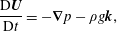 $$\begin{eqnarray}\displaystyle & \displaystyle \frac{\text{D}\boldsymbol{U}}{\text{D}t}=-\unicode[STIX]{x1D735}p-\unicode[STIX]{x1D70C}g\boldsymbol{k}, & \displaystyle\end{eqnarray}$$
 $$\begin{eqnarray}\displaystyle & \displaystyle \unicode[STIX]{x1D735}\boldsymbol{\cdot }\boldsymbol{U}=0, & \displaystyle\end{eqnarray}$$
 $$\begin{eqnarray}\displaystyle & \displaystyle \frac{\text{D}\unicode[STIX]{x1D70C}}{\text{D}t}=0, & \displaystyle\end{eqnarray}$$
where
 $\boldsymbol{U}(x,z,t)=(u,w)$
is the velocity vector with
 $u$
the horizontal velocity and
 $w$
the vertical velocity positive upwards,
 $(x,z)$
are the corresponding spatial coordinates,
 $t$
is time,
 $\text{D}/\text{D}t$
is the material derivative, and
 $\unicode[STIX]{x1D70C}$
and
 $p$
are the density and pressure perturbations which have been scaled by the constant reference density
 $\unicode[STIX]{x1D70C}_{0}$
making
 $\unicode[STIX]{x1D70C}$
dimensionless. For the numerical simulations considered in § 4 we solve the governing equations (2.1)–(2.3) using a second-order projection method (Lamb Reference Lamb2007). The model adopts terrain-following coordinates. A vertically varying resolution is used with higher vertical resolution near the surface where large density and current gradients are located. The rigid lid approximation is imposed on the water surface at
 $z=0$
.
We explore the conditions under which ISW with a SSC may exist through solutions of the DJL equation extended to include background currents (Stastna & Lamb Reference Stastna and Lamb2002; Lamb Reference Lamb2003) with a flat bottom at
 $z=-H$
. Let
 $\unicode[STIX]{x1D702}(x,z)$
denote the vertical displacement of the isopycnal (or streamline) passing through
 $(x,z)$
from its upstream position in a reference frame moving with the wave in which the flow is steady. Under the Boussinesq approximation the DJL equation is
 $$\begin{eqnarray}\displaystyle & \displaystyle \unicode[STIX]{x1D6FB}^{2}\unicode[STIX]{x1D702}-\frac{\bar{U}^{\prime }(z-\unicode[STIX]{x1D702})}{\bar{U}(z-\unicode[STIX]{x1D702})-c}[\unicode[STIX]{x1D702}_{x}^{2}+(\unicode[STIX]{x1D702}_{z}-2)\unicode[STIX]{x1D702}_{z}]+\frac{N^{2}(z-\unicode[STIX]{x1D702})}{(\bar{U}(z-\unicode[STIX]{x1D702})-c)^{2}}\unicode[STIX]{x1D702}=0, & \displaystyle\end{eqnarray}$$
 $$\begin{eqnarray}\displaystyle & \displaystyle \unicode[STIX]{x1D702}=0\quad \text{at }z=0,-H, & \displaystyle\end{eqnarray}$$
 $$\begin{eqnarray}\displaystyle & \displaystyle \unicode[STIX]{x1D702}\rightarrow 0\quad \text{as }|x|\rightarrow \infty . & \displaystyle\end{eqnarray}$$
Here
 $c$
is the unknown wave propagation speed,
 $N^{2}$
is the square of the Brunt–Väisälä frequency of the background state, and
 $\bar{U}$
is the background current with a prime denoting its derivative. The DJL equation is derived by following streamlines to the far-field flow and hence is uniquely determined only along open streamlines. Wave solutions with closed streamlines, or recirculating cores, can also be computed from the DJL equation, however the structure inside the cores are indeterminate (Tung, Chan & Kubota Reference Tung, Chan and Kubota1982; Brown & Christie Reference Brown and Christie1998). As a result, the DJL equation can predict the existence of a core, the presence of which is indicated by
 $U_{max}\geqslant c$
where
 $U_{max}$
is the maximum current in the wave, but the flow inside the core, and hence the detailed structure of the solitary waves with a core, are not physically correct. We solve the DJL equations (2.4)–(2.6) following the approach of Stastna & Lamb (Reference Stastna and Lamb2002), which is based on the method of Turkington, Eydeland & Wang (Reference Turkington, Eydeland and Wang1991).
3 DJL solutions
We investigate what background conditions allow for the formation of SSCs in DJL solutions, using this as a proxy for conditions under which unsteady SSCs may exist in nature. In particular, we focus on waves of depression with trapped cores using a
 $\text{sech}^{2}$
shaped background current profile and a simple stratification fitted to the observations made by Lien et al. (Reference Lien, Henyey, Ma and Yang2014) on the 2 June (note Lien et al. (Reference Lien, Henyey, Ma and Yang2014) based their DJL solution from their 3 June observations which had a slightly lower pycnocline). The observed stratification and currents are characterized by a thin pycnocline close to the surface and a subsurface current, or jet, in the direction of wave propagation. The primary significance of the latter feature is that the near-surface vorticity has the opposite sign to that induced by the ISW, although current observations did not go all the way to the surface. Our background fields are based on these characterizations of the observations.
We consider five parameters which are indicated in figure 2:
 $Z_{N}$
, the vertical location of the maximum buoyancy frequency;
 $d$
, the width of the background current;
 $U_{s}$
, the current at the surface;
 $U_{m}\geqslant 0$
, the maximum velocity of the subsurface jet; and
 $Z_{m}$
, the location of
 $U_{m}$
. Our model current goes to zero well above the bottom.
The problem is non-dimensionalized using the water depth
 $H$
as the length scale,
 $\bar{c}=\bar{N}H/\unicode[STIX]{x03C0}=\sqrt{g\unicode[STIX]{x1D6FF}\unicode[STIX]{x1D70C}H}/\unicode[STIX]{x03C0}$
, where
 $\bar{N}$
is the square root of the average of
 $N^{2}$
, as the velocity scale (
 $\bar{c}$
would be the linear long wave propagation speed for a uniform stratification) and
 $H/\bar{c}$
as the time scale. Here,
 $\unicode[STIX]{x1D6FF}\unicode[STIX]{x1D70C}$
is the dimensionless density change over the water column and
 $g$
is the gravitational acceleration. The stratification and the background current profiles are given by
 $$\begin{eqnarray}\displaystyle \bar{\unicode[STIX]{x1D70C}}(z) & = & \displaystyle 0.37\left(1.0-\tanh \left(\frac{z-Z_{N}+0.01}{0.06}\right)\right)-0.11\left(1.0-\tanh \left(\frac{z}{-0.022-Z_{N}}\right)\right)\nonumber\\ \displaystyle & & \displaystyle +\,0.23\left(1.0-\tanh \left(\frac{z+0.16-Z_{N}}{0.11}\right)\right)-0.0002(z-Z_{N}-0.05),\end{eqnarray}$$
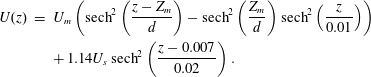 $$\begin{eqnarray}\displaystyle U(z) & = & \displaystyle U_{m}\left(\text{sech}^{2}\left(\frac{z-Z_{m}}{d}\right)-\text{sech}^{2}\left(\frac{Z_{m}}{d}\right)\text{sech}^{2}\left(\frac{z}{0.01}\right)\right)\nonumber\\ \displaystyle & & \displaystyle +\,1.14U_{s}\,\text{sech}^{2}\left(\frac{z-0.007}{0.02}\right).\end{eqnarray}$$
To investigate the influence of these five parameters, a base case is set up using
 $(Z_{N},d,U_{s},U_{m},Z_{m})=(-0.05,0.055,-0.24,0.35,-0.06)$
(see figure 2). We computed DJL solutions for 10 sets of waves to examine how the five parameters affect the existence of a core. In each of the 10 sets, two parameters are varied. Two values of
 $Z_{N}$
are used,
 $-0.05$
and
 $-0.067$
. Ranges for the other four parameters are:
 $U_{m}\in [0.0,0.35]$
,
 $Z_{m}\in [-0.2,-0.038]$
,
 $U_{s}\in [-1.5,0.18]$
and
 $d\in [0.024,0.18]$
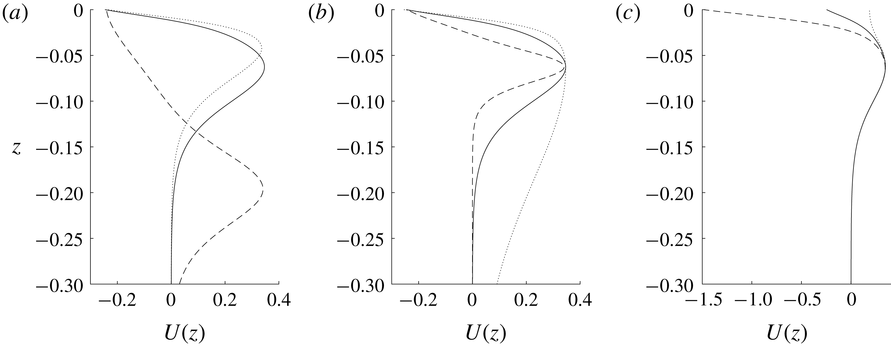
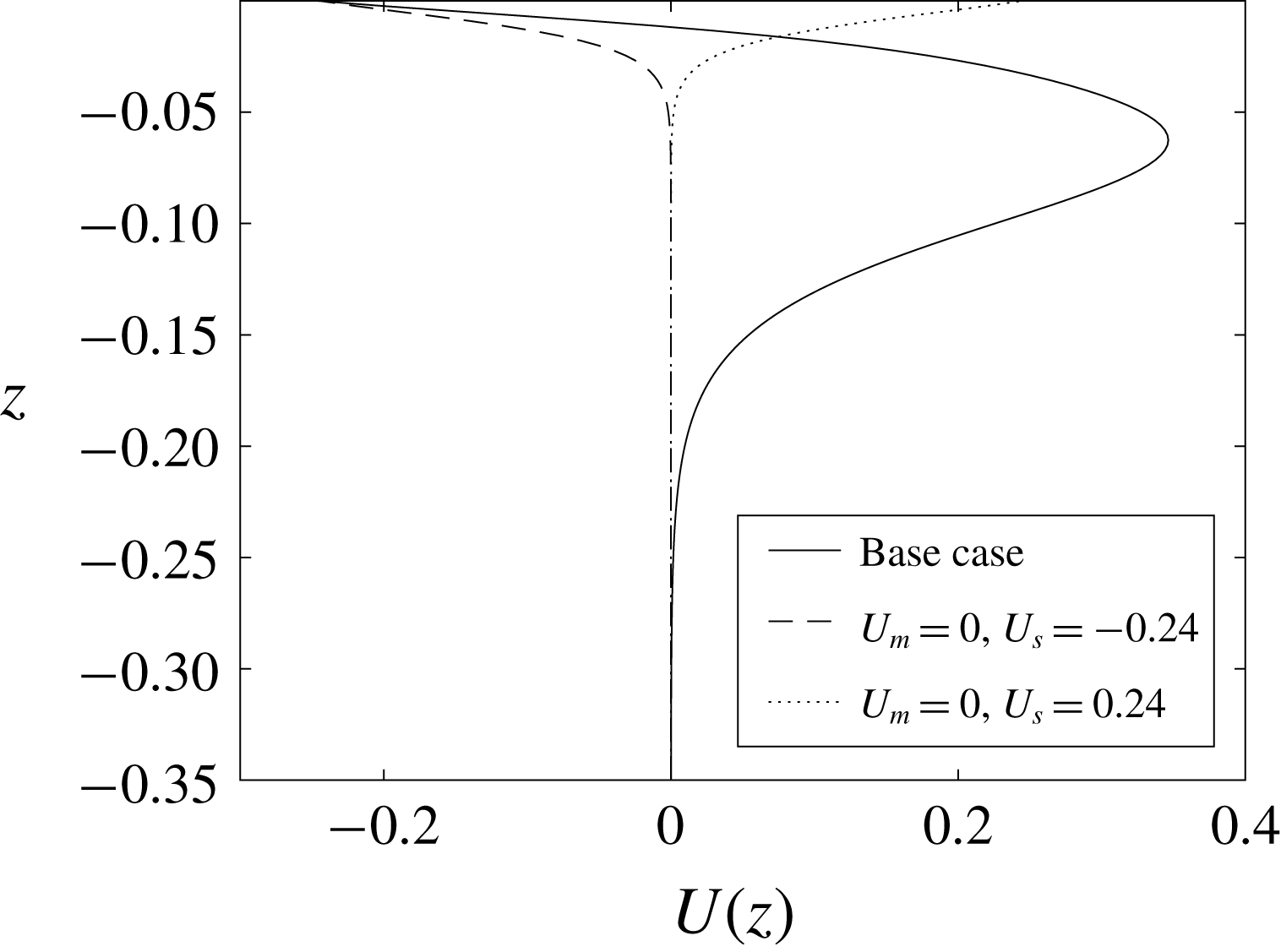
. Figure 3 gives examples of different background currents.
Example background current profiles. The black solid line is the base case. The dashed and dotted lines are for (a)
 $Z_{m}=-0.2$
and
 $-0.038$
, (b)
 $d=0.024$
and 0.18, (c)
 $U_{s}=-1.5$
and 0.18.
3.1 Criteria for core formation
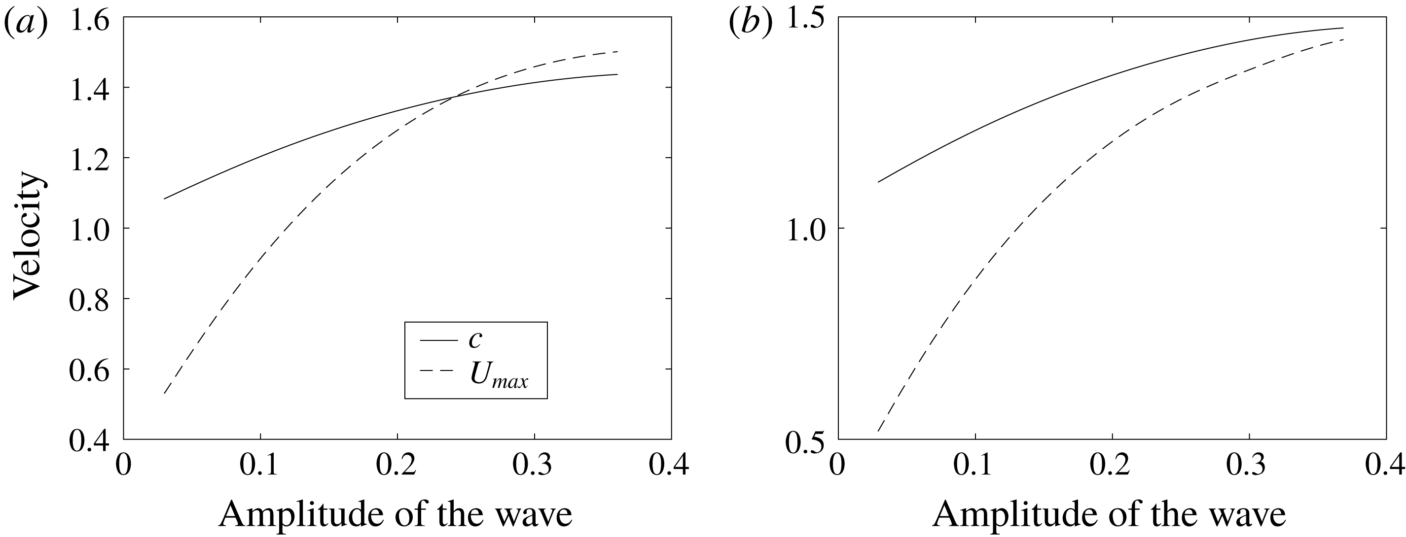
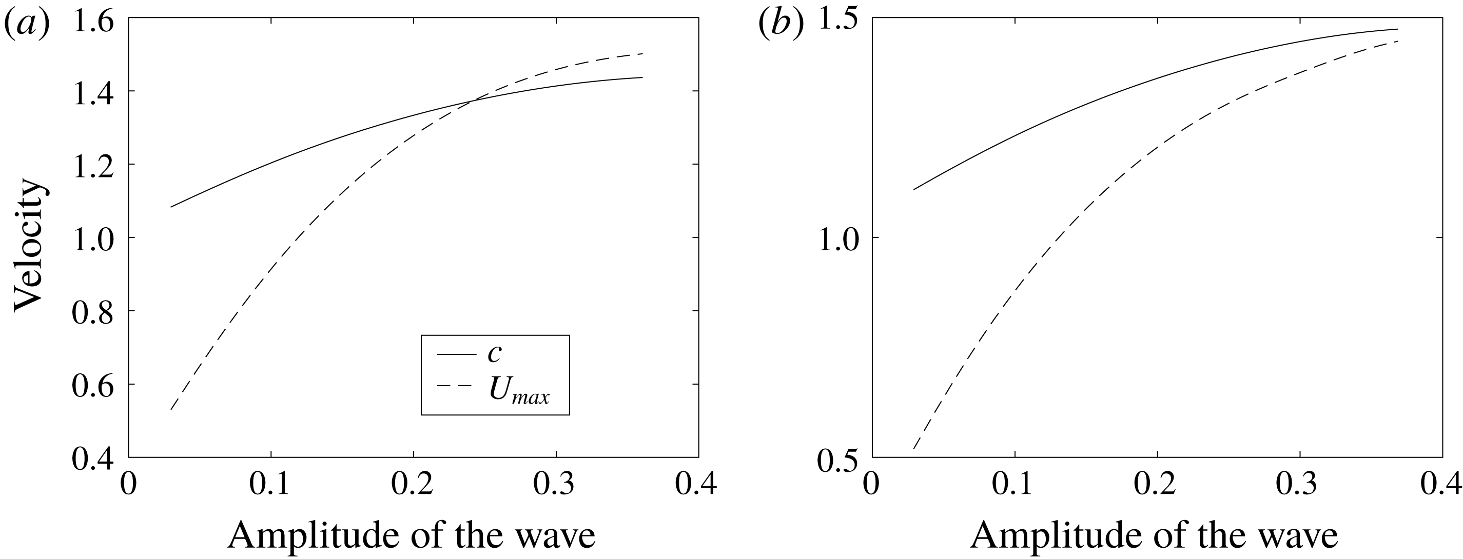
All DJL solutions have similar features regarding the presence of cores. For sufficiently small amplitude/energy waves, the maximum horizontal fluid velocity
 $U_{max}$
is smaller than the propagation speed
 $c$
. As the wave amplitude/energy increases, both
 $c$
and
 $U_{max}$
increase. If the fluid velocity surpasses the wave propagation speed, i.e., the curves of
 $c$
and
 $U_{max}$
intersect (figure 4
a), a core is present. The size of the core and the difference between
 $U_{max}$
and
 $c$
increase as the wave amplitude continues to increase. The ISW generally have a limiting amplitude. For example, for a two-layer stratification with an interface, in the absence of a background current the amplitude is limited by the distance of the interface from the mid-depth. If the limiting amplitude is reached with
 $U_{max}<c$
(figure 4
b) a core is not formed. It is important to note that while the structure of the flow inside the core is not accurately modelled by the DJL equation (in particular the flow inside an ISW core is not steady), ISW with open streamlines cannot exist with amplitudes exceeding that at which
 $U_{max}=c$
.
Maximum horizontal current
 $U_{max}$
and wave propagation speed
 $c$
. (a) The base case. (b) Case with
 $U_{s}=0.18$
and all other parameters as for the base case (see figure 3
c). For this case the maximum wave amplitude of about 0.37 is reached without the formation of a core.
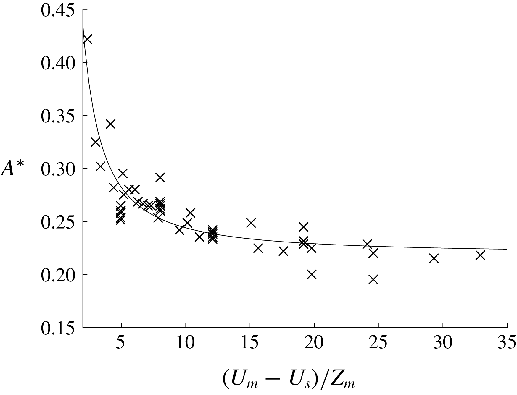
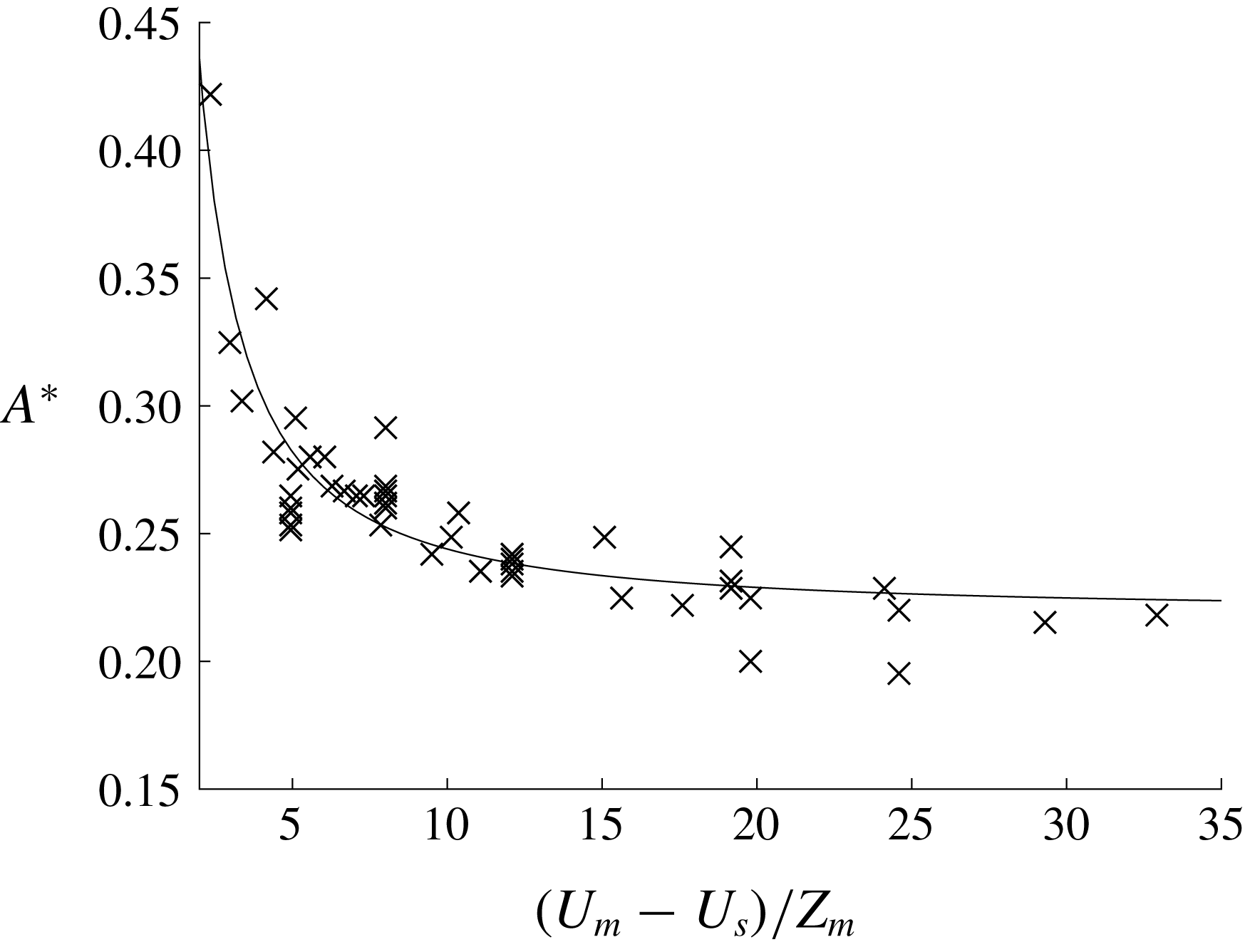
In addition to the aforementioned general features, we find that cores are easier to form if the magnitude of the background near-surface vorticity is increased. We denote the minimum wave amplitude necessary for core formation as
 $A^{\ast }$
(i.e., the wave amplitude at which
 $U_{max}=c$
). The surface vorticity can be approximated by
 $\unicode[STIX]{x1D701}_{a}=(U_{m}-U_{s})/Z_{m}$
. As
 $\unicode[STIX]{x1D701}_{a}$
increases,
 $A^{\ast }$
decreases and it is easier to form a core. In figure 5, we plot the data from all cases using the base stratification, where
 $A^{\ast }$
is plotted as a function of
 $\unicode[STIX]{x1D701}_{a}$
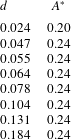
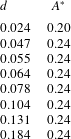
. The formation of a core is not very sensitive to the thickness
 $d$
of the subsurface jet (see table 1).
Plot of
 $(U_{m}-U_{s})/Z_{m}$
versus
 $A^{\ast }$
using the base stratification. The black solid line is a fitted curve.
Base stratification is used and
 $U_{m}-U_{s}$
is fixed at 0.6.
 $d$
is varied and
 $A^{\ast }$
is the corresponding minimum wave amplitude required to generate a core.
3.2
 $U_{m}=0$

We now consider the simpler case where
 $U_{m}=0$
in (3.2). In these cases the background shear is single-signed and non-zero only in a surface layer (figure 6). This current is of a similar structure to that in Lamb (Reference Lamb2003) however both negative and positive near-surface vorticity are now considered. The other difference is that Lamb used a much lower pycnocline centred at about
 $z=-0.32$
with a buoyancy frequency near the surface close to zero. As a result, all the cores generated in Lamb (Reference Lamb2003) were SCs. The DJL solutions with a SC and a SSC shown in figure 1 used
 $U_{m}=0$
and positive and negative values of
 $U_{s}$
, respectively.
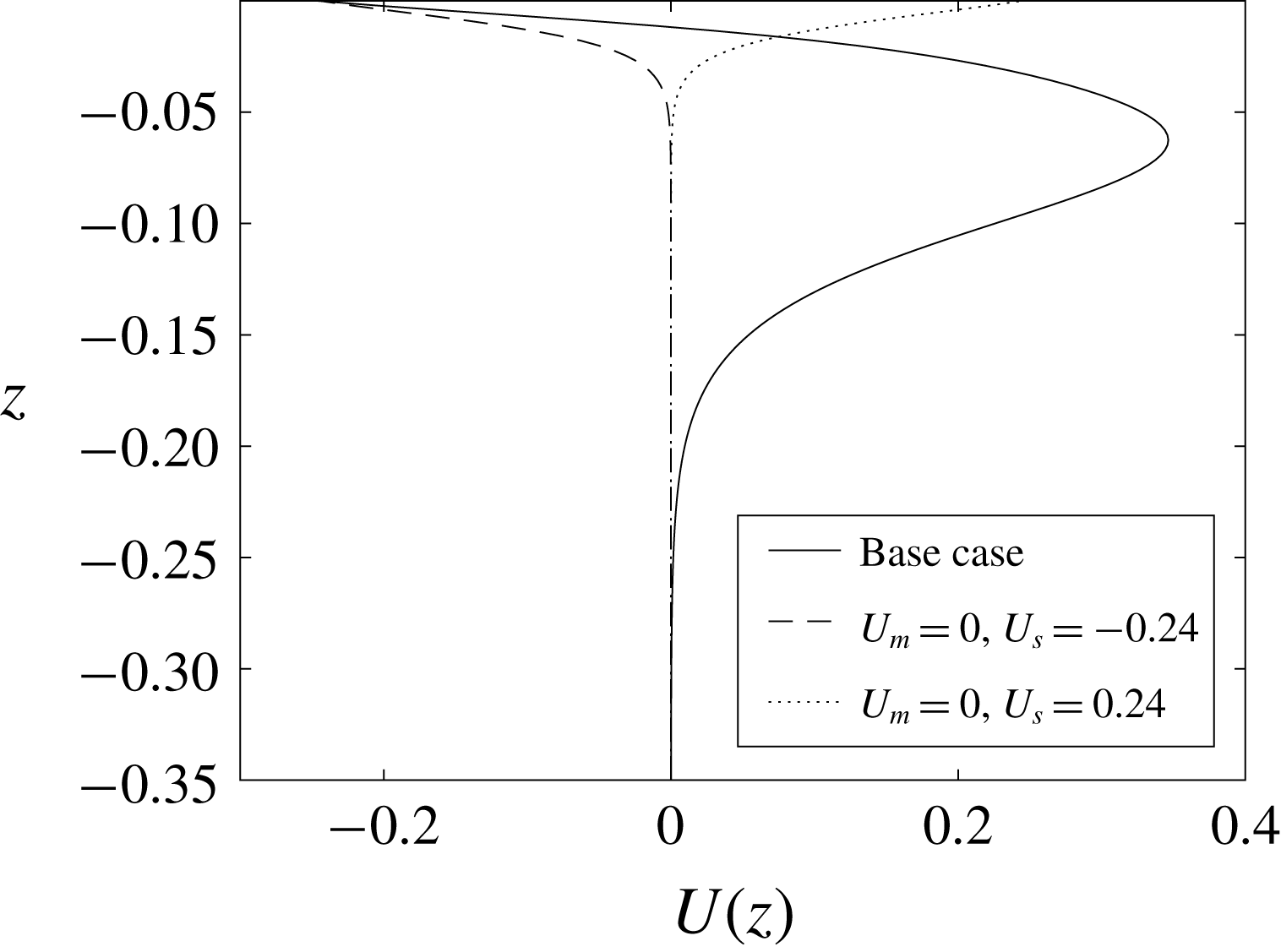
Background current profiles with
 $U_{m}=0$
:
 $U_{s}=-0.24$
(dashed) and
 $U_{s}=0.24$
(dotted)). Also shown is the base current profile (solid).
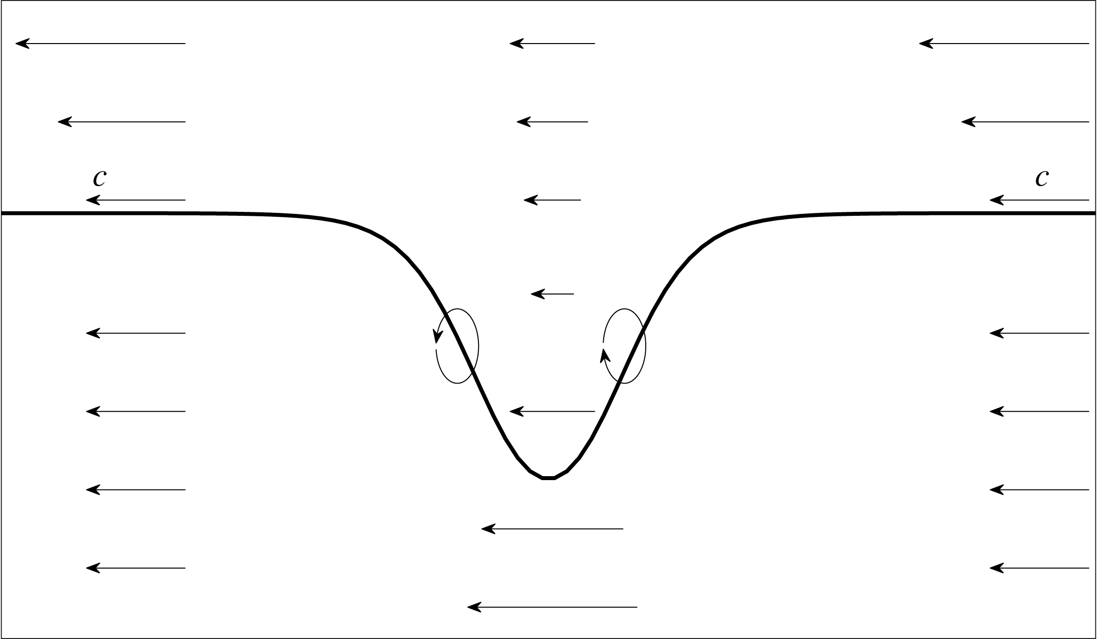
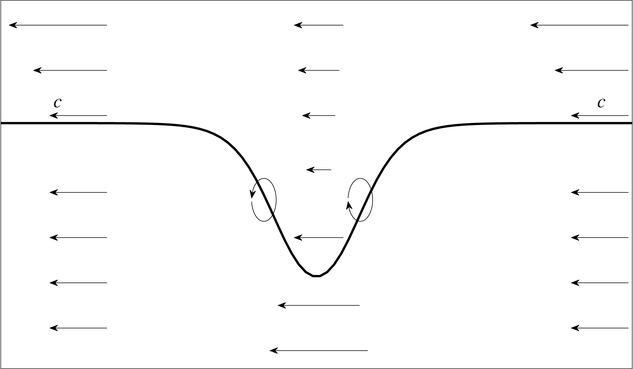
A schematic plot of a wave of depression propagating to the right. The reference frame is moving with the wave with its phase speed
 $c$
. The background current here has a negative near-surface vorticity. The ellipses indicate how the vorticity is changing in the front and back halves of the wave.
We find that the sign of the near-surface vorticity of the current determines the core location. SCs are formed when the vorticity of the background current and that generated by the ISW are of the same sign. SSCs are formed when the signs differ. Two sets of simulations were conducted which confirmed this hypothesis. The first set used the base stratification and the second used a stratification with a much lower pycnocline (at
 $z=-0.17$
). Currents with positive or negative vorticity were used for both sets. We also found that generally the generation of the SSC is more sensitive to the magnitude of the vorticity of the current and the location of the pycnocline than the generation of the SC. As the pycnocline is lowered, for waves of fixed amplitudes, the near-surface isopycnals have smaller displacements and a thin near-surface layer of vorticity has less influence on the wave. Since SSCs are lower in the water column than SCs, lowering the pycnocline affects the SSCs more.
3.3 Vorticity generation mechanism
Here we provide a simple explanation of how the background current profile determines the location of the core. We consider a wave of depression propagating to the right using a reference frame moving with the wave (figure 7). The vorticity equation for our two-dimensional inviscid flow is
 $$\begin{eqnarray}\displaystyle \frac{\text{D}\unicode[STIX]{x1D714}}{\text{D}t}=\unicode[STIX]{x1D70C}_{x}g. & & \displaystyle\end{eqnarray}$$
In the front half of a wave of depression, the sloping isopycnals have positive
 $\unicode[STIX]{x1D70C}_{x}$
hence the vorticity
 $\unicode[STIX]{x1D714}=u_{z}-w_{x}$
of a fluid particle increases as it enters the wave, reaching a maximum at the wave centre, thereafter decreasing to its original value as it passes through the rear half of the wave where
 $\unicode[STIX]{x1D70C}_{x}$
is negative.
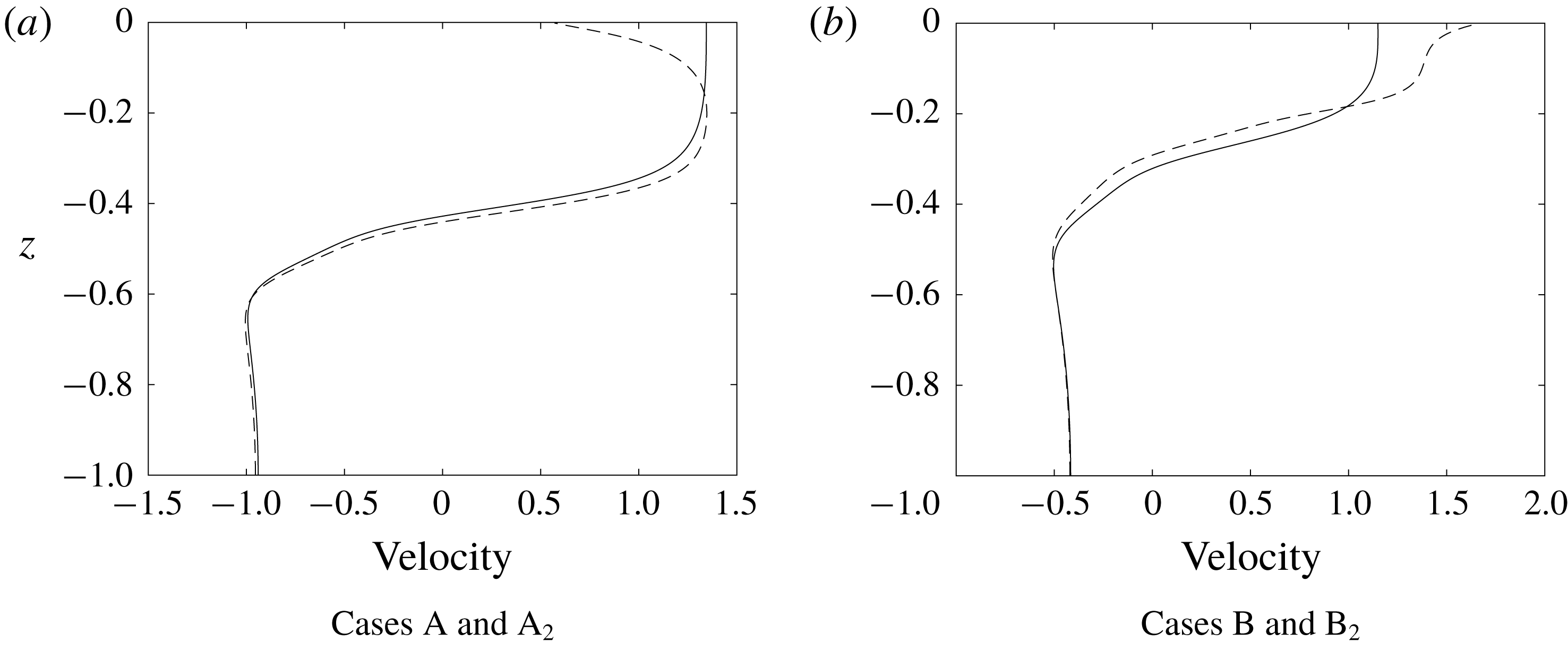
In figure 8, we compare the horizontal velocity profiles down the centre of the wave for four waves using the base stratification. Waves A and B are the waves shown in figure 1(b,e) which use background currents with negative and positive near-surface vorticity, respectively. There is no background current in cases A
 $_{2}$
and B
 $_{2}$
and, as a result, no cores are generated. The four waves have similar but not identical amplitudes.
Horizontal velocity profiles down wave centres. (a) Case A with negative near-surface background vorticity (dashed), and case A
 $_{2}$
with no background current (solid). (b) Case B with positive near-surface background vorticity (dashed), and case B
 $_{2}$
with no background current (solid).
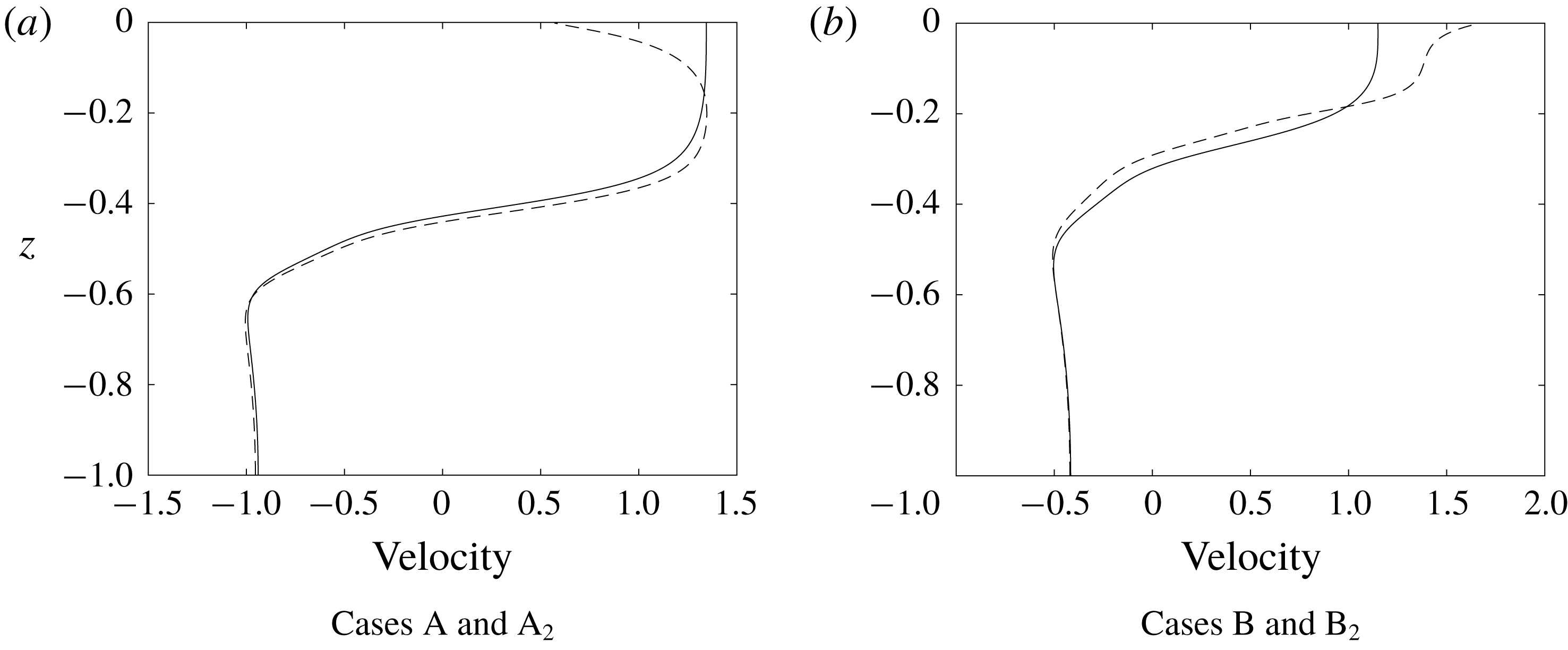
The waves in cases A and B have negative and positive near-surface vorticity in their centres while waves A
 $_{2}$
and B
 $_{2}$
have little near-surface shear. This difference in near-surface vorticity is a result of the differences in the vorticity of the background current and the weak near-surface baroclinic generation of vorticity: if the baroclinic generation is weak in the near-surface layer then the vorticity in this layer in the wave will be similar to that of the background current outside of the wave.
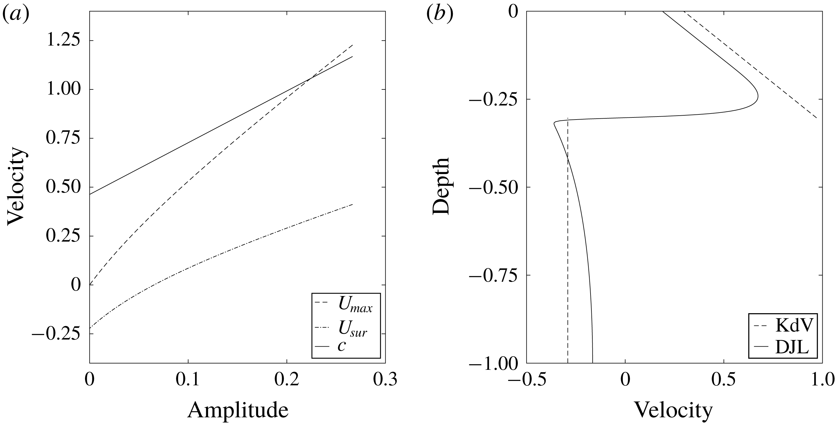
While this explains the subsurface current maximum when the background current has negative near-surface vorticity, it does not on its own predict that the subsurface maximum current can exceed the propagation speed of the wave, a necessary condition for the formation of a SSC. This occurs because the forward volume flux in the upper part of the wave (e.g., above the main pycnocline) must be equal and opposite to that below. As the wave amplitude increases this mean value increases and the subsurface current maximum increases as well. A simple idealized two-layer model combined with the Korteweg–de Vries (KdV) equation predicts just this.
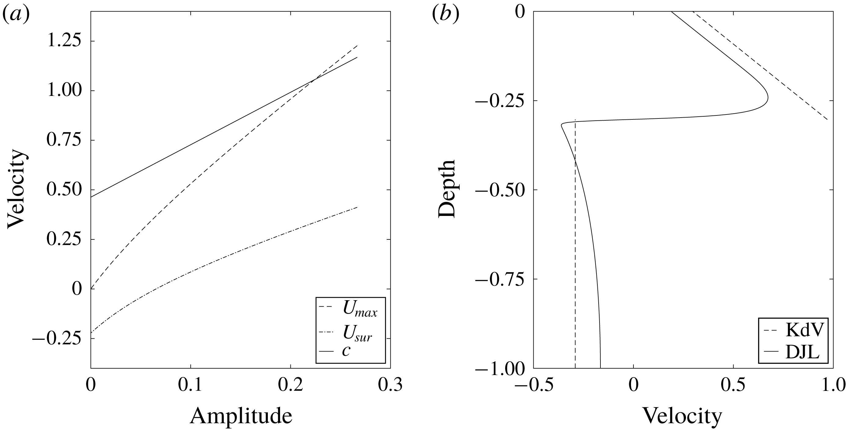
KdV solutions. (a)
 $U_{max}$
(dashed),
 $U_{sur}$
(dash-dotted) and
 $c$
(solid) predicted by KdV theory. (b) Velocity down the centre of the wave obtained from the DJL solution (solid) and the KdV equation (dashed). The wave amplitude is 0.2.
Consider two layers of constant density and a continuous background current which is zero in the lower layer and has constant vorticity in the upper layer. That is,
 $$\begin{eqnarray}\displaystyle & \displaystyle \unicode[STIX]{x1D70C}(z)=1-H(z+h_{1}), & \displaystyle\end{eqnarray}$$
 $$\begin{eqnarray}\displaystyle & \displaystyle \bar{U}(z)=U_{s}\left(1+\frac{z}{h_{1}}\right)H(z+h_{1}), & \displaystyle\end{eqnarray}$$
where
 $H(z)$
is the Heaviside function,
 $h_{1}$
is the depth of the upper layer and
 $U_{s}$
is the background current at the surface. KdV theory gives the wave propagation speed
 $c=c_{0}+(a\unicode[STIX]{x1D6FC}/3)$
(Ostrovsky & Stepanyants Reference Ostrovsky and Stepanyants1989), where
 $a$
is the interface displacement and
 $c_{0}$
is the linear long wave phase speed given by
 $$\begin{eqnarray}\displaystyle c_{0}=\frac{h_{2}U_{s}\pm \sqrt{h_{2}^{2}U_{s}^{2}+4h_{1}h_{2}g^{\prime }}}{2}, & & \displaystyle\end{eqnarray}$$
where
 $h_{2}=1-h_{1}$
is the depth of the lower layer and
 $g^{\prime }$
, the reduced gravity, is equal to one with our non-dimensionalization. The nonlinear coefficient
 $\unicode[STIX]{x1D6FC}$
is
 $$\begin{eqnarray}\displaystyle \unicode[STIX]{x1D6FC}=\frac{-3h_{2}^{2}c_{0}^{2}+3h_{2}^{2}U_{s}c_{0}-h_{2}^{2}U_{s}^{2}+3h_{1}^{2}c_{0}^{2}}{(2h_{2}c_{0}-h_{2}U_{s}+2h_{1}c_{0})h_{1}h_{2}}. & & \displaystyle\end{eqnarray}$$
If we assume the solitary waves are very broad so that the vorticity in the centre of the wave is well approximated by
 $u_{z}$
and apply conservation of volume flux, we obtain the following horizontal velocity profile down the centre of the wave
 $$\begin{eqnarray}u_{c}(z)=u_{2}+\left[u_{1}-u_{2}+\frac{U_{s}h_{1}}{2(h_{1}-a)}+\frac{U_{s}}{h_{1}}\left(z+\frac{h_{1}-a}{2}\right)\right]H(z+h_{1}-a),\end{eqnarray}$$
where
 $u_{1}=-ac/h_{1}-a$
and
 $u_{2}=ac/h_{2}+a$
are the velocities in the centre of the wave above and below the pycnocline, respectively, when there is no background current. Here the vorticity in the wave is equal to that of the background current, a result of each layer having constant density.
We use the KdV solution to illustrate some interesting patterns of the velocity profile down the centre of the wave. In our simple two-layer system,
 $U_{max}=u_{c}(-h_{1}^{+}+a)$
, where the
 $h_{1}^{+}$
indicates that it is evaluated above the interface, and
 $U_{sur}=u_{c}(0)$
. Figure 9(a) plots
 $U_{max}$
,
 $U_{sur}$
and
 $c$
. As the wave amplitude gets larger,
 $U_{max}$
increases more quickly than
 $U_{sur}$
, predicting the formation of a core when they cross. Note, however, that KdV theory is weakly nonlinear and becomes inaccurate when the wave gets too large. Figure 9(b) plots the horizontal velocity down the centre of the wave. The KdV solution manages to capture the behaviour of the near-surface vorticity, though it over-predicts the magnitude of the velocity.
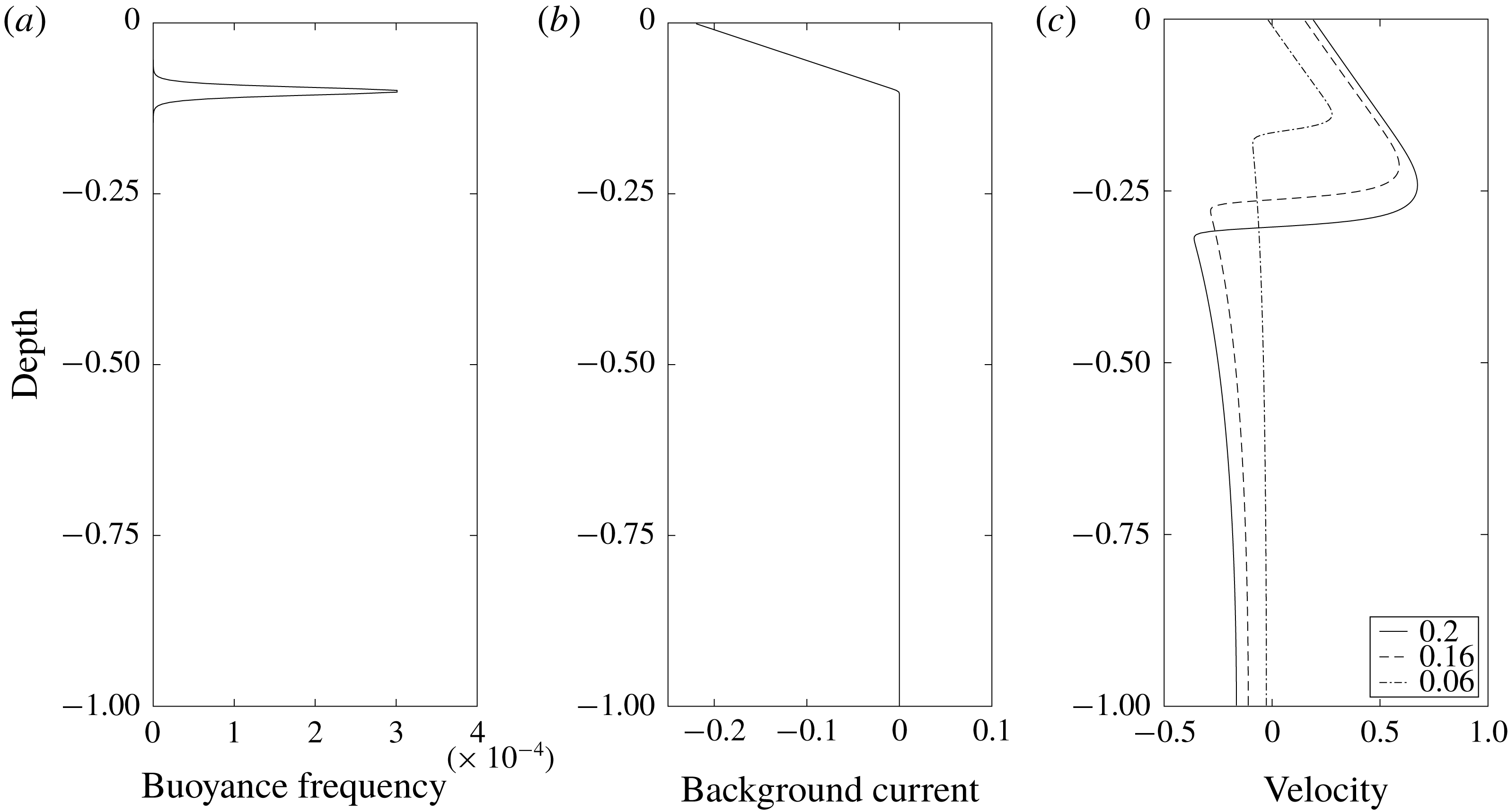
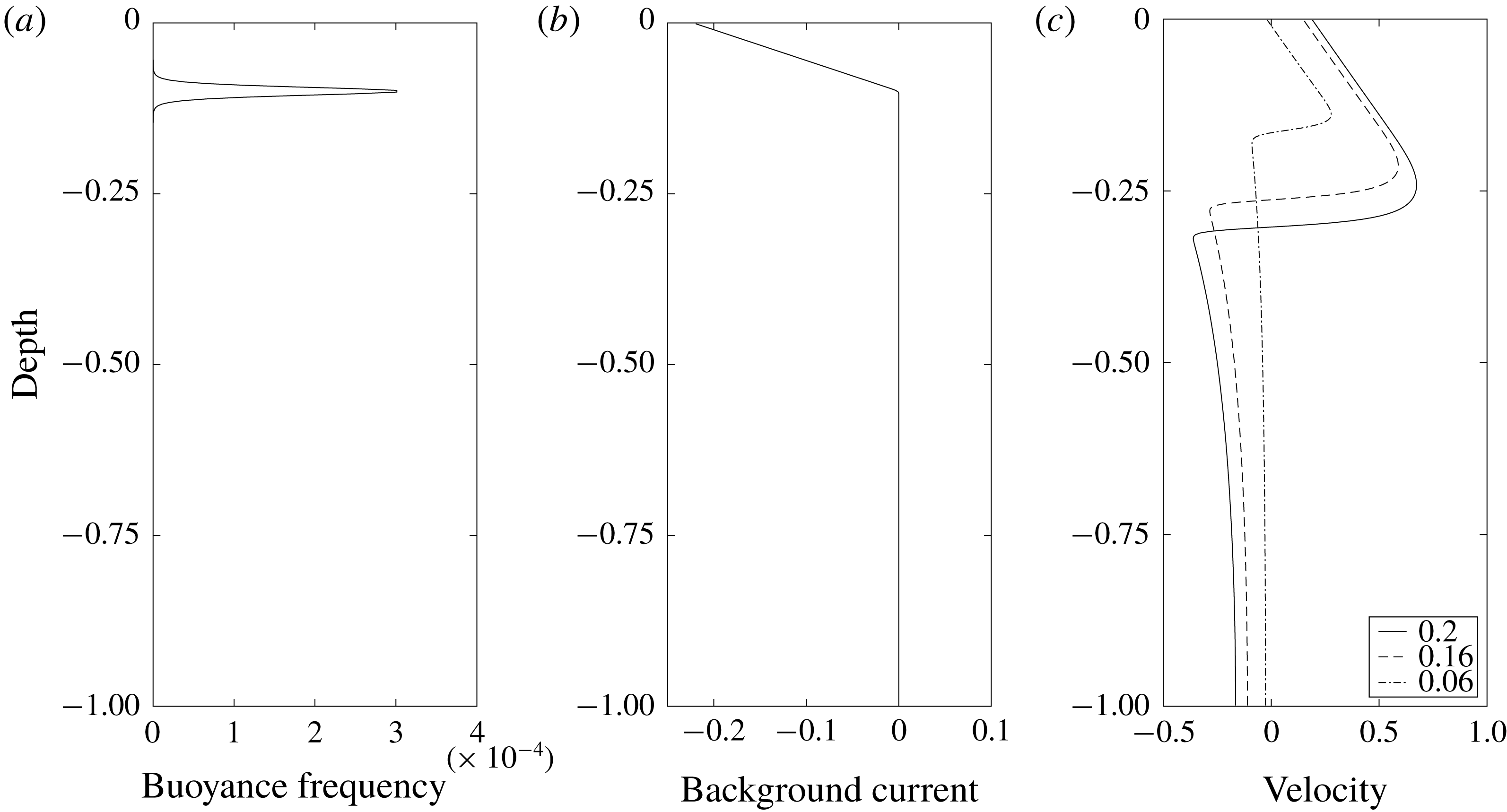
DJL solutions were computed to confirm our analytic solutions of the KdV theory. A more realistic, smoothed version of this two-layer configuration is used. Figure 10(a,b) shows the background buoyancy frequency and current profiles. Figure 10(c) shows the horizontal current profile down the centre of three different waves. In the upper layer with near-negligible baroclinic vorticity generation
 $u_{z}$
is approximately constant and negative, approximately equal to the vorticity of the background current. Across the thin pycnocline there is strong baroclinic vorticity generation resulting in large positive
 $u_{z}$
. Below the pycnocline
 $u_{z}$
is very small. Note that it is the vorticity
 $u_{z}-w_{x}$
which is zero in the lower layer and because of the finite length of the wave,
 $w_{x}$
, and hence
 $u_{z}$
, is not exactly zero in the lower layer or equal to the background vorticity in the upper layer. As the wave amplitude increases both
 $U_{sur}$
and
 $U_{max}$
increase with the latter increasing more rapidly, which confirms the pattern we observed in the KdV solutions. Background currents with positive near-surface vorticity can be analysed in a similar manner.
A simple two-layer model. (a) Stratification. (b) Model current. (c) Horizontal velocity down the centre of the waves with amplitudes of 0.2 (solid), 0.16 (dashed) and 0.06 (dash-dotted), respectively.
4 Numerical simulation of shoaling waves: comparison with observations
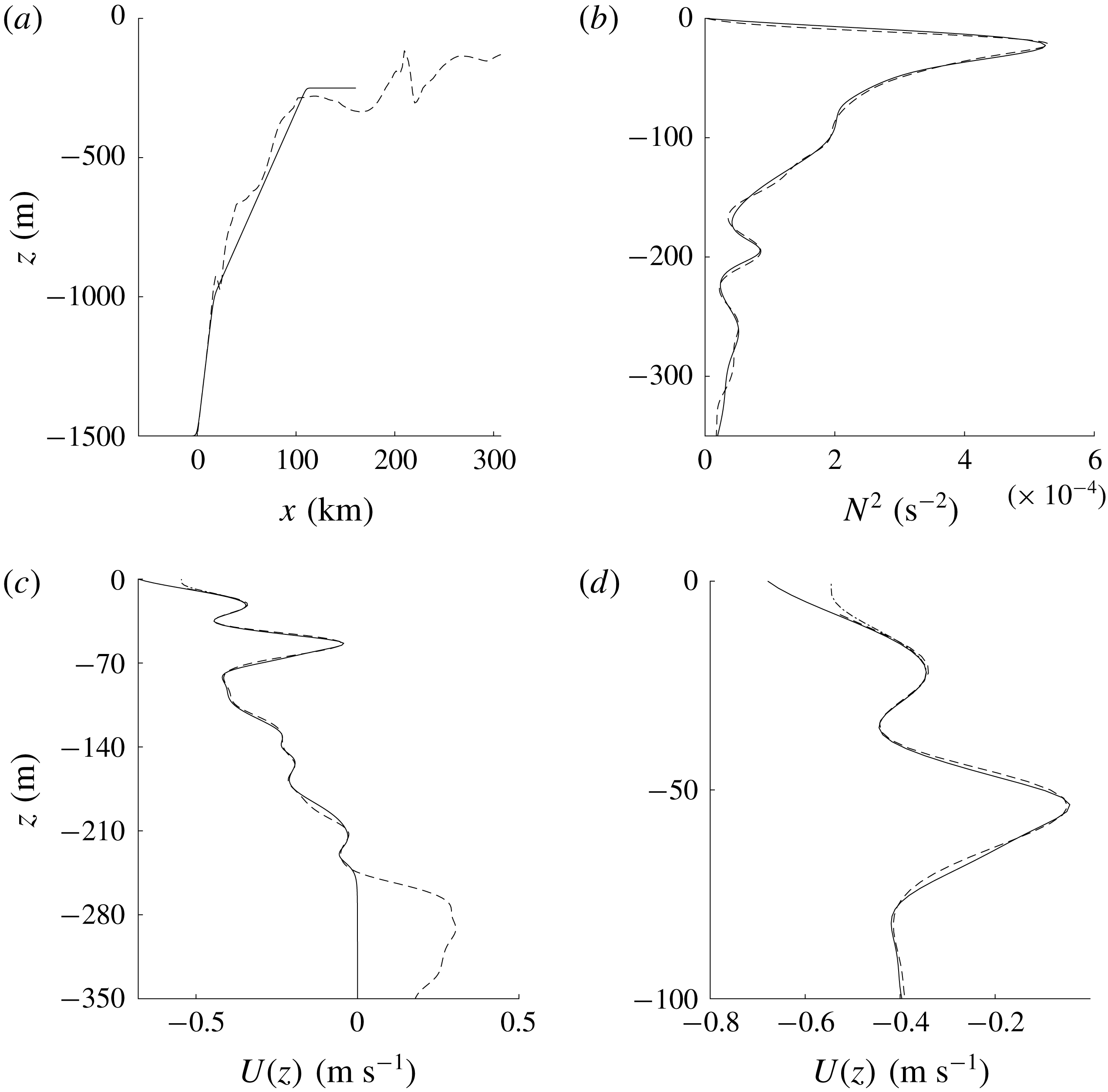
We now present a numerical simulation of a two-dimensional ISW shoaling over an idealized two-slope bathymetry (figure 11
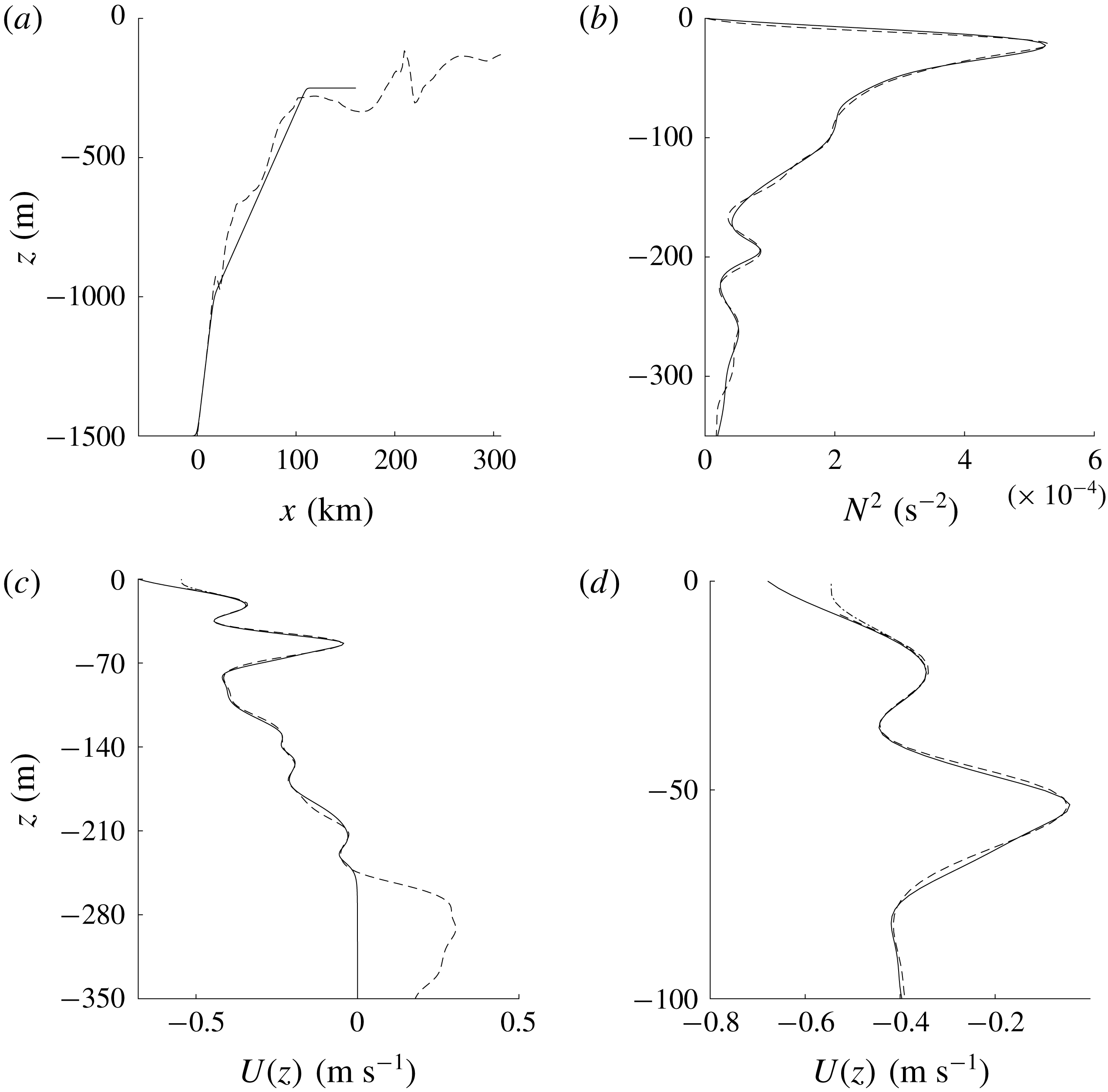
a). The wave observed in Lien et al. (Reference Lien, Henyey, Ma and Yang2014) propagated from deep water of approximately 3000 m depth onto the slope. We assume the bathymetry in the deep water region has a minor effect on the formation of waves with cores via shoaling. The slopes of the bathymetry used in our simulation was fitted to the upper part of the observed slope. The deep and shallow water depths are 1500 and 250 m. The Coriolis frequency
 $f=5.2\times 10^{-5}~\text{s}^{-1}$
is based on the observation location. The stratification profile used here (figure 11
b) is a better fit to the 2 June observation than the base profile in § 3. As the background current was not measured near the surface the current profile used in this simulation (figure 11
c) has been extrapolated to the surface in two ways,
 $(Ub_{neg})$
with negative and
 $(Ub_{0})$
with zero near-surface vorticity. Results for these two background currents were similar so only results from
 $Ub_{neg}$
are discussed here. The currents were rapidly brought to zero below 250 m depth so that it is zero below the top of the shelf. The initial ISW is a DJL solution with an amplitude of 183 m which is close to forming a core. The horizontal resolution was 10 m. The vertical resolution was varied from 3 to 0.5 m depending on the water depth.
Bathymetry, stratification and background current profiles. The black dashed lines are the observation data from 2 June (Lien et al.
Reference Lien, Henyey, Ma and Yang2014). In (a,b), the black solid lines are the profiles used in the shoaling wave simulations. (c) The two current profiles
 $Ub_{neg}$
(solid) and
 $Ub_{0}$
(dash-dot) used in the shoaling simulations. (d) Background currents in the upper 100 m.
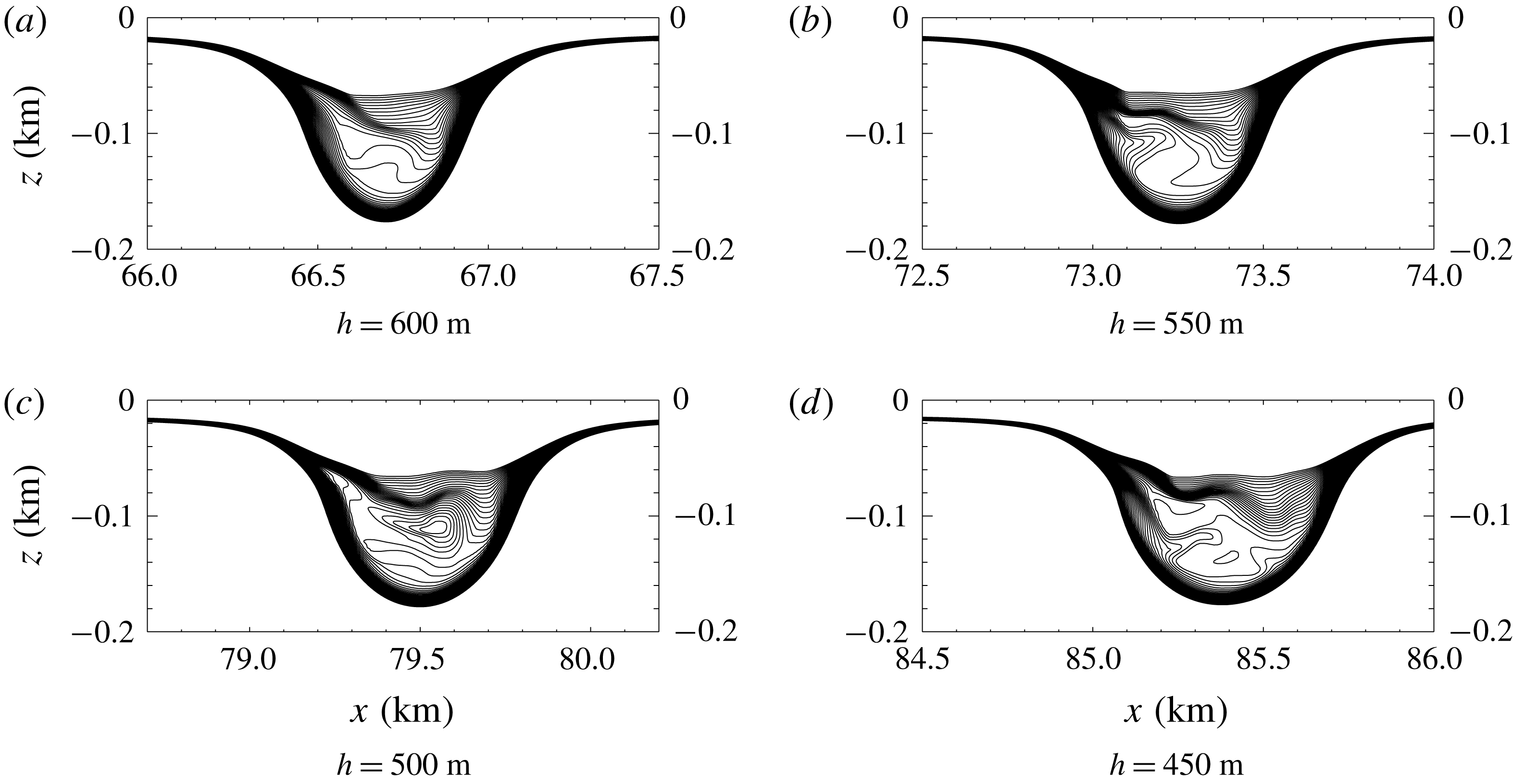
During the early stages of shoaling, the wave propagation speed decreases. The solitary wave gradually changes shape and a small, dispersive wave train is formed behind it. These are common features among shoaling waves. The density contours at depths
 $h=600$
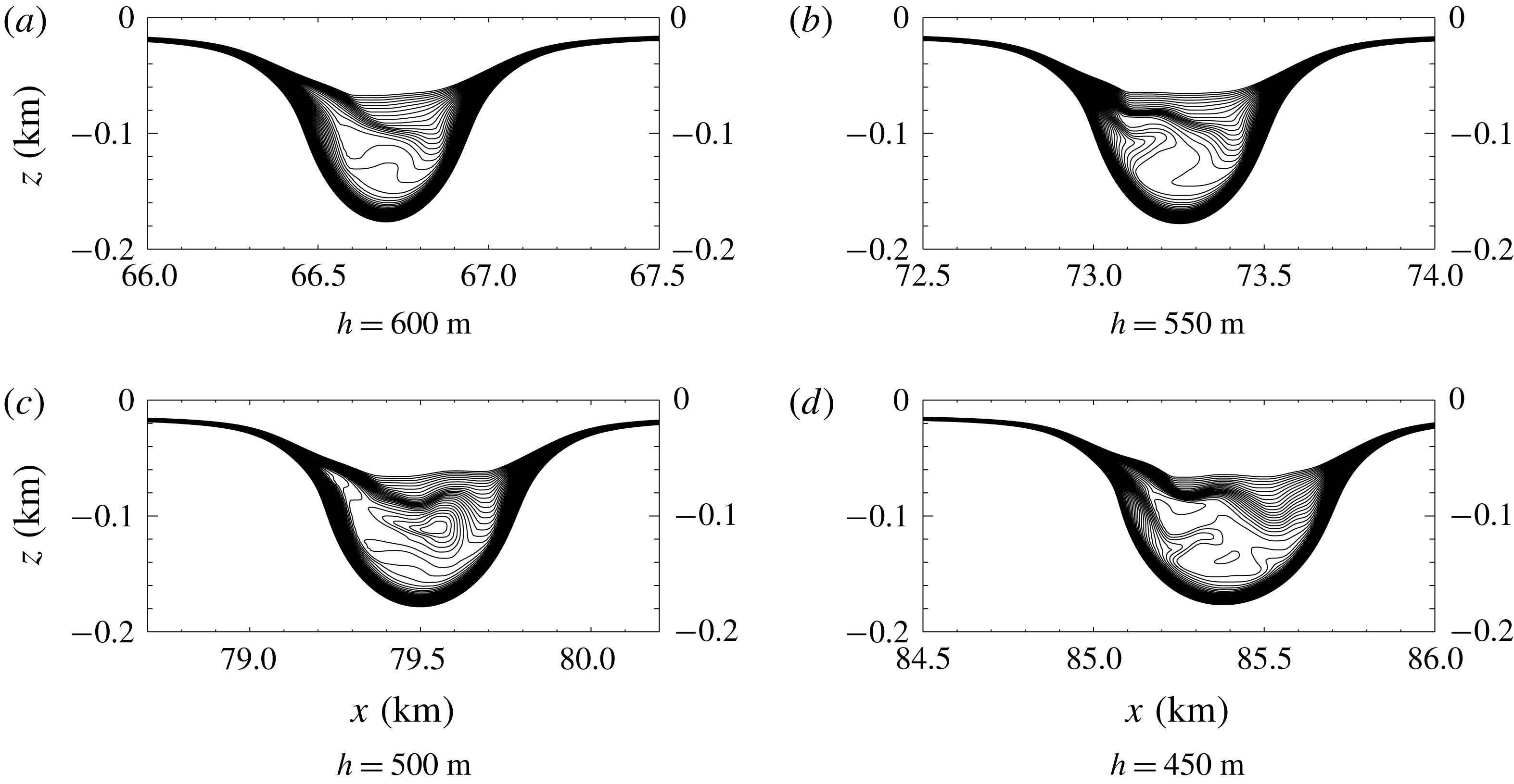
, 550, 500 and 450 m are shown in figure 12. Immediately after the density overturns, the fluid from the back of the wave plunges forward into the centre of the wave, forming a recirculating trapped core. The density in the core was denser than the surrounding fluid, which led to the mixing afterwards. The core structures in figure 12(c,d) are different illustrating the unsteady nature of the trapped core. The leading wave carried the core for a long distance while propagating onto the slope. Since the persistence of the core is not the focus of this paper, no plots of later stages are shown. In the ocean or laboratory experiments, the longevity of such cores would likely depend on three-dimensional effects and the intensity and evolution of turbulence inside the core. In this context we note that in simulations of internal wave boluses propagating on a shelf in a linearly stratified fluid (Venayagamoorthy & Fringer Reference Venayagamoorthy and Fringer2007) found that the dynamics of boluses in two-dimensional and three-dimensional simulations were very similar although their Reynolds numbers were well below field values.
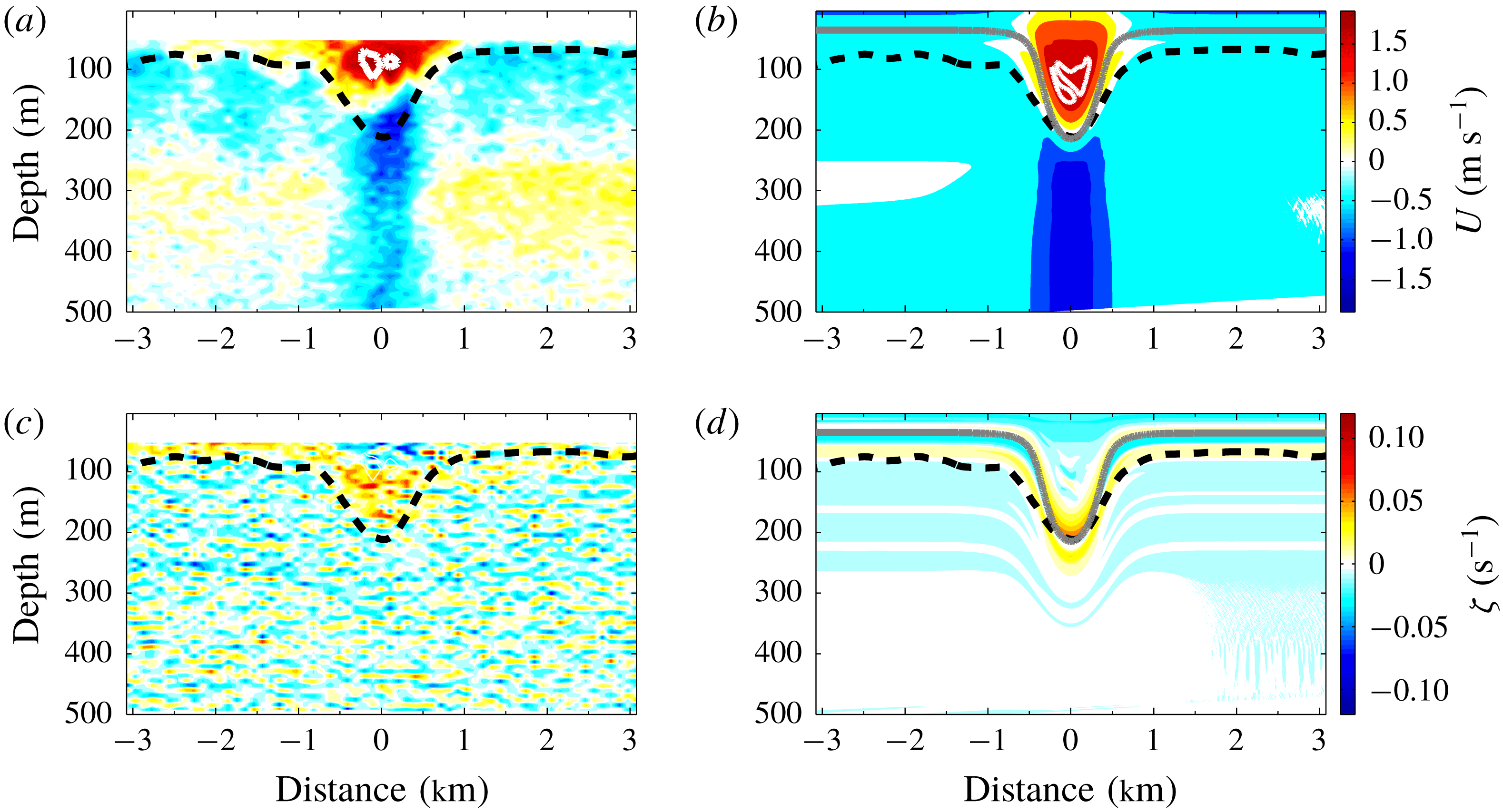
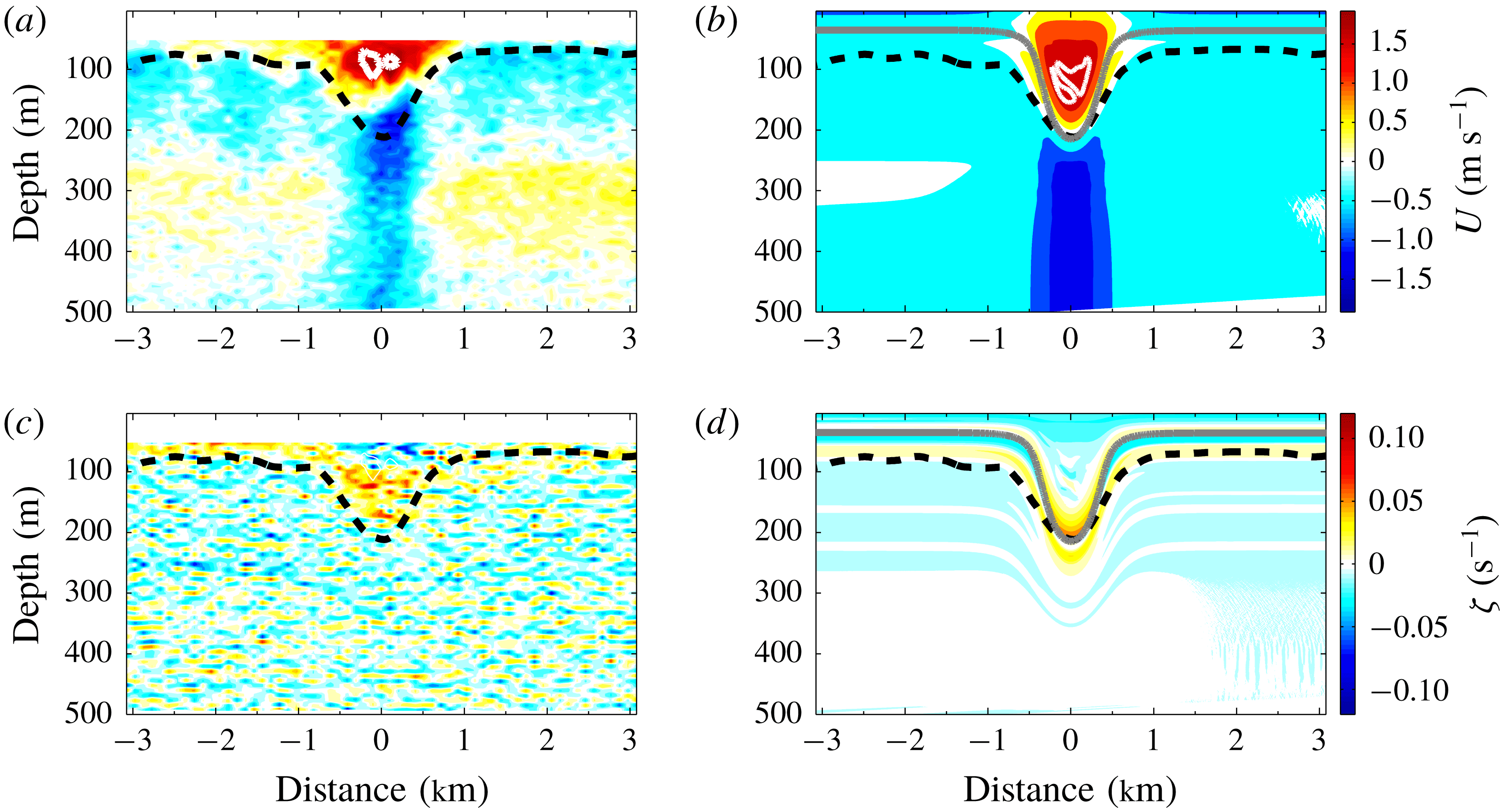
Comparisons of the vorticity and horizontal velocity in the numerical simulation and an observed wave are shown in figure 13. Overall the simulation is in good agreement with the observation. Both waves have a SSC, are nearly symmetric at this water depth and the horizontal velocities have the same order of magnitude. There are two major differences. In comparison with the observation, in the numerical simulation the core is at a greater depth and the rest height of the isopycnal undergoing the maximum vertical displacement is higher in the water column. The exact reasons for these differences are unknown but could be due to uncertainties in the near-surface background currents.
A close look at the formation of the shoaling wave with a trapped core. Here
 $h$
in the sub captions is the water depth representing the location of the leading solitary wave.
Comparisons between the observation (a,c) and the numerical simulation (b,d) at
 $h=450~\text{m}$
are plotted. The horizontal velocity and the vorticity contours are shown in the upper and the lower panels, respectively. The black dashed lines (observation) and the grey lines (simulation) are isopycnals undergoing the maximum vertical displacement. The thick white lines in the centre of the wave represent
 $u=c$
. Here the wave is propagating at
 $c=1.5~\text{m}~\text{s}^{-1}$
.
5 Summary
We have explored the conditions under which subsurface cores in ISW may exist by using solutions of the DJL equation to predict amplitudes at which the maximum current
 $U_{max}$
is equal to the wave propagation speed
 $c$
. This work was motivated by observations of ISW with SSCs in the South China Sea (Lien et al.
Reference Lien, Henyey, Ma and Yang2014) and we used a simple stratification fitted to the 2 June observations by Lien et al. (Reference Lien, Henyey, Ma and Yang2014) and a variety of background currents also motivated by these observations. We explored a simple case with no subsurface jet (
 $U_{m}=0$
). We later presented results from a two-dimensional numerical simulation of a shoaling ISW, using background conditions based on the observed conditions, which illustrated the formation of an ISW with a SSC.
The sign of the background current near-surface vorticity largely determines the location of the core. In particular, SC are formed when the near-surface vorticity of the background current is of the same sign as the wave induced vorticity, while SSC are formed when the signs are opposite. This difference occurs because, for the stratification used here, near-surface baroclinic generation of vorticity is weak and hence the vorticity of the background current is preserved in the centre of the wave above the pycnocline. If the stratification is strong up to the surface the baroclinic generation of vorticity could change this result. This criteria for the occurrence of SSCs is in agreement with the earlier findings of Choi (Reference Choi2006) in a two-layer fluid, each with constant vorticity, using a fully-nonlinear long wave two-layer model.
In general, it is easier to form a core as the magnitude of the current vorticity increases. However, since SSC are located lower than the SC, the generation of SSC is more sensitive to the magnitude of the current vorticity and the location of the pycnocline than SC are.
Our numerical simulation of a shoaling ISW does predict the formation of a SSC as observed in the South China Sea with some differences in the detailed structure of the wave. Possible explanations include differences in the bathymetry, stratification and background current profiles. A particular problem is the lack of observations of the background current within a few metres of the surface as the formation of the core is sensitive to the background conditions in this region.