1. Introduction

In the sea-ice modelling community, it is customary that ice melt is calculated both at the ice surface and bottom, but in many models ice growth is only considered at the ice bottom. in the melt season, however, formation of superimposed ice can take place via refreezing of surface snowmelt or rain (Reference KawamuraKawamura and others, 2001; Reference Granskog, Leppäranta, Kawamura, Ehn and ShirasawaGranskog and others, 2004, Reference Granskog, Vihma, Pirazzini and Cheng2006). Reference Granskog, Leppäranta, Kawamura, Ehn and ShirasawaGranskog and others (2004) suggested that superimposed ice could contribute up to 20% of the total ice mass during a winter season in the baltic sea. the modelling study by Reference Cheng, Launiainen and VihmaCheng and others (2003) suggested that, during the period when the ice is neither growing from the bottom nor melting, the formation of superimposed ice, rather than formation of snow ice due to ocean flooding, controls the total ice mass balance in the baltic sea. the two modelling periods were, however, too short (7 and 18 days) to draw firm conclusions, and a need for observations covering the entire snowmelt period became evident.

In march–april 2004, an ice station was set up on landfast sea ice in the gulf of bothnia, baltic sea. during the 4 week period, the entire snow layer, originally 0.15 ±0.05 m thick, was transformed to 7 cm of superimposed ice, except for 2 cm of snow that sublimated. an analysis of this process and its forcing conditions is given in Reference Granskog, Vihma, Pirazzini and ChengGranskog and others (2006), while Reference PerovichPirazzini and others (2006) present a detailed analysis on the observed snow/ice albedo. in this paper, we focus on numerical modelling of the superimposed ice formation. observations of the meteorological conditions and radiative fluxes at the ice station are used for forcing the thermodynamic snow/ice model of Reference Cheng, Launiainen and VihmaCheng and others (2003), while observations of the snow and ice evolution are used for the model initial conditions and validation, the latter being the basic motivation of this work.

We pay special attention to the factors critical for successful modelling of this snowmelt period. these include (a) the accuracy of the model forcing (sensitivity of the results to the differences between observed and parameterized radiative fluxes), (b) the processes inside the ice and snow (heat conduction, absorption of solar radiation, subsurface melting, and refreezing of meltwater) and (c) parameterization of the surface albedo. most parameterizations of the sea-ice albedo have been based on data from the arctic (Reference Flato and BrownFlato and brown, 1996; Reference Nicolaus, Haas, Bareiss and WillmesPerovich, 1996; Reference J.A., Schramm, Perovich and PintoCurry and others, 2001). because of the milder climate and generally thinner ice, the applicability of these parameterizations for the baltic sea ice cover is not well known.

2. Observations

Meteorological and glaciological observations were made on initially 0.55 ±0.03 m thick landfast sea ice in the gulf of bothnia, in the vicinity of the umeå marine sciences centre (umsc), sweden, at 63.57˚ n, 19.85˚ e (Reference Granskog, Vihma, Pirazzini and ChengGranskog and others, 2006). the study period lasted from 16 march (julian day 76; hereafter simply ‘day 76’) to 10 april (day 101) 2004. a meteorological station was installed on the ice, and air temperature (T _a) and relative humidity (rh), as well as wind speed (v _a) and direction at 2 m height were recorded. the downward (Q _s) and reflected (Q _r) shortwave radiation were measured with upward- and downward-facing eppley psp pyranometers. the downward and upward longwave fluxes (Q _d and Q _b, respectively) were measured with upward- and downward-facing eppley pir pyrgeometers. the surface albedo was solved from Q _s and Q _r, and the surface temperature (T _sfc) was solved from Q _b and Q _d (Reference PerovichPirazzini and others, 2006).

All data were sampled every minute and further averaged over 10 min. daily recordings of total precipitation were obtained from a precipitation gauge installed on the ice. cloudiness (C) was recorded by the same person at least every second hour during daytime (usually 0600–2000 h) throughout the whole period. observations of the air temperature, precipitation, radiative fluxes and the surface albedo are shown in figure 1.

Fig. 1.

(a–c) Time series of (a) air temperature (black line), surface temperature (grey line) and precipitation (bars); (b) observed (grey dots) and parameterized (solid line) downward shortwave radiation; and (c) observed (grey dots) and parameterized (solid line) downward longwave radiation. (d) Observed (grey dots) and (e) calculated (solid line) surface albedo. In the calculation of albedo (Reference Flato and BrownFlato and Brown, 1996), the modelled surface temperature is used in (d), while the observed surface temperature is used in (e).

The glaciological observations included collection of ice cores at about 1–3 day intervals, and measurements of the snow and ice thickness and ice freeboard. in addition, at weekly intervals (days 79, 86, 93 and 101) ten ice cores with a horizontal spacing of 1 m were collected along a representative line. consecutive horizontal lines were spaced 1 m apart. along each line, snow and ice thickness and ice freeboard were recorded. we use the latter data for model validation, as they better represent spatial averages. the temporal resolution of these data was, however, not sufficient in the beginning of the experiment, when heavy snowfall occurred. hence, the initial snow and ice thickness applied in the model are based on the first individual measurements.

The thickness of the surface granular ice layer was determined on the basis of the crystal texture in the ice cores. results of the salinity and stable-isotopic analysis indicated that all the granular ice was superimposed ice (Reference Granskog, Vihma, Pirazzini and ChengGranskog and others, 2006). snow density and temperature were occasionally measured and used for model initialization and validation.

3. Thermodynamic SNOW/ICE Model

A one-dimensional high-resolution thermodynamic snow/ice model developed by Reference Launiainen and ChengLauniainen and Reference ChengCheng (1998) and Reference Cheng, Launiainen and VihmaCheng and others (2003) was used in this study. the model is similar to Reference Liston, Winther, Bruland, Elvehøy and SandMaykut and untersteiner (1971), but the penetration of solar radiation in snow and ice is parameterized in more detail. in addition, the mechanisms of superimposed ice and snow-ice formation are taken into account. the basic model equations are:

(1)

(2)

(3)

(4(a))

(4(b))

(4(c))

(5)

The heat conduction in snow and ice is solved from equation (1), where T is the temperature, ρ is density, c is specific heat, k is thermal conductivity and q(z,t) is the amount of solar radiation penetrating below the surface (in the equations, z is positive downwards). subscripts s and i denote snow and ice, respectively.

The surface heat- and mass-balance equation (2) is the upper flux boundary condition of equation (1). the solar radiation Q _s is parameterized by the scheme of Reference SalorantaShine (1984) combined with the cloud effect of Reference LaevastuLaevastu (1960). the longwave fluxes Q _d and Q _b are calculated by the formula of Reference Pirazzini, Vihma, Granskog and ChengPrata (1996) with the cloud effect of Reference Jacobs, Barry and JacobsJacobs (1978). ε is the surface emissivity (0.97). the turbulent fluxes of sensible heat Q _h and latent heat Q _le are calculated by applying the bulk method, where the observations of the wind speed, air and surface temperature and air relative humidity are used. F _c is the surface conductive heat flux.

I ₀ is the portion of solar radiation penetrating below the surface layer and contributing to internal heating of the snow/ice. the term (1–α _s,i)Q _s –I ₀ represents the shortwave radiation contributing to the surface heat balance. α is the surface albedo (see section 4 for its parameterization). the surface temperature T _sfc is solved from equation (2). when T _sfc tends to be above the freezing temperature (T _f), T _sfc remains at T _f and the excessive heat (F _m) is used for melting: dh _s,i /dt = F _m/ρ _s,i L _f, where h _s,i is the thickness of snow or ice and L _f is the latent heat of fusion. all fluxes are defined positive to the surface.

equation (3) is the mass balance at the ice bottom, where F _w is the oceanic heat flux (assumed to be constant) and the ice bottom temperature (T _bot) remains at the freezing temperature of sea water.

Equations (4a–4c) present the penetrating solar radiation in snow and ice; the bouguer–lambert law is applied. к is the extinction coefficient. for snow, к _s varies from 15 m^–1 for old snow up to 25 m^–1 for new snow. for sea ice, however, the penetrating solar radiation is considered separately for the uppermost 10cm of ice and the layers below. i ₀ is the bulk fraction of the incident irradiance transmitted through the uppermost 0.1 m in sea ice (e.g. i ₀ = 0.18(1 –C) + 0.35C for white ice, and i ₀ = 0.43(1 – C) + 0.63C for blue ice (Reference Grenfell and MaykutGrenfell and maykut, 1977; Reference Nicolaus, Haas, Bareiss and WillmesPerovich, 1996)). because there is exponential decay of penetrating solar radiation from the uppermost layer of snow/ice, the magnitude of solar radiation contributing to the surface heat balance ((1–α _s,i)Q _s–I ₀) depends on the thickness of the model surface layer. this model differs from most previous models, which have a thicker (>10 cm) surface layer. a more sophisticated method to calculate the penetration of solar radiation would be a radiative transfer scheme (e.g. Reference Launiainen, Cheng, Uotila and VihmaListon and others, 1999). our comparison (Reference ChengCheng, 2002) showed, however, that the results based on the bouguer–lambert law were close to the results of Reference Launiainen, Cheng, Uotila and VihmaListon and others (1999), in particular for snow.

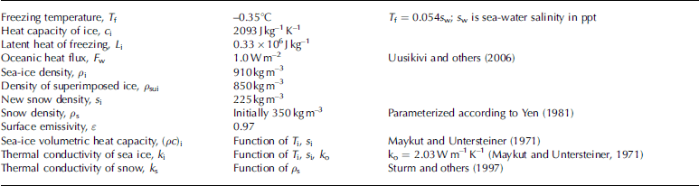
equation (5) is the mass balance at the snow/ice interface; if meltwater is present, the heat-flux divergence at the interface results in an increase in the superimposed ice thickness (H _sui). after superimposed ice is formed, it becomes an integral part of the total ice thickness. the factors controlling the snow evolution are precipitation, snowmelt, refreezing, snow compaction (Reference J., Ehn and GranskogYen, 1981) and slush formation resulting from water flooding (Reference PrataSaloranta, 2000). the model parameters are summarized in table 1.

Table 1.

Model parameters and constants based on observations and literature

In order to reproduce the exponential decay of penetrating solar radiation in snow and ice, high vertical resolution in a lagrangian grid mode with 10 layers in the snow and 20 layers in the ice is used. this is critical both under conditions of large solar radiation and during rapid temperature changes (Reference ChengCheng, 2002).

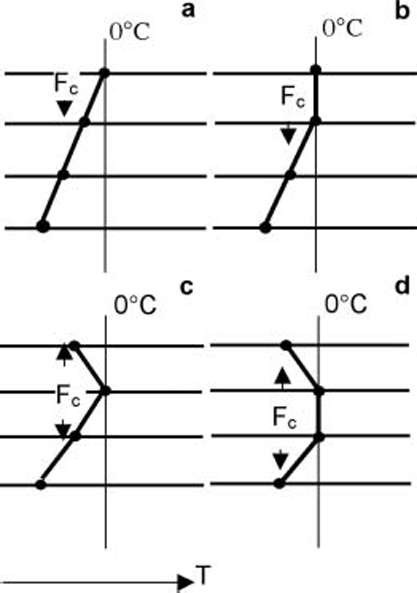
figure 2 illustrates the possible forms of the modelled snow/ice temperature profile during melting. if there is snow on the ice, meltwater is assumed to have no heat exchange with the surrounding snow and to percolate down to the snow/ice interface without time delay, i.e. the time required for the percolation is assumed to be much shorter than the time of the refreezing. this is supported by recent findings: it was observed in the weddell sea in austral summer 2005 that the percolation time for a tracer through a 40 cm thick snow layer was only about 6 hours (personal communication from c. haas, 2005). similar results were obtained in hudson bay, canada, in summer 2005 (granskog, unpublished information). when the interface has below-zero temperatures, the refreezing and release of latent heat are first calculated, and the heat conduction is calculated thereafter.

Fig. 2.

Temperature profiles for various melting conditions in a high-resolution model: (a) surface temperature at the melting point; (b) melting of a surface layer consisting of at least two model levels; (c) subsurface melting at a single model level; and (d) subsurface melting in a layer consisting of at least two model levels.

4. Model Experiments and Results

Two strategies were applied to find the most critical factors for successful modelling of snow and sea-ice thermodynamics during this spring period: (a) forcing the model with parameterized air–ice fluxes, and (b) prescribing the air–ice fluxes according to the observations. in a the surface temperature is computed in the model, whereas in b it is prescribed on the basis of the longwave radiation measurements. approach a corresponds to the normal situation in modelling applications, except that now our information on the air temperature, humidity, wind speed and cloud fraction is based on direct observations, while in operational and climate modelling applications this information is based on the output of an atmospheric model. the parameterized surface fluxes do, however, include errors in a; these, together with the errors in modelling the thermodynamic processes inside the ice and snow, contribute to model errors. in b, basically only the errors related to the modelling of processes inside the ice and snow are present. in addition, there are inaccuracies in the observed surface fluxes, but these are much smaller than errors in the parameterized fluxes in a. in both strategies, we also study the sensitivity of the results to the snow/ice surface albedo.

A: simulations with parameterized atmospheric forcing

We made three model simulations. we first discuss the model results when the surface albedo was prescribed according to the observations; we refer to this as the reference run (a_REF). the turbulent and radiative fluxes were parameterized as presented in the model description. the parameterized radiative fluxes are plotted in figure 1b and c, together with observed values. the incoming shortwave and longwave radiation had mean biases of –10 and 19wm^–2, respectively. the turbulent fluxes were typically much smaller in magnitude than the radiative fluxes, and their absolute errors were therefore smaller. on the basis of our previous validations (Reference Launiainen, Cheng, Uotila and VihmaLauniainen and others, 2001), the accuracy of the parameterized turbulent fluxes is of the order of ±20%, which in this case typically corresponds to an error less than ±5wm^–2.

The observed and modelled snow temperature profiles are shown in figure 3. in the morning, the snow temperature profile indicated upward heat conduction, while in the afternoon most of the snow layer was in an isothermal melting phase, the result of penetration of solar radiation. these features were well reproduced by the model. on day 79 at 0700 h, the model error is mostly due to the error in the modelled snow surface temperature (also associated with error in snow thickness). the warming of the uppermost snow layers, observed at 0925 h, was delayed in the model, which suggests inaccuracies in the modelled snow properties.

Fig. 3.

The observed (symbols) and modelled (A_REF; lines) snow temperature profiles on (a) day 79 and (b) day 88. The zero depth refers to the snow/ice interface. The observed surface temperature at 0700 h on day 79 was measured by a hand-held temperature probe (Testo 720), while the other surface temperatures were derived from the observed longwave radiation.

Time series of the modelled snow thickness and the depth of the melt layer are shown in figure 4. until day 82, the melting took place roughly in the uppermost 6–7cm of the snowpack, i.e. in a layer thicker than the model surface layer. during the colder period on days 83–86, no surface melting was modelled, but the solar radiation caused subsurface melting, which is in agreement with observations (figure 6a indicates no surface melting, but figure 5c indicates growth of superimposed ice). the subsurface melting took place in more than one model level, i.e. on days 83–86 the situation in figure 4was as in figure 2d.

Fig. 4.

The time series of modelled (A_REF) snow thickness. The white area below the surface indicates the region of active melt in the snow.

Fig. 5.

Observed and modelled evolution of (a) snow thickness H _s, (b) ice freeboard, (c) superimposed ice thickness H _sui and (d) total ice thickness H _i. The observations are marked by circles, with the vertical bar indicating the spatial standard deviation (n = 10). The solid lines indicate model results of A_REF, while the dotted and dashed lines indicate model results of A_P and A_FB, respectively.

Fig. 6.

Time series of the surface temperature: (a) observations (grey dots) and results of A_REF (solid line); (b–d) errors in A_REF (b), A_P (c) and A_FB (d).

A comparison of the time series of the observed and modelled snow thickness, ice freeboard, superimposed ice thickness and total ice thickness is shown in figure 5. the snowfall on days 77–81 was associated with snowmelting, and the snow thickness did not change much before day 86. the early difference between observed and modelled snow thickness probably resulted from spatial variability and inaccuracy in the density of newly fallen snow. the model reproduced the major snowmelt event (days 86–93) with a slight overestimation of total melt and advance of the final disappearance of the snow. the latent-heat flux calculated on the basis of the meteorological observations suggested that a total of 0.9 cmw.e. of snow sublimated during the observation period, and the modelled total sublimation was 0.8 cm. because of a realistic simulation of the snow load, the ice freeboard was also properly reproduced (fig. 5b).

Observations showed that the thickness of the superimposed ice on top of the ice layer increased substantially (fig. 5c). the total modelled superimposed ice growth was 10 cm, while the observed value was 9.5 cm. due to the intermediate decrease of superimposed ice thickness from day 88 to 90, the observed net growth was, however, only about 7 cm. the observed total ice growth almost equalled the superimposed ice growth on the ice surface, and this was also the case in modelling (fig. 5d). the study period was in spring, and the initial ice thickness was >0.5 m. hence, a very cold surface would have been needed for significant formation of new ice at the ice bottom. under current forcing conditions, instead of bottom freezing, slight bottom melting was calculated (0.7 cm).

In table 2 we present quantitative results for the observed and modelled changes in the snow, superimposed ice and ice thickness. we divide the period into three parts: days 80–86 (steady increase in H _sui), days 87–89 (cycle of melting and refreezing) and days 90–101 (rapid growth followed by quasi-steady state).

Table 2.

Observed and modelled (model runs A_REF, A_P, A_FB, B_REF and B_FB) variation of snow, superimposed ice and total ice thickness (in cm) in three periods: days 80–86, 87–89 and 90–101

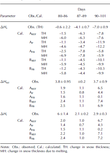
From day 80 to 86, the model underestimated superimposed ice growth. daytime melting was seen in deep layers in the snowpack (fig. 4), and there would have been enough water available to form as much superimposed ice as observed. at the snow/ice interface, however, the heat-flux divergence was not large enough for refreezing of all the meltwater (table 2: in a_REF, 6cm of snow was melted, but only 1.9cm of superimposed ice was generated). in the model, refreezing is calculated only at the snow/ice interface, but in reality part of the refreezing had already occurred in the intermediate layers and it was often hard to distinguish the exact transition from snow to superimposed ice (Reference Granskog, Vihma, Pirazzini and ChengGranskog and other, 2006).

During days 87–89, the modelled melting took place only in the snow layer, and the observed decrease of H _sui was therefore not reproduced (fig. 5c). this is perhaps due to the simplification of snow processes. the model produced reasonable results for the superimposed ice thickness from day 90 to 101. the snow temperature had a large diurnal cycle, which strongly attenuated with depth in the snowpack. this, and the fact that the snow cover was now thinner than during days 80–86, helped to generate a heat-flux divergence large enough to refreeze almost all the meltwater (7.6cm in snow thickness; table 2). the overestimation of superimposed ice formation during this period (fig. 5) could be due to the refreezing of the meltwater from the previous periods (days 80–89).

Two sensitivity tests focusing on the snow/ice albedo were made. in the first test, referred to as A_P, the albedo was parameterized according to the status of the surface: 0.8 for snow, 0.77 for wet snow, 0.7 for ice and 0.3 for wet ice (Reference Nicolaus, Haas, Bareiss and WillmesPerovich, 1996). in the second test, referred to as A_FB, the albedo was calculated according to Reference Flato and BrownFlato and brown (1996), hereafter fb. the parameterization of fb takes into account the effects of snow and ice thickness as well as surface temperature, which affects snow metamorphism and melting. in fb, the use of two formulas depending on the T _sfc results in a strongly fluctuating albedo time series (fb developed the scheme on the basis of daily mean values, but in our data the diurnal cycle is large).

In A_P, with no direct albedo dependence on T _sfc, the snow thickness was overestimated but the total snowmelt was reasonably reproduced (fig. 5a). the slower increase of H _sui compared with A_REF (fig. 5c) was due to a relatively weak heat-flux divergence at the snow/ice interface due to the overestimated snow depth from day 90 to 101. in A_FB, with the albedo depending on T _sfc, the calculated albedo decreased rapidly in days 87–90 (fig. 1d). due to the strong positive feedback between the albedo and surface temperature, which is presented in fb, the model produced rapid snowmelt until the snow totally disappeared well in advance of the observed disappearance, A_REF, and A_P. the errors in the modelled T _sfc mostly resulted from the overestimation of the downward longwave radiation (fig. 1c). on the other hand, if a modified version of the fb parameterization (Reference PerovichPirazzini and others, 2006; tuned on the basis of our data) was used, the results were almost identical to those in the reference run.

The observed and modelled time series of the surface temperature are shown in figure 6. it is noteworthy that the error in T _sfc does not depend much on the surface albedo used in the model (cf. fig. 6b, c and d; the mean absolute errors are 0.2 k for A_REF, 0.3 k for A_P and 0.5 k for A_FB). this is because the largest errors (up to 5 k) occurred at night (fig. 6a). the daytime values agreed better because the melting temperature was often reached (but due to the strong albedo feedback in A_FB, even the smaller daytime errors in T _sfc generated errors in the absorbed solar radiation and mass balance, as reported above). the night-time errors were mostly due to the poor performance of the longwave radiation scheme (in conditions of T _sfc<–3˚c, the linear correlation coefficient between the errors in T _sfc and Q _d was 0.51). however, although smaller in magnitude, the probable errors in the turbulent sensible heat flux and the conductive heat flux in the ice and snow can contribute to the error in T _sfc.

B: simulations with observed surface temperature, albedo and radiative fluxes

We present a simulation B_REF with the surface temperature, albedo and radiative fluxes prescribed according to the observations. the results (fig. 7) only show the time series of snow thickness and superimposed ice thickness (ice freeboard is controlled by the snow thickness, and the ice mass balance by the superimposed ice growth). the evolution of the snow thickness from day 90 onwards is now better reproduced than in A_REF (cf. figs 5 and7), which suggests that the internal processes in the snow cover are reasonably well modelled.

Fig. 7.

Observed (circles) and modelled evolution of (a) snow thickness and (b) superimposed ice thickness. The solid lines indicate results of B_REF, while the dotted lines indicate results of B_FB.

Comparing figures 5 and 7, we conclude that the model results for the snow and ice mass balance are not sensitive to the large errors in surface temperature at night. the reason is that, when both observations and model results indicated freezing temperatures, as they did during most nights, the liquid water refroze (except on days 86–88) and even a 5 k error in the surface temperature did not affect the mass balance.

Finally, we present a sensitivity study B_FB with the surface temperature and surface fluxes prescribed according to the observations, as in B_REF, except that surface albedo is parameterized according to fb. in this case, the albedo affects (a) the surface melting by affecting F _m in equation (2), and (b) the subsurface melting due to penetration of solar radiation into the snow and ice. the results are, however, almost equal to those of B_REF with the prescribed albedo (fig. 7) due to the lack of feedback between the surface temperature and albedo (fig. 1e). the importance of the feedback is demonstrated by the large difference between the results of A_FB (fig. 5) and B_FB (fig. 7).

We see from table 2 that results for the mass balance were almost equal in B_REF and A_REF, which differed from each other only in the external forcing. results for A_FB and B_FB differed a lot from each other, particularly for superimposed and total ice thicknesses.

5. Conclusion

We have presented a modelling study on the snowmelt period in the baltic sea, when a 15 cm thick snow layer on the ice was transformed into a 7cm thick superimposed ice layer, except for 2 cm of snow sublimation. the high-resolution model performed well in simulating the surface energy budget, snowmelt and refreezing. the model, however, did not simulate all temporal variations in the superimposed ice thickness. the reasons may be linked to the uncertainties in snow properties and the model assumption of refreezing only at the snow/ice interface. on the other hand, the model yielded snow temperature profiles in good agreement with observations. we are not aware of any other modelling study on superimposed ice formation that covers the entire snowmelt period with detailed validation against observations.

We separated the direct effect of the inaccuracy in the snow/ice albedo from the surface temperature feedback effect. our calculations suggest that, if a reasonable albedo parameterization is applied, the direct effect of the inaccuracy in albedo is minor even in conditions of rapid snowmelt. on the other hand, large errors in the modelled ice and snow mass balance can be produced even with the surface albedo parameterized according to a sophisticated scheme (e.g. Reference Flato and BrownFlato and brown, 1996), which takes into account the effects of snow and ice thickness and surface temperature (cf. Reference J.A., Schramm, Perovich and PintoCurry and others, 2001). during the simulation, the errors grew rapidly due to the strong positive feedback effect related to a too strong effect of temperature on the albedo in the Reference Flato and BrownFlato and brown (1996) parameterization (Reference PerovichPirazzini and others, 2006).

Despite the important feedback mechanism between the surface temperature and albedo, the surface albedo did not significantly affect the accuracy of the modelled surface temperature. the errors in the surface temperature were almost equally large when the observed albedo and the albedos resulting from the two parameterizations were applied. this is because the maximum errors occurred at night and were mostly due to the errors in the net longwave radiation and turbulent fluxes in a stably stratified atmospheric boundary layer.

As in previous studies (Reference ChengCheng, 2002; cheng and others, 2002), high vertical resolution in snow and ice was a prerequisite for accurate simulation of subsurface melting; we used 10 layers in the snow and 20 in the ice. the results of this study suggested that, in further development of high-resolution thermodynamic snow and ice models for the baltic sea, high priority should be given to the parameterization of (1) surface albedo, (2) radiative fluxes, in which simple schemes may yield large errors, and (3) air–ice exchange during the night. in this study, the surface temperature errors were not critical for the ice and snow mass balance, but in slightly warmer conditions equally large errors could have been critical if the erroneous simulations had not yielded freezing temperatures at night. further, when a snow/ice scheme is applied in a numerical weather-prediction model, surface temperature errors can be critical for the forecasts for near-surface air temperature and fog formation.

In the polar oceans, the boundary conditions for snowmelt are somewhat different from those in the baltic sea. in the polar oceans, melting occurs mostly in late spring or summer, while in the baltic sea near-surface temperatures above 0˚c are reached in early spring and even in midwinter, during periods of warm-air advection from the atlantic ocean or central europe. the earlier melting season in the baltic sea is characterized by lower values of incoming solar radiation compared to the later melting in the polar oceans, and by the alternation of daylight and night, which can cause rapid freezing at night and melting in the daytime. the baltic sea has lower water salinity than the polar oceans, so the ice bottom temperatures are higher,

Which affects refreezing. for model applications in the polar oceans, the heat conduction inside the ice and the penetration of solar radiation may therefore be even more important processes than the results of this study suggest. however, important differences in snow thinning over sea ice during the melting season also exist between the arctic and antarctic (Reference Maykut and UntersteinerNicolaus and others, 2006).