


1 Introduction
Compliant wall technology originates from Gray’s paradox (Gray Reference Gray1936) concerning the apparent deficit between the muscle power of a dolphin and the power required by the dolphin to sustain its motion while swimming. Gray suggested that the skin of a dolphin may have anti-drag properties. One approach to drag reduction originated from Kramer (Reference Kramer1957, Reference Kramer1960, Reference Kramer1962) who proposed that compliant surfaces, such as dolphin skin, could reduce friction drag by delaying laminar–turbulent transition. Although the resulting research had mixed outcomes (Gad-el-Hak Reference Gad-el-Hak2002), Kramer’s hypothesis was proven through stability analysis (Carpenter & Garrad Reference Carpenter and Garrad1985, Reference Carpenter and Garrad1986; Davies & Carpenter Reference Davies and Carpenter1997a ,Reference Davies and Carpenter b ), experiments (Lee, Fisher & Schwarz Reference Lee, Fisher and Schwarz1993a ,Reference Lee, Fisher and Schwarz b , Reference Lee, Fisher and Schwarz1995), and direct numerical simulation (DNS) (Wang, Yeo & Khoo Reference Wang, Yeo and Khoo2005, Reference Wang, Yeo and Khoo2006). Recently, Bale et al. (Reference Bale, Hao, Bhalla, Patel and Patankar2014) pointed out that muscle power had to provide thrust, rather than exceed drag, highlighting a fundamental flaw in Gray’s hypothesis, confirmed also by Fish et al. (Reference Fish, Legac, Williams and Wei2014).
Compliant wall models: spring and damper supported membrane as an example of pressure-driven wall model with wall-normal deformation response (a); pressure- and wall-shear-stress-driven anisotropic coating model proposed by Fukagata et al. (Reference Fukagata, Kern, Chatelain, Koumoutsakos and Kasagi2008) (b). Wall displacement components are denoted by
 $\unicode[STIX]{x1D709}$
and Cartesian coordinates by
 $x_{i}$
.

Meanwhile, a second approach to drag reduction considered the turbulent boundary layer over a compliant surface (Bushnell, Hefner & Ash Reference Bushnell, Hefner and Ash1977). Theoretical studies, such as by Duncan (Reference Duncan1986) and Kireiko (Reference Kireiko1990), focused primarily on pressure-driven compliant surface models with wall-normal velocity response, as shown in figure 1(a). Using the same model with DNS, Xu, Rempfer & Lumley (Reference Xu, Rempfer and Lumley2003), Kim & Choi (Reference Kim and Choi2014) and Xia, Huang & Xu (Reference Xia, Huang and Xu2017) reported either increased friction drag or else a statistically unchanged flow field. These findings contradict theoretical predictions (Duncan Reference Duncan1986; Kireiko Reference Kireiko1990) and experimental results (Choi et al. Reference Choi, Yang, Clayton, Glover, Atlar, Semenov and Kulik1997) where 7 % drag reduction was measured on slender bodies coated with single-layer homogeneous viscoelastic material. Ongoing research, for instance, Rosti & Brandt (Reference Rosti and Brandt2017), Xia et al. (Reference Xia, Huang and Xu2017), Zhang et al. (Reference Zhang, Wang, Blake and Katz2017), is aimed at understanding the interaction between turbulent boundary layers and passive wall motions in the context of compliant wall design.
Common practice involves first identifying beneficial wall motions based on active flow control, and then developing and optimising a wall model that sustains favourable deformations. Endo & Himeno (Reference Endo and Himeno2002) and Xu et al. (Reference Xu, Rempfer and Lumley2003) applied the spring and damper supported membrane model in figure 1(a) to explore whether it could sustain the wall-normal opposition control proposed by Choi, Moin & Kim (Reference Choi, Moin and Kim1994). During opposition control, the wall-normal velocity of the surface is set equal in magnitude and opposite in direction to the fluctuating wall-normal fluid velocity component at a specified distance from the wall. Although Endo & Himeno (Reference Endo and Himeno2002) believed they measured a modest 2–3 % drag reduction, Xu et al. (Reference Xu, Rempfer and Lumley2003) found that this was a consequence of the short averaging time and concluded that pressure-driven compliant walls cannot sustain wall-normal opposition control. Fukagata et al. (Reference Fukagata, Kern, Chatelain, Koumoutsakos and Kasagi2008) examined a compliant wall deformed both by pressure and streamwise wall shear stress as shown in figure 1(b). This surface was designed to exploit the drag-reduction mechanism of an active control proposed by Fukagata & Kasagi (Reference Fukagata and Kasagi2004) where the wall-normal velocity was actuated according to streamwise wall shear stress. Fukagata et al. (Reference Fukagata, Kern, Chatelain, Koumoutsakos and Kasagi2008) utilised an evolutionary optimisation method that achieved 8 % drag reduction in a turbulent channel flow. However, the optimised coating led to a statistically unchanged flow field in a larger channel geometry.
Kim & Choi (Reference Kim and Choi2014) have investigated whether favourable wall-normal deformations exhibiting streamwise travelling waves, first observed by Nakanishi, Mamori & Fukagata (Reference Nakanishi, Mamori and Fukagata2012), can exist on a viscoelastic coating using the model depicted in figure 1(a). For soft coatings Kim & Choi (Reference Kim and Choi2014) found that when pressure-induced travelling waves on the coating surface have favourable convection velocity, the wave amplitude is too high. Such large-amplitude waves result in a roughness effect, leading to drag increase on the channel walls. Kim & Choi (Reference Kim and Choi2014) concluded that stiff coatings sustaining small-amplitude deformations cannot significantly modify the turbulent flow. These findings may explain why recent numerical studies consistently report either an increase in drag or a statistically unchanged flow field in the presence of travelling wave-like wall deformations (Xu et al. Reference Xu, Rempfer and Lumley2003; Fukagata et al. Reference Fukagata, Kern, Chatelain, Koumoutsakos and Kasagi2008; Rosti & Brandt Reference Rosti and Brandt2017; Xia et al. Reference Xia, Huang and Xu2017). More recently, Zhang, Miorini & Katz (Reference Zhang, Miorini and Katz2015), Zhang et al. (Reference Zhang, Wang, Blake and Katz2017) have reported pioneering experiments that capture compliant wall deformations and turbulent velocity field in a water channel simultaneously. These experiments confirmed unequivocally the existence of travelling waves on the surface. The results also demonstrated that small-scale deformations do not have an appreciable impact on the flow.
Key features of the present study compared to recent numerical investigations of compliant coatings. Load and response of the examined compliant wall models are listed, where
 $p$
is pressure,
 $\unicode[STIX]{x1D70F}_{1}$
and
 $\unicode[STIX]{x1D70F}_{3}$
are streamwise and spanwise wall shear stresses,
 $\dot{\unicode[STIX]{x1D709}}_{1}$
,
 $\dot{\unicode[STIX]{x1D709}}_{2}$
and
 $\dot{\unicode[STIX]{x1D709}}_{3}$
denote streamwise, wall-normal and spanwise wall velocity components and
 $Re_{\unicode[STIX]{x1D70F}}$
is the friction Reynolds number.

As summarised in table 1, the majority of former studies focused on solely pressure-driven surfaces promoting wall-normal deformations in low Reynolds number channel flow (Endo & Himeno Reference Endo and Himeno2002; Xu et al. Reference Xu, Rempfer and Lumley2003; Kim & Choi Reference Kim and Choi2014; Luhar et al. Reference Luhar, Sharma and McKeon2015; Xia et al. Reference Xia, Huang and Xu2017). However, it was found that streamwise wall-shear-stress fluctuations are sufficient input to active flow control (Fukagata & Kasagi Reference Fukagata and Kasagi2004), and furthermore it was demonstrated that in-plane wall oscillations can lead to significant drag reduction (Quadrio & Ricco Reference Quadrio and Ricco2004). For these reasons, the present study aims to quantify the effect of wall-shear-stress-driven in-plane wall fluctuations and extend the analysis to intermediate Reynolds number flow. First, the streamwise and spanwise wall velocity controls proposed by Choi et al. (Reference Choi, Moin and Kim1994) are revisited to identify beneficial in-plane wall fluctuations and propose wall-shear-stress-driven compliant wall models to sustain favourable wall velocities. These active controls have attracted scant attention (Lee & Kim Reference Lee and Kim2002) since the original study by Choi et al. (Reference Choi, Moin and Kim1994). Second, inspired by the work of Benschop & Breugem (Reference Benschop and Breugem2017a ,Reference Benschop and Breugem b ), linear analytical solutions derived for the coupled system of pulsatile channel flows and wall-shear-stress-driven surfaces are used to restrict the parameter space. Finally, direct numerical simulations of channel flows are carried out to evaluate the impact of passive in-plane wall fluctuations on turbulent friction drag.
The paper is structured as follows. Section 2 includes an introduction to the channel flow of interest, a description of the numerical procedure with active and passive controls presented as boundary conditions (§ 2.1), followed by derivation of analytical solutions for passive controls (§ 2.2). Section 3 presents DNS results with active flow controls (§ 3.1), frequency analysis of passive controls based on analytical solutions and DNS results with passive controls (§ 3.2). Section 4 summarises the key findings.
2 Problem formulation and solution methods
Schematic drawing of the double periodic channel flow in a Cartesian coordinate system.

Canonical channel flows are investigated in order to quantify the effects of active and passive flow controls. Figure 2 displays a schematic drawing of the rectangular channel geometry and Cartesian coordinate system, where
 $x_{i}$
denotes streamwise (
 $i=1$
), wall-normal (
 $i=2$
) and spanwise (
 $i=3$
) coordinate directions, and
 $L_{i}$
the domain length (
 $i=1$
), height (
 $i=2$
) and width (
 $i=3$
). The governing non-dimensional equations for incompressible Newtonian fluid flow comprise the continuity equation
 $$\begin{eqnarray}\frac{\unicode[STIX]{x2202}u_{i}}{\unicode[STIX]{x2202}x_{i}}=0,\end{eqnarray}$$
and the Navier–Stokes momentum equations
 $$\begin{eqnarray}\frac{\unicode[STIX]{x2202}u_{i}}{\unicode[STIX]{x2202}t}+u_{j}\frac{\unicode[STIX]{x2202}u_{i}}{\unicode[STIX]{x2202}x_{j}}=-\frac{\unicode[STIX]{x2202}p}{\unicode[STIX]{x2202}x_{i}}+\frac{1}{Re}\frac{\unicode[STIX]{x2202}^{2}u_{i}}{\unicode[STIX]{x2202}x_{j}\unicode[STIX]{x2202}x_{j}}-\frac{\text{d}P}{\text{d}x_{1}}\unicode[STIX]{x1D6FF}_{i1},\end{eqnarray}$$
where
 $u_{i}$
denotes Cartesian velocity components,
 $t$
time,
 $p$
static pressure fluctuations,
 $P$
the driving pressure and
 $\unicode[STIX]{x1D6FF}_{ij}$
the Kronecker delta.
 $Re$
is the Reynolds number defined as
 $Re=u_{b}^{\ast }\unicode[STIX]{x1D6FF}^{\ast }/\unicode[STIX]{x1D708}^{\ast }$
, where the asterisk superscript (
 $\ast$
) is used to distinguish dimensional quantities from their dimensionless counterparts. Quantities without special distinction (asterisk superscript or tilde) symbolise non-dimensional variables using the channel half-height as reference length (
 $\unicode[STIX]{x1D6FF}^{\ast }=L_{2}^{\ast }/2$
), and the bulk velocity as reference velocity (
 $u_{b}^{\ast }$
), so that, for instance,
 $x=x^{\ast }/\unicode[STIX]{x1D6FF}^{\ast }$
and
 $u_{1}=u_{1}^{\ast }/u_{b}^{\ast }$
.
2.1 Numerical procedure
The governing equations (2.1) and (2.2) are advanced in time using an exact projection method (Van Kan Reference Van Kan1986). A second-order implicit Crank–Nicolson scheme is utilised for convective and viscous terms in the wall-normal direction, and a third-order low-storage Runge–Kutta scheme for all other terms. Spatial derivatives are discretised using second-order central differences on a Cartesian staggered grid. The pressure Poisson equation is solved directly using fast Fourier transforms in the periodic directions (
 $x_{1}$
and
 $x_{3}$
) and a tridiagonal matrix algorithm in the wall-normal direction (
 $x_{2}$
). Beratlis, Balaras & Kiger (Reference Beratlis, Balaras and Kiger2007) and Posa & Balaras (Reference Posa and Balaras2016) used the same solver with an immersed boundary formulation for treating complex geometries. A description of the numerical scheme along with a detailed validation can be found in Balaras (Reference Balaras2004).


2.1.1 Boundary conditions
Following previous active and passive flow control studies (Choi et al.
Reference Choi, Moin and Kim1994; Fukagata et al.
Reference Fukagata, Kern, Chatelain, Koumoutsakos and Kasagi2008; Kim & Choi Reference Kim and Choi2014), periodic boundary conditions (BCs) are imposed for static pressure fluctuations (
 $p$
) and velocity (
 $u_{i}$
) in the streamwise and the spanwise directions on the
 $A-B$
and
 $E-F$
surfaces of the channel (figure 2). At the walls, i.e.
 $C$
and
 $D$
surfaces, a Neumann type boundary condition is prescribed for pressure, so that
 $\unicode[STIX]{x2202}p/\unicode[STIX]{x2202}x_{2}|_{wall}=0$
. The wall-normal velocity of the wall is invariably set to zero (
 $u_{2}|_{wall}=0$
). To maintain constant volumetric flow rate in the channel (
 $u_{b}=1$
), the time-dependent driving pressure
 $P$
in (2.2) is altered. Baseline simulations are performed with no-slip boundary conditions at channel walls, so that
 $u_{i}|_{wall}=\dot{\unicode[STIX]{x1D709}}_{i}=\mathbf{0}$
.
To model active and passive flow controls, various Dirichlet BCs are prescribed for the wall velocity components. Figure 3 shows the revisited active controls first introduced by Choi et al. (Reference Choi, Moin and Kim1994). Here the angled brackets
 $\langle ~\rangle$
enclose quantities that are averaged in the homogeneous directions (
 $x_{1}$
and
 $x_{3}$
) and time, unless indicated otherwise. The prime superscript
 $^{\prime }$
denotes the fluctuating component of a time-dependent quantity obtained by Reynolds decomposition. The upper indexes
 $t$
and
 $t-\unicode[STIX]{x0394}t$
denote the present and the previous time steps (delay is introduced between sensing and actuation). The active in-plane wall velocity controls in figure 3(a,b) are listed below:
(i) Active streamwise control (
 $u_{1,a}^{\prime }$
-control): the fluctuating streamwise fluid velocity is measured at
$x_{2,c}$
distance from the wall (
$u_{1}^{\prime }|_{x_{2,c}}$
) (sensing), and the wall velocity directly below the measurement location (
$u_{1}|_{wall}=\dot{\unicode[STIX]{x1D709}}_{1}$
) is equal to the measured streamwise velocity fluctuation both in direction and magnitude (actuation). Based on figure 3(a), the
$u_{1,a}^{\prime }$
-control is implemented as (2.3)Streamwise velocity fluctuations along the wall-parallel detection plane ($$\begin{eqnarray}\dot{\unicode[STIX]{x1D709}}_{1}^{t}=u_{1}^{\prime }|_{x_{2,c}}^{t-\unicode[STIX]{x0394}t}=u_{1}|_{x_{2,c}}^{t-\unicode[STIX]{x0394}t}-\langle u_{1}|_{x_{2,c}}^{t-\unicode[STIX]{x0394}t}\rangle _{s}.\end{eqnarray}$$
$u_{1}^{\prime }|_{x_{2,c}}$
) are computed every instant, based on Reynolds decomposition using the spatial averaged streamwise velocity (see the last term on the right-hand side of (2.3)).
(ii) Active spanwise control (
$u_{3,a}^{\prime }$
-control): the fluctuating spanwise fluid velocity is measured at
$x_{2,c}$
distance from the wall (sensing), and the wall velocity directly below the measurement location (
$u_{3}|_{wall}=\dot{\unicode[STIX]{x1D709}}_{3}$
) is equal to the measured spanwise velocity fluctuation in magnitude but its direction is opposite (actuation). Based on figure 3(a), the
$u_{3,a}^{\prime }$
-control is implemented as (2.4)$$\begin{eqnarray}\dot{\unicode[STIX]{x1D709}}_{3}^{t}=-u_{3}^{\prime }|_{x_{2,c}}^{t-\unicode[STIX]{x0394}t}.\end{eqnarray}$$


Compliant wall models promoting in-plane wall velocity fluctuations: (a) tiled surface attached to a no-slip wall with tree-like structures; (b) array of surface-mounted discs with rotation axes parallel to the surface.

Passive
 $u_{1,p}^{\prime }$
- and
 $u_{3,p}^{\prime }$
-controls are supposed to exploit a drag-reduction mechanism similar to that of the active
 $u_{1,a}^{\prime }$
- and
 $u_{3,a}^{\prime }$
-controls with wall-shear-stress components (streamwise
 $\unicode[STIX]{x1D70F}_{1}$
or spanwise
 $\unicode[STIX]{x1D70F}_{3}$
) as inputs, and corresponding wall velocity components (streamwise
 $\dot{\unicode[STIX]{x1D709}}_{1}$
or spanwise
 $\dot{\unicode[STIX]{x1D709}}_{3}$
) as outputs. To the authors’ knowledge, passive compliant walls with in-plane wall velocity response driven purely by the wall shear stress have not been investigated previously.
In-plane wall velocity based active controls lead to fundamental difficulties in terms of theoretical compliant wall design, because they require sustained unrestricted unidirectional in-plane wall velocities, and localised interaction of solid and fluid motions. Exploitation of passive wall-normal opposition control leads to similar issues (Endo & Himeno Reference Endo and Himeno2002; Xu et al. Reference Xu, Rempfer and Lumley2003; Fukagata et al. Reference Fukagata, Kern, Chatelain, Koumoutsakos and Kasagi2008). In addition, the present wall motions are not restricted by the deformation of their environment. Local wall displacements occur independently from the neighbouring points, therefore the wall velocity field does not satisfy the incompressible continuity equation (2.1).
Figure 4(a,b) shows two conceptual compliant wall models which could sustain wall velocities required to exploit
 $u_{1,a}^{\prime }$
-control. The models are introduced to visualise how the idealised conditions considered in the present work could lead to functional prototypes of compliant walls. Figure 4(a) illustrates a tiled surface attached to a no-slip wall with tree-like structures. Figure 4(b) illustrates an array of passive surface-mounted discs with rotation axes parallel to the surface. The latter concept is inspired by recent active control studies of Ricco & Hahn (Reference Ricco and Hahn2013), Wise, Alvarenga & Ricco (Reference Wise, Alvarenga and Ricco2014) and Wise & Ricco (Reference Wise and Ricco2014), where surface-mounted disc actuators with wall-normal rotation axes have been investigated numerically. The mounted-disc model ensures local interaction with the fluid mechanical forces and unrestricted wall displacements. With appropriately chosen design parameters, both models sustain approximately unidirectional localised in-plane wall fluctuations. Additive manufacturing, such as 3D printing (Wong & Hernandez Reference Wong and Hernandez2012), can be used to obtain a functional prototype of these surfaces.
The derivation of the passive control equation based on the mounted disc model in figure 4(b) is available in appendix A. Passive wall fluctuations are governed by
 $$\begin{eqnarray}\unicode[STIX]{x1D6EC}_{m}\ddot{\unicode[STIX]{x1D709}}_{i}^{t}+\unicode[STIX]{x1D6EC}_{d}\dot{\unicode[STIX]{x1D709}}_{i}^{t}+\unicode[STIX]{x1D6EC}_{s}\unicode[STIX]{x1D709}_{i}^{t}=\left.\frac{\unicode[STIX]{x2202}u_{i}}{\unicode[STIX]{x2202}x_{2}}\right|_{wall}^{t-\unicode[STIX]{x0394}t}.\end{eqnarray}$$
The control parameters, namely the inertia parameter
 $\unicode[STIX]{x1D6EC}_{m}$
, the damper parameter
 $\unicode[STIX]{x1D6EC}_{d}$
and the spring parameter
 $\unicode[STIX]{x1D6EC}_{s}$
are related to the fluid properties and the mounted-disc model as described in appendix A. Due to the time shift between the left and right-hand sides of (2.5), a weak coupling scheme is implemented. Equation (2.5) is solved numerically at every cell, independent of its neighbours at the controlled walls (
 $C$
and
 $D$
in figure 2). Temporal derivatives on the left-hand side are discretised using a fourth-order Runge–Kutta scheme. A second-order central differencing scheme is used for the spatial derivative on the right-hand side.
2.1.2 Initial conditions
For the direct numerical simulations a three-stage initialisation procedure is applied. First, a statistically steady state uncontrolled turbulent channel flow is obtained for both Reynolds numbers. Second, controls are activated until a new quasi-steady state is reached. Third, the equations are further integrated for 126 and 20 eddy turnover times for low and the intermediate Reynolds number simulations, respectively. Spatio-temporal averages are computed in the last stage. Active control simulations do not require special initialisation. For passive control simulations, the control is started from a force equilibrium, established by setting the initial displacement (
 $\unicode[STIX]{x1D709}_{i,initial}$
) and velocity (
 $\dot{\unicode[STIX]{x1D709}}_{i,initial}$
) at the beginning of the second simulation stage. The initial displacement (pre-stretching) is prescribed to balance the mean directional wall shear stress, such that
 $$\begin{eqnarray}\unicode[STIX]{x1D709}_{i,initial}=\frac{1}{\unicode[STIX]{x1D6EC}_{s}}\left\langle \left.\frac{\unicode[STIX]{x2202}u_{i}}{\unicode[STIX]{x2202}x_{2}}\right|_{wall}\right\rangle _{s}^{initial}.\end{eqnarray}$$
The initial wall velocity (
 $\dot{\unicode[STIX]{x1D709}}_{i,initial}$
) is chosen to balance the wall-shear-stress fluctuations so that at the walls
 $$\begin{eqnarray}\left.\frac{\unicode[STIX]{x2202}u_{i}^{\prime }}{\unicode[STIX]{x2202}x_{2}}\right|_{wall}^{initial}=0.\end{eqnarray}$$
Here
 $i=1$
and 3.
2.1.3 Simulation details
Baseline direct numerical simulation parameters.

Table 2 lists the main parameters used in the present simulations. Quantities with
 $+$
superscripts have been non-dimensionalised with respect to the friction velocity
 $u_{\unicode[STIX]{x1D70F}}^{\ast }=\sqrt{\langle \unicode[STIX]{x1D70F}_{1}^{\ast }\rangle /\unicode[STIX]{x1D70C}^{\ast }}$
and the viscous length scale
 $\unicode[STIX]{x1D6FF}_{\unicode[STIX]{x1D708}}^{\ast }=\unicode[STIX]{x1D708}^{\ast }/u_{\unicode[STIX]{x1D70F}}^{\ast }$
of the baseline (uncontrolled) direct numerical simulations unless indicated otherwise. Furthermore,
 $\langle \unicode[STIX]{x1D70F}_{1}^{\ast }\rangle$
denotes the spatio-temporal average of the streamwise wall shear stress (calculated from the pressure drop in the channels), and
 $\unicode[STIX]{x1D70C}^{\ast }$
is the fluid density. Figure 5 shows a comparison of the baseline simulations and the recent spectral DNS results presented by Lee & Moser (Reference Lee and Moser2015). Key turbulence statistics, (including mean velocity, Reynolds stress and fluctuating vorticity profiles) are in satisfactory agreement; therefore the simulation settings are found to provide a reasonable compromise between accuracy and computational cost. The minor differences are probably due to the larger domain size used by Lee & Moser (Reference Lee and Moser2015).
Validation of baseline (uncontrolled) direct numerical simulations: (a) mean velocity profiles as functions of wall distance; (b) non-zero Reynolds stress components as functions of wall distance; and (c) root-mean-square (r.m.s.) vorticity components as functions of wall distance. Solid lines correspond to the direct numerical simulations of Lee & Moser (Reference Lee and Moser2015) at
 $Re_{\unicode[STIX]{x1D70F}}\approx 180$
and 1000.

2.2 Analytical solutions
A turbulent channel flow with the compliant wall model shown in figure 4(b) is a coupled fluid–structure interaction problem. The local wall motions are approximated by (2.5). There are numerous combinations of the three passive control parameters (
 $\unicode[STIX]{x1D6EC}_{m}$
,
 $\unicode[STIX]{x1D6EC}_{d}$
,
 $\unicode[STIX]{x1D6EC}_{s}$
) that could result in different dynamics. Scanning this three-dimensional parameter space and its potential for drag reduction by DNS is prohibitively expensive. For this reason, inspired by the work of Benschop & Breugem (Reference Benschop and Breugem2017a
,Reference Benschop and Breugem
b
), we consider a reduced problem and derive linear analytical solutions of pulsatile laminar channel flows and wall-shear-stress-driven in-plane wall motions. These exact analytical solutions are used to narrow the parameter space for direct numerical simulations and to validate the weak coupling scheme.
Linear pulsatile flow solutions can be derived for a driving pressure in the following form (Womersley Reference Womersley1955):
 $$\begin{eqnarray}P^{\ast }=P_{0}^{\ast }+P_{A}^{\ast }x_{1}^{\ast }\text{e}^{\text{i}\unicode[STIX]{x1D714}_{p}^{\ast }t^{\ast }},\end{eqnarray}$$
where
 $P_{0}^{\ast }$
denotes the reference pressure,
 $P_{A}^{\ast }$
the pressure gradient along the channel and
 $\unicode[STIX]{x1D714}_{p}^{\ast }$
is the angular frequency of the sinusoidal pressure oscillations. The oscillatory pressure leads to a solely streamwise velocity field,
 $\boldsymbol{u}^{\ast }=[u_{1}^{\ast },0,0]$
, where
 $$\begin{eqnarray}u_{1}^{\ast }=u_{1,A}^{\ast }\text{e}^{\text{i}\unicode[STIX]{x1D714}_{p}^{\ast }t^{\ast }}.\end{eqnarray}$$
Substitution of (2.8) and (2.9) into the momentum equation (2.2) leads to the following ordinary differential equation in dimensionless form (Benschop & Breugem Reference Benschop and Breugem2017a ):
 $$\begin{eqnarray}\frac{\text{d}^{2}\tilde{u} _{1,A}}{\text{d}\tilde{x}_{2}^{2}}-\text{i}\tilde{\unicode[STIX]{x1D714}}_{p}\tilde{u} _{1,A}+\tilde{\unicode[STIX]{x1D714}}_{p}=0.\end{eqnarray}$$
Here the length scale
 $\unicode[STIX]{x1D6FF}^{\ast }$
, and velocity scale
 $F_{P}^{\ast }/\unicode[STIX]{x1D714}_{p}^{\ast }$
are defined according to a forcing term
 $F_{P}^{\ast }=-P_{A}^{\ast }/\unicode[STIX]{x1D70C}^{\ast }$
, and the corresponding dimensionless quantities are distinguished by a tilde; for instance,
 $\tilde{u} _{1,A}=u_{1,A}^{\ast }\unicode[STIX]{x1D714}_{p}^{\ast }/F_{P}^{\ast }$
and
 $\tilde{\unicode[STIX]{x1D714}}_{p}=\unicode[STIX]{x1D714}_{p}^{\ast }\unicode[STIX]{x1D6FF}^{\ast 2}/\unicode[STIX]{x1D708}^{\ast }$
(Benschop & Breugem Reference Benschop and Breugem2017a
).
At the top and bottom walls of the channel (
 $\tilde{x}_{2}=-1$
and 1) the following Dirichlet boundary conditions are imposed:
 $$\begin{eqnarray}\tilde{u} _{1,A}(\tilde{x}_{2}=-1)=\tilde{u} _{1,A}(\tilde{x}_{2}=1)=\tilde{u} _{1,if},\end{eqnarray}$$
where
 $\tilde{u} _{1,if}$
is the dimensionless complex amplitude of the wall velocity. The solution of equation (2.10) is the dimensionless complex velocity amplitude as a function of the dimensionless wall-normal coordinate:
 $$\begin{eqnarray}\tilde{u} _{1,A}=\frac{\cos \left[\sqrt{\frac{1}{2}\tilde{\unicode[STIX]{x1D714}}_{p}}(1-\text{i})\tilde{x}_{2}\right]}{\cos \left[\sqrt{\frac{1}{2}\tilde{\unicode[STIX]{x1D714}}_{p}}(1-\text{i})\right]}(\tilde{u} _{1,if}+\text{i})-\text{i}.\end{eqnarray}$$
The no-slip boundary condition on the channel walls is ensured by substituting
 $\tilde{u} _{1,if}=0$
into (2.12).
In order to solve the coupled fluid–solid equation system,
 $\tilde{u} _{1,if}$
needs to be determined using (2.5) as demonstrated by Benschop & Breugem (Reference Benschop and Breugem2017a
,Reference Benschop and Breugem
b
). According to (2.9) and (2.12) the wall velocity is
 $$\begin{eqnarray}\dot{\unicode[STIX]{x1D709}}_{1}^{\ast }=u_{1,if}^{\ast }\text{e}^{\text{i}\unicode[STIX]{x1D714}_{p}^{\ast }t^{\ast }}.\end{eqnarray}$$
The displacement and acceleration are then obtained from the wall velocity as
 $$\begin{eqnarray}\unicode[STIX]{x1D709}_{1}^{\ast }=\int \dot{\unicode[STIX]{x1D709}}_{1}^{\ast }\text{d}t^{\ast }=\frac{u_{1,if}^{\ast }}{\text{i}\unicode[STIX]{x1D714}_{p}^{\ast }}\text{e}^{\text{i}\unicode[STIX]{x1D714}_{p}^{\ast }t^{\ast }}+C_{\unicode[STIX]{x1D709}_{1}}^{\ast }\quad \text{and}\quad \ddot{\unicode[STIX]{x1D709}}_{1}^{\ast }=\frac{\text{d}\dot{\unicode[STIX]{x1D709}}_{1}^{\ast }}{\text{d}t^{\ast }}=\text{i}\unicode[STIX]{x1D714}_{p}^{\ast }u_{1,if}^{\ast }\text{e}^{\text{i}\unicode[STIX]{x1D714}_{p}^{\ast }t^{\ast }}.\end{eqnarray}$$
The integral coefficient of the displacement is zero (
 $C_{\unicode[STIX]{x1D709}_{1}}^{\ast }=0$
) because (2.8) implies that the streamwise pressure gradient has a zero mean value. Similarly to the wall displacement, the velocity, acceleration and wall shear stress (wall-normal velocity gradient) also undergo exponential time-dependent oscillations. Substituting (2.13) and (2.14) into (A 2), simplifying the time-dependent terms and utilising the reference quantities (
 $\unicode[STIX]{x1D6FF}^{\ast }$
, and
 $F_{P}^{\ast }/\unicode[STIX]{x1D714}_{p}^{\ast }$
), we obtain the dimensionless form as
 $$\begin{eqnarray}\tilde{\unicode[STIX]{x1D6EC}}_{m}\tilde{u} _{1,if}+\tilde{\unicode[STIX]{x1D6EC}}_{d}\tilde{u} _{1,if}+\tilde{\unicode[STIX]{x1D6EC}}_{s}\tilde{u} _{1,if}=\left.\frac{\text{d}\tilde{u} _{1,A}}{\text{d}\tilde{x}_{2}}\right|_{wall},\end{eqnarray}$$
with dimensionless coefficients,
 $$\begin{eqnarray}\tilde{\unicode[STIX]{x1D6EC}}_{m}=\frac{4C_{m}^{\ast }\unicode[STIX]{x1D714}_{p}^{\ast }\unicode[STIX]{x1D6FF}^{\ast }}{D^{\ast 2}A_{s}^{\ast }\unicode[STIX]{x1D708}^{\ast }\unicode[STIX]{x1D70C}^{\ast }}\text{i},\quad \tilde{\unicode[STIX]{x1D6EC}}_{d}=\frac{4C_{d}^{\ast }\unicode[STIX]{x1D6FF}^{\ast }}{D^{\ast 2}A_{s}^{\ast }\unicode[STIX]{x1D708}^{\ast }\unicode[STIX]{x1D70C}^{\ast }},\quad \text{and}\quad \tilde{\unicode[STIX]{x1D6EC}}_{s}=-\frac{4C_{s}^{\ast }\unicode[STIX]{x1D6FF}^{\ast }}{D^{\ast 2}A_{s}^{\ast }\unicode[STIX]{x1D708}^{\ast }\unicode[STIX]{x1D70C}^{\ast }\unicode[STIX]{x1D714}_{p}^{\ast }}\text{i}.\end{eqnarray}$$
The complex wall velocity amplitude is obtained by calculating the derivative of the velocity profile using (2.12), and expressing
 $\tilde{u} _{1,if}$
as
 $$\begin{eqnarray}\tilde{u} _{1,if}=\frac{-\text{i}\sqrt{\frac{1}{2}\tilde{\unicode[STIX]{x1D714}}_{p}}(1-\text{i})\tan \left[\sqrt{\frac{1}{2}\tilde{\unicode[STIX]{x1D714}}_{p}}(1-\text{i})\right]}{\sqrt{\frac{1}{2}\tilde{\unicode[STIX]{x1D714}}_{p}}(1-\text{i})\tan \left[\sqrt{\frac{1}{2}\tilde{\unicode[STIX]{x1D714}}_{p}}(1-\text{i})\right]-(\tilde{\unicode[STIX]{x1D6EC}}_{m}+\tilde{\unicode[STIX]{x1D6EC}}_{d}+\tilde{\unicode[STIX]{x1D6EC}}_{s})}.\end{eqnarray}$$
In summary, the oscillating pressure field described by (2.8) leads to a fluid flow characterised by a solely streamwise velocity component, in the form of (2.9). Spatial dependence is governed by a dimensionless complex velocity amplitude defined by (2.12). Solutions with
 $\tilde{u} _{1,if}=0$
correspond to a no-slip wall. Equation (2.17) defines
 $\tilde{u} _{1,if}$
such that the wall velocity, governed by (2.12) at
 $\tilde{x}_{2}=\pm 1$
, also satisfies the governing equation for a passive wall. Therefore, equations (2.12) and (2.17) are special solutions of the fluid–structure interaction problem formed by the coupled equations (2.2) and (2.5). The simplified form of the Navier–Stokes momentum equation (2.2) in this special case is linear, and so the velocity fields resulting from various pulsatile pressure forcings can be superimposed.
3 Results and discussion
3.1 Active flow control
Drag reduction as a function of friction Reynolds number and detection plane distance: (a) streamwise
 $u_{1,a}^{\prime }$
-control; (b) spanwise
 $u_{3,a}^{\prime }$
-control. The lines correspond to fitted third-order (a) and second-order (b) polynomial functions determined by the method of least squares. Relative change in r.m.s. streamwise wall-shear-stress fluctuations in the case of streamwise
 $u_{1,a}^{\prime }$
-control (c); relative change in r.m.s. spanwise wall-shear-stress fluctuations in the case of spanwise
 $u_{3,a}^{\prime }$
-control (d). The lines in (c,d) correspond to linear interpolation between the data points.

Active flow control simulations are carried out to identify beneficial wall fluctuations resulting in reduced friction drag. Drag reduction (
 $DR$
) obtained by a flow control is defined based on the average streamwise pressure gradient (
 $\langle \unicode[STIX]{x2202}P/\unicode[STIX]{x2202}x_{1}\rangle$
) in the baseline and the controlled turbulent channel flow as
 $$\begin{eqnarray}DR=1-\frac{\langle \unicode[STIX]{x2202}P/\unicode[STIX]{x2202}x_{1}\rangle _{controlled}}{\langle \unicode[STIX]{x2202}P/\unicode[STIX]{x2202}x_{1}\rangle _{baseline}}.\end{eqnarray}$$
 $DR>0$
indicates decreased friction drag, whereas
 $DR<0$
indicates increased friction drag. Figure 6(a,b) displays the drag reduction measured with direct numerical simulations of
 $u_{1,a}^{\prime }$
- and
 $u_{3,a}^{\prime }$
-controls as a function of friction Reynolds number (
 $Re_{\unicode[STIX]{x1D70F}}$
) and detection plane distance (
 $x_{2,c}^{+}$
). Here the dimensionless detection plane distance is defined according to nominal friction Reynolds number:
 $x_{2,c}^{+}=180x_{2,c}$
and
 $x_{2,c}^{+}=1000x_{2,c}$
for low and intermediate Reynolds number flows, respectively. The results at
 $Re_{\unicode[STIX]{x1D70F}}\approx 180$
are in satisfactory agreement with values presented by Choi et al. (Reference Choi, Moin and Kim1994). The peak drag reduction achieved by
 $u_{3,a}^{\prime }$
-control at
 $Re_{\unicode[STIX]{x1D70F}}\approx 180$
is
 ${\approx}24\,\%$
, three times higher than the maximum drag reduction measured with the
 $u_{1,a}^{\prime }$
-control (
 ${\approx}8\,\%$
). At the intermediate Reynolds number, the maximum measured drag reduction drops substantially. Performance degradation with increasing Reynolds number is a well-established bottleneck affecting friction-drag-reduction control; previous studies, such as by Pamiès et al. (Reference Pamiès, Garnier, Sagaut and Merlen2008) and Deng et al. (Reference Deng, Xu, Huang and Cui2014), have tried to overcome this limitation. Touber & Leschziner (Reference Touber and Leschziner2012) attributed the performance degradation to large-scale motions of the log layer (Hutchins & Marusic Reference Hutchins and Marusic2007; Balakumar & Adrian Reference Balakumar and Adrian2007) which are practically unaffected by regular control schemes. Nevertheless, the streamwise and spanwise control performance shows only slight dependence on Reynolds number when the control distance is in the viscous sublayer (
 $x_{2,c}^{+}<5$
). In such cases the controls interact with wall shear stresses, which might allow the same drag reduction mechanisms to be exploited passively.
In order to characterise beneficial wall fluctuations, the effect of flow control on wall-shear-stress fluctuations is first investigated. The relative change (
 $\text{RC}$
) of an averaged quantity (
 $q$
) is defined by comparing it to its baseline value as
 $$\begin{eqnarray}\text{RC}\{q\}=\frac{q_{controlled}-q_{baseline}}{q_{baseline}}.\end{eqnarray}$$
Figure 6(c,d) shows the relative change in root-mean-square (r.m.s.) wall-shear-stress fluctuations when active streamwise and spanwise controls are invoked. Comparison between figure 6(c,d) highlights a key difference between the in-plane active controls: whereas the streamwise
 $u_{1,a}^{\prime }$
-control exhibits a decreasing wall-shear-stress mode (
 $\text{RC}\{\unicode[STIX]{x1D70F}_{1,rms}^{\prime }\}<0$
) and an increasing wall-shear-stress mode (
 $\text{RC}\{\unicode[STIX]{x1D70F}_{1,rms}^{\prime }\}>0$
), the spanwise
 $u_{3,a}^{\prime }$
-control reduces the friction drag only if the corresponding spanwise wall-shear-stress fluctuations are amplified. Spanwise control weakens the near-wall cycle responsible for turbulence production (Jiménez & Pinelli Reference Jiménez and Pinelli1999) by counteracting quasi-streamwise vortices (rollers) in the buffer layer (Choi et al.
Reference Choi, Moin and Kim1994). Opposing the rollers results in increased spanwise wall-shear-stress fluctuations. However, it is somewhat counter-intuitive that the peak drag reduction provided by streamwise control is accompanied by increased streamwise wall shear stress fluctuations (compare figures 6
a and 6
c). Streamwise control provides
 ${\approx}4\,\%$
drag reduction when the corresponding wall-shear-stress fluctuations are practically cancelled (in figure 6(c) the relative change is
 ${\approx}-100\,\%$
with
 $x_{2,c}^{+}=1$
).
Reynolds stress statistics corresponding to active streamwise (
 $u_{1,a}^{\prime }$
) and spanwise (
 $u_{3,a}^{\prime }$
) controls, and passive compliant walls promoting streamwise wall fluctuations.
 $u_{1,p}^{\prime }$
Lo0Lo at
 $Re_{\unicode[STIX]{x1D70F}}\approx 180$
and
 $u_{1,p}^{\prime }$
Lo0Lo at
 $Re_{\unicode[STIX]{x1D70F}}\approx 1000$
are relatively soft compliant walls providing maximum drag reduction measured in this study, whereas
 $u_{1,p}^{\prime }$
Lo0Hi is a stiff surface increasing the r.m.s. wall-shear-stress fluctuations.

Vorticity statistics corresponding to active streamwise (
 $u_{1,a}^{\prime }$
) and spanwise (
 $u_{3,a}^{\prime }$
) controls, and passive compliant walls promoting streamwise wall fluctuations.
 $u_{1,p}^{\prime }$
Lo0Lo at
 $Re_{\unicode[STIX]{x1D70F}}\approx 180$
and
 $u_{1,p}^{\prime }$
Lo0Lo at
 $Re_{\unicode[STIX]{x1D70F}}\approx 1000$
are relatively soft compliant walls providing maximum drag reduction measured in this study, whereas
 $u_{1,p}^{\prime }$
Lo0Hi is a stiff surface resulting in r.m.s. wall shear stress increase.

Figure 7 presents the Reynolds stress statistics. As displayed in figure 7(g,h) the drag reduction achieved by the active controls manifests itself as a reduction in Reynolds shear stresses, as expected according to the Fukagata–Iwamoto–Kasagi identity (Fukagata, Iwamoto & Kasagi Reference Fukagata, Iwamoto and Kasagi2002). Active spanwise control dictates wall velocities acting against the quasi-streamwise vortices (Choi et al. Reference Choi, Moin and Kim1994), and so the induced wall velocities directly weaken the spanwise velocity fluctuations, figure 7(e,f). Consequently, the near-wall cycle (Jiménez & Pinelli Reference Jiménez and Pinelli1999) is damped and both the streamwise and wall-normal Reynolds stress components are significantly decreased (figures 7(a,b) and 7(c,d), respectively). Conversely, active streamwise control amplifies streamwise velocity fluctuations in the viscous sublayer and the buffer layer. The induced wall velocity directly strengthens near-wall streamwise velocity streaks (Kline et al. Reference Kline, Reynolds, Schraub and Runstadler1967) as indicated by the increase magnitude of the associated streamwise Reynolds stress peaks in figure 7(a,b). Figure 7(a,b,e,f) also reveals that streamwise control requires one order of magnitude larger wall velocities compared to spanwise control.
Typical velocity streaks along a cross-section of the turbulent channel flow at
 $Re_{\unicode[STIX]{x1D70F}}\approx 1000$
: baseline (a);
 $u_{1,a}^{\prime }$
-control with
 $x_{2,c}^{+}=1$
(c);
 $u_{1,a}^{\prime }$
-control with
 $x_{2,c}^{+}=8$
(e). Planes are coloured according to the instantaneous streamwise velocity fluctuations. Profiles along the S1 and S2 sampling locations are shown in the graphs so that (b) corresponds to (a), and so on.

It is somewhat surprising that the relatively large-scale wall velocities induced by the
 $u_{1,a}^{\prime }$
-control decrease friction drag by amplifying the most energetic streamwise velocity fluctuations. Streamwise control has a direct impact on the spanwise vorticity fluctuations (
 $\unicode[STIX]{x1D714}_{3}^{\prime }$
) visualised in figure 8(e,f). With
 $x_{2,c}^{+}=1$
, the active streamwise control cancels the majority of spanwise vorticity fluctuations at the wall. This is equivalent to cancellation of the streamwise wall-shear-stress fluctuations, as observed in figure 6(c). With
 $x_{2,c}^{+}=8$
, the
 $u_{1,a}^{\prime }$
-control induces spanwise vorticity fluctuations (equivalent to increasing the streamwise wall shear fluctuations, figure 6
c) and the r.m.s. spanwise vorticity curve exhibits a local minimum (figure 8
e,f). This local minimum can be associated with a flattening of the fluctuating velocity profile linked to the streamwise velocity streaks. The increased wall-normal vorticity fluctuations in figure 8(c,d) indicate increased shear between the amplified velocity streaks of the viscous sublayer and the buffer layer as a result of the streamwise control. By comparison, the spanwise control directly modifies the streamwise vorticity trends shown in figure 8(a,b), which indicate steepening of the near-wall velocity profile associated with the quasi-streamwise vortices. In the case of spanwise control, strengthened streamwise and spanwise vorticity fluctuations are present near the wall because of the induced wall motions (figure 8
a,b,e,f). However, due to the weakened near-wall cycle the wall-normal, streamwise and spanwise vorticity fluctuations further away from the wall are remarkably decreased.
The statistics corresponding to spanwise control are reminiscent of other drag-reduction techniques, such as riblets (Walsh Reference Walsh1983; Choi, Moin & Kim Reference Choi, Moin and Kim1993; Garcia-Mayoral & Jimenez Reference Garcia-Mayoral and Jimenez2011), polymer additives (Virk et al. Reference Virk, Merrill, Mickley, Smith and Mollo-Christensen1967; Min, Choi & Yoo Reference Min, Choi and Yoo2003), isotropic (Hahn, Je & Choi Reference Hahn, Je and Choi2002; Rosti, Cortelezzi & Quadrio Reference Rosti, Cortelezzi and Quadrio2015) and anisotropic porous walls (Abderrahaman-Elena & Garcia-Mayoral Reference Abderrahaman-Elena and Garcia-Mayoral2017). The common features of these controls seem to be that, when drag reduction occurs, they weaken the near-wall cycle by repelling quasi-streamwise vortices from the wall. This results in a drop in the momentum transfer between the velocity components leading to a significant reduction of turbulent energy production and fluctuation intensity in the entire boundary layer. From this perspective, the statistics corresponding to the streamwise control are rather unusual, as they show that near-wall events are energised. Exploration of the drag-reduction mechanism of the streamwise control is outside the scope of the present study. Nevertheless, we aim to identify wall motions during active controls and their connection with near-wall events (i.e. wall shear stresses), in order to evaluate whether similar wall motions can be sustained passively.
The instantaneous flow fields are now examined in the vicinity of two types of characteristic flow feature: streamwise velocity streaks in the case of the streamwise control; and counter-rotating quasi-streamwise vortices in the case of spanwise control. Streamwise velocity streaks identified in the baseline simulation are visualised in figure 9(a), whereas the streaks shown in figure 9(c,e) correspond to channel flows with
 $u_{1,a}^{\prime }$
-control. The corresponding near-wall velocity profiles are displayed in figure 9(b,d,f). Similarly, figures 10(a,b) and 10(c,d) show the near-wall spanwise velocity field in the baseline case and in a channel flow with
 $u_{3,a}^{\prime }$
-control, respectively. Based on the presented statistics and flow visualisations, instantaneous beneficial near-wall velocity profiles associated with energetic near-wall events are identified, as shown in figure 11. Pearson correlation coefficients (PCC), available in Supplementary materials (available at https://doi.org/10.1017/jfm.2019.145), confirm that the sketched profiles are statistically significant.
Typical near-wall spanwise velocity distribution at
 $Re_{\unicode[STIX]{x1D70F}}\approx 1000$
: baseline (a);
 $u_{3,a}^{\prime }$
-control with
 $x_{2,c}^{+}=8$
(c). Planes are coloured according to the instantaneous streamwise velocity fluctuations and the vectors visualise the projected instantaneous velocity field. Profiles along the S1 and S2 sampling locations are shown in the graphs so that (b) corresponds to (a), and so on. Colour bar and legend are given in figure 9.

Instantaneous streamwise fluctuating velocity profiles: baseline (a); shear decreasing profile sustained by passive controls (b);
 $u_{1,a}^{\prime }$
-control with
 $x_{2,c}^{+}\approx 1$
(c); and
 $u_{1,a}^{\prime }$
-control with
 $x_{2,c}^{+}>1$
. (d) Instantaneous spanwise fluctuating velocity profiles: baseline (e);
 $u_{3,a}^{\prime }$
-control (f).
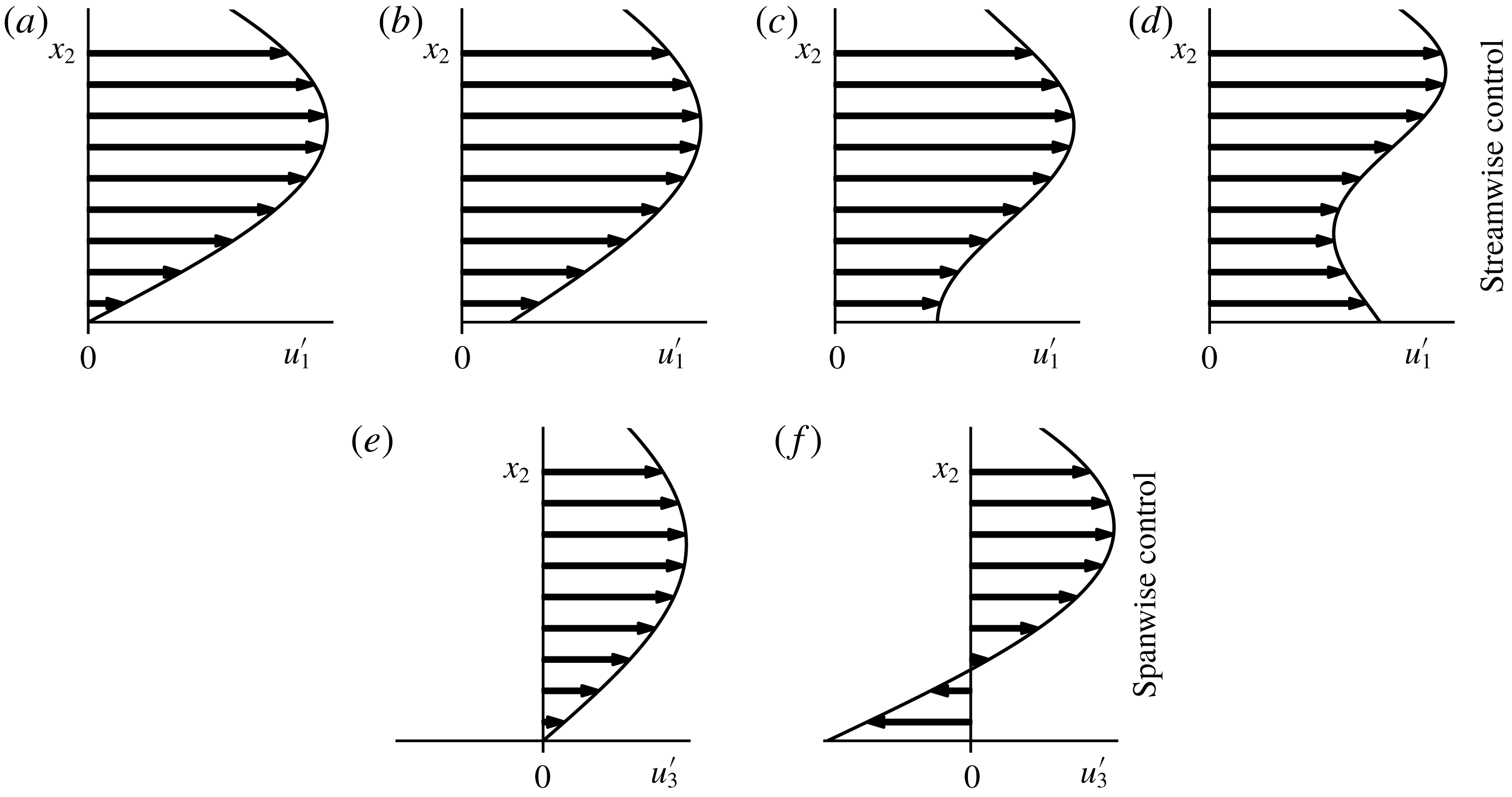
Based on our analysis, active streamwise wall fluctuations lead to drag reduction in three different ways:
(i) Decreased spanwise vorticity fluctuations without reversing their direction at the wall, as shown in figure 11(b). This provides less than 4 % drag reduction.
(ii) Total cancellation of spanwise vorticity fluctuations, as indicated by the tangent of the velocity profile at the wall in figure 11(c). This reduces friction drag by 4 %.
(iii) Decreased or increased spanwise vorticity fluctuations, by reversing their direction at the wall as sketched in figure 11(d). A drag reduction between 4 and 8 % can be achieved.
Active spanwise wall fluctuations are favourable only if the wall velocity increases the streamwise vorticity fluctuations without changing its direction at the wall as shown in figure 11(e,f). This leads to a drag reduction of no more than 25 %.
The question then arises: for how long does a successful control need to apply unidirectional wall motions to sustain the sketched velocity profiles? Figure 11 presents near-wall velocity profiles corresponding to energetic fluid motions. The average duration of unidirectional actuation (
 $t_{act}$
) can be estimated based on the characteristic length scale (
 $L_{c}$
) and convection velocity (
 $U_{c}$
) of such motions as
 $$\begin{eqnarray}t_{act}=\frac{L_{c}}{U_{c}}.\end{eqnarray}$$
The convection velocity of the near-wall flow features is approximately
 $U_{c}=10u_{\unicode[STIX]{x1D70F}}$
(Carpenter et al.
Reference Carpenter, Kudar, Ali, Sen and Davies2007). The characteristic length scale for the streamwise control can be estimated using the streamwise extent of velocity streaks lying between
 $L_{c}=1000\unicode[STIX]{x1D6FF}_{\unicode[STIX]{x1D708}}$
and
 $L_{c}=10\,000\unicode[STIX]{x1D6FF}_{\unicode[STIX]{x1D708}}$
according to Carpenter et al. (Reference Carpenter, Kudar, Ali, Sen and Davies2007) and Jiménez (Reference Jiménez2013). For the spanwise control, the streamwise extent of quasi-streamwise vortices can be estimated as
 $L_{c}=100\unicode[STIX]{x1D6FF}_{\unicode[STIX]{x1D708}}$
given by Jiménez (Reference Jiménez2013). The average duration of unidirectional actuation is therefore between
 $t_{act}=100\unicode[STIX]{x1D6FF}_{\unicode[STIX]{x1D708}}/u_{\unicode[STIX]{x1D70F}}$
and
 $1000\unicode[STIX]{x1D6FF}_{\unicode[STIX]{x1D708}}/u_{\unicode[STIX]{x1D70F}}$
for the streamwise control, and
 $t_{act}=10\unicode[STIX]{x1D6FF}_{\unicode[STIX]{x1D708}}/u_{\unicode[STIX]{x1D70F}}$
for the spanwise control. This indicates that streamwise control requires a wall that can sustain almost unchanged local velocity for a relatively long time. By comparison, the spanwise control requires a higher actuation frequency.
3.2 Passive flow control
If the passively controlled wall cannot sustain one of the velocity profiles depicted in figure 11 for a sufficiently long time, then lower drag reduction is expected compared to active control. Furthermore, increased friction drag is expected (negative drag reduction) if the modified near-wall velocity profiles are the opposite of the beneficial scenarios. Observing figure 11(d,f), we can conclude that the required wall velocities are opposing the wall shear stresses. This means that sustained beneficial spanwise wall velocities would require a power supply. For this reason, spanwise wall velocity control cannot be realised passively and it is expected that passive spanwise wall fluctuations lead to drag increase. For the same reason, the drag reduction peak of the active streamwise control cannot be exploited passively either. However, we hypothesise that the proposed compliant wall model can sustain profiles similar to figure 11(b), and exploit the shear decreasing drag-reduction mechanism of the active streamwise control.
3.2.1 Frequency response based on analytical solutions
Although the drag-reduction potential of compliant walls cannot be predicted analytically, the solutions derived in § 2.2 allow us to validate the shear cancelling ability of in-plane deforming surfaces. Furthermore, the solutions can be utilised to narrow the parameter space of compliant walls and find the region of interest. To this end, analytical tests are conducted for the low Reynolds number case (
 $Re=2857$
,
 $Re_{\unicode[STIX]{x1D70F}}\approx 180$
).
Firstly, the analytical solutions are applied to investigate the frequency response of the surface. The compliant walls represented by damped harmonic oscillator systems are characterised by the undamped natural frequency
 $\unicode[STIX]{x1D714}_{ud}=\sqrt{\unicode[STIX]{x1D6EC}_{s}/\unicode[STIX]{x1D6EC}_{m}}$
and the damping ratio
 $\unicode[STIX]{x1D6FE}=\unicode[STIX]{x1D6EC}_{d}/2/\sqrt{\unicode[STIX]{x1D6EC}_{s}\unicode[STIX]{x1D6EC}_{m}}$
. The wall velocity response as a function of the angular frequency of the oscillating pressure is observed based on figure 12(a). Fluid in the channel acts as additional viscous damping, and so wall oscillations are bounded even when the wall itself is undamped. If the coupled system is underdamped, a resonance peak is present at a frequency somewhat lower than the undamped resonance frequency of the surface. With increasing damping the resonance peak vanishes as the coupled system becomes overdamped. This behaviour is similar to classical damped harmonic oscillators with independent external forcing.
Monoharmonic analyses of the wall velocity and the wall shear stress. Frequency response of the wall velocity (a), and the r.m.s. wall shear stress as a function of the damping parameter (b), inertia parameter (c) and spring parameter (d). For these calculations the pressure gradient amplitude is set to unity (
 $P_{A}=1.0$
).

Considering that drag reduction with the present active controls is linked to the wall-shear-stress fluctuations, attention is turned towards the wall-shear-stress change compared to the baseline case (no-slip wall). Figure 12(b–d) shows that as the surface parameters increase the surface becomes more rigid and the flow converges to the baseline state. Figure 12(b) highlights that total shear cancellation is possible at the resonance frequency only if the wall is undamped (
 $\unicode[STIX]{x1D6EC}_{d}=0$
). Furthermore, shear increase is possible only if the coupled system is underdamped. As the damping parameter increases, compliant walls (i) become less responsive but (ii) interact with the flow in a wider frequency range. On the contrary, figure 12(c,d) shows that increasing inertia and spring parameters cause the responsive frequency range to decrease and the interaction between the fluid and the solid system to weaken.
Secondly, the superposition principle is applied and a semi-analytical model is created to approximate compliant wall behaviour in the turbulent channel flow. The semi-analytical model accounts for multiple Fourier modes that are tuned to be somewhat representative about turbulent wall-shear-stress fluctuations. Modes are computed based on the wall-shear-stress fluctuation history because wall shear stress is the load acting on the proposed compliant wall models. The oscillatory pressure modes of the model are determined so that the wall shear stress in the pulsatile channel flow matches a quasi-periodic turbulent wall-shear-stress signal segment in the baseline turbulent channel flow at a single location. For further details of this procedure we refer to Józsa (Reference Józsa2018). The idealised semi-analytical framework enables rapid prediction of r.m.s. wall shear stress and wall velocity as a function of the control parameters in the turbulent channel flow. Figure 13(a–f) depicts some semi-analytical predictions corresponding to
 $u_{1,p}^{\prime }$
-control with
 $N=15$
and 300 Fourier modes.
Effect of passive control parameters on r.m.s. streamwise wall-shear-stress fluctuations (a–c); r.m.s. wall velocities (d–f); and drag reduction (g–i). DNS results are indicated by circles and squares. The lines correspond to analytical solutions at
 $Re=2857$
, with
 $N=30$
and 300 modes fitted to turbulent signal segments of lengths 1.3 and 11.9 eddy turnover times.

Finally, the region of interest in the parameter space can be identified using the semi-analytical model. According to the monoharmonic analysis the shear cancelling potential increases as the compliant wall parameters approach zero. For this reason, maximal shear increase is sought. Parameters are optimised for the maximum r.m.s. streamwise wall shear stress with
 $N=15$
Fourier modes:
 $$\begin{eqnarray}\text{max}(\unicode[STIX]{x1D70F}_{1,rms}^{\prime });\quad \unicode[STIX]{x1D6EC}_{m}\in [4,\infty ],\unicode[STIX]{x1D6EC}_{d}\in [0,\infty ],\unicode[STIX]{x1D6EC}_{s}\in [0,\infty ].\end{eqnarray}$$
The lower bound of
 $\unicode[STIX]{x1D6EC}_{m}=4$
is given by the numerical stability of the weak coupling scheme at
 $Re_{\unicode[STIX]{x1D70F}}\approx 180$
. Constrained, gradient-based numerical algorithms were tested (Nash Reference Nash1984; Kraft Reference Kraft1988; Byrd et al.
Reference Byrd, Lu, Nocedal and Zhu1995; Zhu et al.
Reference Zhu, Byrd, Lu and Nocedal1997; Nocedal & Wright Reference Nocedal and Wright2006), all of which found the optimum within the restricted parameter space at
 $\unicode[STIX]{x1D6EC}_{m}=4$
,
 $\unicode[STIX]{x1D6EC}_{d}=0$
,
 $\unicode[STIX]{x1D6EC}_{s}=96.59$
. This compliant wall induces intense wall velocities resulting in an r.m.s. wall shear stress
 ${\approx}10\,\%$
higher than the baseline case. This case is identified as
 $u_{1,p}^{\prime }$
Lo0Hi, where the first part refers to the streamwise passive control and the second part contains information about the compliant wall parameters as explained under table 3.
3.2.2 Direct numerical simulation results
The compliant wall
 $u_{1,p}^{\prime }$
Lo0Hi is selected as a starting point to investigate the effect of the three passive control parameters with direct numerical simulations. Parameters relating to the tested compliant walls are listed in the Supplementary materials. Figure 13 summarises the results. A sweep in the spring coefficient is conducted because the frequency analysis indicates that lowering the spring parameter broadens the frequency range of integration and enables more efficient shear cancellation. Figure 13(c,f,i) displays the effect of the spring parameter. The parameter sweep reveals that
 $u_{1,p}^{\prime }$
Lo0Lo (
 $\unicode[STIX]{x1D6EC}_{m}=4$
,
 $\unicode[STIX]{x1D6EC}_{d}=0$
,
 $\unicode[STIX]{x1D6EC}_{s}=1.0$
) is a compliant wall providing 3.68 % drag reduction, the peak value over the parameter space considered herein. This wall achieves drag reduction by decreasing the r.m.s. streamwise wall-shear-stress fluctuations by
 ${\approx}60\,\%$
. The shear increasing–decreasing modes of the compliant walls can be observed in figure 13(c).
Compliant walls promoting streamwise (
 $u_{1,p}^{\prime }$
) and spanwise (
 $u_{3,p}^{\prime }$
) wall fluctuations selected for detailed analysis. The ID is related to the material properties, so that, for instance, ‘
 $u_{1,p}^{\prime }$
Lo0Lo’ is a coating realising passive streamwise control with relatively low inertia parameter, zero damping and low spring parameter. Compliant walls are considered the same if their dimensional inertia, damper and spring parameters are equal. The #column refers to the coating number in the Supplementary materials which includes a complete list of passive control simulations.

Decreasing the spring parameter of an undamped compliant wall with fixed inertia parameter (
 $\unicode[STIX]{x1D6EC}_{m}=4$
) leads to wall-shear-stress cancellation, flattening out at approximately
 $-95\,\%$
as evident in figure 13(c). This substantial shear cancellation requires wall velocities in the order of
 $2u_{\unicode[STIX]{x1D70F}}$
as revealed in figure 13(f). With increasing spring parameter the wall becomes stiffer and the flow converges towards the uncontrolled states. However, before a plateau is reached in figure 13(c) at around
 $\unicode[STIX]{x1D6EC}_{s}=10^{4}$
, a local maximum forms at
 $\unicode[STIX]{x1D6EC}_{s}=10^{2}$
. This peak corresponds to r.m.s. wall-shear-stress increasing behaviour. It is somewhat surprising though that a local maximum is not present in the wall velocity curve in figure 13(f).
The influence of inertia and damping parameters is examined by conducting further direct numerical simulations using
 $u_{1,p}^{\prime }$
Lo0Lo as a starting point. Figure 13(a,b) shows that the wall-shear-stress fluctuations for the given spring parameter
 $\unicode[STIX]{x1D6EC}_{s}=1$
cannot be decreased by more than 60 %. As the inertia and the damping of the compliant wall are raised, the wall behaves increasingly like a no-slip wall and the flow converges towards the uncontrolled state. This means that the compliant wall becomes inactive, as confirmed by
 $\dot{\unicode[STIX]{x1D709}}_{1,rms}^{+}\rightarrow 0$
in figure 13(d,e). The r.m.s. wall-shear-stress and wall velocity trends seem to be qualitatively similar at
 $Re_{\unicode[STIX]{x1D70F}}\approx 180$
and
 ${\approx}1000$
.
Semi-analytical predictions at
 $Re=2857$
provide reasonably good estimates of the described trends. Considering that the input of the semi-analytical model is a wall-shear-stress signal segment from a single location of the baseline turbulent channel flow, it is expected that a sufficiently long signal segment is required for accurate predictions. As the input wall-shear-stress signal segment lengthens, the Fourier transformation includes increasing numbers of low frequency modes which are essential to capture the wall-shear-stress trends accurately. However, these low frequency modes truncate the predictions and introduce non-physical resonance peaks to the r.m.s. wall velocity trends as visible in figure 13(d,f). Even though the
 $\unicode[STIX]{x1D70F}_{1,rms}^{\prime }$
and
 $\dot{\unicode[STIX]{x1D709}}_{1,rms}^{\prime }$
predictions are reasonably acceptable, the results obtained with the semi-analytical model should be treated with caution. Nevertheless, the semi-analytical model approximates satisfactorily the limiting behaviour of the compliant walls. Furthermore, it provides useful insight into the fascinating physics of the fluid–solid system which exhibits different behaviour through six orders of magnitude of the control parameters.
Passive streamwise flow control reduces turbulent friction drag in most of the cases investigated. Maximum drag reduction (3.68 %) is measured for
 $u_{1,p}^{\prime }$
Lo0Lo at
 $Re_{\unicode[STIX]{x1D70F}}\approx 180$
. A similar drag reduction, 3.61 %, is measured for an underdamped compliant wall (
 $u_{1,p}^{\prime }$
LoLoLo in table 3 at
 $Re_{\unicode[STIX]{x1D70F}}\approx 180$
). However, only a 1.47 % drag reduction can be measured with the same compliant wall at
 $Re_{\unicode[STIX]{x1D70F}}\approx 1000$
(
 $u_{1,p}^{\prime }$
LoHiLo in table 3). (Compliant walls are considered the same if their dimensional physical properties are equal.) It seems that even with an idealised compliant surface such as presented in figure 4(b) the achievable drag reduction is rather modest in turbulent boundary layers.
Figure 13(g–i) shows drag-reduction curves as functions of control parameters. As the control parameters tend to zero, shear cancellation becomes more efficient and a peak drag reduction of approximately 4 % occurs at
 $Re_{\unicode[STIX]{x1D70F}}\approx 180$
. Whereas a drag-reduction plateau is reached in figure 13(h,i) at
 $Re_{\unicode[STIX]{x1D70F}}\approx 180$
, the drag reduction in figure 13(g) might increase slightly further if the inertia parameter is decreased. This could not be tested because of the stability limit of the weak coupling scheme.
It is somewhat surprising that at
 $Re_{\unicode[STIX]{x1D70F}}\approx 1000$
the drag reduction curve shows a rapid breakdown with decreasing spring parameter (see figure 13
i). In figure 13(g,h) drag reduction is more or less proportional to r.m.s. wall velocity and inversely proportional to wall-shear-stress change. However, in figure 13(i) maximum drag reduction is measured at
 $\unicode[STIX]{x1D6EC}_{s}=1$
, before the compliant walls exhibit maximum r.m.s. wall velocity and maximum wall-shear-stress cancellation. This finding highlights that
 $\unicode[STIX]{x1D70F}_{1}^{\prime }=0$
(total shear cancellation) is not optimal for passive streamwise control. Correlations between measured drag reduction and modified wall quantities are unclear, and the exact drag-reduction mechanism of the streamwise wall velocity fluctuations remains to be developed.
Whereas the least successful passive streamwise control resulted in a 0.64 % drag increase at
 $Re_{\unicode[STIX]{x1D70F}}\approx 1000$
, the passive spanwise controls give a consistent drag increase ranging from 1.77 to 58.77 % (see, for instance table 3). For the simulation parameters we refer to the Supplementary materials. Considering that (i) spanwise slip leads to increased friction drag (Min & Kim Reference Min and Kim2004), and (ii) in-plane deforming compliant surfaces promote slip condition, it is not surprising that passive spanwise wall motions lead to drag penalty. The results confirm our hypothesis that solely streamwise passive wall fluctuations can modestly decrease friction drag, whereas solely spanwise passive wall fluctuations increase friction drag.
In previous numerical studies on compliant wall drag reduction, it has been demonstrated that simulation parameters, namely averaging time (Xu et al.
Reference Xu, Rempfer and Lumley2003) and computational domain size (Fukagata et al.
Reference Fukagata, Kern, Chatelain, Koumoutsakos and Kasagi2008), have a significant impact on estimating drag reduction. In the present study, a detailed uncertainty quantification is provided for the low Reynolds number channel flow and the most successful passive control (
 $u_{1,p}^{\prime }$
Lo0Lo). To this end, additional simulations were carried out changing the key simulation settings, including (i) spatial resolution; (ii) temporal resolution; (iii) domain size; and (iv) sample size. The total uncertainty (
 $e_{DR}^{total}$
) is estimated as the
 $L_{2}$
-norm of the individual uncertainties multiplied by a safety factor equal to two. This leads to
 $e_{DR}^{total}=\pm 1\,\%$
. Appendix B summarises the results. The uncertainty quantification justifies the drag-reduction capabilities of in-plane passive wall fluctuations.
In the present study, the parameters of compliant walls have been mapped throughout six orders of magnitude. The question arises as to whether the simulated parameters can be used for designing a functional prototype. A compliant wall prototype has been devised based on the rotating disc model in figure 4(b). Detailed comments on the realisation are given in appendix C where parameters are chosen to preserve a hydrodynamically smooth surface. The constraints lead to a geometrical arrangement with only half of the surface being covered with moving elements; hence the expected drag reduction is
 ${\approx}1\,\%$
.
In order to evaluate the second part of the hypothesis, namely that,
 $u_{1,p}^{\prime }$
-control can sustain the same drag-reduction mechanism as
 $u_{1,a}^{\prime }$
-control, certain turbulence statistics are investigated. Figure 7 displays the Reynolds stresses in the channels obtained for the most successful active and passive controls. The active streamwise controls,
 $u_{1,p}^{\prime }$
Lo0Lo at
 $Re_{\unicode[STIX]{x1D70F}}\approx 180$
, and
 $u_{1,p}^{\prime }$
LoLoLo at
 $Re_{\unicode[STIX]{x1D70F}}\approx 1000$
result in qualitatively similar Reynolds stress trends. However, even the most flexible compliant wall cannot support wall fluctuations with as high amplitude as the active control according to figure 7(a,b). This is because of the flattening of the near-wall fluctuating velocity profile which inevitably leads to decreased wall-shear-stress fluctuations, and hence the lack of driving force which could accelerate the compliant wall further.
Premultiplied energy spectra of the streamwise fluctuations as a function of wall distance and spanwise wavelength (
 $\unicode[STIX]{x1D706}_{3}$
). Here
 $k_{3}$
is the spanwise angular wavenumber and
 $E_{11}$
denotes the streamwise energy spectra.

Figure 14 displays the premultiplied streamwise energy spectra in terms of wall distance and spanwise wavelength. The peaks centred about
 $x_{2}^{+}=15$
and characteristic wavelength approximately 100 viscous units correspond to near-wall velocity streaks (Kline et al.
Reference Kline, Reynolds, Schraub and Runstadler1967; Jiménez & Pinelli Reference Jiménez and Pinelli1999) both at
 $Re_{\unicode[STIX]{x1D70F}}\approx 180$
in figure 14(a) and
 $Re_{\unicode[STIX]{x1D70F}}\approx 1000$
in figure 14(b). Energetic large-scale motions in the log layer (Balakumar & Adrian Reference Balakumar and Adrian2007; Hutchins & Marusic Reference Hutchins and Marusic2007) can be observed at
 $Re_{\unicode[STIX]{x1D70F}}\approx 1000$
in figure 14(b) above
 $x_{2}^{+}=100$
, with wavelengths ranging between
 ${\approx}300$
and 3000. Figure 14(c,d) indicates that the
 $u_{1,a}^{\prime }$
-control energises remarkably the near-wall streamwise fluctuations. Figure 14(c–f) shows that both
 $u_{1,a}^{\prime }$
and
 $u_{1,p}^{\prime }$
-controls have greatest impact over a relatively narrow wavelength range between 100 and 200 viscous units associated with streamwise velocity streaks. When successful, the passive streamwise control energises the streamwise fluctuations in the viscous sublayer in a similar fashion to the active
 $u_{1,a}^{\prime }$
-control with
 $x_{2,c}^{+}=1$
. Even though compliant walls cannot provide such strong amplification of near-wall events.
The performance degradation of the controls at
 $Re_{\unicode[STIX]{x1D70F}}\approx 1000$
is probably due to the formation of large-scale motions in the log layer. These large-scale events make an increasing contribution to the Reynolds shear stresses, and hence to skin friction at increasing Reynolds numbers (Hutchins & Marusic Reference Hutchins and Marusic2007; Touber & Leschziner Reference Touber and Leschziner2012). Modification of these outer layer structures is a major challenge for future control development. Mathis, Hutchins & Marusic (Reference Mathis, Hutchins and Marusic2009) and Ganapathisubramani et al. (Reference Ganapathisubramani, Hutchins, Monty, Chung and Marusic2012) demonstrated that the large-scale motions influence the near-wall velocity streaks through frequency and amplitude modulation. Figure 14(d,f) suggests that the introduced streamwise wall motions are capable of a weak reversed modulation. The modified spectra shed light on a strengthened connection between near-wall events and the large-scale motions of the log layer as visualised by the consistent contours stretching from
 $x_{2}^{+}=1$
to 700. It is somewhat counter-intuitive that the energised streaks and strengthened connection between near-wall and log-layer events lead to a slight drop in the streamwise Reynolds stress fluctuations (see figure 7(b) above
 $x_{2}^{+}=100$
). The evidence from Reynolds stress and vorticity statistics in figures 7 and 8, and turbulence spectra in figure 14 confirms that the
 $u_{1,p}^{\prime }$
-control modifies the flow similarly to
 $u_{1,a}^{\prime }$
-control with
 $x_{2,c}^{+}=1$
.
Given that the compliant walls considered herein do not restrict wall displacements, and exhibit intensive velocities, we quantify the wall displacement responsible for observed drag increase and drag reduction. The introduced wall motions are unidirectional and depend on two spatial coordinates. This means that an incompressible, isotropic surface cannot sustain the modelled wall velocities. To assess whether such wall motions could occur using a compressible material, and identify the challenges related to the physical realisation, the Lagrangian displacement field on the wall is examined. The velocity of Lagrangian particles on the wall is equivalent to the computed wall velocity (
 $\dot{\unicode[STIX]{x1D709}}_{i}$
) at every point. Displacements of the material points are integrated using a first-order forward Euler scheme. Table 4 presents the results obtained with passive flow controls after 1.25 eddy turnover times, along with displacements corresponding to active controls.
Results of Lagrangian wall displacement analysis at
 $Re_{\unicode[STIX]{x1D70F}}\approx 180$
after 1.25 eddy turnover times.

Noting that the coating deformations are driven by streamwise velocity streaks in the case of wall-shear-stress decreasing passive streamwise control, the displacements can be estimated from the average properties of the streaks. A material point is influenced by a high/low momentum region (streak) as long as the region is convected downstream above the point. The time taken can be estimated from the streak length, convection velocity and r.m.s. wall velocity (computed by analytical solutions or DNS). Then a Lagrangian particle needs to move in the same direction for a time equal to
 $$\begin{eqnarray}t_{unidir.~motion}=\frac{L_{c}}{U_{c}-\dot{\unicode[STIX]{x1D709}}_{1,rms}}.\end{eqnarray}$$
The average streamwise Lagrangian displacement (
 $\unicode[STIX]{x1D709}_{1,rms}^{{\mathcal{L}}}$
) can then be approximated by
 $$\begin{eqnarray}\unicode[STIX]{x1D709}_{1,estimated}^{{\mathcal{L}}}=\dot{\unicode[STIX]{x1D709}}_{1,rms}t_{unidir.~motion}.\end{eqnarray}$$
Assuming that the streaks are unchanged by the control, the estimated typical Lagrangian displacement ranges from 100 to 1000 viscous units for
 $u_{1,p}^{\prime }$
LoHiLo and from 200 to 2000 viscous units for
 $u_{1,p}^{\prime }$
LoLoLo. A unidirectional motion lasting for 1.25 eddy turnover times leads to displacements of 230 and 460 viscous units for
 $u_{1,p}^{\prime }$
LoHiLo and
 $u_{1,p}^{\prime }$
LoLoLo respectively. This is in satisfactory agreement with the values presented in table 4. The computed deformations are expected to show an inner scaling with Reynolds number because they are strongly related to sublayer streaks (scaling with
 $\unicode[STIX]{x1D6FF}_{\unicode[STIX]{x1D708}}$
and
 $u_{\unicode[STIX]{x1D70F}}$
). Similar calculations might be conducted based on the characteristic properties of quasi-streamwise vortices to estimate the displacements required for active and passive spanwise controls. However, such calculations cannot be carried out when wall motions are determined by impulsive load changes present between high and low momentum regions (for instance,
 $u_{1,p}^{\prime }$
Lo0Hi).
Active and passive streamwise controls require relatively large displacements of the wall. The wall needs to support large deformations in the positive and negative directions within a short distance (approximately 100
 $\unicode[STIX]{x1D6FF}_{\unicode[STIX]{x1D708}}$
) in order to cancel wall shear stress fluctuations originating from streaks. Such behaviour is difficult to imagine beyond the rotating disc model in figure 4(b). Compared to streamwise controls the spanwise controls exhibit one order of magnitude smaller wall displacements. Spanwise wall displacements of the order of
 $\unicode[STIX]{x1D6FF}_{\unicode[STIX]{x1D708}}$
increase friction drag considerably. As long as compliant walls cannot utilise the drag reducing potential of spanwise wall motions, the spanwise rigidity of compliant walls should be as high as possible to avoid a drag penalty. This finding underlines the necessity of investigating anisotropic walls, as also proposed by Yeo (Reference Yeo1990), Carpenter & Morris (Reference Carpenter and Morris1990), Fukagata et al. (Reference Fukagata, Kern, Chatelain, Koumoutsakos and Kasagi2008) and Luhar et al. (Reference Luhar, Sharma and McKeon2015).
4 Conclusions
This study has investigated the effect of solely in-plane active and passive wall fluctuations on fully turbulent canonical channel flows at low and intermediate friction Reynolds numbers. Direct numerical simulations were in close agreement with spectral DNS results obtained by Lee & Moser (Reference Lee and Moser2015) for fully turbulent flow in a rectangular channel with stationary walls. Active and passive flow controls were modelled using periodic in-plane wall velocity conditions following Choi et al. (Reference Choi, Moin and Kim1994). It was found that active streamwise control could provide drag reductions of 8 % at low (
 $Re_{\unicode[STIX]{x1D70F}}\approx 180$
) and 7 % at intermediate (
 $Re_{\unicode[STIX]{x1D70F}}\approx 1000$
) friction Reynolds numbers. Active spanwise control led to drag reduction more than 19 %, primarily because the wall motions counteracted quasi-streamwise vortices and steepened the near-wall velocity profile (wall-shear-stress increasing mode). Conversely, streamwise control utilises wall motions in the same direction as the near-wall streamwise velocity fluctuations, and also provides drag reduction in wall shear stress increasing and decreasing modes.
Analytical solutions of pulsatile channel flow and direct numerical simulations indicated that positive streamwise wall fluctuations can lead to 3.7 % and 2.3 % drag reductions at low and intermediate friction Reynolds numbers, depending on the control parameters. Our results show that the superior performance of active spanwise control cannot be exploited passively, and passive spanwise wall fluctuations can result in a drag penalty exceeding 50 %. Analysis of the Lagrangian displacement of the wall showed that streamwise displacements of the order of 1000 viscous length scales are required to obtain drag reduction solely by means of streamwise wall fluctuations. However, solely spanwise wall displacements of the order of 1 viscous length scale can lead to a drag increase of approximately 4 %. For the first time, it has been shown that passive wall fluctuations can decrease friction drag in fully turbulent wall-bounded flows by exploiting the same drag-reduction mechanism as a well-established active control. These results highlight the importance of material anisotropy in compliant wall design and may eventually have repercussions for drag-reduction measures in practice.
Acknowledgement
The authors are grateful to AkzoNobel’s Marine Coatings business (International Paint Ltd) and the Energy Technology Partnership [ETP106] for financial support. DNS computations were carried out on the ARCHER UK National Supercomputing Service (http://www.archer.ac.uk).
Supplementary data
Supplementary data is available at https://doi.org/10.1017/jfm.2019.145.
Appendix A
The equation of motion of an individual disc in figure 4(b) is
 $$\begin{eqnarray}C_{m}^{\ast }\ddot{\unicode[STIX]{x1D703}}_{i}^{\ast }+C_{d}^{\ast }\dot{\unicode[STIX]{x1D703}}_{i}^{\ast }+C_{s}^{\ast }\unicode[STIX]{x1D703}_{i}^{\ast }=T_{f}^{\ast },\end{eqnarray}$$
where
 $\unicode[STIX]{x1D703}_{i}^{\ast }$
denotes angular displacement,
 $\dot{\unicode[STIX]{x1D703}}_{i}^{\ast }$
angular velocity,
 $\ddot{\unicode[STIX]{x1D703}}_{i}^{\ast }$
angular acceleration and
 $T_{f}^{\ast }$
torque acting on the disc. The
 $i$
subscript is used to differentiate between discs with spanwise aligned axis (
 $i=1$
) and streamwise aligned axis (
 $i=3$
). The coefficients
 $C_{m}^{\ast }$
,
 $C_{d}^{\ast }$
and
 $C_{s}^{\ast }$
are the moment of inertia, the viscous damping coefficient and the torsion spring coefficient, respectively. For simplicity, the damping coefficient is assumed constant.
Throughout this study, the mounted discs are designed so that they preserve a hydrodynamically smooth surface; hence,
 $D^{\ast }(1-\cos \unicode[STIX]{x1D6FD})/2\leqslant 5\unicode[STIX]{x1D6FF}_{\unicode[STIX]{x1D708}}^{\ast }$
based on figure 4(b). The wall velocity induced by a disc is approximated by the tangential velocity of the disc (
 $D^{\ast }\dot{\unicode[STIX]{x1D703}}_{i}^{\ast }/2=\dot{\unicode[STIX]{x1D709}}_{i}^{\ast }\approx u_{i,wall}^{\ast }$
). This assumption leads to less than 5 % error in the induced wall velocity so long as
 $\unicode[STIX]{x1D6FD}\leqslant \unicode[STIX]{x03C0}/6$
. With these geometrical restrictions in mind, the torque can be estimated from the wall shear stress as
 $T_{f}^{\ast }\approx D^{\ast }A_{s}^{\ast }\unicode[STIX]{x1D70F}_{i}^{\ast }/2$
where
 $A_{s}^{\ast }\approx D^{\ast }H_{D}^{\ast }\unicode[STIX]{x1D6FD}$
is the disc surface area in contact with the fluid, calculated from the disc height
 $H_{D}^{\ast }$
. Substituting the simplified torque formula into (A 1), replacing the angular displacement (
 $\unicode[STIX]{x1D703}_{i}^{\ast }$
) with tangential displacement (
 $\unicode[STIX]{x1D709}_{i}^{\ast }$
), and rearranging lead to
 $$\begin{eqnarray}\frac{2C_{m}^{\ast }}{D^{\ast }}\ddot{\unicode[STIX]{x1D709}}_{i}^{\ast }+\frac{2C_{d}^{\ast }}{D^{\ast }}\dot{\unicode[STIX]{x1D709}}_{i}^{\ast }+\frac{2C_{s}^{\ast }}{D^{\ast }}\unicode[STIX]{x1D709}_{i}^{\ast }=\frac{D^{\ast }}{2}A_{s}^{\ast }\underbrace{\unicode[STIX]{x1D70C}^{\ast }\unicode[STIX]{x1D708}^{\ast }\frac{\unicode[STIX]{x2202}u_{i}^{\ast }}{\unicode[STIX]{x2202}x_{2}^{\ast }}\bigg|_{wall}}_{\unicode[STIX]{x1D70F}_{i}^{\ast }}.\end{eqnarray}$$
The coefficients in (A 2) can be rewritten as
 $\unicode[STIX]{x1D6EC}_{j}^{\ast }=4C_{j}^{\ast }/D^{\ast 2}/A_{s}^{\ast }/\unicode[STIX]{x1D70C}^{\ast }\unicode[STIX]{x1D708}^{\ast }$
, with
 $j=m$
denoting the inertia parameter,
 $j=d$
the damper parameter and
 $j=s$
the spring parameter incorporating the physical properties of the mounted discs as well as the fluid flow. In dimensionless form using
 $\unicode[STIX]{x1D6FF}^{\ast }$
,
 $u_{b}^{\ast }$
,
 $\unicode[STIX]{x1D70C}^{\ast }$
, and
 $\unicode[STIX]{x1D708}^{\ast }$
, equation (A 2) becomes
 $$\begin{eqnarray}\underbrace{\frac{4C_{m}Re}{D^{2}A_{s}}}_{\unicode[STIX]{x1D6EC}_{m}}\ddot{\unicode[STIX]{x1D709}_{i}}+\underbrace{\frac{4C_{d}Re}{D^{2}A_{s}}}_{\unicode[STIX]{x1D6EC}_{d}}\dot{\unicode[STIX]{x1D709}_{i}}+\underbrace{\frac{4C_{s}Re}{D^{2}A_{s}}}_{\unicode[STIX]{x1D6EC}_{s}}\unicode[STIX]{x1D709}_{i}=\frac{\unicode[STIX]{x2202}u_{i}}{\unicode[STIX]{x2202}x_{2}}.\end{eqnarray}$$
Equation (A 3) is equivalent to (2.5) and highlights the influence of the dimensionless control parameters.
Appendix B
The uncertainty originating from various error sources is quantified following the procedure described below:
(i) Truncation error from spatial resolution: baseline and controlled channel flow simulations are repeated on medium and coarse grids. Retaining the case with default settings as the fine grid, the number of cells is halved, and halved again, as presented in figure 15(a). The related drag-reduction uncertainty is estimated as the difference between the grid-independent value obtained by Richardson extrapolation (Roache Reference Roache1998) and the value measured on the fine grid:
$e_{DR}^{spat}=\pm 0.02\,\%$
.(ii) Truncation error from temporal resolution: baseline and controlled channel flow simulations are repeated with a doubled and a halved time step size as shown in figure 15(b). The related drag-reduction uncertainty is estimated as the difference between the ‘fine’ and ‘medium’ time step values:
$e_{DR}^{temp}=\pm 0.08\,\%$
.(iii) Modelling error from domain size: baseline and controlled channel flow simulations are repeated in a domain doubled and halved both in the streamwise and the spanwise directions as displayed in figure 15(c). The related drag-reduction uncertainty is estimated as the difference between the ‘large’ and ‘medium’ domain values:
$e_{DR}^{dom}=\pm 0.48\,\%$
.(iv) Sampling error from finite sample size: figure 15(d) shows the drag reduction if only every second, third, etc. pressure gradient value is taken from the series. The drag-reduction value remains unchanged even if only every one in a hundred elements of the series are kept (value corresponding to
$5\times 10^{-4}$
in figure 15
d). Sampling error is computed for baseline and controlled channel flows using the method described by Trenberth (Reference Trenberth1984) and Oliver et al. (Reference Oliver, Malaya, Ulerich and Moser2014). The related drag-reduction uncertainty is then estimated based on the uncertainty propagation using (3.1):
$e_{DR}^{smpl}=\pm 0.01\,\%$
.


Effect of simulation settings on drag reduction measured with
 $u_{1,p}^{\prime }$
Lo0Lo: spatial resolution (a); temporal resolution (b); domain size (c); and sample size (d). The arrows indicate the default simulation results.

Appendix C
This appendix presents some basic calculations related to the realisation of a wall-shear-stress-driven surface promoting streamwise wall fluctuations. A water channel with
 $L_{2}^{\ast }=0.2$
m height is considered, with intermediate Reynolds number,
 $Re_{\unicode[STIX]{x1D70F}}=1000$
. Such flow conditions can be tested in various experimental facilities (Schultz & Flack Reference Schultz and Flack2013; Zhang et al.
Reference Zhang, Wang, Blake and Katz2017). The #40 parameter set (equivalent to #44) is used because this compliant wall model leads to drag reduction in both low and intermediate Reynolds number channel flows.
The diameter of the discs is set to 5 mm and
 $\unicode[STIX]{x1D6FD}=\unicode[STIX]{x03C0}/6$
rad. The axis of the discs is located at an elevation 2.2 mm below the channel wall. The penetration of the discs into the channel is
 $3.3\unicode[STIX]{x1D6FF}_{\unicode[STIX]{x1D708}}^{\ast }$
so that a hydrodynamically smooth wall is preserved. The height of each discs is chosen based on the spanwise wavelength of the streaks because the discs need to support opposing wall velocities within this distance. The disc height 3 mm is determined so that there are about 5 discs below each high/low momentum region (streaks). Based on the inertia parameter defined in appendix A, the corresponding disc density is
 $40~\text{kg}~\text{m}^{-3}$
, typical of polymer foams, such as expanded polystyrene (EPS) (Horvath Reference Horvath1994) and polyurethane (PU) (Thirumal et al.
Reference Thirumal, Khastgir, Singha, Manjunath and Naik2008). With these design parameters only half of the surface can be covered with moving elements.
If a constant moment of inertia is considered, decreasing the disc diameter proportionally increases the density. Hollow and composite structures can be considered to broaden the palette of suitable materials and overcome difficulties originating from low density requirements. The simulation parameters provide a relatively large degree of freedom, suggesting that a feasible design should be a compromise between size and density. If the minimum disc diameter is approximately 1 mm, then the disc density needs to be a fraction of the fluid density. This suggests that passive control of turbulent flows in low-density fluids (for instance air) can face serious stumbling blocks.
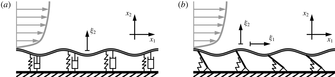


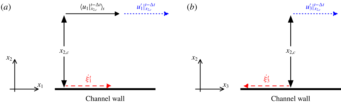


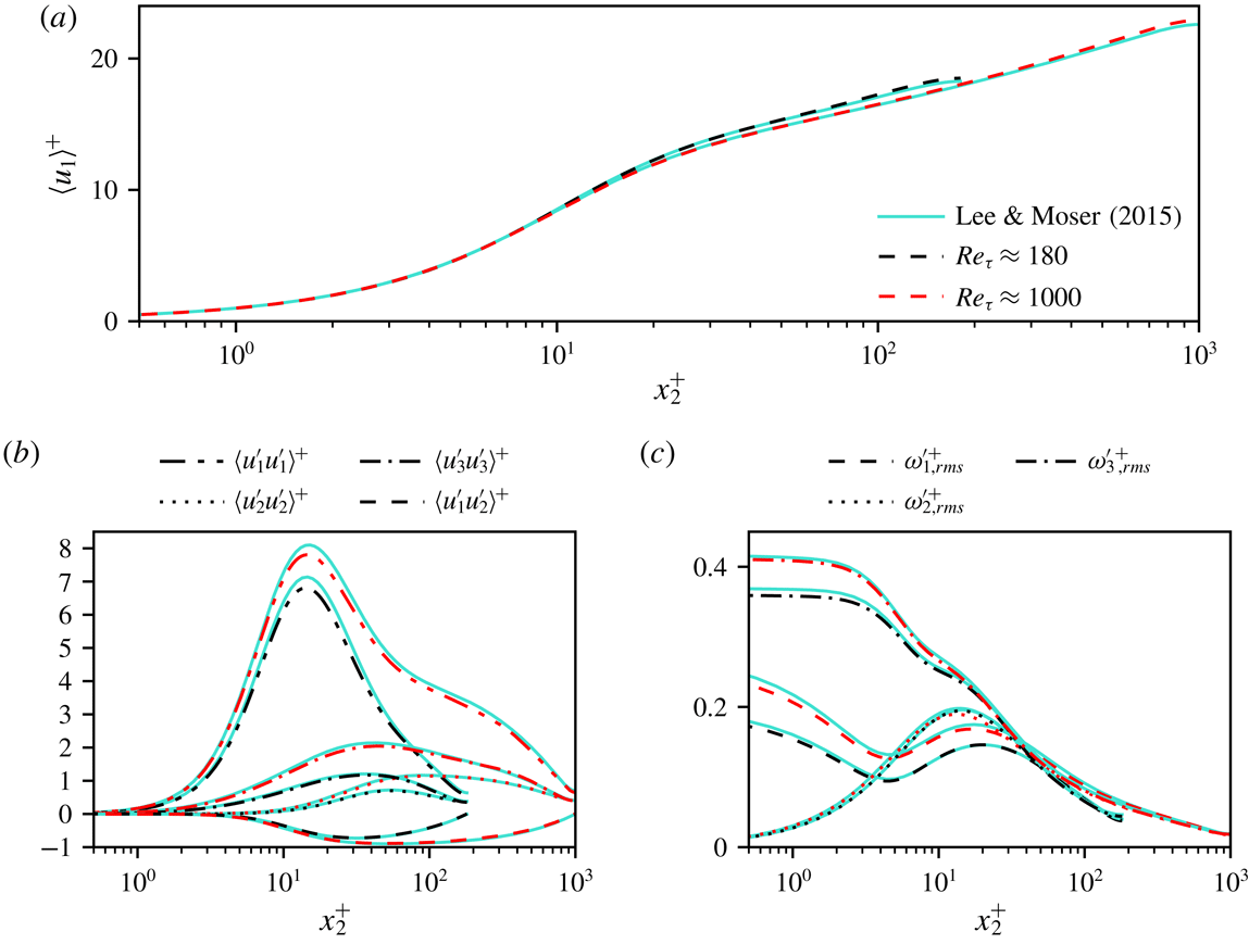

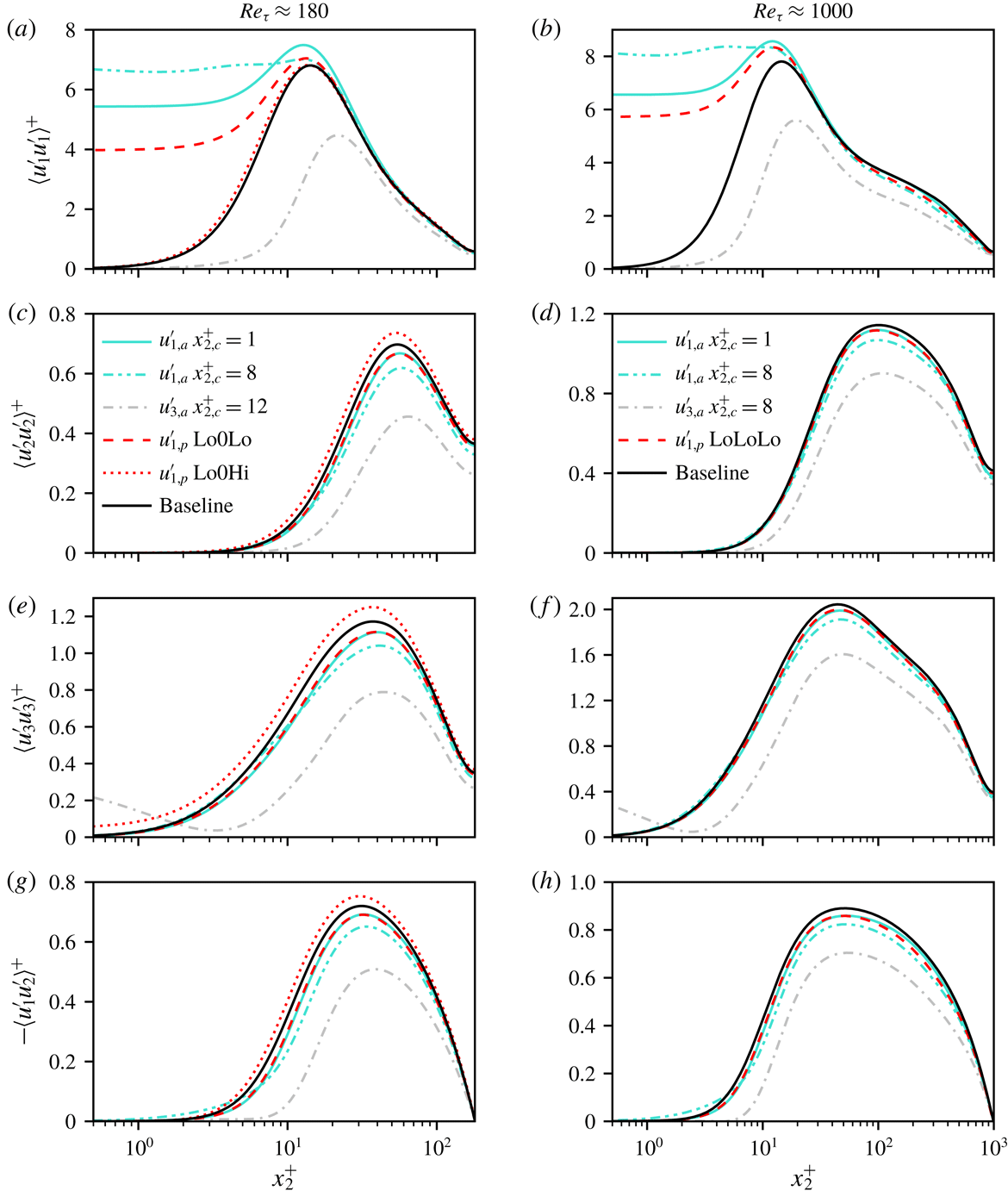

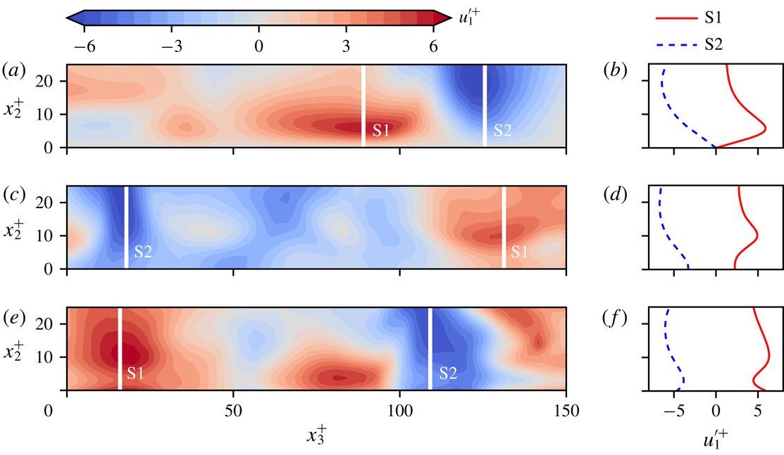
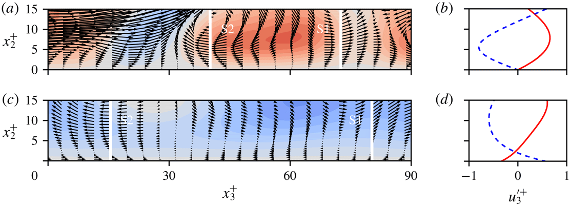

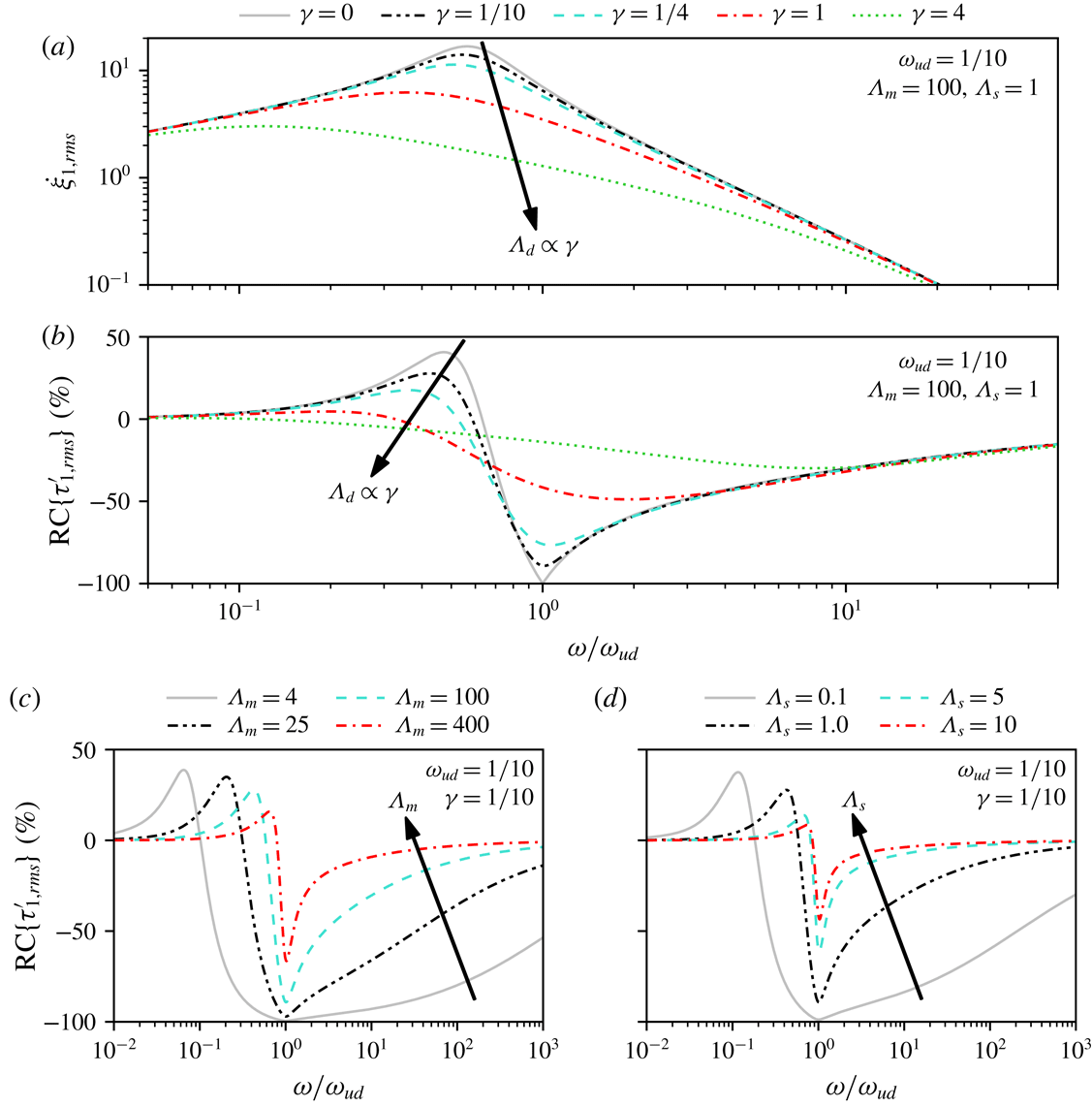


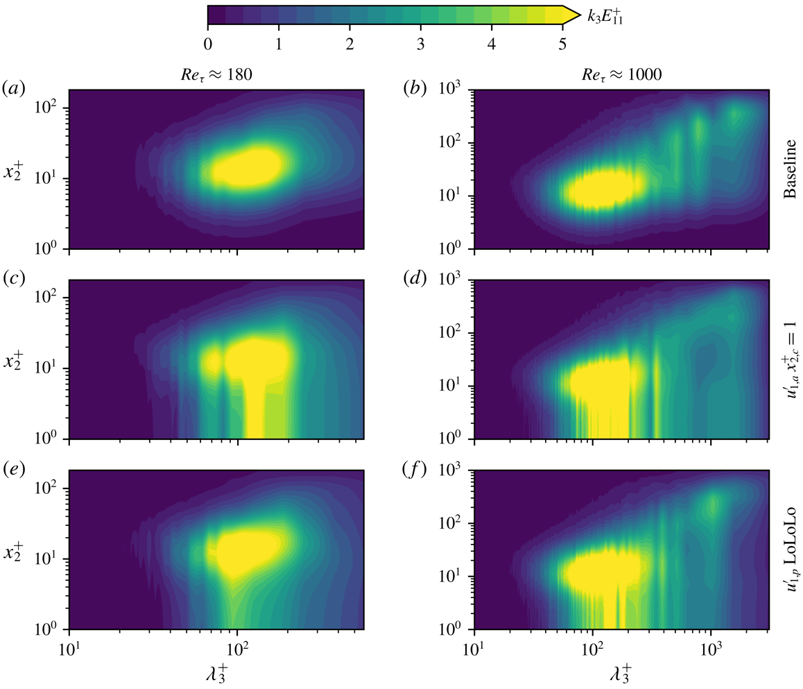


 Open access

