1 Introduction
1.1 Literature review
In the study of hydrodynamic stability, one aims to find out if a given flow state is stable or unstable, and if so, how these instabilities lead to turbulence. Conventional hydrodynamic stability methods involve linearization of the Navier–Stokes equations around a base flow followed by spectral analysis, which aims to identify the Reynolds number
 $Re$
at which the solution becomes unstable (Drazin & Reid Reference Drazin and Reid1981). However, the gap between the linear stability limits and the ones observed in experiments is often significant, with flows routinely transitioning to turbulence well below the critical Reynolds number identified in the analysis (a phenomenon referred to as sub-critical transition). This discrepancy has long been attributed to the use of the linearized Navier–Stokes operator (Trefethen et al.
Reference Trefethen, Trefethen, Reddy and Driscoll1993). Other theoretical methods for studying the stability of flows are often based on spectral truncation of the Navier–Stokes equations into a system of ordinary differential equations (ODEs). However, this approach can lead to truncation errors thereby creating a mismatch between the dynamics of the truncated model and the partial differential Navier–Stokes equations. Both of these drawbacks were addressed in Goulart & Chernyshenko (Reference Goulart and Chernyshenko2012) and Chernyshenko et al. (Reference Chernyshenko, Goulart, Huang and Papachristodoulou2014), where the authors introduced a method involving keeping a number of modes from the Galerkin expansion of the nonlinear Navier–Stokes equations and bounding the energy of the remaining modes, leading to a nonlinear ODE description of the flow dynamics. The resulting ODE description allowed for techniques from control theory, such as Lyapunov’s direct method (Khalil Reference Khalil1996), to be used to study stability and was implemented computationally based on sum-of-squares programming (Parrilo Reference Parrilo2000). It was shown in Huang et al. (Reference Huang, Chernyshenko, Goulart, Lasagna, Tutty and Fuentes2015) that, in the case of rotating Couette flow, this method can find a global stability limit, which is better than the energy method but not as good as the linear stability limit (recall that the linear stability and the global stability limits coincide for Taylor–Couette flow (Taylor Reference Taylor1923)).
Even in the seminal paper by Reynolds (Reference Reynolds1883), it was observed that external excitations and body forces play an important role in flow instabilities. Mechanisms such as energy amplification of external excitations and body forcings have been shown to be crucial in understanding transition to turbulence, as highlighted by Joseph (Reference Joseph1976). Therefore, instead of studying stability, researchers began to focus on energy growth and were able to uncover additional flow properties through the new paradigm of input–output analysis. This led to a focus on so-called transient growth as a primary factor for sub-critical transition to turbulence; i.e. although the perturbations to the linearized Navier–Stokes equation are stable (the eigenvalues have negative real parts), they undergo high-amplitude transient amplifications that steer the trajectories out of the region of linearization. The root cause of the transient growth phenomenon is the non-normality of the stable Navier–Stokes operator that has been linearized about a base flow. The focus on energy growth and the associated input–output properties of the flow has led to the study of the resolvent operator or
 $\unicode[STIX]{x1D700}$
-pseudospectra to uncover when transition occurs, based on the general solution to the linearized Navier–Stokes equations (Schmid Reference Schmid2007). In particular, McKeon & Sharma (Reference McKeon and Sharma2010) used resolvent analysis to study the amplification scalings from an input composed of nonlinear terms and periodic forcings for turbulent pipe flows.
The input–output properties can be characterized based on the class of forcings (stochastic noise versus square integrable signals) and the flow model (linear versus nonlinear and finite-dimensional versus infinite-dimensional) that one considers. For stochastic forcings (Gaussian noise), energy amplification to the linearized Navier–Stokes equations in wall-bounded shear flows was studied by Farrell & Ioannou (Reference Farrell and Ioannou1993). In a similar vein, Bamieh & Dahleh (Reference Bamieh and Dahleh2001) used the stochastically forced linearized Navier–Stokes equation to show that the input–output energy amplification from streamwise-constant excitations to perturbation velocities in channel flows is proportional to
 $Re^{3}$
. The amplification scaling of the linearized Navier–Stokes equation was further characterized in Jovanović (Reference Jovanović2004) and Jovanović & Bamieh (Reference Jovanović and Bamieh2005), where the authors studied the influence of each component of the body forces. For square integrable forcings, Jovanović (Reference Jovanović2004, chap. 9) and Jovanović & Bamieh (Reference Jovanović and Bamieh2005) provided worst-case amplification scalings for incompressible viscous channel flows based on the linearized Navier–Stokes equations. However, an input–output analysis for the nonlinear (partial differential equation, PDE) flow model is absent from the literature.
1.2 Contribution
Our work extends the input–output analysis paradigm. Specifically, we propose a method based on dissipation inequalities (Willems Reference Willems1972) to study input–output amplification in wall-bounded shear flows. This method extends previous results in the following ways. First, it applies directly to nonlinear PDE models of the flow rather than linearized (Vazquez & Krstic Reference Vazquez and Krstic2008) or nonlinear equations that have been discretized and projected onto finite bases. We extend the class of forcings studied in previous work from square integrable forcings to persistent but bounded disturbances, which allows us to analyse both traditional notions of input–output flow properties (e.g. energy amplification and disturbance amplification) as well as new stability properties such as the control theoretic notion of input-to-state stability (ISS). The latter refers to the stability of the flow field under persistent deterministic excitations, which has not been previously analysed. Our technique has the added advantage of enabling the study of multiple input–output flow properties for a broad class of wall-bounded shear flows within a single framework.
One important observation from previous work on input–output analysis is the importance of streamwise-constant perturbations; see e.g. Gustavsson (Reference Gustavsson1991a ), Farrell & Ioannou (Reference Farrell and Ioannou1993) and Jovanović & Bamieh (Reference Jovanović and Bamieh2005). The importance of streamwise-constant structures is also supported with experimental observations of the ubiquity of streamwise-coherent structures; see e.g. Kline et al. (Reference Kline, Reynolds, Schraub and Runstadler1967), Bullock, Cooper & Abernathy (Reference Bullock, Cooper and Abernathy1978), Kim & Adrian (Reference Kim and Adrian1999) and Hutchins & Marusic (Reference Hutchins and Marusic2007) and analysis showing that streamwise-constant models reproduce important flow properties (Gayme et al. Reference Gayme, McKeon, Papachristodoulou, Bamieh and Doyle2010, Reference Gayme, McKeon, Bamieh, Papachristodoulou and Doyle2011). We therefore focus on this class of problems.
We complement the analysis framework by providing a computationally tractable method for the evaluation of input–output properties by solving a convex optimization (Boyd & Vandenberghe Reference Boyd and Vandenberghe2004) problem. Convex optimization problems can be solved efficiently by interior-point methods (Nesterov & Nemirovskii Reference Nesterov and Nemirovskii1994) and there are several tools available for solving them (see e.g. Grant, Boyd & Ye Reference Grant, Boyd and Ye2008). The strength of the method is that the results can be directly extended to more complex flow geometries as long as they can be described or approximated (Weihs Reference Weihs1975; Rubin & Khosla Reference Rubin and Khosla1977) by semi-algebraic sets, i.e. sets characterized by a number of polynomial equalities and inequalities.
We apply then the theory and computational tools to compute the input–output properties of streamwise-constant plane Couette, plane Poiseuille and Hagen–Poiseuille flows. Our results lead to upper bounds that are consistent with the transient growth results in the literature. For channel flows, we show that the upper bounds obtained using our method agree with the results in Jovanović & Bamieh (Reference Jovanović and Bamieh2005) and Jovanović (Reference Jovanović2004, chap. 9) in terms of worst-case disturbance amplification and we show that our framework can be used to study pipe flows as well. Moreover, we observe that the stability bounds to persistent forcings and the experimental Reynolds numbers for transition to turbulence are very similar.
Preliminary mathematical results related to this work were presented in Ahmadi, Valmorbida & Papachristodoulou (Reference Ahmadi, Valmorbida and Papachristodoulou2015). The current paper is different from Ahmadi et al. (Reference Ahmadi, Valmorbida and Papachristodoulou2015) in several aspects. From a theoretical standpoint, the current paper provides a method for energy growth analysis and extends the formulation to both flows between parallel plates and flows in pipes. In addition, it presents the mathematical proofs of the input–output analysis framework and the computational formulation based on convex optimization. From the examples standpoint, we applied the framework to investigate the input–output properties of plane Couette flow, plane Poiseuille and Hagen–Poiseuille flow. Furthermore, the current paper includes a detailed comparison with previous results in the literature and an examination of flow structures corresponding to maximum input–output amplifications.
1.3 Organization
In the next section, we briefly describe the flow model studied in the paper. In § 3, we propose the flow input–output analysis framework based on dissipation inequalities. In § 4, we show how the input–output analysis can be computationally implemented as the solution to a convex optimization problem. In § 5, we demonstrate the effectiveness of the proposed framework by applying it to study input–output properties of plane Couette flow, plane Poiseuille flow and Hagen–Poiseuille flow. Finally, in § 6, we present some concluding remarks and provide directions for future research.
2 The flow perturbation model
We consider the dynamics of forced incompressible shear flows in a given domain with time-independent boundary conditions. The instantaneous flow velocity
 $\bar{\boldsymbol{u}}(t,x)$
,
 $\bar{\boldsymbol{u}}:\mathbb{R}_{{\geqslant}0}\times \unicode[STIX]{x1D6FA}\rightarrow \mathbb{R}^{3}$
, and pressure
 $\bar{p}(t,x)$
,
 $\bar{p}:\mathbb{R}_{{\geqslant}0}\times \unicode[STIX]{x1D6FA}\rightarrow \mathbb{R}$
, are governed by the Navier–Stokes equations
 $$\begin{eqnarray}\left.\begin{array}{@{}c@{}}\displaystyle \unicode[STIX]{x2202}_{t}\bar{\boldsymbol{u}}=\frac{1}{Re}\unicode[STIX]{x1D6FB}^{2}\bar{\boldsymbol{u}}-\bar{\boldsymbol{u}}\boldsymbol{\cdot }\unicode[STIX]{x1D735}\bar{\boldsymbol{u}}-\unicode[STIX]{x1D735}\bar{p}+\boldsymbol{d},\\ \displaystyle 0=\unicode[STIX]{x1D735}\boldsymbol{\cdot }\bar{\boldsymbol{u}},\end{array}\right\}\end{eqnarray}$$
where
 $t>0$
,
 $x\in \unicode[STIX]{x1D6FA}=\unicode[STIX]{x1D6FA}_{i}\times \unicode[STIX]{x1D6FA}_{j}\subset \mathbb{R}\times \mathbb{R}$
with
 $i\neq j$
,
 $i,j\in I$
are spatial coordinates with
 $I$
being the index set of the coordinates and
 $\unicode[STIX]{x2202}_{s}(\cdot )=\unicode[STIX]{x2202}(\cdot )/\unicode[STIX]{x2202}s$
. The dependent variable
 $\boldsymbol{d}:\mathbb{R}_{{\geqslant}0}\times \unicode[STIX]{x1D6FA}\rightarrow \mathbb{R}^{3}$
is the input vector representing exogenous excitations or body forces. Also,
 $\unicode[STIX]{x1D6FB}^{2}$
is the Laplacian operator,
 $\unicode[STIX]{x1D735}$
denotes the gradient and
 $\unicode[STIX]{x1D735}\boldsymbol{\cdot }\bar{\boldsymbol{u}}$
denotes the divergence of
 $\bar{\boldsymbol{u}}$
.
We consider perturbations
 $(\boldsymbol{u},p)$
to a laminar/nominal solution
 $(\boldsymbol{U},P)$
, which are spatially invariant in one of the directions, for example
 $x_{m}$
,
 $m\in I$
, i.e.
 $\unicode[STIX]{x2202}_{x_{m}}=0$
. This leads to a two-dimensional, three-component
 $(2\text{-}\text{D}/3\text{-}\text{C})$
flow field. Let
 $I_{0}=I-\{m\}$
. The velocity field can be decomposed as
 $$\begin{eqnarray}\bar{\boldsymbol{u}}=\boldsymbol{u}+\boldsymbol{U},\quad \bar{p}=p+P,\end{eqnarray}$$
where
 $\boldsymbol{U}$
and
 $P$
are steady-state solutions to (2.1), i.e.
 $$\begin{eqnarray}\left.\begin{array}{@{}c@{}}\displaystyle 0=\frac{1}{Re}\unicode[STIX]{x1D6FB}^{2}\boldsymbol{U}-\boldsymbol{U}\boldsymbol{\cdot }\unicode[STIX]{x1D735}\boldsymbol{U}-\unicode[STIX]{x1D735}P,\\ \displaystyle 0=\unicode[STIX]{x1D735}\boldsymbol{\cdot }\boldsymbol{U}.\end{array}\right\}\end{eqnarray}$$
Substituting (2.2) in (2.1) and using (2.3), we obtain the perturbation dynamics
 $$\begin{eqnarray}\left.\begin{array}{@{}c@{}}\displaystyle \unicode[STIX]{x2202}_{t}\boldsymbol{u}=\frac{1}{Re}\unicode[STIX]{x1D6FB}^{2}\boldsymbol{u}-\boldsymbol{u}\boldsymbol{\cdot }\unicode[STIX]{x1D735}\boldsymbol{u}-\boldsymbol{U}\boldsymbol{\cdot }\unicode[STIX]{x1D735}\boldsymbol{u}-\boldsymbol{u}\boldsymbol{\cdot }\unicode[STIX]{x1D735}\boldsymbol{U}-\unicode[STIX]{x1D735}p+\boldsymbol{d},\\ \displaystyle 0=\unicode[STIX]{x1D735}\boldsymbol{\cdot }\boldsymbol{u}.\end{array}\right\}\end{eqnarray}$$
In the rest of this paper, we study the properties of (2.4). We concentrate on perturbations with no-slip boundary conditions
 $\boldsymbol{u}|_{\unicode[STIX]{x2202}\unicode[STIX]{x1D6FA}}\equiv 0$
(in the direction with solid boundaries) and periodic boundary conditions (in the spatially homogeneous direction). In a similar manner, we extend the results to pipe flows (cylindrical coordinates) as discussed in appendix C. Throughout the paper, it is assumed that the perturbation dynamics (2.4) admits a solution that is sufficiently differentiable and square integrable.
Next, we introduce the input–output analysis methods based on dissipativity theory.
3 Dissipation inequalities for shear flows
In systems and control theory, dissipativity (Willems Reference Willems1972, Reference Willems2007; Hill & Moylan Reference Hill and Moylan1980) establishes a relationship between the energy stored in the system represented by a continuous, non-negative functional
 $V(u)$
, known as the storage functional, and the power supplied to the system
 $\unicode[STIX]{x1D652}(u,d,y)$
, known as the supply rate, with
 $d$
and
 $y$
being the inputs and outputs of the system, respectively. (Note that the notion of dissipativity used here should not be confused with dissipative operators in semigroup theory (Lumer & Phillips Reference Lumer and Phillips1961). The latter is concerned with proving the existence of contraction semigroups and used to prove well-posedness of solutions to PDEs (Curtain & Zwart Reference Curtain and Zwart1995); whereas, the dissipativity notion we use here is concerned with the input–output properties of a dynamical system.) In particular, in this study, we are concerned with
 $y=u$
. This relationship is often given by a dissipation inequality (in differential form) as
 $$\begin{eqnarray}\frac{\text{d}V(u)}{\text{d}t}\leqslant \unicode[STIX]{x1D652}(u,d,y).\end{eqnarray}$$
A system is called dissipative with respect to the supply rate
 $\unicode[STIX]{x1D652}(u,d,y)$
if there is a non-negative functional
 $V(u)$
that satisfies (3.1). Dissipativity theory has a close connection with Lyapunov stability theory (Khalil Reference Khalil1996). In particular, dissipativity theory can be understood as a generalization of the Lyapunov stability theory to physical systems with inputs and outputs.
Given the dissipation inequality (3.1) with a fixed supply rate, the main challenge is to find a corresponding storage functional that satisfies the dissipation inequality along the solutions of the flow. In fact, kinetic energy was shown to be a candidate storage functional for some input–output properties. In the special case of an irrotational flow under no-slip, stress-free or periodic boundary conditions, if we set
 $V$
to be the kinetic energy of the perturbations
 $V(\boldsymbol{u})=(1/2)\int _{\unicode[STIX]{x1D6FA}}|\boldsymbol{u}|^{2}\,\text{d}\unicode[STIX]{x1D6FA}$
and
 $\unicode[STIX]{x1D652}(\boldsymbol{u},\boldsymbol{d})=\int _{\unicode[STIX]{x1D6FA}}\boldsymbol{u}\boldsymbol{\cdot }\boldsymbol{d}\,\text{d}\unicode[STIX]{x1D6FA}$
as the supply rate, we can show that dissipation inequality (3.1) holds. Following Doering & Gibbon (Reference Doering and Gibbon1995, p. 31), the total kinetic energy of the perturbations satisfies the following equality:
 $$\begin{eqnarray}\frac{\text{d}V(\boldsymbol{u})}{\text{d}t}=-\frac{1}{Re}\Vert \unicode[STIX]{x1D735}\boldsymbol{u}\Vert _{{\mathcal{L}}_{\unicode[STIX]{x1D6FA}}^{2}}^{2}-\int _{\unicode[STIX]{x1D6FA}}\boldsymbol{u}\boldsymbol{\cdot }\unicode[STIX]{x1D735}\boldsymbol{U}\boldsymbol{\cdot }\boldsymbol{u}\,\text{d}\unicode[STIX]{x1D6FA}+\int _{\unicode[STIX]{x1D6FA}}\boldsymbol{u}\boldsymbol{\cdot }\boldsymbol{d}\,\text{d}\unicode[STIX]{x1D6FA}.\end{eqnarray}$$
The above equality implies that the kinetic energy of the perturbations in the flow changes according to three effects: the energy dissipated by viscosity, the energy either injected or dissipated depending on the base flow and the energy expended by the external force. Since the viscosity term
 $1/Re\Vert \unicode[STIX]{x1D735}\boldsymbol{u}\Vert _{{\mathcal{L}}_{\unicode[STIX]{x1D6FA}}^{2}}^{2}$
is always non-negative, we can obtain the following inequality:
 $$\begin{eqnarray}\frac{\text{d}V(\boldsymbol{u})}{\text{d}t}\leqslant -\int _{\unicode[STIX]{x1D6FA}}\boldsymbol{u}\boldsymbol{\cdot }\unicode[STIX]{x1D735}\boldsymbol{U}\boldsymbol{\cdot }\boldsymbol{u}\,\text{d}\unicode[STIX]{x1D6FA}+\int _{\unicode[STIX]{x1D6FA}}\boldsymbol{u}\boldsymbol{\cdot }\boldsymbol{d}\,\text{d}\unicode[STIX]{x1D6FA}.\end{eqnarray}$$
If the base flow
 $\boldsymbol{U}$
is such that the term
 $\int _{\unicode[STIX]{x1D6FA}}\boldsymbol{u}\boldsymbol{\cdot }\unicode[STIX]{x1D735}\boldsymbol{U}\boldsymbol{\cdot }\boldsymbol{u}\,\text{d}\unicode[STIX]{x1D6FA}$
is non-negative, we can conclude that the following dissipation inequality holds:
 $$\begin{eqnarray}\frac{\text{d}V(\boldsymbol{u})}{\text{d}t}\leqslant \int _{\unicode[STIX]{x1D6FA}}\boldsymbol{u}\boldsymbol{\cdot }\boldsymbol{d}\,\text{d}\unicode[STIX]{x1D6FA}.\end{eqnarray}$$
This is a well-known dissipation inequality that corresponds to passivity. Passivity has been used to study finite-dimensional linear discretizations of the Navier–Stokes equation with the nonlinearity
 $\boldsymbol{u}\boldsymbol{\cdot }\unicode[STIX]{x1D735}\boldsymbol{u}$
being modelled as an input (Sharma et al.
Reference Sharma, Morrison, McKeon, Limebeer, Koberg and Sherwin2011; Heins, Jones & Sharma Reference Heins, Jones and Sharma2016).
The general dissipation inequality framework allows us to consider more general energy inequalities rather than only the passivity inequality. In particular, our formulation considers weighted kinetic energy as the storage functional and three different supply rates. As will be shown in § 4, we present an algorithmic way to find the storage functionals based on convex optimization for the class of fluid flows studied in this paper.
3.1 Input–output properties
We now define the three types of input–output properties that we study within the dissipativity framework and discuss their relation to common notions in the literature.
The first property that we study is the maximum energy growth due to initial perturbation velocities that are square integrable over the spatial domain for the nonlinear Navier–Stokes equation (2.4). In the context of linear systems, this property corresponds to maximum transient growth (Gustavsson Reference Gustavsson1991a
; Butler & Farrell Reference Butler and Farrell1992; Reddy & Henningson Reference Reddy and Henningson1993). For a vector
 $\boldsymbol{l}$
, we denote by
 $\boldsymbol{l}^{\prime }$
the transpose of
 $\boldsymbol{l}$
.
Definition 3.1 (Energy growth).
For any
 $\boldsymbol{u}$
satisfying (2.4) with
 $\boldsymbol{d}\equiv 0$
and initial flow perturbations that are square integrable over the spatial domain, i.e.
 $\Vert \boldsymbol{u}_{0}\Vert _{{\mathcal{L}}_{\unicode[STIX]{x1D6FA}}^{2}}=(\int _{\unicode[STIX]{x1D6FA}}\boldsymbol{u}_{0}^{\prime }(\unicode[STIX]{x1D703})\boldsymbol{u}_{0}(\unicode[STIX]{x1D703})\,\text{d}\unicode[STIX]{x1D703})^{1/2}<\infty$
, if there exists a constant
 $\unicode[STIX]{x1D6FE}>0$
such that
 $$\begin{eqnarray}\Vert \boldsymbol{u}\Vert _{{\mathcal{L}}_{[0,\infty ),\unicode[STIX]{x1D6FA}}^{2}}\leqslant \unicode[STIX]{x1D6FE}\Vert \boldsymbol{u}(0,\cdot )\Vert _{{\mathcal{L}}_{\unicode[STIX]{x1D6FA}}^{2}},\end{eqnarray}$$
where
 $\Vert \boldsymbol{u}\Vert _{{\mathcal{L}}_{[0,T),\unicode[STIX]{x1D6FA}}^{2}}=(\int _{0}^{T}\int _{\unicode[STIX]{x1D6FA}}\boldsymbol{u}^{\prime }(\unicode[STIX]{x1D70F},\unicode[STIX]{x1D703})\boldsymbol{u}(\unicode[STIX]{x1D70F},\unicode[STIX]{x1D703})\,\text{d}\unicode[STIX]{x1D70F}\,\text{d}\unicode[STIX]{x1D703})^{1/2}$
, then we say that the flow perturbations have bounded energy growth with bound
 $\unicode[STIX]{x1D6FE}$
.
The next property of interest is related to amplifications from square integrable body forces or disturbances (see Jovanović (Reference Jovanović2004, chap. 9) for analogous results pertaining to a linearized model of channel flows). The square integrable forcings are of special interest, because they can be interpreted as finite-energy forcings. We refer to this class of amplifications as worst-case disturbance amplification.
Definition 3.2 (Worst-case disturbance amplification).
If there exist
 $\unicode[STIX]{x1D702}_{i}>0$
,
 $i\in I$
such that
 $$\begin{eqnarray}\Vert \boldsymbol{u}\Vert _{{\mathcal{L}}_{[0,\infty ),\unicode[STIX]{x1D6FA}}^{2}}^{2}\leqslant \mathop{\sum }_{i\in I}\unicode[STIX]{x1D702}_{i}^{2}\Vert d_{i}\Vert _{{\mathcal{L}}_{[0,\infty ),\unicode[STIX]{x1D6FA}}^{2}}^{2},\end{eqnarray}$$
for all
 $\boldsymbol{u}$
satisfying (2.4) subject to zero initial perturbations
 $\boldsymbol{u}(0,x)\equiv 0,\forall x\in \unicode[STIX]{x1D6FA}$
and square integrable disturbances over both spatial domain and time, i.e.
 $\Vert d_{i}\Vert _{{\mathcal{L}}_{[0,\infty ),\unicode[STIX]{x1D6FA}}^{2}}^{2}<\infty$
,
 $i\in I$
, then we say that the flow has bounded worst-case disturbance amplification with bounds
 $\unicode[STIX]{x1D702}_{i},i\in I$
.
The above property is equivalent to the induced
 ${\mathcal{L}}^{2}$
-norm in control theory (Van der Schaft Reference Van der Schaft2017). In other words, each
 $\unicode[STIX]{x1D702}_{i}$
upper-bounds the peak amplification of perturbation velocities from the forcing in the direction
 $i$
,
 $d_{i}$
, when the forcings in other directions are set to zero, i.e.
 $d_{j}=0$
,
 $j\in I$
,
 $i\neq j$
. That is,
 $$\begin{eqnarray}\unicode[STIX]{x1D702}_{i}\geqslant \sup _{\Vert d_{i}\Vert _{{\mathcal{L}}_{[0,\infty ),\unicode[STIX]{x1D6FA}}^{2}}\neq 0}\frac{\Vert \boldsymbol{u}\Vert _{{\mathcal{L}}_{[0,\infty ),\unicode[STIX]{x1D6FA}}^{2}}}{\Vert d_{i}\Vert _{{\mathcal{L}}_{[0,\infty ),\unicode[STIX]{x1D6FA}}^{2}}}.\end{eqnarray}$$
Note that the above relation provides an upper bound for the amplification of disturbances of any magnitude. For nonlinear systems, such as the flow dynamics studied here, the amplification may depend on the magnitude of the disturbance
 $\Vert \boldsymbol{d}\Vert _{{\mathcal{L}}^{2}}$
in a nonlinear fashion (Ahmadi, Valmorbida & Papachristodoulou Reference Ahmadi, Valmorbida and Papachristodoulou2016, Example I). In this case, any value of
 $\unicode[STIX]{x1D702}$
satisfying (3.6) provides an upper bound to the worst-case disturbance amplification. Therefore, in order to obtain tight bounds to the worst-case amplification, we are interested in the minimum values of
 $\unicode[STIX]{x1D702}_{i}$
,
 $i\in I$
for which (3.6) holds.
From a practical perspective, stability of a base flow is often not very meaningful, because small disturbances may cause an unstable behaviour. We instead require a notion of stability that relates disturbances to perturbation velocities. In particular, since the definition of the worst-case disturbance amplification requires the forcings to be square integrable, it excludes persistent forcings, e.g. constant and sinusoidal forcings, that are defined for all time. To include these classes of forcings in a nonlinear context, we employ the concept of ISS (Sontag Reference Sontag, Nistri and Stefani2008) to study the class of upper-bounded forcings. (In the fluids literature, the ensemble average energy density or the
 ${\mathcal{H}}^{2}$
-norm has been used to study amplifications from Gaussian stochastic forcings to the linearized flow dynamics (Farrell & Ioannou Reference Farrell and Ioannou1993; Jovanović & Bamieh Reference Jovanović and Bamieh2005). The
 ${\mathcal{H}}^{2}$
-norm is equivalent to the root-mean-square value of the linearized flow response to white noise forcings. However, extension of
 ${\mathcal{H}}^{2}$
analysis to the nonlinear Navier–Stokes equations is an open problem.) We refer to this extended notion of stability as stability to persistent disturbances. Prominent among the features of this property are that forcings that are bounded, eventually small, integrally small or convergent lead to perturbation velocities with the respective property. Furthermore, this property quantifies in what manner initial perturbation velocities affect transient behaviour. Flows with this property do not have unstable behaviour for persistent (non-vanishing) forcings.
To characterize this property, let us introduce a few comparison functions. Let
 ${\mathcal{K}}$
denote the class of non-negative functions that are strictly increasing and zero for zero argument, and
 ${\mathcal{K}}_{\infty }$
denote the class of functions that, in addition, become unbounded as their argument goes to infinity. For a vector
 $\boldsymbol{l}$
, denote by
 $|\boldsymbol{l}|$
its absolute value given by
 $\sqrt{\boldsymbol{l}^{\prime }\boldsymbol{ l}}$
.
Definition 3.3 (Stability to persistent disturbances).
For all
 $\boldsymbol{u}$
satisfying (2.4) with upper-bounded disturbances, i.e.
 $\Vert \boldsymbol{d}\Vert _{{\mathcal{L}}_{[0,\infty )}^{\infty }}=\sup _{\unicode[STIX]{x1D70F}\in [0,\infty )}|\boldsymbol{d}(\unicode[STIX]{x1D70F})|<\infty$
, if there exist some scalar
 $\unicode[STIX]{x1D713}>0$
, functions
 $\unicode[STIX]{x1D6FD},\tilde{\unicode[STIX]{x1D6FD}},\unicode[STIX]{x1D712}\in {\mathcal{K}}_{\infty }$
and
 $\unicode[STIX]{x1D70E}\in {\mathcal{K}}$
, such that
 $$\begin{eqnarray}\Vert \boldsymbol{u}(t,\cdot )\Vert _{{\mathcal{L}}_{\unicode[STIX]{x1D6FA}}^{2}}\leqslant \unicode[STIX]{x1D6FD}(\text{e}^{-\unicode[STIX]{x1D713}t}\unicode[STIX]{x1D712}(\Vert \boldsymbol{u}(0,\cdot )\Vert _{{\mathcal{L}}_{\unicode[STIX]{x1D6FA}}^{2}}))+\tilde{\unicode[STIX]{x1D6FD}}\left(\sup _{\unicode[STIX]{x1D70F}\in [0,t)}\left(\int _{\unicode[STIX]{x1D6FA}}\unicode[STIX]{x1D70E}(|\boldsymbol{d}(\unicode[STIX]{x1D70F},x)|)\,\text{d}\unicode[STIX]{x1D6FA}\right)\right),\end{eqnarray}$$
for all
 $t>0$
, then we call the flow stable to persistent disturbances.
Property (3.8) implies convergence to the base flow
 $(\boldsymbol{U},P)$
in the
 ${\mathcal{L}}_{\unicode[STIX]{x1D6FA}}^{2}$
-norm (the norm corresponding to the space of square integrable functions over the spatial domain) when the disturbances are not present (
 $\boldsymbol{d}\equiv 0$
). Indeed, the
 $\unicode[STIX]{x1D6FD}(\text{e}^{-\unicode[STIX]{x1D713}t}\unicode[STIX]{x1D712}(\Vert \boldsymbol{u}(0,\cdot )\Vert _{{\mathcal{L}}_{\unicode[STIX]{x1D6FA}}^{2}}))$
term dominates for small
 $t$
, and this serves to quantify the magnitude of the transient growth as a function of the size of the initial state
 $\Vert \boldsymbol{u}(0,\cdot )\Vert _{{\mathcal{L}}_{\unicode[STIX]{x1D6FA}}^{2}}$
.
Moreover, as
 $t\rightarrow \infty$
, we obtain
 $$\begin{eqnarray}\lim _{t\rightarrow \infty }\Vert \boldsymbol{u}(t,\cdot )\Vert _{{\mathcal{L}}_{\unicode[STIX]{x1D6FA}}^{2}}\leqslant \tilde{\unicode[STIX]{x1D6FD}}\left(\int _{\unicode[STIX]{x1D6FA}}\Vert \unicode[STIX]{x1D70E}(|\boldsymbol{d}(\cdot ,x)|)\Vert _{{\mathcal{L}}_{[0,\infty )}^{\infty }}\,\text{d}\unicode[STIX]{x1D6FA}\right)\leqslant \tilde{\unicode[STIX]{x1D6FD}}\left(\int _{\unicode[STIX]{x1D6FA}}\unicode[STIX]{x1D70E}(\Vert \boldsymbol{d}(\cdot ,x)\Vert _{{\mathcal{L}}_{[0,\infty )}^{\infty }})\,\text{d}\unicode[STIX]{x1D6FA}\right),\end{eqnarray}$$
where
 $\unicode[STIX]{x1D70E},\unicode[STIX]{x1D6FD}\in {\mathcal{K}}$
. Since
 $\Vert \boldsymbol{d}(\cdot ,x)\Vert _{{\mathcal{L}}_{[0,\infty )}^{\infty }}$
is bounded by assumption,
 $\unicode[STIX]{x1D70E}\in {\mathcal{K}}$
(continuous and bounded), and the integral is over a bounded domain
 $\unicode[STIX]{x1D6FA}$
, the quantity on the right-hand side of (3.9) is also bounded. Hence, as long as the external excitations or body forces
 $\boldsymbol{d}$
are upper-bounded, the perturbation velocities
 $\boldsymbol{u}$
are bounded in the
 ${\mathcal{L}}_{\unicode[STIX]{x1D6FA}}^{2}$
-norm, meaning that they remain square integrable over the flow geometry.
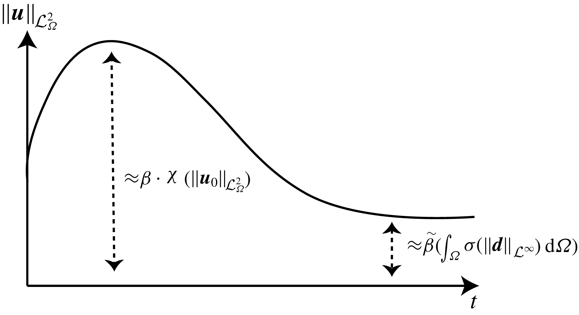
In fact, by input-to-state superposition theorem (Sontag Reference Sontag, Baillieul and Samad2013), we can show that stability to persistent disturbances is the conjunction of two properties, one of them concerned with asymptotic bounds on the perturbation velocities, in the sense of
 $\Vert \boldsymbol{u}(t,\cdot )\Vert _{{\mathcal{L}}_{\unicode[STIX]{x1D6FA}}^{2}}$
, as a function of the magnitude of the forcings, and the other one providing a transient term obtained when we ignore forcings (see figure 1).
The stability to persistent disturbances property combines transient growth (overshoot) and asymptotic behaviour.

We now demonstrate how the problem of verifying the properties in Definitions 3.1–3.3 can be cast as verifying a set of dissipation inequalities. These results, which can be derived from Ahmadi et al. (Reference Ahmadi, Valmorbida and Papachristodoulou2016, Theorem 6), allow for the extension of well-known methods for stability, input–output and optimal perturbation analysis of linear systems to the full nonlinear Navier–Stokes equations.
We begin by studying energy growth.
Theorem 3.4. Consider the perturbation model (2.4) with
 $\boldsymbol{d}\equiv 0$
and let
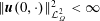 $\Vert \boldsymbol{u}(0,\cdot )\Vert _{{\mathcal{L}}_{\unicode[STIX]{x1D6FA}}^{2}}^{2}<\infty$
, i.e. the initial perturbations be square integrable over the spatial domain. If there exist a positive semi-definite storage functional
 $V(\boldsymbol{u})$
and a positive scalar
 $\unicode[STIX]{x1D6FE}$
such that
 $$\begin{eqnarray}\displaystyle & \displaystyle V(\boldsymbol{u})\leqslant \unicode[STIX]{x1D6FE}^{2}\Vert \boldsymbol{u}(t,\cdot )\Vert _{{\mathcal{L}}_{\unicode[STIX]{x1D6FA}}^{2}}^{2}, & \displaystyle\end{eqnarray}$$
 $$\begin{eqnarray}\displaystyle & \displaystyle \frac{\text{d}V(\boldsymbol{u}(t,x))}{\text{d}t}\leqslant -\int _{\unicode[STIX]{x1D6FA}}\boldsymbol{u}^{\prime }(t,x)\boldsymbol{u}(t,x)\,\text{d}\unicode[STIX]{x1D6FA}, & \displaystyle\end{eqnarray}$$
then it has bounded energy growth as given by (3.5).
The next result pertains to worst-case energy amplification.
Theorem 3.5. Consider the perturbation model (2.4) and let
 $\Vert \boldsymbol{d}(t,\cdot )\Vert _{{\mathcal{L}}_{\unicode[STIX]{x1D6FA}}^{2}}^{2}<\infty$
, i.e. the disturbances be square integrable over the spatial domain. If there exist a positive semi-definite storage functional
 $V(\boldsymbol{u})$
and positive scalars
 $\{\unicode[STIX]{x1D702}_{i}\}_{i\in I}$
such that
 $$\begin{eqnarray}\displaystyle \frac{\text{d}V(\boldsymbol{u}(t,x))}{\text{d}t}\leqslant -\int _{\unicode[STIX]{x1D6FA}}\boldsymbol{u}^{\prime }(t,x)\boldsymbol{u}(t,x)\,\text{d}\unicode[STIX]{x1D6FA}+\int _{\unicode[STIX]{x1D6FA}}\mathop{\sum }_{i\in I}\unicode[STIX]{x1D702}_{i}^{2}d_{i}^{2}(t,x)\,\text{d}\unicode[STIX]{x1D6FA}, & & \displaystyle\end{eqnarray}$$
then the perturbation velocities (2.4) have worst-case disturbance amplification upper bounds
 $\unicode[STIX]{x1D702}_{i}$
,
 $i\in I$
as in (3.6).
Lastly, we study amplifications to persistent forcings.
Theorem 3.6. Consider the perturbation model (2.4) and let
 $\Vert \boldsymbol{d}\Vert _{{\mathcal{L}}_{[0,\infty )}^{\infty }}<\infty$
, i.e. the disturbances have an upper bound. If there exist a positive semi-definite storage functional
 $V(\boldsymbol{u})$
, a positive scalar
 $\unicode[STIX]{x1D713}$
and functions
 $\unicode[STIX]{x1D6FD}_{1},\unicode[STIX]{x1D6FD}_{2},\unicode[STIX]{x1D70E}\in {\mathcal{K}}_{\infty }$
such that
 $$\begin{eqnarray}\displaystyle & \displaystyle \unicode[STIX]{x1D6FD}_{1}(\Vert \boldsymbol{u}(t,\cdot )\Vert _{{\mathcal{L}}_{\unicode[STIX]{x1D6FA}}^{2}})\leqslant V(\boldsymbol{u})\leqslant \unicode[STIX]{x1D6FD}_{2}(\Vert \boldsymbol{u}(t,\cdot )\Vert _{{\mathcal{L}}_{\unicode[STIX]{x1D6FA}}^{2}}), & \displaystyle\end{eqnarray}$$
 $$\begin{eqnarray}\displaystyle & \displaystyle \frac{\text{d}V(\boldsymbol{u}(t,x))}{\text{d}t}\leqslant -\unicode[STIX]{x1D713}V(\boldsymbol{u}(t,x))+\int _{\unicode[STIX]{x1D6FA}}\unicode[STIX]{x1D70E}(|\boldsymbol{d}(t,x)|)\,\text{d}\unicode[STIX]{x1D6FA}, & \displaystyle\end{eqnarray}$$
then the perturbation velocities described by (2.4) are stable to persistent disturbances as given by (3.8) with
 $\unicode[STIX]{x1D712}=\unicode[STIX]{x1D6FD}_{2}$
,
 $\unicode[STIX]{x1D6FD}=\unicode[STIX]{x1D6FD}_{1}^{-1}\circ 2$
and
 $\tilde{\unicode[STIX]{x1D6FD}}=\unicode[STIX]{x1D6FD}_{1}^{-1}\circ 2/\unicode[STIX]{x1D713}$
, where
 $\circ$
implies function composition.
In the following, we derive classes of storage functionals
 $V(\boldsymbol{u})$
suitable for the analysis of perturbation dynamics (2.4) invariant in one of the three spatial coordinates. We consider two classes of flows, namely channel flows with perturbations that vary in two spatial dimensions and time discussed in § 3.2 and pipe flows invariant in the axial direction discussed in appendix C.
3.2 A Lyapunov/storage functional for flows between parallel plates
In Cartesian coordinates, for a scalar function
 $v$
,
 $\unicode[STIX]{x1D735}v=\sum _{i}\unicode[STIX]{x2202}_{x_{i}}v\boldsymbol{e}_{i}$
and
 $\unicode[STIX]{x1D6FB}^{2}v=\sum _{i}\unicode[STIX]{x2202}_{x_{i}}^{2}v$
, where
 $\boldsymbol{e}_{i}$
is the unit vector in the direction
 $x_{i}$
. For a vector valued function
 $\boldsymbol{w}=\sum _{i}w_{i}\boldsymbol{e}_{i}$
, and the divergence
 $\unicode[STIX]{x1D735}\boldsymbol{\cdot }\boldsymbol{w}$
is given by
 $\unicode[STIX]{x1D735}\boldsymbol{\cdot }\boldsymbol{w}=\sum _{i}\unicode[STIX]{x2202}_{x_{i}}w_{i}$
. In the following,
 $\{x_{1},x_{2},x_{3}\}$
correspond to
 $\{x,y,z\}$
(the streamwise, wall-normal and spanwise directions) and
 $I=\{1,2,3\}$
. Additionally, we adopt Einstein’s multi-index notation over index
 $j$
, that is the sum over repeated indices
 $j$
, e.g.
 $v_{j}\unicode[STIX]{x2202}_{x_{j}}u_{i}=\sum _{j}v_{j}\unicode[STIX]{x2202}_{x_{j}}u_{i}$
.
The perturbation model (2.4) can be rewritten as
 $$\begin{eqnarray}\left.\begin{array}{@{}c@{}}\displaystyle \unicode[STIX]{x2202}_{t}u_{i}=\frac{1}{Re}\unicode[STIX]{x1D6FB}^{2}u_{i}-u_{j}\unicode[STIX]{x2202}_{x_{j}}u_{i}-U_{j}\unicode[STIX]{x2202}_{x_{j}}u_{i}-u_{j}\unicode[STIX]{x2202}_{x_{j}}U_{i}-\unicode[STIX]{x2202}_{x_{i}}p+d_{i},\\ \displaystyle 0=\unicode[STIX]{x2202}_{x_{j}}u_{j},\end{array}\right\}\end{eqnarray}$$
where
 $i,j\in I$
. To simplify the exposition, without loss of generality, we assume that the perturbations are invariant with respect to
 $x_{1}$
. Since
 $x_{i},i=1,2,3$
are arbitrary, this does not affect the formulation.
The next proposition states that, by choosing a suitable storage functional structure (weighted kinetic energy of the perturbation velocities), the time derivative of the storage functional turns out to be upper-bounded by a quadratic form in the velocity fields
 $\boldsymbol{u}$
and their spatial derivatives. This property paves the way for a convex-optimization-based method to check input–output properties. Convex optimization is a subfield of optimization that studies the problem of minimizing convex functions over convex sets. The convexity makes optimization easier than the general case since local minimum must be a global minimum, and first-order conditions are sufficient conditions for optimality (Boyd & Vandenberghe Reference Boyd and Vandenberghe2004). Convex optimization problems can be solved efficiently by interior-point methods (Nesterov & Nemirovskii Reference Nesterov and Nemirovskii1994). Convex optimization was used by Moarref et al. (Reference Moarref, Jovanovic, Tropp, Sharma and McKeon2014) to obtain a low-order decomposition of the Navier–Stokes equations based on resolvent modes.
Proposition 3.7. Consider the perturbation model (3.15) subject to periodic or no-slip boundary conditions
 $\boldsymbol{u}|_{\unicode[STIX]{x2202}\unicode[STIX]{x1D6FA}}=0$
. Assume the velocity perturbations in (3.15) are invariant with respect to
 $x_{1}$
. Let
 $I_{0}=\{2,3\}$
and
 $$\begin{eqnarray}V(\boldsymbol{u})=\frac{1}{2}\int _{\unicode[STIX]{x1D6FA}}\boldsymbol{u}^{\prime }\unicode[STIX]{x1D64C}\boldsymbol{u}\,\text{d}\unicode[STIX]{x1D6FA},\end{eqnarray}$$
where
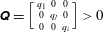 $\unicode[STIX]{x1D64C}=\Big[\begin{smallmatrix}q_{1} & 0 & 0\\ 0 & q_{j} & 0\\ 0 & 0 & q_{i}\end{smallmatrix}\Big]>0$
,
 $q_{i}=q_{j}$
for
 $i\neq j$
,
 $i,j\in I_{0}$
, be a candidate storage functional. Then, the time derivative of (3.16) along the solutions to (3.15) satisfies
 $$\begin{eqnarray}\frac{\text{d}V(\boldsymbol{u})}{\text{d}t}\leqslant -\mathop{\sum }_{i\in I}q_{i}\int _{\unicode[STIX]{x1D6FA}}\left(\frac{C}{Re}u_{i}^{2}+U_{j}u_{i}\unicode[STIX]{x2202}_{x_{j}}u_{i}+u_{j}u_{i}\unicode[STIX]{x2202}_{x_{j}}U_{i}-u_{i}d_{i}\right)\,\text{d}\unicode[STIX]{x1D6FA},\end{eqnarray}$$
where
 $C$
is a positive constant that only depends on the domain
 $\unicode[STIX]{x1D6FA}$
.
The proof of this proposition is given in appendix A.
Note that a special case of (3.16) was used in Joseph & Hung (Reference Joseph and Hung1971) to study the stability of viscous flows (subject to streamwise-constant perturbations) in pipes and between rotating cylinders. The authors referred to this structure as the two energy function. In the formulation presented in this paper, assuming invariant perturbations in the
 $x_{1}$
-direction, and since the inequalities hold if scaled by a positive scalar, we can represent the two energy function as
 $$\begin{eqnarray}V(\boldsymbol{u})=\frac{1}{2}\int _{\unicode[STIX]{x1D6FA}}\boldsymbol{u}^{\prime }\left[\begin{array}{@{}ccc@{}}q & 0 & 0\\ 0 & 1 & 0\\ 0 & 0 & 1\end{array}\right]\boldsymbol{u}\,\text{d}\unicode[STIX]{x1D6FA},\end{eqnarray}$$
where
 $q$
is a positive scalar. The ‘optimal’ value for this constant was then calculated analytically for the pipe Poiseuille and the Taylor–Couette flow by Joseph & Hung (Reference Joseph and Hung1971).
Indeed, considering streamwise-constant perturbations provides a degree of freedom in the Lyapunov/storage functional, which can be used to study flow properties at higher Reynolds numbers. When the perturbations are spatially varying in all three directions, the Lyapunov/storage functional converts to the energy functional, which has been used to study the stability of viscous flows (Serrin Reference Serrin1959). However, since for three-dimensional perturbations there is no degree of freedom in the structure of the Lyapunov/storage functional, the flow properties can only be studied for low Reynolds numbers.
Note that in (3.17) the Poincaré constant,
 $C$
, appears. There are several estimates for the optimal Poincaré constant. The optimal constant (Payne & Weinberger Reference Payne and Weinberger1960) we use in this paper is
 $$\begin{eqnarray}C(\unicode[STIX]{x1D6FA})=\frac{\unicode[STIX]{x03C0}^{2}}{D(\unicode[STIX]{x1D6FA})},\end{eqnarray}$$
where
 $D(\unicode[STIX]{x1D6FA})$
is the diameter of the domain
 $\unicode[STIX]{x1D6FA}$
(the longest distance between any two point in the domain
 $\unicode[STIX]{x1D6FA}$
).
Proposition 3.7 allows us to provide an algorithmic method for input–output analysis of fluid flows based on convex optimization. These convex optimization problems are in terms of linear matrix inequalities and polynomial matrix inequalities. This formulation is delineated in more detail in the next section.
4 Matrix inequalities for input–output analysis of streamwise-constant perturbations
In this section, we show that the input–output analysis problem outlined in § 3 for the class of streamwise-constant perturbations can be converted into a set of matrix inequalities. These matrix inequalities can be solved by convex optimization, provided that the base flow is a polynomial in the spatial coordinates and the flow geometry is described by a semi-algebraic set. (Let
 ${\mathcal{R}}[x]$
be the set of polynomials with real coefficients. A set is semi-algebraic if it can be described by a finite number of polynomial equalities and inequalities. That is,
 ${\mathcal{S}}\subset \mathbb{R}^{n}$
for some closed field, say
 $\mathbb{R}$
, is defined by a set of polynomial equalities and inequalities as
 ${\mathcal{S}}=\{x\in \mathbb{R}^{n}\mid p_{i}(x)\geqslant 0,i=1,2,\ldots ,n_{p},q_{i}(x)=0,i=1,2,\ldots ,n_{q}\}$
, where
 $\{p_{i}\}_{i=1}^{n_{p}},\{q_{i}\}_{i=1}^{n_{q}}\in {\mathcal{R}}[x]$
, where
 ${\mathcal{R}}[x]$
denotes the set of polynomials in the variable
 $x$
with real coefficients.) Examples are laminar base flows that are linear or parabolic, and turbulent flows that can be represented by polynomial fits (or by piecewise polynomial functions). (Note that by the Weierstrass approximation theorem (De Branges Reference De Branges1959), any continuous function defined on a closed interval can be uniformly approximated as closely as desired by a polynomial function.)
To present a convex method for checking the conditions in theorems 3.4–3.6 (see also corollary B.1 in appendix B), we restrict our attention to streamwise-constant perturbations in the
 $x_{1}$
-direction with base flow
 $\boldsymbol{U}=U_{m}(x_{2},x_{3})\boldsymbol{e}_{1}$
, where
 $\boldsymbol{e}_{1}$
denotes the unit vector in the
 $x_{1}$
-direction.
In order to present the procedure, we first need to define the following notation. For a square matrix
 $\unicode[STIX]{x1D648}$
,
 $\unicode[STIX]{x1D648}\succcurlyeq 0$
(
 $\unicode[STIX]{x1D648}\succ 0$
) implies that the matrix is positive semi-definite (positive definite), i.e. all the eigenvalues of
 $\unicode[STIX]{x1D648}$
are non-negative (positive). Similarly,
 $\unicode[STIX]{x1D648}\preccurlyeq 0$
(
 $\unicode[STIX]{x1D648}\prec 0$
) signifies that
 $-\unicode[STIX]{x1D648}\succcurlyeq 0$
(
 $-\unicode[STIX]{x1D648}\succ 0$
). By
 $\unicode[STIX]{x1D644}_{n\times n}$
, we denote the square matrix of dimension
 $n\times n$
with diagonal entries set to
 $1$
.
Corollary 4.1. Consider the perturbation dynamics given by (3.15), which are constant in the streamwise direction
 $x_{1}$
and with base flow
 $\boldsymbol{U}=U_{m}(x)\boldsymbol{e}_{1}$
, where
 $x=(x_{2},x_{3})$
. Let
 $I_{0}=\{2,3\}$
. If there exist positive constants
 $\{q_{l}\}_{l\in I}$
with
 $q_{i}=q_{j}$
,
 $i,j\in I_{0}$
,
 $\{\unicode[STIX]{x1D702}_{l}\}_{l\in I}$
,
 $\unicode[STIX]{x1D713}$
, and functions
 $\{\unicode[STIX]{x1D70E}_{l}\}_{l\in I}$
such that
 $$\begin{eqnarray}\unicode[STIX]{x1D648}(x)=\left[\begin{array}{@{}ccc@{}}\displaystyle \frac{C}{Re}q_{1} & \displaystyle \frac{q_{1}\unicode[STIX]{x2202}_{x_{j}}U_{m}(x)}{2} & \displaystyle \frac{q_{1}\unicode[STIX]{x2202}_{x_{i}}U_{m}(x)}{2}\\ \displaystyle \frac{q_{1}\unicode[STIX]{x2202}_{x_{j}}U_{m}(x)}{2} & \displaystyle \frac{C}{Re}q_{j} & 0\\ \displaystyle \frac{q_{1}\unicode[STIX]{x2202}_{x_{i}}U_{m}(x)}{2} & 0 & \displaystyle \frac{C}{Re}q_{i}\end{array}\right],\quad i,j\in I_{0},i\neq j,\end{eqnarray}$$
(I) when
 $\boldsymbol{d}\equiv 0$
,
 $$\begin{eqnarray}\unicode[STIX]{x1D648}(x)-\unicode[STIX]{x1D644}_{3\times 3}\succcurlyeq 0,\quad x\in \unicode[STIX]{x1D6FA},\end{eqnarray}$$
(II)

for
 $i,j\in I_{0},i\neq j$
and
 $x\in \unicode[STIX]{x1D6FA}$
,
(III)
 $\unicode[STIX]{x1D70E}_{l}(x)\geqslant 0,x\in \unicode[STIX]{x1D6FA}$
,
 $l\in I$
and

for
 $i,j\in I_{0},i\neq j$
and
 $x\in \unicode[STIX]{x1D6FA}$
, where
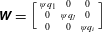 $\unicode[STIX]{x1D652}=\Big[\begin{smallmatrix}\unicode[STIX]{x1D713}q_{1} & 0 & 0\\ 0 & \unicode[STIX]{x1D713}q_{j} & 0\\ 0 & 0 & \unicode[STIX]{x1D713}q_{i}\end{smallmatrix}\Big]$
. Then, it follows that
(I) the flow energy growth is bounded by
 $\unicode[STIX]{x1D6FE}^{2}=\max _{i\in I}q_{i}$
as described by (3.5),
(II) the worst-case disturbance amplification (induced
${\mathcal{L}}^{2}$
-norm from the disturbances to perturbation velocities) is bounded by
$\unicode[STIX]{x1D702}_{i}$
,
$i\in I$
as in (3.6) when the initial perturbations have zero velocity,(III) the flow is stable to persistent disturbances in the sense of (3.8) with
$\unicode[STIX]{x1D70E}(|\boldsymbol{d}|)=\sum _{i\in I}\unicode[STIX]{x1D70E}_{i}(x)d_{i}^{2}$
.



The proof of the above corollary is given in appendix B.
When
 $U_{m}(x)$
is a polynomial function, inequalities (4.1)–(4.4) are polynomial matrix inequalities that should be checked for all
 $x\in \unicode[STIX]{x1D6FA}$
. If the set
 $\unicode[STIX]{x1D6FA}$
is a semi-algebraic set, i.e.
 $$\begin{eqnarray}\unicode[STIX]{x1D6FA}=\{x\in \mathbb{R}^{2}\mid g_{l}(x)=0,f_{k}(x)>0,l=1,2,\ldots ,L,k=1,2,\ldots ,K\},\end{eqnarray}$$
where
 $\{g_{l}\}_{l=1}^{L}$
and
 $\{f_{k}\}_{k=1}^{K}$
are polynomial functions, then these inequalities can be cast as a sum-of-squares program by applying corollary D.4. We show in the next section that this assumption is indeed the case for several well-known flows. For a brief introduction to sum-of-squares programming, refer to appendix D. Note that once the input–output analysis problem is cast as a sum-of-squares program, it can be checked using available MATLAB toolboxes such as SOSTOOLS (Papachristodoulou et al.
Reference Papachristodoulou, Anderson, Valmorbida, Prajna, Seiler and Parrilo2013) and YALMIP (Löfberg Reference Löfberg2004).
We can compute the bound on the maximum energy growth described in (3.5) by solving an optimization problem. To this end, we solve
 $$\begin{eqnarray}\left.\begin{array}{@{}c@{}}\displaystyle \underset{\{q_{i}\}_{i\in I}}{\text{minimize}}\left(\underset{i\in I}{\max }\,q_{i}\right)\\ \displaystyle \text{subject to}\\ \displaystyle \unicode[STIX]{x1D648}(x)-\unicode[STIX]{x1D644}_{3\times 3}\succcurlyeq 0,\quad \forall x\in \unicode[STIX]{x1D6FA},\\ \displaystyle q_{i}>0,\quad i\in I.\end{array}\right\}\end{eqnarray}$$
In order to find upper bounds on the worst-case disturbance amplification (the induced
 ${\mathcal{L}}^{2}$
-norm) from the body forces or disturbances
 $\boldsymbol{d}$
to the perturbation velocities
 $\boldsymbol{u}$
as described in (3.6), we solve the following optimization problem:
 $$\begin{eqnarray}\left.\begin{array}{@{}c@{}}\displaystyle \underset{\{q_{i}\}_{i\in I},\{\unicode[STIX]{x1D702}_{i}\}_{i\in I}}{\text{minimize}}\mathop{\sum }_{i\in I}\unicode[STIX]{x1D702}_{i}^{2}\\ \displaystyle \text{subject to}\\ \displaystyle \unicode[STIX]{x1D649}(x)\succcurlyeq 0,\quad \forall x\in \unicode[STIX]{x1D6FA},\\ \displaystyle \unicode[STIX]{x1D702}_{i}>0,\quad i\in I,\\ \displaystyle q_{i}>0,\quad i\in I.\end{array}\right\}\end{eqnarray}$$
5 Numerical results
In this section, we apply the proposed method to three canonical flows, namely plane Couette flow, plane Poiseuille flow and Hagen–Poiseuille flow. For each case we compute bounds on energy growth, worst-case disturbance amplification and stability to persistent forcings (i.e. ISS). Our analysis of the worst-case disturbance amplification includes a comparative analysis of the influence of each of the disturbance components. For the case of stability to persistent disturbances, we find the maximum Reynolds number for which stability to persistent disturbances holds.
For each result, we provide explicit descriptions of the matrix inequalities that need to be solved to study each of the three input–output properties based on theorems 3.4–3.6. These matrix inequalities can then be solved using available MATLAB toolboxes such as SOSTOOLS (Papachristodoulou et al. Reference Papachristodoulou, Anderson, Valmorbida, Prajna, Seiler and Parrilo2013) and YALMIP (Löfberg Reference Löfberg2004) as described in appendix D.
5.1 Plane Couette flow
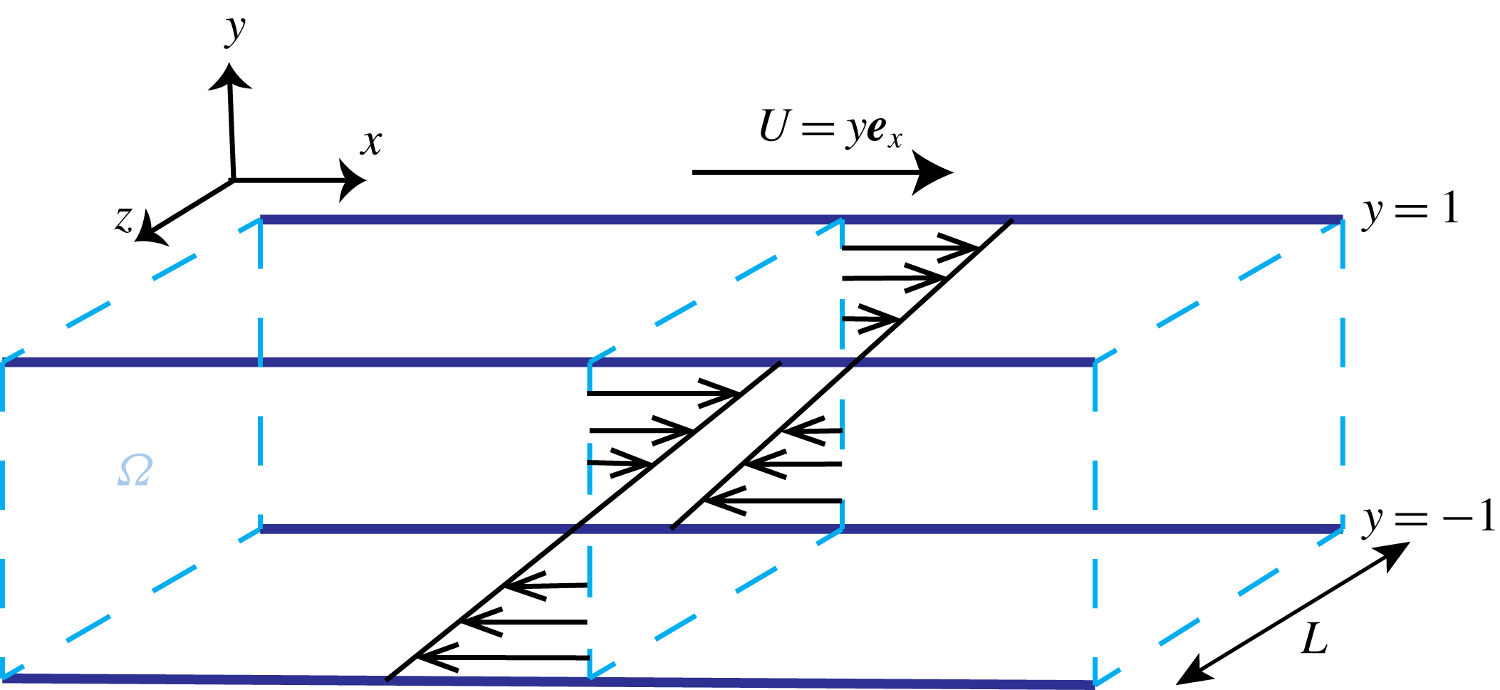
We consider the flow of viscous fluid between two parallel plates, where the gap between the plates is much smaller than the length of the plates as illustrated in figure 2. The base flow is given by
 $\boldsymbol{U}=(y,0,0)^{\prime }=y\boldsymbol{e}_{x}$
and
 $P=P_{0}$
.
Schematic of the plane Couette flow geometry.

We consider no-slip boundary conditions
 $\boldsymbol{u}|_{y=-1}^{1}=0$
in the wall-normal direction and
 $\boldsymbol{u}(t,y,z)=\boldsymbol{u}(t,y,z+L)$
in the spanwise direction. The Poincaré constant is then given by
 $C=\unicode[STIX]{x03C0}^{2}/\sqrt{L^{2}+2^{2}}$
.
A storage functional of the form (3.16) can be used to compute bounds on all three quantities of interest (i.e. energy growth, worst-case amplification and stability to persistent forcings):
 $$\begin{eqnarray}V(u)=\int _{0}^{L}\int _{-1}^{1}\left[\begin{array}{@{}c@{}}u_{x}\\ u_{y}\\ u_{z}\end{array}\right]^{\prime }\left[\begin{array}{@{}ccc@{}}q_{x} & 0 & 0\\ 0 & q_{y} & 0\\ 0 & 0 & q_{z}\end{array}\right]\left[\begin{array}{@{}c@{}}u_{x}\\ u_{y}\\ u_{z}\end{array}\right]\,\text{d}y\,\text{d}z,\end{eqnarray}$$
with
 $q_{y}=q_{z}$
.
We assume that spatial invariance in the
 $x$
-direction, and thus (
 $m=x,j=y,i=z$
). The
 $\unicode[STIX]{x1D648}$
matrix in (4.1) is then given by
 $$\begin{eqnarray}\unicode[STIX]{x1D648}=\left[\begin{array}{@{}ccc@{}}\displaystyle \frac{q_{x}C}{Re} & \displaystyle \frac{q_{x}}{2} & 0\\ \displaystyle \frac{q_{x}}{2} & \displaystyle \frac{q_{y}C}{Re} & 0\\ 0 & 0 & \displaystyle \frac{q_{y}C}{Re}\end{array}\right].\end{eqnarray}$$
Given a channel width
 $L=\unicode[STIX]{x03C0}$
we can compute the input–output energy growth by solving the optimization problem (4.5) with
 $\unicode[STIX]{x1D648}$
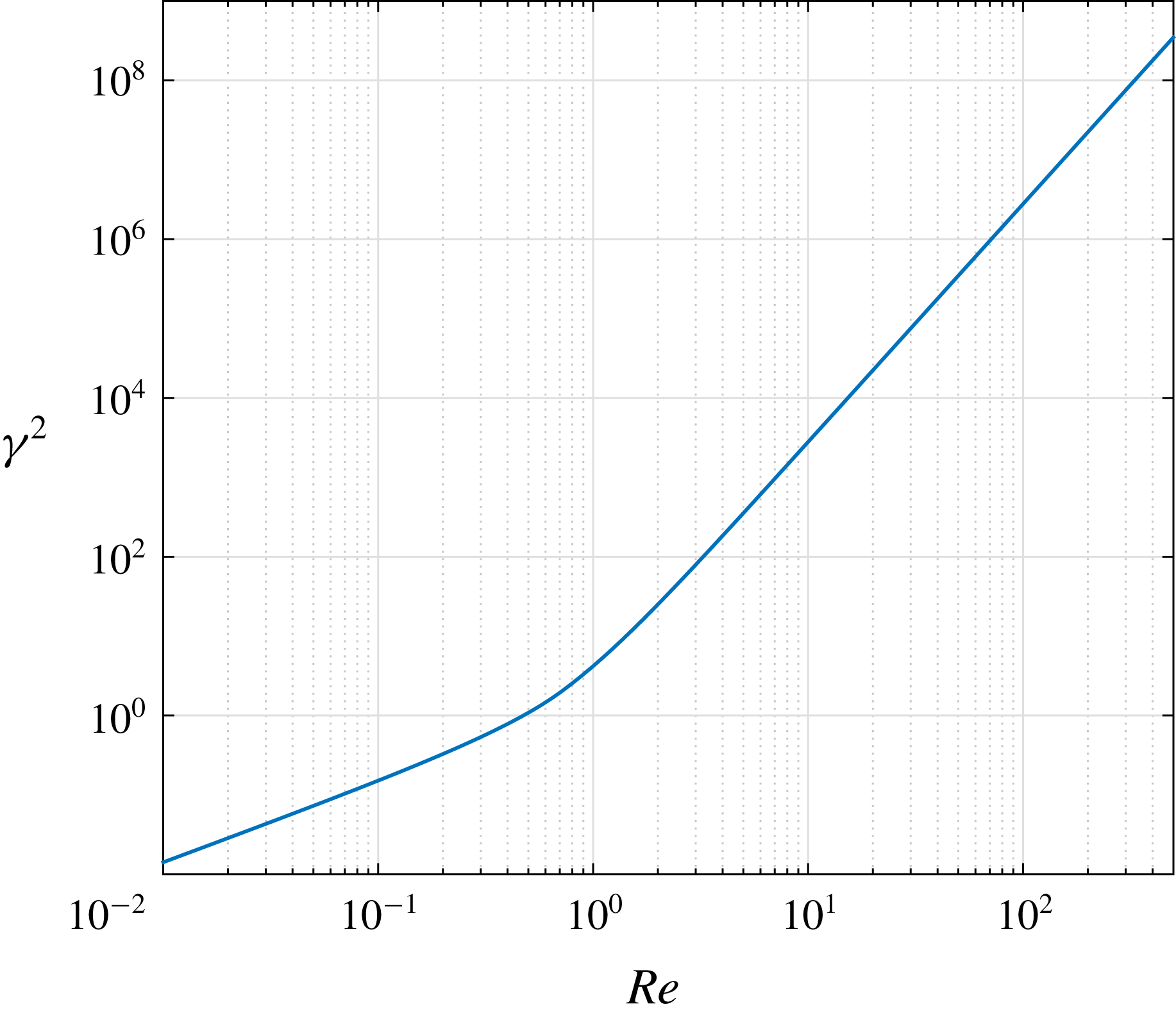
given by (5.2). The resulting energy growth
 $\unicode[STIX]{x1D6FE}^{2}$
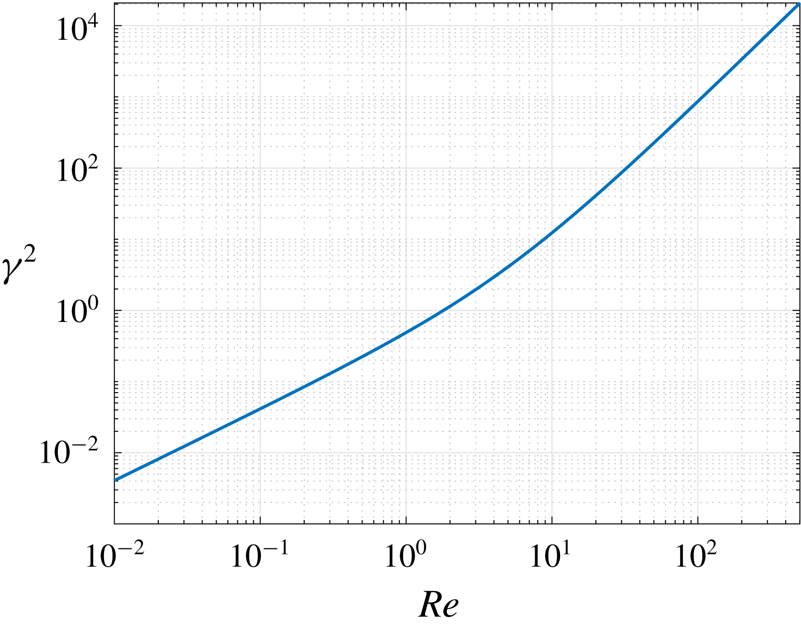
as a function of Reynolds number is plotted in figure 3. For small Reynolds numbers
 $\unicode[STIX]{x1D6FE}^{2}\sim O(Re)$
, whereas for larger Reynolds numbers
 $\unicode[STIX]{x1D6FE}^{2}\sim O(Re^{3})$
. Therefore, it can be inferred that
 $\unicode[STIX]{x1D6FE}^{2}\sim c_{0}Re+c_{1}Re^{3}$
with
 $c_{0},c_{1}>0$
. This scaling is consistent with the results obtained by Bobba, Bamieh & Doyle (Reference Bobba, Bamieh and Doyle2002), where the maximum energy growth of streamwise-constant (nonlinear) plane Couette flow was calculated analytically based on a streamwise-constant
 $(2\text{-}\text{D}/3\text{-}\text{C})$
model. It is worth noting that we calculated the scalings by interpolation of the upper bounds computed from the convex optimization problems in terms of the Reynolds numbers. In the cases for which a polynomial fit could not be found, we measured the slope of the line in the amplification versus Reynolds number plot (figure 3).
Upper bounds on the maximum energy growth for plane Couette flow in terms of Reynolds numbers.

We next compute the worst-case amplification using the matrix inequality (4.3), which for this particular flow is given by

with
 $\unicode[STIX]{x1D648}$
as in (5.2).
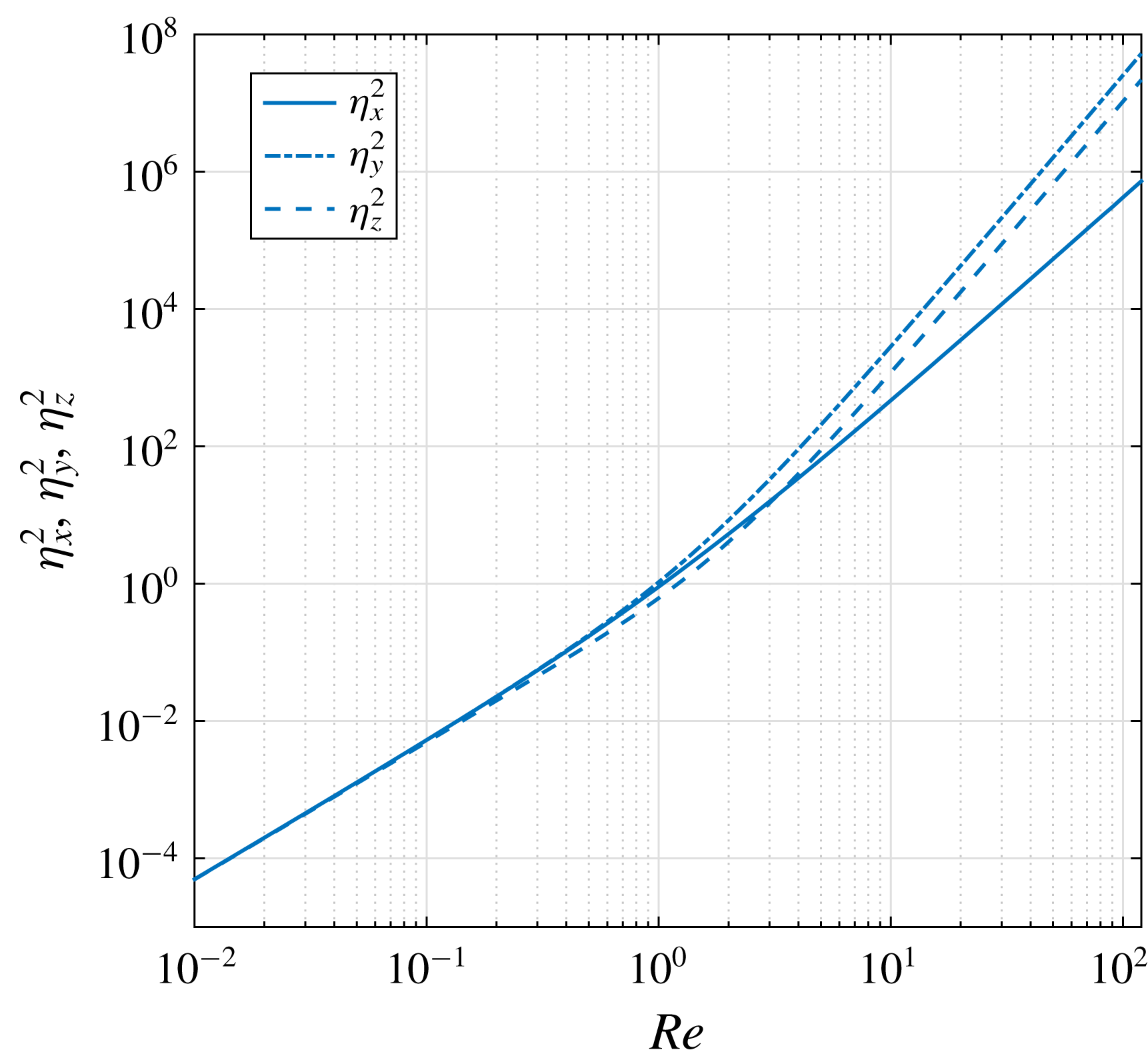
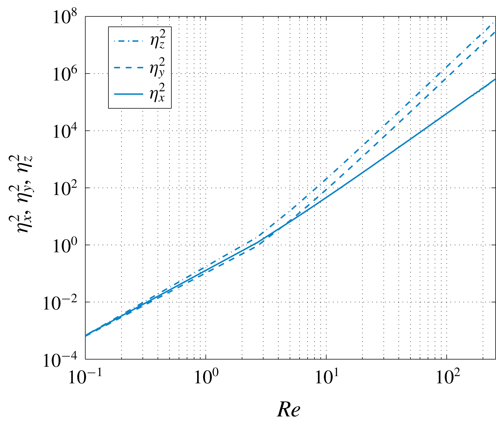
Upper bounds on the worst-case amplification for perturbation velocities of plane Couette flow for different Reynolds numbers.

The resulting upper bounds on the worst-case amplification for
 $2\text{-}\text{D}/3\text{-}\text{C}$
plane Couette flow obtained by minimizing
 $\unicode[STIX]{x1D702}_{x}^{2}$
,
 $\unicode[STIX]{x1D702}_{y}^{2}$
and
 $\unicode[STIX]{x1D702}_{z}^{2}$
are given in figure 4. Since the flow is stable for all Reynolds numbers, the worst-case amplifications are increasing monotonically with Reynolds number. The results in figure 4 imply
 $\unicode[STIX]{x1D702}_{x}^{2}\sim a_{0}Re^{2}+a_{1}Re^{3}$
,
 $\unicode[STIX]{x1D702}_{y}^{2}\sim b_{0}Re^{2}+b_{1}Re^{4}$
and
 $\unicode[STIX]{x1D702}_{z}^{2}\sim c_{0}Re^{2}+c_{1}Re^{4}$
with
 $a_{0},a_{1},b_{0},b_{1},c_{0},c_{1}>0$
. This implies that worst-case amplifications in all three components of disturbances grow with a
 $Re^{2}$
ratio for very low Reynolds numbers. For Reynolds numbers approximately greater than
 $1$
, the streamwise disturbances are amplified at a rate proportional to
 $Re^{3}$
; whereas, the wall-normal and spanwise disturbance component amplification scales as
 $Re^{4}$
.
The upper bounds depicted in figure 4 can be compared with corollary F.2 (see appendix F), wherein it was demonstrated that
 $\unicode[STIX]{x1D702}_{x}^{2}=f_{0}Re^{2}$
,
 $\unicode[STIX]{x1D702}_{y}^{2}=g_{0}Re^{2}+g_{1}Re^{4}$
and
 $\unicode[STIX]{x1D702}_{z}^{2}=h_{0}Re^{2}+h_{1}Re^{4}$
for the linearized plane Couette flow with constants
 $f_{0},g_{0},g_{1},h_{0},h_{1}>0$
by solving Lyapunov equations.
Finally, we compute the stability to persistent forcings (ISS) property using inequality (4.4) from corollary 4.1. Applying this to the
 $2\text{-}\text{D}/3\text{-}\text{C}$
Couette flow of interest leads to

with
 $\unicode[STIX]{x1D648}$
given in (5.2) and
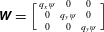 $\unicode[STIX]{x1D652}=\Bigl[\begin{smallmatrix}q_{x}\unicode[STIX]{x1D713} & 0 & 0\\ 0 & q_{y}\unicode[STIX]{x1D713} & 0\\ 0 & 0 & q_{y}\unicode[STIX]{x1D713}\end{smallmatrix}\Bigr]$
. We fix
 $\unicode[STIX]{x1D713}=10^{-4}$
and the channel width to
 $L=2\unicode[STIX]{x03C0}$
. In this case, we obtain
 $Re_{ISS}=316$
. The quantity
 $Re_{ISS}=316$
is interestingly close to the empirical transition Reynolds number
 $Re\approx 350$
obtained experimentally by Tillmark & Alfredsson (Reference Tillmark and Alfredsson1992). In this sense, it turns out that
 $Re_{ISS}$
is surprisingly close to the Reynolds number above which transition occurs. Understanding this connection is an interesting direction for future work.
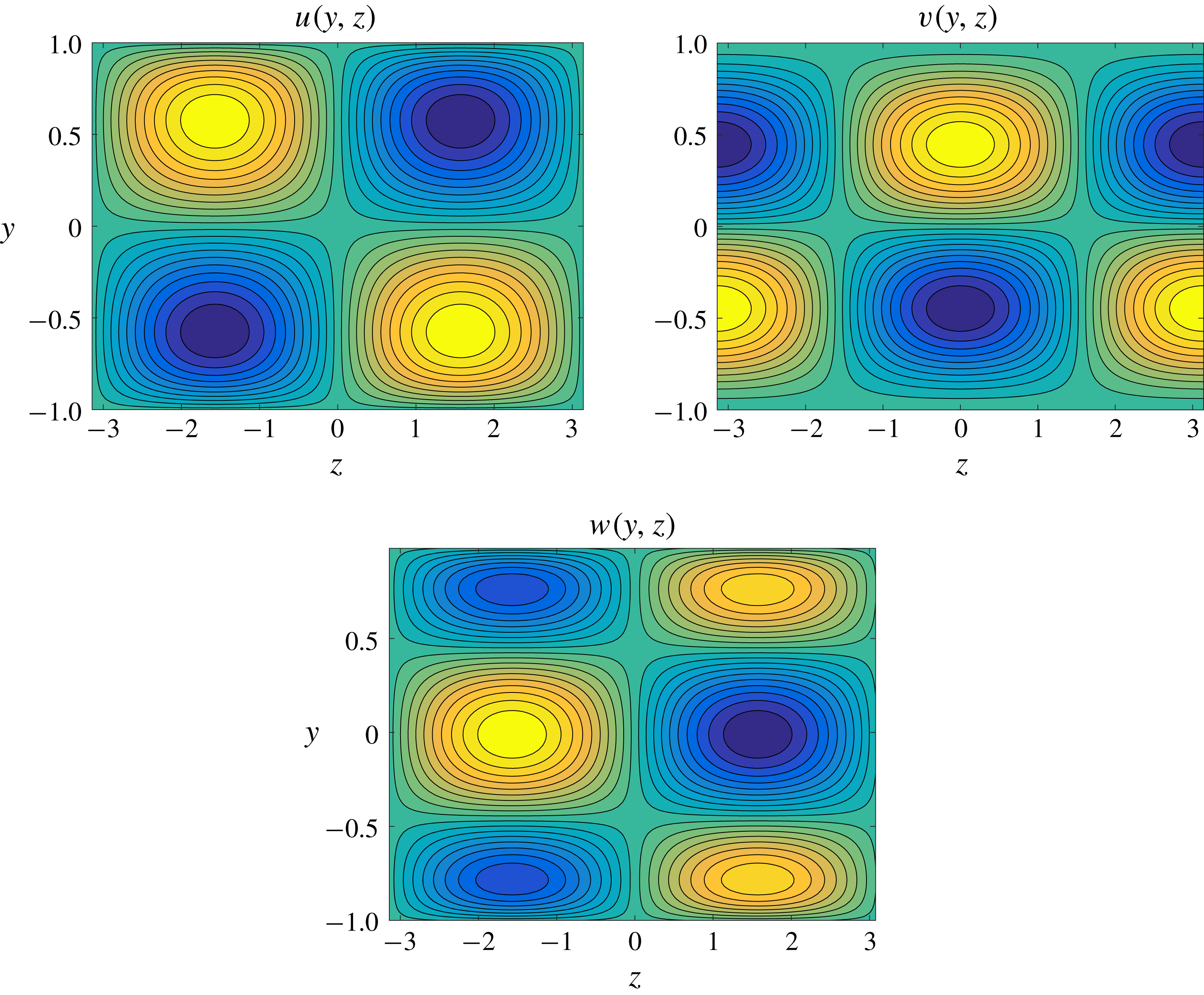
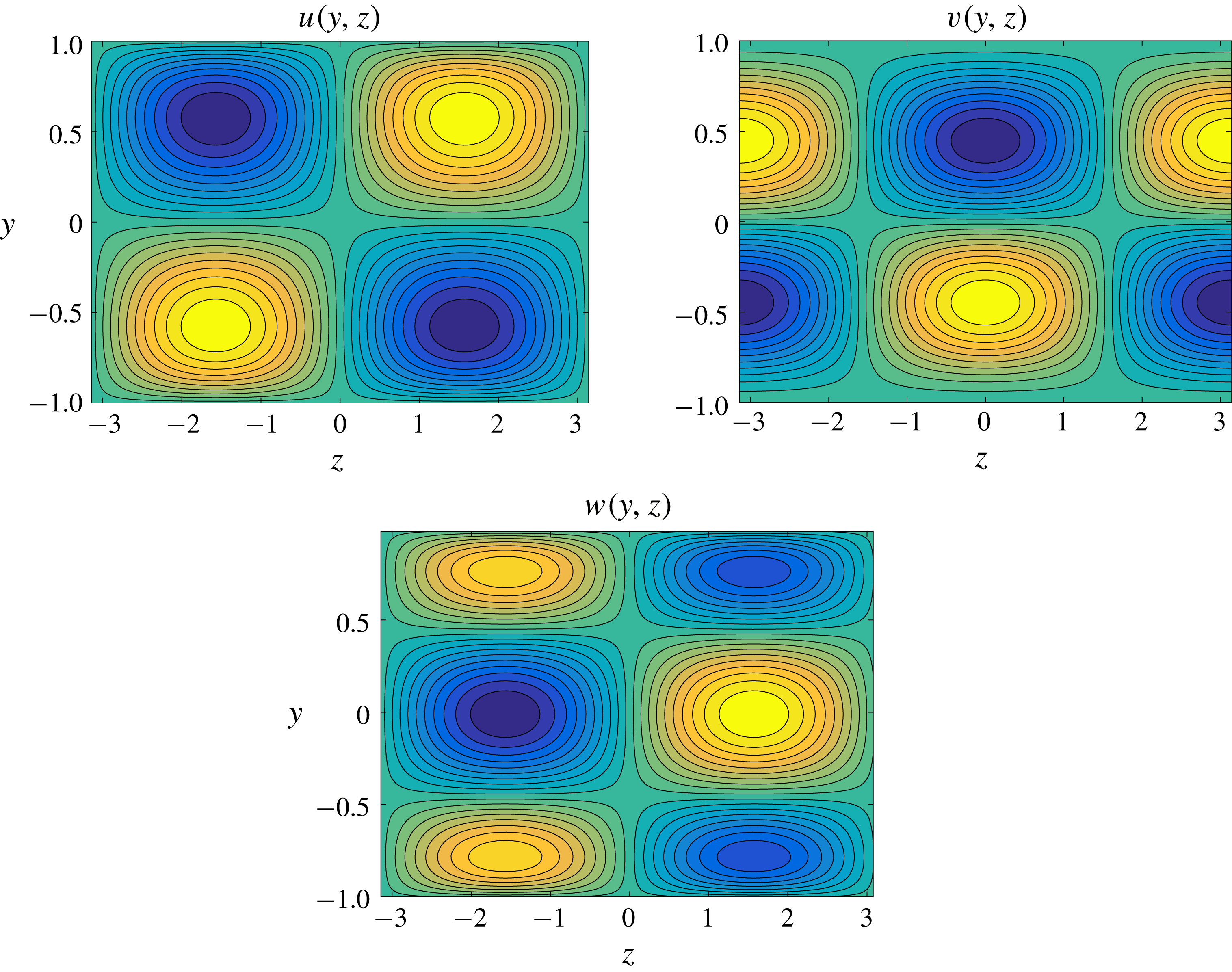
The perturbation flow structures with maximum amplification from persistent forcings at
 $Re=316$
for plane Couette flow.

In order to understand the above result on stability to persistent disturbances, we carried out numerical experiments to investigate the flow structures that receive maximum amplification from persistent disturbances. The experiments were undertaken for the linearized Navier–Stokes equation through the Orr–Sommerfeld equations. Appendix E discusses the details of these numerical experiments. Notice that these results are based on solving linear matrix inequalities that ensure stability to persistent forcings for the ODE obtained through spatial discretization of the Orr–Sommerfeld equations. Our simulations were carried out using a
 $50\times 50$
grid on the wavenumber space
 $k_{x}-k_{z}$
(
 $k_{x},k_{z}\in [0,150]$
) and the linear matrix inequalities were computed at each point in the grid. Then, the wavenumbers corresponding to the maximum amplification are selected (especially, we are interested to find
 $k_{x}$
corresponding to maximum amplification, as this is the streamwise direction) and the corresponding flow structure is simulated. As expected the maximum amplification corresponds to the streamwise-constant case
 $k_{x}=0$
. Figure 5 illustrates the flow structures that receive maximum amplification at
 $Re=316$
.
It is also worth mentioning that certificates for stability to persistent disturbances of the linearized Navier–Stokes equation, as discussed in appendix E, could be constructed for all Reynolds numbers, which is in contrast to the nonlinear case studied in this example. This illustrates that stability to persistent disturbances is a fundamentally nonlinear phenomenon.
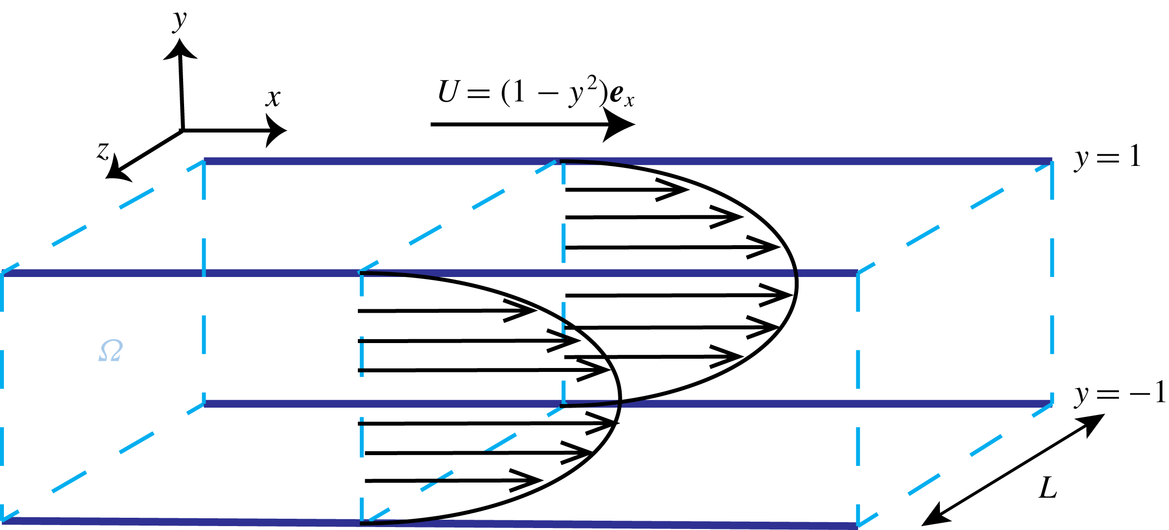
Schematic of the plane Poiseuille flow geometry.

5.2 Plane Poiseuille flow
Similar to the plane Couette flow, we consider the flow of viscous fluid between two parallel plates, where the gap between the plates is much smaller than the length of the plates. Here, the plates are stationary and the flow is induced by a pressure gradient in the flow direction. The flow geometry is depicted in figure 6.
The domain
 $\unicode[STIX]{x1D6FA}$
is defined as
 $\unicode[STIX]{x1D6FA}=\{(y,z)\mid -1<y<1,0<z<L\}$
. The base flow is given by
 $\boldsymbol{U}=U_{m}(y)\boldsymbol{e}_{x}=(1-y^{2})\boldsymbol{e}_{x}$
and
 $P=1-(4x/Re)$
. We consider no-slip boundary conditions
 $\boldsymbol{u}|_{y=-1}^{1}=0$
and
 $\boldsymbol{u}(t,y,z)=\boldsymbol{u}(t,y,z+L)$
. The Poincaré constant is then given by
 $C=\unicode[STIX]{x03C0}^{2}/\sqrt{L^{2}+2^{2}}$
.
We can again study the the input–output properties of the flow using the storage functional (5.1). For this flow, the flow perturbations are assumed invariant in the streamwise direction
 $x$
, i.e. (
 $m=x,j=y,i=z$
).
We compute the upper bounds on maximum energy growth for this flow by solving the optimization problem (4.5) with
 $$\begin{eqnarray}\unicode[STIX]{x1D648}(y)=\left[\begin{array}{@{}ccc@{}}\displaystyle \frac{q_{x}C}{Re} & -yq_{x} & 0\\ -yq_{x} & \displaystyle \frac{q_{y}C}{Re} & 0\\ 0 & 0 & \displaystyle \frac{q_{y}C}{Re}\end{array}\right].\end{eqnarray}$$
The results are illustrated in figure 7, which shows that the maximum energy amplification is described by
 $\unicode[STIX]{x1D6FE}^{2}\sim b_{0}Re+b_{1}Re^{2}$
, with
 $b_{0},b_{1}>0$
. This result is consistent with transient growth calculations of Reddy & Henningson (Reference Reddy and Henningson1993), in which the authors showed that the transient growth of the linearized plane Poiseuille flow model behaves like
 $O(Re^{2})$
for large Reynolds numbers.
For worst-case amplification analysis, we use inequality (4.3) which for this flow is given by the following matrix inequality:

with
 $\unicode[STIX]{x1D648}$
as in (5.5). By minimizing
 $\unicode[STIX]{x1D702}_{x}^{2}$
,
 $\unicode[STIX]{x1D702}_{y}^{2}$
and
 $\unicode[STIX]{x1D702}_{z}^{2}$
, we compute upper bounds on the worst-case amplification for the plane Poiseuille flow that are depicted in figure 8. From figure 8, it can be inferred that
 $\unicode[STIX]{x1D702}_{x}^{2}\sim a_{0}Re^{2}+a_{1}Re^{3}$
,
 $\unicode[STIX]{x1D702}_{y}^{2}\sim b_{0}Re^{2.2}+b_{1}Re^{4}$
and
 $\unicode[STIX]{x1D702}_{z}^{2}\sim c_{0}Re^{2}+c_{1}Re^{4}$
with
 $a_{0},a_{1},b_{0},b_{1},c_{0},c_{1}>0$
. From this result, we can infer that the worst-case amplifications in all three components of disturbances grow with a
 $Re^{2}$
ratio for low Reynolds numbers. For Reynolds numbers approximately greater than
 ${\approx}5$
, the streamwise disturbances are amplified proportional to
 $Re^{3}$
; whereas, the wall-normal and spanwise disturbance components show
 $Re^{4}$
amplification.
Upper bounds on the maximum energy growth for plane Poiseuille flow in terms of Reynolds numbers.

Upper bounds on the worst-case amplification of plane Poiseuille flow for different Reynolds numbers.

We again evaluate stability to persistent disturbances using inequality (4.4) from corollary 4.1 flow, i.e.

with
 $\unicode[STIX]{x1D648}$
given in (5.5) and
 $\unicode[STIX]{x1D652}=\left[\!\begin{smallmatrix}q_{x}\unicode[STIX]{x1D713} & 0 & 0\\ 0 & q_{y}\unicode[STIX]{x1D713} & 0\\ 0 & 0 & q_{y}\unicode[STIX]{x1D713}\end{smallmatrix}\!\right]$
. We fix
 $\unicode[STIX]{x1D713}=10^{-4}$
and
 $L=2\unicode[STIX]{x03C0}$
. In this case, we obtain
 $Re_{ISS}=1855$
. The quantity
 $Re_{ISS}=1855$
can be compared with the empirical Reynolds number at the onset of turbulence
 $Re\approx 2000$
as discussed by Grossmann (Reference Grossmann2000). Once again, we observe that
 $Re_{ISS}$
provides a bound that is consistent with the Reynolds number at which transition to turbulence occurs in channel flows, an observation that leads to some interesting future research questions that are beyond the scope of the current work.
The perturbation flow structures with maximum amplification to persistent disturbances at
 $Re=1855$
for plane Poiseuille flow.

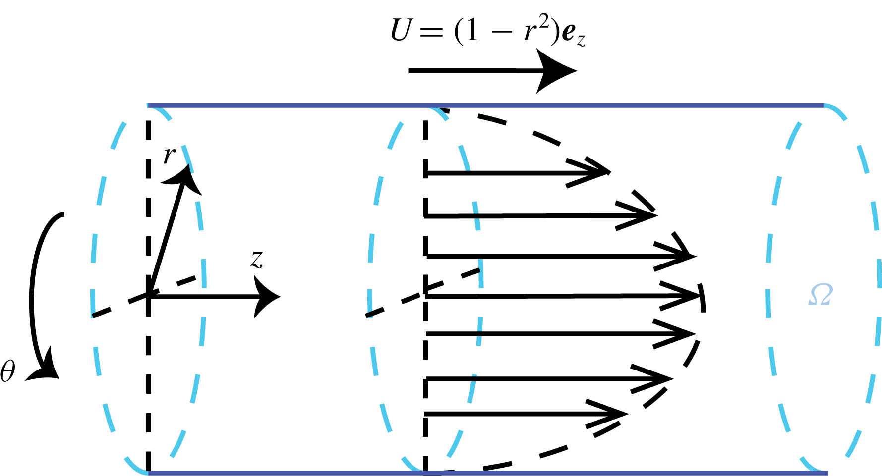
Schematic of the Hagen–Poiseuille flow geometry.

Analogous to the plane Couette flow, we undertook numerical experiments to find the flow structures subject to maximum amplification from persistent forcings. Again, we found that the maximum amplification corresponds to the streamwise-constant case
 $k_{x}=0$
. Figure 9 illustrates the flow structures that receive maximum amplification from persistent forcings at
 $Re=1855$
.
5.3 Hagen–Poiseuille flow
In this section we examine the input–output properties of Hagen–Poiseuille flow using an extension of the analysis framework that is detailed in appendix C. In particular, we consider the flow of viscous fluid driven by a pressure gradient, illustrated in figure 10. The domain
 $\unicode[STIX]{x1D6FA}$
is defined as
 $\unicode[STIX]{x1D6FA}=\{(r,\unicode[STIX]{x1D703})\mid 0<r<1,0<\unicode[STIX]{x1D703}<2\unicode[STIX]{x03C0}\}$
. The base flow is given by
 $\boldsymbol{U}=U_{m}(r)\boldsymbol{e}_{z}=(1-r^{2})\boldsymbol{e}_{z}$
and
 $P=1-4z/Re$
.
We again assume that flow is invariant in the streamwise direction
 $z$
, based on observations (e.g. Schmid & Henningson Reference Schmid and Henningson1994) that axially constant perturbations are subject to maximum background energy amplification in pipe flow. Then, the perturbation dynamics is given by (C 2) in appendix C with
 $U_{m}(r)=1-r^{2}$
. Moreover, we assume no-slip boundary conditions
 $\boldsymbol{u}|_{r=1}=0$
.
We consider the storage functional given in (C 3). Then, substituting
 $U_{m}$
and
 $F$
, we have
 $$\begin{eqnarray}\unicode[STIX]{x1D648}_{c}(r)=\left[\begin{array}{@{}ccc@{}}\displaystyle \frac{q_{z}C}{Re} & -rq_{z} & 0\\ -rq_{z} & \displaystyle \frac{q_{r}C}{Re} & 0\\ 0 & 0 & \displaystyle \frac{q_{\unicode[STIX]{x1D703}}C}{Re}\end{array}\right].\end{eqnarray}$$
Computation of the bounds on maximum energy growth in Hagen–Poiseuille flow as a function of disturbance direction and velocity component is an extension of previous analysis such as Jovanović & Bamieh (Reference Jovanović and Bamieh2005) that considered channel flows. We obtain these bounds by solving the optimization problem (4.5) with
 $\unicode[STIX]{x1D648}=\unicode[STIX]{x1D648}_{c}(r)$
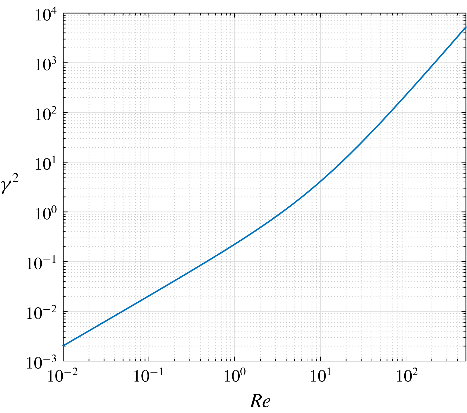
as in (5.8). The results are illustrated in figure 11. The results imply that the maximum energy growth is described by
 $\unicode[STIX]{x1D6FE}^{2}\sim b_{0}Re+b_{1}Re^{2}$
, with
 $b_{0},b_{1}>0$
. This bound is in agreement with the calculations and numerical experiments of Schmid & Henningson (Reference Schmid and Henningson1994), where the authors investigated transient growth based on the linearized Navier–Stokes equations for pipe flow.
Upper bounds on the maximum energy growth for Hagen–Poiseuille flow in terms of Reynolds numbers.

Considering
 $\unicode[STIX]{x1D648}_{c}(r)$
as in (5.8), inequality (C 14) becomes

Minimizing
 $\unicode[STIX]{x1D702}_{z}^{2}$
,
 $\unicode[STIX]{x1D702}_{r}^{2}$
and
 $\unicode[STIX]{x1D702}_{\unicode[STIX]{x1D703}}^{2}$
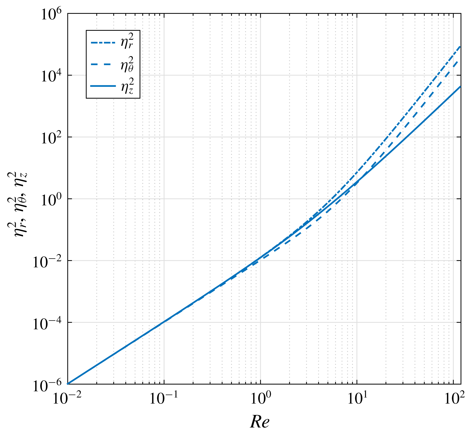
subject to the above inequality provides upper bounds on the worst-case disturbance amplification, which are plotted in figure 12 as a function of Reynolds number. Figure 12 indicates that the perturbations are amplified as
 $\unicode[STIX]{x1D702}_{z}^{2}\sim a_{0}Re^{2}+a_{1}Re^{3}$
,
 $\unicode[STIX]{x1D702}_{\unicode[STIX]{x1D703}}^{2}\sim b_{0}Re^{2}+b_{1}Re^{4}$
and
 $\unicode[STIX]{x1D702}_{r}^{2}\sim c_{0}Re^{2}+c_{1}Re^{4}$
with
 $a_{0},a_{1},b_{0},b_{1},c_{0},c_{1}>0$
. Thus, similar to channel flows, for low Reynolds numbers, the worst-case amplifications from all three disturbance components scale as
 $Re^{2}$
. For Reynolds numbers greater than
 ${\approx}8$
, the amplifications from axial (flow direction) disturbances grow proportional to
 $Re^{3}$
; whereas, the worst-case amplifications from azimuthal and radial disturbances increase as
 $Re^{4}$
.
Upper bounds on the worst-case amplification of the Hagen–Poiseuille flow in terms of different Reynolds numbers.

We compute the bounds on stability to persistent forcings using the following polynomial matrix inequality:

where
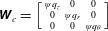 $\unicode[STIX]{x1D652}_{c}=\Big[\begin{smallmatrix}\unicode[STIX]{x1D713}q_{z} & 0 & 0\\ 0 & \unicode[STIX]{x1D713}q_{r} & 0\\ 0 & 0 & \unicode[STIX]{x1D713}q_{\unicode[STIX]{x1D703}}\end{smallmatrix}\Big]$
, which is analogous to inequality (C 15) in corollary C.2. The maximum Reynolds number for the system to remain stable to persistent forcings (i.e. remained input-to-state stable) was
 $Re_{ISS}=1614$
. Obtaining this bound required the use of degree-10 polynomials in
 $\unicode[STIX]{x1D70E}_{z}(r),\unicode[STIX]{x1D70E}_{\unicode[STIX]{x1D703}}(r)$
and
 $\unicode[STIX]{x1D70E}_{r}(r)$
. This result is again consistent with the lower bound on the Reynolds number for which transition to turbulence was observed empirically by Peixinho & Mullin (Reference Peixinho and Mullin2006), i.e.
 $Re\approx 1800$
, and provides further support that this is a connection worth investigating.
6 Discussion
We studied input–output properties of fluid flows with spatially invariant perturbations in one of the directions using dissipation inequalities. Our framework generalizes certain types of input–output analysis techniques to the nonlinear Navier–Stokes equations, thereby matching more closely with experimental results. The proposed input–output analysis method introduces a unified framework for addressing a broad range of questions related to transition (transient growth and input–output analysis) that can be adapted to a large class of flows, especially for those in which the base flow can be represented by a polynomial of spatial coordinates and the flow geometry is described by a semi-algebraic set. We showed how the input–output framework can be computationally implemented based on convex optimization. For illustration purposes, we applied the proposed method to study several examples of flows between parallel plates and pipe flow.
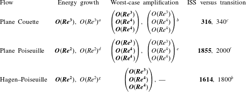
Table 1 lists the numerical results based on the proposed framework for plane Couette flow, plane Poiseuille flow and Hagen–Poiseuille flow. For energy growth and worst-case amplification, the table outlines the amplification scalings at high Reynolds numbers. Energy growth results for all three flows are consistent with the theoretical and experimental amplification scalings in the literature. Our worst-case amplification scalings for plane Couette flow and plane Poiseuille flow were similar to the scalings calculated by Bamieh & Dahleh (Reference Bamieh and Dahleh2001) and Jovanović & Bamieh (Reference Jovanović and Bamieh2005). In addition to comparing the scalings we obtained using our framework for channel flows, we carried out numerical experiments to study the worst-case amplification scalings in Hagen–Poiseuille flow. Our results indicate that, similar to channel flows, perturbations in the direction of the base flow are least amplified in Hagen–Poiseuille flow. For transition analysis, we compared the maximum Reynolds numbers for which stability to persistent disturbances could be certified to the Reynolds numbers for which transition to turbulence was observed experimentally. We made an interesting observation from the results that
 $Re_{ISS}$
is very similar to the Reynolds number for which transition to turbulence occurs in practice.
Summary of the numerical results using the proposed framework (boldfaced) and results reported in the literature.

a Bobba et al. (Reference Bobba, Bamieh and Doyle2002).
b Jovanović & Bamieh (Reference Jovanović and Bamieh2005).
c Tillmark & Alfredsson (Reference Tillmark and Alfredsson1992).
d Reddy & Henningson (Reference Reddy and Henningson1993).
e Jovanović & Bamieh (Reference Jovanović and Bamieh2005).
f Grossmann (Reference Grossmann2000).
g Schmid & Henningson (Reference Schmid and Henningson1994).
h Peixinho & Mullin (Reference Peixinho and Mullin2006).
Future research will focus on applying the framework proposed here to turbulent flows (Vassilicos Reference Vassilicos2015). In particular, we study time-averaged mechanical energy dissipation. For a channel flow of channel length
 $h$
, the mechanical energy dissipation per unit mass is given by
 $$\begin{eqnarray}\unicode[STIX]{x1D700}:=\frac{\unicode[STIX]{x1D708}^{3}}{h^{4}}\Vert \unicode[STIX]{x1D735}\boldsymbol{u}\Vert _{{\mathcal{L}}_{\unicode[STIX]{x1D6FA}}^{2}}^{2},\end{eqnarray}$$
where
 $\unicode[STIX]{x1D708}$
is the kinematic viscosity. Doering & Constantin (Reference Doering and Constantin1994) proposed a variational method for bounding this quantity based on the background flow decomposition. The method has been significantly successful in finding the time-averaged mechanical energy dissipation scaling with respect to the root-mean-square velocity
 $U$
and
 $\ell$
the longest length scale, i.e. it was shown that
 $$\begin{eqnarray}\unicode[STIX]{x1D700}\leqslant c_{1}\unicode[STIX]{x1D708}\frac{U^{2}}{\ell ^{2}}+c_{2}\frac{U^{3}}{\ell }.\end{eqnarray}$$
Also, bounds on
 $c_{1}$
and
 $c_{2}$
were obtained for different flows (Childress, Kerswell & Gilbert Reference Childress, Kerswell and Gilbert2001; Doering & Foias Reference Doering and Foias2002; Tang, Caulfield & Young Reference Tang, Caulfield and Young2004; Alexakis & Doering Reference Alexakis and Doering2006; Rollin, Dubief & Doering Reference Rollin, Dubief and Doering2011). In order to find bounds on the time-averaged mechanical energy dissipation, we can consider the following dissipation inequality:
 $$\begin{eqnarray}\frac{\text{d}V(\boldsymbol{u})}{\text{d}t}\leqslant \frac{\unicode[STIX]{x1D708}^{3}}{h^{4}}\Vert \unicode[STIX]{x1D735}\boldsymbol{u}\Vert _{{\mathcal{L}}_{\unicode[STIX]{x1D6FA}}^{2}}^{2}-C,\end{eqnarray}$$
where
 $C>0$
is a constant. Minimizing
 $C$
while searching over the storage functional
 $V(\boldsymbol{u})$
gives upper bounds on the time-averaged mechanical energy dissipation. It is worth pointing out that the solution to the dissipation inequality (6.3) was studied using the background method (Chernyshenko Reference Chernyshenko2017) for incompressible viscous flows. For the Kuramoto–Sivashinsky PDE, semi-definite programs have been used to study time-averaged mechanical energy dissipation (Goluskin & Fantuzzi Reference Goluskin and Fantuzzi2019) and a corresponding toolbox was developed (see also the application of the toolbox in analysing bounds for Rayleigh–Bérnard convection in Fantuzzi (Reference Fantuzzi2018)).
Another interesting problem for future research is identifying the regions of attraction for different flow configurations. For example, in the case of Taylor–Couette flow, after decomposing the Navier–Stokes equation about different flow states, one can search for estimates of the region of attraction inside which each flow state is stable.
In addition, input–output amplification mechanisms of turbulent flows are also an intriguing prospective research direction. In this regard, del Alamo & Jiménez (Reference del Alamo and Jiménez2006), and Pujals et al. (Reference Pujals, Garćia-Villalba, Cossu and Depardon2009), consider a non-polynomial model for turbulent mean velocity profiles and turbulent eddy viscosities. Polynomial approximations (of high degrees) of such nonlinear models fit the formulation given in this paper.
Lastly, more general storage functional structures can be considered. More specifically, given the nonlinear dynamics of the Navier–Stokes equations, one can consider the following class of storage functionals:
 $$\begin{eqnarray}V(\boldsymbol{u})=\int _{\unicode[STIX]{x1D6FA}}\left[\begin{array}{@{}c@{}}\boldsymbol{u}\\ \boldsymbol{u}^{2}\end{array}\right]^{\prime }\unicode[STIX]{x1D64C}\left[\begin{array}{@{}c@{}}\boldsymbol{u}\\ \boldsymbol{u}^{2}\end{array}\right]\,\text{d}\unicode[STIX]{x1D6FA}.\end{eqnarray}$$
However, a convex formulation using the above structure is not clear at the moment. Other structures for the storage functionals and convex methods for finding them were proposed by Gahlawat & Peet (Reference Gahlawat and Peet2017) and Shivakumar & Peet (Reference Shivakumar and Peet2018) for linear PDEs. Extension of the latter results to nonlinear PDEs can pave the way for input–output analysis of the Navier–Stokes equations using more general storage functional structures.
Appendix A. Proof of proposition 3.7
The time derivative of storage functional (3.16) along the solutions of (3.15) can be computed as
 $$\begin{eqnarray}\displaystyle \unicode[STIX]{x2202}_{t}V(\boldsymbol{u}) & = & \displaystyle \mathop{\sum }_{i\in I}\int _{\unicode[STIX]{x1D6FA}}q_{i}\left(\frac{1}{Re}u_{i}\unicode[STIX]{x1D6FB}^{2}u_{i}-u_{j}u_{i}\unicode[STIX]{x2202}_{x_{j}}u_{i}\right.\nonumber\\ \displaystyle & & \displaystyle -\left.U_{j}u_{i}\unicode[STIX]{x2202}_{x_{j}}u_{i}-u_{j}u_{i}\unicode[STIX]{x2202}_{x_{j}}U_{i}-u_{i}\unicode[STIX]{x2202}_{x_{i}}p+u_{i}d_{i}\right)\,\text{d}\unicode[STIX]{x1D6FA}.\end{eqnarray}$$
We first consider the term
 $\int _{\unicode[STIX]{x1D6FA}}q_{i}u_{j}u_{i}\unicode[STIX]{x2202}_{x_{j}}u_{i}\,\text{d}\unicode[STIX]{x1D6FA}$
. Using the boundary conditions, integration by parts and the incompressibility condition
 $\unicode[STIX]{x2202}_{x_{j}}u_{j}=0$
, we obtain
 $$\begin{eqnarray}\int _{\unicode[STIX]{x1D6FA}}q_{i}u_{j}u_{i}\unicode[STIX]{x2202}_{x_{j}}u_{i}\,\text{d}\unicode[STIX]{x1D6FA}=\frac{1}{2}\int _{\unicode[STIX]{x1D6FA}_{i}}q_{i}u_{j}u_{i}^{2}|_{\unicode[STIX]{x2202}\unicode[STIX]{x1D6FA}_{j}}\,\text{d}x_{i}-\frac{1}{2}\int _{\unicode[STIX]{x1D6FA}}q_{i}u_{i}^{2}(\unicode[STIX]{x2202}_{x_{j}}u_{j})\,\text{d}\unicode[STIX]{x1D6FA}=0.\end{eqnarray}$$
Secondly, we consider the pressure terms
 $\int _{\unicode[STIX]{x1D6FA}}q_{i}u_{i}\unicode[STIX]{x2202}_{x_{i}}p\,\text{d}\unicode[STIX]{x1D6FA}$
. Since the perturbations are assumed invariant in
 $x_{1}$
implying
 $\unicode[STIX]{x2202}_{x_{1}}p=0$
, we have
 $$\begin{eqnarray}\displaystyle & & \displaystyle \int _{\unicode[STIX]{x1D6FA}}(q_{2}u_{2}\unicode[STIX]{x2202}_{x_{2}}p+q_{3}u_{3}\unicode[STIX]{x2202}_{x_{3}}p)\,\text{d}\unicode[STIX]{x1D6FA}\nonumber\\ \displaystyle & & \displaystyle \quad =\int _{\unicode[STIX]{x1D6FA}_{3}}(q_{2}u_{2}p)|_{\unicode[STIX]{x2202}\unicode[STIX]{x1D6FA}_{2}}\,\text{d}x_{3}+\int _{\unicode[STIX]{x1D6FA}_{2}}(q_{3}u_{3}p)|_{\unicode[STIX]{x2202}\unicode[STIX]{x1D6FA}_{3}}\,\text{d}x_{2}-\int _{\unicode[STIX]{x1D6FA}}(q_{2}\unicode[STIX]{x2202}_{x_{2}}u_{2}p+q_{3}\unicode[STIX]{x2202}_{x_{3}}u_{3}p)\,\text{d}\unicode[STIX]{x1D6FA}\nonumber\\ \displaystyle & & \displaystyle \quad =-\int _{\unicode[STIX]{x1D6FA}}(q_{2}\unicode[STIX]{x2202}_{x_{2}}u_{2}+q_{3}\unicode[STIX]{x2202}_{x_{3}}u_{3})p\,\text{d}\unicode[STIX]{x1D6FA},\end{eqnarray}$$
where, in the first equality above, we use integration by parts and, in the second inequality, we use the boundary conditions. Then, since
 $q_{2}=q_{3}$
, using the incompressibility condition
 $\unicode[STIX]{x2202}_{x_{2}}u_{2}+\unicode[STIX]{x2202}_{x_{3}}u_{3}=0$
, (A 3) equals zero.
Finally, from (A 2) and (A 3), we conclude that the time derivative of the storage functional (A 1) is
 $$\begin{eqnarray}\unicode[STIX]{x2202}_{t}V(\boldsymbol{u})=\mathop{\sum }_{i\in I}\int _{\unicode[STIX]{x1D6FA}}q_{i}\left(\frac{1}{Re}u_{i}\unicode[STIX]{x1D6FB}^{2}u_{i}-U_{j}u_{i}\unicode[STIX]{x2202}_{x_{j}}u_{i}-u_{j}u_{i}\unicode[STIX]{x2202}_{x_{j}}U_{i}+u_{i}d_{i}\right)\,\text{d}\unicode[STIX]{x1D6FA}.\end{eqnarray}$$
Integrating by parts the
 $u_{i}\unicode[STIX]{x1D6FB}^{2}u_{i}$
term in (A 4) and using the boundary conditions, we get
 $$\begin{eqnarray}\unicode[STIX]{x2202}_{t}V(\boldsymbol{u})=\mathop{\sum }_{i\in I}\int _{\unicode[STIX]{x1D6FA}}q_{i}\left(\frac{-1}{Re}(\unicode[STIX]{x2202}_{x_{i}}u_{i})^{2}-U_{j}u_{i}\unicode[STIX]{x2202}_{x_{j}}u_{i}-u_{j}u_{i}\unicode[STIX]{x2202}_{x_{j}}U_{i}+u_{i}d_{i}\right)\,\text{d}\unicode[STIX]{x1D6FA}.\end{eqnarray}$$
Applying the Poincaré inequality (Payne & Weinberger Reference Payne and Weinberger1960) to (A 5), we obtain (3.17).
Appendix B. Derivation of the convex programs for channel flows
The next corollary proposes integral inequalities under which properties such as energy growth bounds, worst-case amplification and stability to persistent forcings can be inferred for the flow described by (3.15).
Corollary B.1. Consider the perturbation dynamics described by (3.15) subject to periodic or no-slip boundary conditions
 $\boldsymbol{u}|_{\unicode[STIX]{x2202}\unicode[STIX]{x1D6FA}}=0$
. Assume the velocity perturbations are constant with respect to
 $x_{1}$
. Let
 $I_{0}=\{2,3\}$
. If there exist positive constants
 $q_{i}$
,
 $i\in I$
, with
 $q_{i}=q_{j}$
,
 $i,j\in I_{0}$
, positive scalars
 $\unicode[STIX]{x1D713}$
,
 $\{\unicode[STIX]{x1D702}_{i}\}_{i\in I}$
and
 $\unicode[STIX]{x1D70E}\in {\mathcal{K}}$
such that
(I) when
 $\boldsymbol{d}\equiv 0$
,
 $$\begin{eqnarray}\mathop{\sum }_{i\in I}\int _{\unicode[STIX]{x1D6FA}}\left(\left(\frac{q_{i}C(\unicode[STIX]{x1D6FA})}{Re}-1\right)u_{i}^{2}+q_{i}U_{j}u_{i}\unicode[STIX]{x2202}_{x_{j}}u_{i}+q_{i}u_{j}u_{i}\unicode[STIX]{x2202}_{x_{j}}U_{i}\right)\,\text{d}\unicode[STIX]{x1D6FA}\geqslant 0,\end{eqnarray}$$
(II)
 $$\begin{eqnarray}\mathop{\sum }_{i\in I}\int _{\unicode[STIX]{x1D6FA}}\left(\left(\frac{q_{i}C(\unicode[STIX]{x1D6FA})}{Re}-1\right)u_{i}^{2}+q_{i}U_{j}u_{i}\unicode[STIX]{x2202}_{x_{j}}u_{i}+q_{i}u_{j}u_{i}\unicode[STIX]{x2202}_{x_{j}}U_{i}-q_{i}u_{i}d_{i}+\unicode[STIX]{x1D702}_{i}^{2}d_{i}^{2}\right)\,\text{d}\unicode[STIX]{x1D6FA}\geqslant 0,\end{eqnarray}$$
(III)
 $$\begin{eqnarray}\mathop{\sum }_{i\in I}\int _{\unicode[STIX]{x1D6FA}}\left(\left(\frac{q_{i}C(\unicode[STIX]{x1D6FA})}{Re}-\unicode[STIX]{x1D713}q_{i}\right)u_{i}^{2}+q_{i}U_{j}u_{i}\unicode[STIX]{x2202}_{x_{j}}u_{i}+q_{i}u_{j}u_{i}\unicode[STIX]{x2202}_{x_{j}}U_{i}-q_{i}u_{i}d_{i}+\unicode[STIX]{x1D70E}(|\boldsymbol{d}|)\right)\,\text{d}\unicode[STIX]{x1D6FA}\geqslant 0,\end{eqnarray}$$
then
(I) system (3.15) has bounded energy growth as described by (3.5) with
$\unicode[STIX]{x1D6FE}^{2}=\max _{i\in I}q_{i}$
;(II) under zero initial perturbations
$\boldsymbol{u}(0,x)\equiv 0$
, the worst-case amplification from disturbances to perturbation velocities is bounded by
$\unicode[STIX]{x1D702}_{i}$
,
$i\in I$
as in (3.6);(III) the perturbation velocities described by (3.15) are stable to persistent forcings in the sense of (3.8).


Proof. Each item is proven as follows.
(I) Given storage functional structure (3.16), we have
 $$\begin{eqnarray}V(\boldsymbol{u}(t,x))\leqslant \unicode[STIX]{x1D706}_{M}(\unicode[STIX]{x1D64C})\int _{\unicode[STIX]{x1D6FA}}\boldsymbol{u}^{\prime }\boldsymbol{u}\,\text{d}\unicode[STIX]{x1D6FA},\end{eqnarray}$$
where
 $\unicode[STIX]{x1D706}_{M}(\unicode[STIX]{x1D64C})$
denotes the maximum eigenvalue of
 $\unicode[STIX]{x1D64C}$
. Since
 $\unicode[STIX]{x1D64C}$
is diagonal, we have
 $\unicode[STIX]{x1D706}_{M}(\unicode[STIX]{x1D64C})=\max _{i\in I}q_{i}$
, which implies that
 $$\begin{eqnarray}V(\boldsymbol{u}(t,x))\leqslant \max _{i\in I}q_{i}\int _{\unicode[STIX]{x1D6FA}}\boldsymbol{u}^{\prime }\boldsymbol{u}\,\text{d}\unicode[STIX]{x1D6FA}.\end{eqnarray}$$
Therefore, (3.10) is satisfied with
 $\unicode[STIX]{x1D6FE}^{2}=\max _{i\in I}q_{i}$
. Rearranging terms in (B 1) yields
 $$\begin{eqnarray}-\mathop{\sum }_{i\in I}q_{i}\int _{\unicode[STIX]{x1D6FA}}\left(\frac{C(\unicode[STIX]{x1D6FA})}{Re}u_{i}^{2}+U_{j}u_{i}\unicode[STIX]{x2202}_{x_{j}}u_{i}+u_{j}u_{i}\unicode[STIX]{x2202}_{x_{j}}U_{i}\right)\,\text{d}\unicode[STIX]{x1D6FA}\leqslant \mathop{\sum }_{i\in I}\int _{\unicode[STIX]{x1D6FA}}u_{i}^{2}\,\text{d}\unicode[STIX]{x1D6FA}.\end{eqnarray}$$
Applying proposition 3.7 with
 $d\equiv 0$
, we obtain
 $$\begin{eqnarray}\frac{\text{d}V(\boldsymbol{u})}{\text{d}t}\leqslant -\mathop{\sum }_{i\in I}q_{i}\int _{\unicode[STIX]{x1D6FA}}\left(\frac{C(\unicode[STIX]{x1D6FA})}{Re}u_{i}^{2}+U_{j}u_{i}\unicode[STIX]{x2202}_{x_{j}}u_{i}+u_{j}u_{i}\unicode[STIX]{x2202}_{x_{j}}U_{i}\right)\,\text{d}\unicode[STIX]{x1D6FA}\leqslant \mathop{\sum }_{i\in I}\int _{\unicode[STIX]{x1D6FA}}u_{i}^{2}\,\text{d}\unicode[STIX]{x1D6FA}.\end{eqnarray}$$
Thus, inequality (3.11) is also satisfied. Applying theorem 3.4, we infer that the system has bounded energy growth.
(II) Rearranging terms in (B 2) yields
 $$\begin{eqnarray}\displaystyle & & \displaystyle -\mathop{\sum }_{i\in I}q_{i}\int _{\unicode[STIX]{x1D6FA}}\left(\frac{C(\unicode[STIX]{x1D6FA})}{Re}u_{i}^{2}+U_{j}u_{i}\unicode[STIX]{x2202}_{x_{j}}u_{i}+u_{j}u_{i}\unicode[STIX]{x2202}_{x_{j}}U_{i}-u_{i}d_{i}\right)\,\text{d}\unicode[STIX]{x1D6FA}\nonumber\\ \displaystyle & & \displaystyle \quad \leqslant \,-\mathop{\sum }_{i\in I}\int _{\unicode[STIX]{x1D6FA}}u_{i}^{2}\,\text{d}\unicode[STIX]{x1D6FA}+\mathop{\sum }_{i\in I}\int _{\unicode[STIX]{x1D6FA}}\unicode[STIX]{x1D702}_{i}^{2}d_{i}^{2}\,\text{d}\unicode[STIX]{x1D6FA}.\end{eqnarray}$$
Then, from (3.17) in proposition 3.7,
 $$\begin{eqnarray}\frac{\text{d}V(\boldsymbol{u})}{\text{d}t}\leqslant -\mathop{\sum }_{i\in I}q_{i}\int _{\unicode[STIX]{x1D6FA}}\left(\frac{C(\unicode[STIX]{x1D6FA})}{Re}u_{i}^{2}+U_{j}u_{i}\unicode[STIX]{x2202}_{x_{j}}u_{i}+u_{j}u_{i}\unicode[STIX]{x2202}_{x_{j}}U_{i}\right)\,\text{d}\unicode[STIX]{x1D6FA},\end{eqnarray}$$
we deduce that
 $$\begin{eqnarray}\frac{\text{d}V(\boldsymbol{u})}{\text{d}t}\leqslant -\mathop{\sum }_{i\in I}\int _{\unicode[STIX]{x1D6FA}}u_{i}^{2}\,\text{d}\unicode[STIX]{x1D6FA}+\mathop{\sum }_{i\in I}\int _{\unicode[STIX]{x1D6FA}}\unicode[STIX]{x1D702}_{i}^{2}d_{i}^{2}\,\text{d}\unicode[STIX]{x1D6FA}.\end{eqnarray}$$
From theorem 3.5, we infer that, under zero initial conditions, the perturbation velocities satisfy (3.6).
(III) Adopting (3.16) as a storage functional, we have
 $$\begin{eqnarray}\unicode[STIX]{x1D706}_{m}(\unicode[STIX]{x1D64C})\int _{\unicode[STIX]{x1D6FA}}\boldsymbol{u}^{\prime }\boldsymbol{u}\,\text{d}\unicode[STIX]{x1D6FA}\leqslant V(\boldsymbol{u}(t,x))\leqslant \unicode[STIX]{x1D706}_{M}(\unicode[STIX]{x1D64C})\int _{\unicode[STIX]{x1D6FA}}\boldsymbol{u}^{\prime }\boldsymbol{u}\,\text{d}\unicode[STIX]{x1D6FA},\end{eqnarray}$$
where
 $\unicode[STIX]{x1D706}_{m}(\unicode[STIX]{x1D64C})$
denotes the minimum eigenvalue of
 $\unicode[STIX]{x1D64C}$
. Hence, (3.13) is satisfied with
 $\unicode[STIX]{x1D6FD}_{1}(\cdot )=\min _{i\in I}q_{i}(\cdot )^{2}$
and
 $\unicode[STIX]{x1D6FD}_{2}(\cdot )=\max _{i\in I}q_{i}(\cdot )^{2}$
. Rearranging the terms in (B 3), we obtain
 $$\begin{eqnarray}\displaystyle & & \displaystyle -\mathop{\sum }_{i\in I}\int _{\unicode[STIX]{x1D6FA}}\left(\frac{q_{i}C(\unicode[STIX]{x1D6FA})}{Re}u_{i}^{2}+q_{i}U_{j}u_{i}\unicode[STIX]{x2202}_{x_{j}}u_{i}+q_{i}u_{j}u_{i}\unicode[STIX]{x2202}_{x_{j}}U_{i}-q_{i}u_{i}d_{i}\right)\,\text{d}\unicode[STIX]{x1D6FA}\nonumber\\ \displaystyle & & \displaystyle \quad \leqslant \,-\mathop{\sum }_{i\in I}\unicode[STIX]{x1D713}_{i}\int _{\unicode[STIX]{x1D6FA}}q_{i}u_{i}^{2}\,\text{d}\unicode[STIX]{x1D6FA}+\int _{\unicode[STIX]{x1D6FA}}\unicode[STIX]{x1D70E}(|\boldsymbol{d}|)\,\text{d}\unicode[STIX]{x1D6FA}.\end{eqnarray}$$
From (3.17) in proposition 3.7, it follows that
 $$\begin{eqnarray}\frac{\text{d}V(\boldsymbol{u})}{\text{d}t}\leqslant -\unicode[STIX]{x1D713}V(\boldsymbol{u})+\int _{\unicode[STIX]{x1D6FA}}\unicode[STIX]{x1D70E}(|\boldsymbol{d}|)\,\text{d}\unicode[STIX]{x1D6FA}.\end{eqnarray}$$
Then, from theorem 3.6, we infer that the perturbation velocities are stable to persistent forcings (3.8).◻
B.1 Proof of corollary 4.1
The proof is straightforward and follows from computing conditions (B 2)–(B 3) considering perturbations that are constant in
 $x_{1}$
, the base flow
 $\boldsymbol{U}=U_{m}\boldsymbol{e}_{1}$
and
 $\unicode[STIX]{x1D70E}(|\boldsymbol{d}|)=\sum _{i\in I}\unicode[STIX]{x1D70E}_{i}(x)d_{i}^{2}$
. Since the flow perturbations are constant in
 $x_{1}$
and the base flow is given by
 $\boldsymbol{U}=U_{m}\boldsymbol{e}_{1}$
, we have
 $U_{j}u_{i}\unicode[STIX]{x2202}_{x_{j}}u_{i}=0$
,
 $i\in I$
. The right-hand side of (3.17) hence changes to
 $$\begin{eqnarray}{\mathcal{A}}=\int _{\unicode[STIX]{x1D6FA}}\left(\frac{C(\unicode[STIX]{x1D6FA})}{Re}q_{i}u_{i}^{2}+\frac{C(\unicode[STIX]{x1D6FA})}{Re}q_{j}u_{j}^{2}+\frac{C(\unicode[STIX]{x1D6FA})}{Re}q_{1}u_{1}^{2}+u_{1}\unicode[STIX]{x2202}_{x_{i}}U_{m}u_{i}+u_{1}\unicode[STIX]{x2202}_{x_{j}}U_{m}u_{j}\right)\,\text{d}\unicode[STIX]{x1D6FA}\end{eqnarray}$$
for
 $i,j\in I_{0}$
,
 $i\neq j$
. Since the integrand in the above expression is quadratic in
 $u_{i}$
,
 $i\in I$
, it can be rewritten as
 $$\begin{eqnarray}{\mathcal{A}}=\int _{\unicode[STIX]{x1D6FA}}\left[\begin{array}{@{}c@{}}u_{1}\\ u_{j}\\ u_{i}\end{array}\right]^{\prime }\unicode[STIX]{x1D648}(x)\left[\begin{array}{@{}c@{}}u_{1}\\ u_{j}\\ u_{i}\end{array}\right]\,\text{d}\unicode[STIX]{x1D6FA},\end{eqnarray}$$
with
 $\unicode[STIX]{x1D648}(x)$
given in (4.1).
(I) Given storage functional structure (3.16), we have
 $$\begin{eqnarray}V(\boldsymbol{u}(t,x))\leqslant \unicode[STIX]{x1D706}_{M}(\unicode[STIX]{x1D64C})\int _{\unicode[STIX]{x1D6FA}}\boldsymbol{u}^{\prime }\boldsymbol{u}\,\text{d}\unicode[STIX]{x1D6FA},\end{eqnarray}$$
where
 $\unicode[STIX]{x1D706}_{M}(\unicode[STIX]{x1D64C})$
denotes the maximum eigenvalue of
 $\unicode[STIX]{x1D64C}$
. Since
 $\unicode[STIX]{x1D64C}$
is diagonal, we have
 $\unicode[STIX]{x1D706}_{M}(\unicode[STIX]{x1D64C})=\max _{i\in I}q_{i}$
. Therefore, (3.10) is satisfied with
 $\unicode[STIX]{x1D6FE}^{2}=\max _{i\in I}q_{i}$
. Rearranging terms in (B 1) yields
 $$\begin{eqnarray}-\mathop{\sum }_{i\in I}q_{i}\int _{\unicode[STIX]{x1D6FA}}\left(\frac{C(\unicode[STIX]{x1D6FA})}{Re}u_{i}^{2}+U_{j}u_{i}\unicode[STIX]{x2202}_{x_{j}}u_{i}+u_{j}u_{i}\unicode[STIX]{x2202}_{x_{j}}U_{i}\right)\,\text{d}\unicode[STIX]{x1D6FA}\leqslant \mathop{\sum }_{i\in I}\int _{\unicode[STIX]{x1D6FA}}u_{i}^{2}\,\text{d}\unicode[STIX]{x1D6FA}.\end{eqnarray}$$
Applying proposition 3.7 with
 $d\equiv 0$
, we obtain
 $$\begin{eqnarray}\frac{\text{d}V(\boldsymbol{u})}{\text{d}t}\leqslant \mathop{\sum }_{i\in I}\int _{\unicode[STIX]{x1D6FA}}u_{i}^{2}\,\text{d}\unicode[STIX]{x1D6FA}.\end{eqnarray}$$
Thus, inequality (3.11) is also satisfied. Applying theorem 3.4, we infer that the system has bounded energy growth.
(II) Inequality (B 2) is changed to
 $$\begin{eqnarray}\displaystyle & & \displaystyle {\mathcal{A}}+\int _{\unicode[STIX]{x1D6FA}}(q_{i}u_{i}d_{i}+q_{j}u_{j}d_{j}+q_{1}u_{1}d_{1})\,\text{d}\unicode[STIX]{x1D6FA}-\int _{\unicode[STIX]{x1D6FA}}(u_{i}^{2}+u_{j}^{2}+u_{1}^{2})\,\text{d}\unicode[STIX]{x1D6FA}\nonumber\\ \displaystyle & & \displaystyle \quad +\,\int _{\unicode[STIX]{x1D6FA}}(\unicode[STIX]{x1D702}_{i}^{2}d_{i}^{2}+\unicode[STIX]{x1D702}_{j}^{2}d_{j}^{2}+\unicode[STIX]{x1D702}_{1}^{2}d_{1}^{2})\,\text{d}\unicode[STIX]{x1D6FA}\geqslant 0,\end{eqnarray}$$
for
 $i,j\in I_{0}$
,
 $i\neq j$
. Moving all the terms under one integral gives
 $$\begin{eqnarray}{\mathcal{A}}+\int _{\unicode[STIX]{x1D6FA}}(q_{i}u_{i}d_{i}+q_{j}u_{j}d_{j}+q_{1}u_{1}d_{1}-u_{i}^{2}-u_{j}^{2}-u_{1}^{2}+\unicode[STIX]{x1D702}_{i}^{2}d_{i}^{2}+\unicode[STIX]{x1D702}_{j}^{2}d_{j}^{2}+\unicode[STIX]{x1D702}_{1}^{2}d_{1}^{2})\,\text{d}\unicode[STIX]{x1D6FA}\geqslant 0.\end{eqnarray}$$
Since the integrand in the above expression is quadratic in the case of
 $u_{i}$
and
 $d_{i}$
, it can be rewritten as
 $$\begin{eqnarray}\int _{\unicode[STIX]{x1D6FA}}\left[\begin{array}{@{}c@{}}u_{1}\\ u_{j}\\ u_{i}\\ d_{1}\\ d_{j}\\ d_{i}\end{array}\right]^{\prime }\unicode[STIX]{x1D649}(x)\left[\begin{array}{@{}c@{}}u_{1}\\ u_{j}\\ u_{i}\\ d_{1}\\ d_{j}\\ d_{i}\end{array}\right]\,\text{d}\unicode[STIX]{x1D6FA}\geqslant 0,\end{eqnarray}$$
where
 $\unicode[STIX]{x1D649}$
is defined in (4.3). Consequently, if (4.3) is satisfied for all
 $x\in \unicode[STIX]{x1D6FA}$
, (B 21) holds and from item II in corollary B.1 we infer that, subject to zero initial conditions, the worst-case amplification from disturbances to perturbation velocities is bounded by
 $\unicode[STIX]{x1D702}_{i}$
,
 $i\in I$
as in (3.6).
(III) The proof follows the same lines as the proof of item II above.
Appendix C. Pipe flows: cylindrical coordinates
In this appendix, we extend the proposed method to flows in cylindrical coordinates
 $(r,\unicode[STIX]{x1D703},z)$
. In cylindrical coordinates, the gradient and Laplacian operators are, respectively, defined as
 $\unicode[STIX]{x1D735}_{c}(\cdot )=\unicode[STIX]{x2202}_{r}(\cdot )\boldsymbol{e}_{r}+(1/r)\unicode[STIX]{x2202}_{\unicode[STIX]{x1D703}}(\cdot )\boldsymbol{e}_{\unicode[STIX]{x1D703}}+\unicode[STIX]{x2202}_{z}(\cdot )\boldsymbol{e}_{z}$
and
 $\unicode[STIX]{x1D6FB}_{c}^{2}(\cdot )=(1/r)\unicode[STIX]{x2202}_{r}(r\unicode[STIX]{x2202}_{r}(\cdot ))+(1/r^{2})\unicode[STIX]{x2202}_{\unicode[STIX]{x1D703}}^{2}(\cdot )+\unicode[STIX]{x2202}_{z}^{2}(\cdot )$
. The Navier–Stokes equations in cylindrical coordinates are then given by
 $$\begin{eqnarray}\left.\begin{array}{@{}c@{}}\displaystyle \unicode[STIX]{x2202}_{t}\bar{u}_{r}=\frac{1}{Re}\left(\unicode[STIX]{x1D6FB}_{c}^{2}\bar{u}_{r}-\frac{\bar{u}_{r}}{r^{2}}-\frac{2}{r^{2}}\unicode[STIX]{x2202}_{\unicode[STIX]{x1D703}}\bar{u}_{\unicode[STIX]{x1D703}}\right)-\bar{\boldsymbol{u}}\boldsymbol{\cdot }\unicode[STIX]{x1D735}_{c}\bar{u}_{r}+\frac{\bar{u}_{\unicode[STIX]{x1D703}}^{2}}{r}-\unicode[STIX]{x2202}_{r}\bar{p}+d_{r},\\ \displaystyle \unicode[STIX]{x2202}_{t}\bar{u}_{\unicode[STIX]{x1D703}}=\frac{1}{Re}\left(\unicode[STIX]{x1D6FB}_{c}^{2}\bar{u}_{\unicode[STIX]{x1D703}}-\frac{\bar{u}_{\unicode[STIX]{x1D703}}}{r^{2}}+\frac{2}{r^{2}}\unicode[STIX]{x2202}_{\unicode[STIX]{x1D703}}\bar{u}_{r}\right)-\bar{\boldsymbol{u}}\boldsymbol{\cdot }\unicode[STIX]{x1D735}_{c}\bar{u}_{\unicode[STIX]{x1D703}}-\frac{\bar{u}_{\unicode[STIX]{x1D703}}\bar{u}_{r}}{r}-\frac{1}{r}\unicode[STIX]{x2202}_{\unicode[STIX]{x1D703}}\bar{p}+d_{\unicode[STIX]{x1D703}},\\ \displaystyle \unicode[STIX]{x2202}_{t}\bar{u}_{z}=\frac{1}{Re}\unicode[STIX]{x1D6FB}_{c}^{2}\bar{u}_{z}-\bar{\boldsymbol{u}}\boldsymbol{\cdot }\unicode[STIX]{x1D735}_{c}\bar{u}_{z}-\unicode[STIX]{x2202}_{z}\bar{p}+d_{z},\\ \displaystyle 0=\frac{1}{r}\unicode[STIX]{x2202}_{r}(r\bar{u}_{r})+\frac{1}{r}\unicode[STIX]{x2202}_{\unicode[STIX]{x1D703}}\bar{u}_{\unicode[STIX]{x1D703}}+\unicode[STIX]{x2202}_{z}\bar{u}_{z},\end{array}\right\}\end{eqnarray}$$
where
 $\bar{\boldsymbol{u}}=(\bar{u}_{r},\bar{u}_{\unicode[STIX]{x1D703}},\bar{u}_{z})^{\prime }$
.
We consider the flow perturbations that are invariant in the axial direction (
 $z$
-direction). The base flow is given by
 $\boldsymbol{U}=U_{m}(r,\unicode[STIX]{x1D703})\boldsymbol{e}_{z}$
and
 $P$
. For such flows, substituting
 $\bar{\boldsymbol{u}}=\boldsymbol{u}+\boldsymbol{U}$
and
 $\bar{p}=P+p$
in (C 1), the perturbation dynamics is obtained as
 $$\begin{eqnarray}\left.\begin{array}{@{}c@{}}\displaystyle \unicode[STIX]{x2202}_{t}u_{r}=\frac{1}{Re}\unicode[STIX]{x1D6FB}_{c}^{2}u_{r}-u_{r}\unicode[STIX]{x2202}_{r}u_{r}-\frac{u_{\unicode[STIX]{x1D703}}\unicode[STIX]{x2202}_{\unicode[STIX]{x1D703}}u_{r}}{r}+\frac{u_{\unicode[STIX]{x1D703}}^{2}}{r}-\frac{u_{r}}{r^{2}Re}-\frac{2\unicode[STIX]{x2202}_{\unicode[STIX]{x1D703}}u_{\unicode[STIX]{x1D703}}}{r^{2}Re}-\unicode[STIX]{x2202}_{r}p+d_{r},\\ \displaystyle \unicode[STIX]{x2202}_{t}u_{\unicode[STIX]{x1D703}}=\frac{1}{Re}\unicode[STIX]{x1D6FB}_{c}^{2}u_{\unicode[STIX]{x1D703}}-u_{r}\unicode[STIX]{x2202}_{r}u_{\unicode[STIX]{x1D703}}-\frac{u_{\unicode[STIX]{x1D703}}\unicode[STIX]{x2202}_{\unicode[STIX]{x1D703}}u_{\unicode[STIX]{x1D703}}}{r}-\frac{u_{r}u_{\unicode[STIX]{x1D703}}}{r}-\frac{u_{\unicode[STIX]{x1D703}}}{r^{2}Re}-\frac{2\unicode[STIX]{x2202}_{\unicode[STIX]{x1D703}}u_{\unicode[STIX]{x1D703}}}{r^{2}Re}-\frac{1}{r}\unicode[STIX]{x2202}_{\unicode[STIX]{x1D703}}p+d_{\unicode[STIX]{x1D703}},\\ \displaystyle \unicode[STIX]{x2202}_{t}u_{z}=\frac{1}{Re}\unicode[STIX]{x1D6FB}_{c}^{2}u_{z}-u_{r}\unicode[STIX]{x2202}_{r}u_{z}-u_{r}\unicode[STIX]{x2202}_{r}U_{m}-\frac{u_{\unicode[STIX]{x1D703}}\unicode[STIX]{x2202}_{\unicode[STIX]{x1D703}}U_{m}}{r}-\frac{u_{\unicode[STIX]{x1D703}}\unicode[STIX]{x2202}_{\unicode[STIX]{x1D703}}u_{z}}{r}+d_{z},\\ \displaystyle 0=\unicode[STIX]{x2202}_{r}(ru_{r})+\unicode[STIX]{x2202}_{\unicode[STIX]{x1D703}}u_{\unicode[STIX]{x1D703}},\end{array}\right\}\end{eqnarray}$$
wherein
 $\boldsymbol{u}=(u_{r},u_{\unicode[STIX]{x1D703}},u_{z})^{\prime }$
.
Proposition C.1. Consider the perturbation dynamics in cylindrical coordinates (C 2) with periodic or no-slip boundary conditions
 $u\mid _{\unicode[STIX]{x2202}\unicode[STIX]{x1D6FA}}=0$
. The time derivative of storage functional
 $$\begin{eqnarray}V(\boldsymbol{u})=\frac{1}{2}\int _{\unicode[STIX]{x1D6FA}}\left[\begin{array}{@{}c@{}}u_{r}\\ u_{\unicode[STIX]{x1D703}}\\ u_{z}\end{array}\right]^{\prime }\left[\begin{array}{@{}ccc@{}}q_{r} & 0 & 0\\ 0 & q_{\unicode[STIX]{x1D703}} & 0\\ 0 & 0 & q_{z}\end{array}\right]\left[\begin{array}{@{}c@{}}u_{r}\\ u_{\unicode[STIX]{x1D703}}\\ u_{z}\end{array}\right]r\,\text{d}r\,\text{d}\unicode[STIX]{x1D703},\end{eqnarray}$$
with
 $q_{r}=q_{\unicode[STIX]{x1D703}}$
, satisfies
 $$\begin{eqnarray}\displaystyle \frac{\text{d}V(\boldsymbol{u})}{\text{d}t} & {\leqslant} & \displaystyle -\int _{\unicode[STIX]{x1D6FA}}\left(\frac{q_{r}C}{Re}u_{r}^{2}+q_{z}\unicode[STIX]{x2202}_{r}U_{m}u_{r}u_{z}+\frac{q_{z}C}{Re}u_{z}^{2}+\frac{q_{z}}{r}\unicode[STIX]{x2202}_{\unicode[STIX]{x1D703}}U_{m}u_{\unicode[STIX]{x1D703}}u_{z}+\frac{q_{\unicode[STIX]{x1D703}}C}{Re}u_{\unicode[STIX]{x1D703}}^{2}\right.\nonumber\\ \displaystyle & & \displaystyle \quad -\left.q_{r}u_{r}d_{r}-q_{\unicode[STIX]{x1D703}}u_{\unicode[STIX]{x1D703}}d_{\unicode[STIX]{x1D703}}-q_{z}u_{z}d_{z}\right)r\,\text{d}r\,\text{d}\unicode[STIX]{x1D703},\end{eqnarray}$$
where
 $C>0$
.
Proof. The time derivative of the storage functional (C 3) is given by
 $$\begin{eqnarray}\displaystyle \frac{\text{d}V(\boldsymbol{u})}{\text{d}t} & = & \displaystyle \int _{\unicode[STIX]{x1D6FA}}\left(-rq_{r}u_{r}^{2}\unicode[STIX]{x2202}_{r}u_{r}-q_{r}u_{r}u_{\unicode[STIX]{x1D703}}\unicode[STIX]{x2202}_{\unicode[STIX]{x1D703}}u_{r}+q_{r}u_{r}u_{\unicode[STIX]{x1D703}}^{2}-rq_{r}\unicode[STIX]{x2202}_{r}pu_{r}\right.\nonumber\\ \displaystyle & & \displaystyle +\left.\frac{q_{r}}{Re}ru_{r}\unicode[STIX]{x1D6FB}_{c}^{2}u_{r}-\frac{q_{r}u_{r}^{2}}{Rer}-\frac{2q_{r}u_{r}\unicode[STIX]{x2202}_{\unicode[STIX]{x1D703}}u_{\unicode[STIX]{x1D703}}}{rRe}+q_{r}ru_{r}d_{r}\right)\,\text{d}\unicode[STIX]{x1D703}\,\text{d}r\nonumber\\ \displaystyle & & \displaystyle +\,\int _{\unicode[STIX]{x1D6FA}}\left(-rq_{\unicode[STIX]{x1D703}}u_{r}u_{\unicode[STIX]{x1D703}}\unicode[STIX]{x2202}_{r}u_{\unicode[STIX]{x1D703}}-q_{\unicode[STIX]{x1D703}}u_{r}u_{\unicode[STIX]{x1D703}}\unicode[STIX]{x2202}_{\unicode[STIX]{x1D703}}u_{r}-q_{\unicode[STIX]{x1D703}}u_{r}u_{\unicode[STIX]{x1D703}}^{2}-q_{\unicode[STIX]{x1D703}}\unicode[STIX]{x2202}_{\unicode[STIX]{x1D703}}pu_{\unicode[STIX]{x1D703}}\right.\nonumber\\ \displaystyle & & \displaystyle +\left.\frac{q_{\unicode[STIX]{x1D703}}}{Re}ru_{\unicode[STIX]{x1D703}}\unicode[STIX]{x1D6FB}_{c}^{2}u_{\unicode[STIX]{x1D703}}-\frac{q_{\unicode[STIX]{x1D703}}u_{\unicode[STIX]{x1D703}}^{2}}{rRe}+\frac{2q_{\unicode[STIX]{x1D703}}\unicode[STIX]{x2202}_{\unicode[STIX]{x1D703}}u_{r}u_{\unicode[STIX]{x1D703}}}{rRe}+q_{\unicode[STIX]{x1D703}}ru_{\unicode[STIX]{x1D703}}d_{\unicode[STIX]{x1D703}}\right)\,\text{d}r\,\text{d}\unicode[STIX]{x1D703}\nonumber\\ \displaystyle & & \displaystyle +\,\int _{\unicode[STIX]{x1D6FA}}\left(-rq_{z}u_{r}u_{z}\unicode[STIX]{x2202}_{r}u_{z}-rq_{z}u_{r}u_{z}\unicode[STIX]{x2202}_{r}U_{m}-q_{z}\unicode[STIX]{x2202}_{\unicode[STIX]{x1D703}}U_{m}u_{\unicode[STIX]{x1D703}}u_{z}-q_{z}u_{\unicode[STIX]{x1D703}}u_{z}\unicode[STIX]{x2202}_{r}u_{z}\right.\nonumber\\ \displaystyle & & \displaystyle +\left.\frac{q_{z}}{Re}ru_{z}\unicode[STIX]{x1D6FB}_{c}^{2}u_{z}+q_{z}ru_{z}d_{z}\right)\,\text{d}r\,\text{d}\unicode[STIX]{x1D703}.\end{eqnarray}$$
We first focus on the terms involving pressure
 $p$
on the right-hand side of (C 5). From the incompressibility condition
 $\unicode[STIX]{x2202}_{r}(ru_{r})+\unicode[STIX]{x2202}_{\unicode[STIX]{x1D703}}u_{\unicode[STIX]{x1D703}}=0$
and the fact that
 $q_{r}=q_{\unicode[STIX]{x1D703}}$
, we obtain
 $$\begin{eqnarray}\displaystyle \int _{\unicode[STIX]{x1D6FA}}(-rq_{r}\unicode[STIX]{x2202}_{r}pu_{r}-q_{\unicode[STIX]{x1D703}}\unicode[STIX]{x2202}_{\unicode[STIX]{x1D703}}pu_{\unicode[STIX]{x1D703}})\,\text{d}r\,\text{d}\unicode[STIX]{x1D703} & = & \displaystyle \int _{\unicode[STIX]{x1D6FA}}(q_{r}\unicode[STIX]{x2202}_{r}(ru_{r})p+q_{\unicode[STIX]{x1D703}}\unicode[STIX]{x2202}_{\unicode[STIX]{x1D703}}up)\,\text{d}r\,\text{d}\unicode[STIX]{x1D703}\nonumber\\ \displaystyle & = & \displaystyle \int _{\unicode[STIX]{x1D6FA}}q_{r}p(\unicode[STIX]{x2202}_{r}(ru_{r})+\unicode[STIX]{x2202}_{\unicode[STIX]{x1D703}}u)\,\text{d}r\,\text{d}\unicode[STIX]{x1D703}=0,\end{eqnarray}$$
where, in the first equality above, we used integration by parts and the boundary conditions. At this point, we consider the other terms. Using integration by parts, boundary conditions and the incompressibility condition, it can be shown that
 $$\begin{eqnarray}\left.\begin{array}{@{}c@{}}\displaystyle \int _{\unicode[STIX]{x1D6FA}}(-rq_{r}u_{r}^{2}\unicode[STIX]{x2202}_{r}u_{r}-q_{r}u_{r}u_{\unicode[STIX]{x1D703}}\unicode[STIX]{x2202}_{\unicode[STIX]{x1D703}}u_{r})\,\text{d}r\,\text{d}\unicode[STIX]{x1D703}=\int _{\unicode[STIX]{x1D6FA}}\left(\frac{q_{r}u_{r}^{2}}{2}\unicode[STIX]{x2202}_{r}(ru_{r})+\frac{q_{r}u_{r}^{2}}{2}\unicode[STIX]{x2202}_{\unicode[STIX]{x1D703}}u_{\unicode[STIX]{x1D703}}\right)\,\text{d}r\,\text{d}\unicode[STIX]{x1D703}=0,\\ \displaystyle \int _{\unicode[STIX]{x1D6FA}}(-rq_{\unicode[STIX]{x1D703}}u_{r}u_{\unicode[STIX]{x1D703}}\unicode[STIX]{x2202}_{r}u_{\unicode[STIX]{x1D703}}-q_{\unicode[STIX]{x1D703}}u_{\unicode[STIX]{x1D703}}^{2}\unicode[STIX]{x2202}_{\unicode[STIX]{x1D703}}u_{\unicode[STIX]{x1D703}})\,\text{d}r\,d\unicode[STIX]{x1D703}=\int _{\unicode[STIX]{x1D6FA}}\left(\frac{q_{\unicode[STIX]{x1D703}}u_{\unicode[STIX]{x1D703}}^{2}}{2}\unicode[STIX]{x2202}_{r}(ru_{r})+\frac{q_{\unicode[STIX]{x1D703}}u_{\unicode[STIX]{x1D703}}^{2}}{2}\unicode[STIX]{x2202}_{\unicode[STIX]{x1D703}}u_{\unicode[STIX]{x1D703}}\right)\,\text{d}r\,\text{d}\unicode[STIX]{x1D703}=0,\\ \displaystyle \int _{\unicode[STIX]{x1D6FA}}(-rq_{z}u_{r}u_{z}\unicode[STIX]{x2202}_{r}u_{z}-q_{z}u_{\unicode[STIX]{x1D703}}u_{z}\unicode[STIX]{x2202}_{\unicode[STIX]{x1D703}}u_{z})\,\text{d}r\,\text{d}\unicode[STIX]{x1D703}=\int _{\unicode[STIX]{x1D6FA}}\left(\frac{q_{z}u_{z}^{2}}{2}\unicode[STIX]{x2202}_{r}(ru_{r})+\frac{q_{z}u_{z}^{2}}{2}\unicode[STIX]{x2202}_{\unicode[STIX]{x1D703}}u_{\unicode[STIX]{x1D703}}\right)\,\text{d}r\,\text{d}\unicode[STIX]{x1D703}=0,\end{array}\right\}\end{eqnarray}$$
and
 $$\begin{eqnarray}\int _{\unicode[STIX]{x1D6FA}}\left(-\frac{2q_{r}u_{r}\unicode[STIX]{x2202}_{\unicode[STIX]{x1D703}}u_{\unicode[STIX]{x1D703}}}{rRe}-\frac{2q_{\unicode[STIX]{x1D703}}\unicode[STIX]{x2202}_{\unicode[STIX]{x1D703}}u_{r}u_{\unicode[STIX]{x1D703}}}{rRe}\right)\,\text{d}r\,\text{d}\unicode[STIX]{x1D703}=\int _{\unicode[STIX]{x1D6FA}}\frac{2q_{r}}{rRe}(-u_{r}\unicode[STIX]{x2202}_{\unicode[STIX]{x1D703}}u_{\unicode[STIX]{x1D703}}+u_{r}\unicode[STIX]{x2202}_{\unicode[STIX]{x1D703}}u_{\unicode[STIX]{x1D703}})\,\text{d}r\,\text{d}\unicode[STIX]{x1D703}=0.\end{eqnarray}$$
Then, the time derivative expression (C 5) simplifies to
 $$\begin{eqnarray}\displaystyle \frac{\text{d}V(\boldsymbol{u})}{\text{d}t} & = & \displaystyle \int _{\unicode[STIX]{x1D6FA}}\left(\frac{q_{r}}{Re}ru_{r}\unicode[STIX]{x1D6FB}_{c}^{2}u_{r}-\frac{q_{r}u_{r}^{2}}{Rer}+q_{r}ru_{r}d_{r}\right)\,\text{d}\unicode[STIX]{x1D703}\,\text{d}r\nonumber\\ \displaystyle & & \displaystyle +\,\int _{\unicode[STIX]{x1D6FA}}\left(\frac{q_{\unicode[STIX]{x1D703}}}{Re}ru_{\unicode[STIX]{x1D703}}\unicode[STIX]{x1D6FB}_{c}^{2}u_{\unicode[STIX]{x1D703}}-\frac{q_{\unicode[STIX]{x1D703}}u_{\unicode[STIX]{x1D703}}^{2}}{rRe}+q_{\unicode[STIX]{x1D703}}ru_{\unicode[STIX]{x1D703}}d_{\unicode[STIX]{x1D703}}\right)\,\text{d}r\,\text{d}\unicode[STIX]{x1D703}\nonumber\\ \displaystyle & & \displaystyle +\,\int _{\unicode[STIX]{x1D6FA}}\left(-rq_{z}u_{r}u_{z}\unicode[STIX]{x2202}_{r}U_{m}-q_{z}\unicode[STIX]{x2202}_{\unicode[STIX]{x1D703}}U_{m}u_{\unicode[STIX]{x1D703}}u_{z}+\frac{q_{z}}{Re}ru_{z}\unicode[STIX]{x1D6FB}_{c}^{2}u_{z}+q_{z}ru_{z}d_{z}\right)\,\text{d}r\,\text{d}\unicode[STIX]{x1D703}.\qquad\end{eqnarray}$$
Factoring out
 $r$
yields
 $$\begin{eqnarray}\displaystyle & & \displaystyle \frac{\text{d}V(\boldsymbol{u})}{\text{d}t}=\int _{\unicode[STIX]{x1D6FA}}\left(\frac{q_{r}}{Re}u_{r}\unicode[STIX]{x1D6FB}_{c}^{2}u_{r}-\frac{q_{r}u_{r}^{2}}{r^{2}Re}+q_{r}u_{r}d_{r}\right)r\,\text{d}\unicode[STIX]{x1D703}\,\text{d}r\nonumber\\ \displaystyle & & \displaystyle \quad +\,\int _{\unicode[STIX]{x1D6FA}}\left(\frac{q_{\unicode[STIX]{x1D703}}}{Re}u_{\unicode[STIX]{x1D703}}\unicode[STIX]{x1D6FB}_{c}^{2}u_{\unicode[STIX]{x1D703}}-\frac{q_{\unicode[STIX]{x1D703}}u_{\unicode[STIX]{x1D703}}^{2}}{r^{2}Re}+q_{\unicode[STIX]{x1D703}}u_{\unicode[STIX]{x1D703}}d_{\unicode[STIX]{x1D703}}\right)r\,\text{d}r\,\text{d}\unicode[STIX]{x1D703}\nonumber\\ \displaystyle & & \displaystyle \quad +\,\int _{\unicode[STIX]{x1D6FA}}\left(-q_{z}u_{r}u_{z}\unicode[STIX]{x2202}_{r}U_{m}-\frac{q_{z}}{r}\unicode[STIX]{x2202}_{\unicode[STIX]{x1D703}}U_{m}u_{\unicode[STIX]{x1D703}}u_{z}+\frac{q_{z}}{Re}u_{z}\unicode[STIX]{x1D6FB}_{c}^{2}u_{z}+q_{z}u_{z}d_{z}\right)r\,\text{d}r\,\text{d}\unicode[STIX]{x1D703}.\end{eqnarray}$$
Since the terms
 $(q_{r}u_{r}^{2})/(r^{2}Re)$
and
 $(q_{\unicode[STIX]{x1D703}}u_{\unicode[STIX]{x1D703}}^{2})/(r^{2}Re)$
are non-negative, it follows that
 $$\begin{eqnarray}\displaystyle \frac{\text{d}V(\boldsymbol{u})}{\text{d}t} & {\leqslant} & \displaystyle \int _{\unicode[STIX]{x1D6FA}}\left(\frac{q_{r}}{Re}u_{r}\unicode[STIX]{x1D6FB}_{c}^{2}u_{r}+\frac{q_{\unicode[STIX]{x1D703}}}{Re}u_{\unicode[STIX]{x1D703}}\unicode[STIX]{x1D6FB}_{c}^{2}u_{\unicode[STIX]{x1D703}}+\frac{q_{z}}{Re}u_{z}\unicode[STIX]{x1D6FB}_{c}^{2}u_{z}-q_{z}u_{r}u_{z}\unicode[STIX]{x2202}_{r}U_{m}-\frac{q_{z}}{r}\unicode[STIX]{x2202}_{\unicode[STIX]{x1D703}}U_{m}u_{\unicode[STIX]{x1D703}}u_{z}\right.\nonumber\\ \displaystyle & & \displaystyle -\left.q_{r}u_{r}d_{r}-q_{\unicode[STIX]{x1D703}}u_{\unicode[STIX]{x1D703}}d_{\unicode[STIX]{x1D703}}-q_{z}u_{z}d_{z}\right)r\,\text{d}r\,\text{d}\unicode[STIX]{x1D703}\nonumber\\ \displaystyle & = & \displaystyle -\int _{\unicode[STIX]{x1D6FA}}\left(\frac{q_{r}}{Re}|\unicode[STIX]{x1D735}_{c}u_{r}|^{2}+\frac{q_{\unicode[STIX]{x1D703}}}{Re}|\unicode[STIX]{x1D735}_{c}u_{\unicode[STIX]{x1D703}}|^{2}+\frac{q_{z}}{Re}|\unicode[STIX]{x1D735}_{c}u_{z}|^{2}+q_{z}u_{r}u_{z}\unicode[STIX]{x2202}_{r}U_{m}+\frac{q_{z}}{r}\unicode[STIX]{x2202}_{\unicode[STIX]{x1D703}}U_{m}u_{\unicode[STIX]{x1D703}}u_{z}\right.\nonumber\\ \displaystyle & & \displaystyle -\left.q_{r}u_{r}d_{r}-q_{\unicode[STIX]{x1D703}}u_{\unicode[STIX]{x1D703}}d_{\unicode[STIX]{x1D703}}-q_{z}u_{z}d_{z}\right)r\,\text{d}r\,\text{d}\unicode[STIX]{x1D703},\end{eqnarray}$$
where in the last equality above integration by parts and the boundary conditions were used. Applying the Poincaré inequality (Payne & Weinberger Reference Payne and Weinberger1960), we obtain (C 4).◻
C.1 Convex formulation: pipe flows
Similar to the case of channel flows, in the following, we propose a convex formulation for pipe flows. The method relies on inequality (C 4). Note that for cylindrical coordinates
 $I=\{r,\unicode[STIX]{x1D703},z\}$
and
 $I_{0}=\{r,\unicode[STIX]{x1D703}\}$
.
Corollary C.2. Consider the perturbation dynamics given by (C 2), streamwise-constant in the
 $z$
-direction with base flow
 $\boldsymbol{U}=U_{m}(r,\unicode[STIX]{x1D703})\boldsymbol{e}_{z}$
. Suppose that there exist positive constants
 $\{q_{l}\}_{l\in I}$
with
 $q_{r}=q_{\unicode[STIX]{x1D703}}$
,
 $\unicode[STIX]{x1D713}$
, and functions
 $\{\unicode[STIX]{x1D70E}_{l}\}_{l\in I}$
such that
 $$\begin{eqnarray}\unicode[STIX]{x1D648}_{c}(r,\unicode[STIX]{x1D703})=\left[\begin{array}{@{}ccc@{}}\displaystyle \frac{C}{Re}q_{z} & \displaystyle \frac{1}{2}q_{z}\unicode[STIX]{x2202}_{r}U_{m} & \displaystyle \frac{q_{z}}{2}\frac{\unicode[STIX]{x2202}_{\unicode[STIX]{x1D703}}U_{m}}{r}\\ \displaystyle \frac{1}{2}q_{z}\unicode[STIX]{x2202}_{r}U_{m} & \displaystyle \frac{C}{Re}q_{r} & 0\\ \displaystyle \frac{q_{z}}{2}\frac{\unicode[STIX]{x2202}_{\unicode[STIX]{x1D703}}U_{m}}{r} & 0 & \displaystyle \frac{C}{Re}q_{\unicode[STIX]{x1D703}}\end{array}\right],\end{eqnarray}$$
(I)
 $$\begin{eqnarray}\unicode[STIX]{x1D648}_{c}(r,\unicode[STIX]{x1D703})-\unicode[STIX]{x1D644}_{3\times 3}\geqslant 0,\quad (r,\unicode[STIX]{x1D703})\in \unicode[STIX]{x1D6FA},\end{eqnarray}$$
(II)

(III)
 $\unicode[STIX]{x1D70E}_{l}(r,\unicode[STIX]{x1D703})\geqslant 0,(r,\unicode[STIX]{x1D703})\in \unicode[STIX]{x1D6FA}$
,
 $l\in I$
and

where
 $\unicode[STIX]{x1D652}_{c}=\Big[\begin{smallmatrix}\unicode[STIX]{x1D713}q_{z} & 0 & 0\\ 0 & \unicode[STIX]{x1D713}q_{r} & 0\\ 0 & 0 & \unicode[STIX]{x1D713}q_{\unicode[STIX]{x1D703}}\end{smallmatrix}\Big]$
. Then, it follows that
(I) the flow has bounded energy growth
$\unicode[STIX]{x1D6FE}^{2}=\max (q_{r},q_{\unicode[STIX]{x1D703}},q_{z})$
as given by (3.5),(II) subject to zero initial conditions, the induced
${\mathcal{L}}^{2}$
-norm from inputs to perturbation velocities is bounded,(III) the perturbation velocities are ISS in the sense of (3.8) with
$\unicode[STIX]{x1D70E}(|\boldsymbol{d}|)=\sum _{l\in I}\unicode[STIX]{x1D70E}_{l}(r,\unicode[STIX]{x1D703})d_{l}^{2}$
.



Note that, depending on
 $\unicode[STIX]{x2202}_{\unicode[STIX]{x1D703}}U_{m}$
,
 $\unicode[STIX]{x1D648}_{c}$
and therefore
 $\unicode[STIX]{x1D649}_{c}$
and
 $\unicode[STIX]{x1D655}_{c}$
can be functions of
 $1/r$
. Then, inequalities (C 12)–(C 15) become intractable. To circumvent this problem, since
 $r$
is positive, we can multiply (C 12)–(C 15) by positive powers of
 $r$
making the resulting inequalities solvable by convex optimization methods.
Appendix D. Polynomial optimization and sum-of-squares programming
Let
 ${\mathcal{R}}[x]$
denote the set of polynomials in
 $x$
with real coefficients and
 $\unicode[STIX]{x1D6F4}[x]\subset {\mathcal{R}}[x]$
the set of such polynomials with a sum-of-squares decomposition. We employ sum-of-squares programming in our computational formulations whenever
 $\unicode[STIX]{x1D735}\boldsymbol{U}$
depends on the spatial variables for channel flows (one exception in the plane Couette flow) and for all pipe flows. That is, we convert different input–output analysis problems into a sum-of-squares program, i.e. an optimization problem involving a linear objective function subject to a set of polynomial constraints:
 $$\begin{eqnarray}\left.\begin{array}{@{}c@{}}\displaystyle \underset{c\in \mathbb{R}^{N}}{\text{minimize}}\quad w^{\prime }c\\ \displaystyle \text{subject to}\\ \displaystyle a_{0,j}(x)+\mathop{\sum }_{i=1}^{N}p_{i}(x)a_{i,j}(x)=0,\quad j=1,2,\ldots ,\bar{J},\\ \displaystyle a_{0,j}(x)+\mathop{\sum }_{i=1}^{N}p_{i}(x)a_{i,j}(x)\in \unicode[STIX]{x1D6F4}[x],\quad j=\bar{J}+1,\bar{J}+2,\ldots ,J,\end{array}\right\}\end{eqnarray}$$
where
 $w\in \mathbb{R}^{N}$
is a vector of weighting coefficients,
 $c\in \mathbb{R}^{N}$
is a vector formed of the (unknown) coefficients of
 $\{p_{i}\}_{i=1}^{\bar{N}}\in {\mathcal{R}}[x]$
and
 $\{p_{i}\}_{i=\bar{N}+1}^{N}\in \unicode[STIX]{x1D6F4}[x]$
,
 $a_{i,j}(x)\in {\mathcal{R}}[x]$
are given scalar constant coefficient polynomials and
 $p_{i}(x)\in \unicode[STIX]{x1D6F4}[x]$
are sum-of-squares polynomial variables.
The main idea behind sum-of-squares programming is that checking whether a polynomial is positive can be relaxed into checking whether it has a sum-of-squares decomposition. Formally, if there exists a sum-of-squares decomposition for
 $p(x)\in {\mathcal{R}}[x]$
, i.e. if there exist polynomials
 $f_{1}(s),\ldots ,f_{m}(x)\in {\mathcal{R}}[x]$
such that
 $$\begin{eqnarray}p(x)=\mathop{\sum }_{i=1}^{m}f_{i}^{2}(x),\end{eqnarray}$$
then it follows that
 $p(x)$
is non-negative. Unfortunately, the converse does not hold in general; that is, there exist non-negative polynomials which do not have a sum-of-squares decomposition. (Exceptions (Reznick Reference Reznick2000): univariate polynomials of any even degree; quadratic polynomials in any number of variables; quartic polynomials in two variables.) An example of this class of non-negative polynomials is the Motzkin polynomial (Motzkin Reference Motzkin1965) given by
 $$\begin{eqnarray}p(x)=1-3x_{1}^{2}x_{2}^{2}+x_{1}^{2}x_{2}^{4}+x_{1}^{4}x_{2}^{2},\end{eqnarray}$$
which is non-negative for all
 $x\in \mathbb{R}^{2}$
but is not a sum of squares. This imposes some degree of conservatism when utilizing methods based on sum of squares. Generally, determining whether a given polynomial is positive is an NP-hard problem (Bovet & Crescenzi Reference Bovet and Crescenzi1994) (except for degrees less than four); but, sum-of-squares decompositions provide a conservative, yet computationally feasible method for checking non-negativity. The next lemma gives an intriguing formulation to the sum-of-squares decomposition problem.
Lemma D.1 (Choi, Lam & Reznick Reference Choi, Lam and Reznick1995).
A polynomial
 $p(x)$
of degree
 $2d$
belongs to
 $\unicode[STIX]{x1D6F4}[x]$
if and only if there exist a positive semi-definite matrix
 $\unicode[STIX]{x1D64C}$
(known as the Gram matrix) and a vector of monomials
 $\unicode[STIX]{x1D655}(x)$
which contains all monomial of
 $x$
of degree
 ${\leqslant}d$
such that
 $p(x)=\unicode[STIX]{x1D655}^{T}(x)\unicode[STIX]{x1D64C}\unicode[STIX]{x1D655}(x)$
.
For instance, consider the polynomial
 $$\begin{eqnarray}p(x_{1},x_{2})=5x_{1}^{4}+2x_{2}^{2}-x_{1}^{2}x_{2}^{2}-2x_{1}^{3}x_{2}-2x_{1}x_{2}^{3}.\end{eqnarray}$$
Factoring out the monomials in
 $p$
as
 $\unicode[STIX]{x1D655}(x_{1},x_{2})=(x_{1}^{2},x_{2}^{2},x_{1}x_{2})^{\prime }$
, we have
 $$\begin{eqnarray}p(x_{1},x_{2})=\left[\begin{array}{@{}c@{}}x_{1}^{2}\\ x_{2}^{2}\\ x_{1}x_{2}\end{array}\right]^{\prime }\left[\begin{array}{@{}ccc@{}}q_{11} & q_{12} & q_{13}\\ q_{21} & q_{22} & q_{23}\\ q_{31} & q_{32} & q_{33}\end{array}\right]\left[\begin{array}{@{}c@{}}x_{1}^{2}\\ x_{2}^{2}\\ x_{1}x_{2}\end{array}\right]=\unicode[STIX]{x1D655}^{T}(x)\unicode[STIX]{x1D64C}\unicode[STIX]{x1D655}(x).\end{eqnarray}$$
Then, by comparison, we have
 $q_{11}=5$
,
 $q_{22}=2$
,
 $2q_{12}+q_{33}=-1$
,
 $q_{13}=-1$
and
 $q_{23}=-1$
. If we can find a
 $\unicode[STIX]{x1D64C}\succcurlyeq 0$
, then
 $p(x_{1},x_{2})$
is positive semi-definite.
In Chesi et al. (Reference Chesi, Tesi, Vicino and Genesio1999) and Parrilo (Reference Parrilo2000) it was demonstrated that the answer to the query that whether a given polynomial
 $p(x)$
is sum of squares or not can be investigated via semi-definite programming methodologies.
Lemma D.2 (Parrilo Reference Parrilo2000).
Given a finite set
 $\{p_{i}\}_{i=0}^{m}\in {\mathcal{R}}[x]$
, the existence of a set of scalars
 $\{a_{i}\}_{i=1}^{m}\in \mathbb{R}$
such that
 $$\begin{eqnarray}p_{0}+\mathop{\sum }_{i=1}^{m}a_{i}p_{i}\in \unicode[STIX]{x1D6F4}[x]\end{eqnarray}$$
is a linear matrix inequality (LMI) feasibility problem. (An LMI is an expression of the form
 $A_{0}+x_{1}A_{1}+x_{2}A_{2}+\cdots +x_{m}A_{m}\geqslant 0,$
where
 $x\in \mathbb{R}^{m}$
and
 $A_{i}\in \mathbb{S}^{n},i=1,2,\ldots ,m$
(symmetric
 $n\times n$
matrices). An LMI specifies a convex constraint on the variables
 $x$
.)
Furthermore, we often need to verify whether a matrix with polynomial entries is positive (semi-)definite. To this end, we use the next lemma from Prajna, Papachristodoulou & Wu (Reference Prajna, Papachristodoulou and Wu2004).
Lemma D.3 (Prajna et al. Reference Prajna, Papachristodoulou and Wu2004).
Denote by
 $\otimes$
the Kronecker product. Suppose
 $F(x)\in {\mathcal{R}}^{n\times n}[x]$
is symmetric and of degree
 $2d$
for all
 $x\in \mathbb{R}^{n}$
. In addition, let
 $\unicode[STIX]{x1D655}(x)\in {\mathcal{R}}^{n\times 1}[x]$
be a column vector of monomials of degree no greater than
 $d$
and consider the following conditions:
(A)
$F(x)\geqslant 0$
for all
$x\in \mathbb{R}^{n}$
,(B)
$v^{T}F(x)v\in \unicode[STIX]{x1D6F4}[x,v]$
, for any
$v\in \mathbb{R}^{n}$
,(C) there exists a positive semi-definite matrix
$\unicode[STIX]{x1D64C}$
such that (D 7)for any$$\begin{eqnarray}v^{T}F(x)v=(v\otimes \unicode[STIX]{x1D655}(x))^{T}\unicode[STIX]{x1D64C}(v\otimes \unicode[STIX]{x1D655}(x)),\end{eqnarray}$$
$v\in \mathbb{R}^{n}$
.





Then
 $(A)\Leftarrow (B)$
and
 $(B)\Leftrightarrow (C)$
.
We can also check the positivity of a matrix with polynomial entries
 $F(x)\in {\mathcal{R}}^{n\times n}[x]$
inside a set
 $\unicode[STIX]{x1D6FA}\subset \mathbb{R}^{n}$
. It turns out that if the set is semi-algebraic, Putinar’s Positivstellensatz (Lasserre Reference Lasserre2009, theorem 2.14) can be used.
Corollary D.4. For
 $F(x)\in {\mathcal{R}}^{n\times n}[x]$
,
 $\unicode[STIX]{x1D714}\in {\mathcal{R}}[x]$
and
 $\unicode[STIX]{x1D6FA}=\{x\in \mathbb{R}^{n}\mid \unicode[STIX]{x1D714}(x)\geqslant 0\}$
, if there exists
 $\unicode[STIX]{x1D649}(x)\in \unicode[STIX]{x1D6F4}^{n\times n}[x]$
such that
 $$\begin{eqnarray}F(x)-\unicode[STIX]{x1D649}(x)\unicode[STIX]{x1D714}(x)\in \unicode[STIX]{x1D6F4}^{n\times n}[x],\end{eqnarray}$$
then
 $F(x)\geqslant 0,\forall x\in \unicode[STIX]{x1D6FA}$
.
If the coefficients of
 $F(x)$
depend affinely in unknown parameters and the degree of
 $\unicode[STIX]{x1D649}(x)$
is fixed, checking whether (D 8) holds can be cast as a feasibility test of a convex set of constraints, a semi-definite program (SDP), whose dimension depends on the degree of the polynomial entries of
 $F(x)$
and
 $\unicode[STIX]{x1D649}(x)$
.
Algorithms for solving sum-of-squares programs are automated in MATLAB toolboxes such as SOSTOOLS (Papachristodoulou et al. Reference Papachristodoulou, Anderson, Valmorbida, Prajna, Seiler and Parrilo2013) and YALMIP (Löfberg Reference Löfberg2004), in which the sum-of-squares problem is parsed into an SDP formulation and the SDPs are solved by LMI solvers such as SeDuMi (Sturm Reference Sturm1999).
For example, one can solve a sum-of-squares optimization problem as described in (D 1) using SOSTOOLS, by following the steps given below:
(i) Initialize the sum-of-squares program.
(ii) Declare the sum-of-squares program variables.
(iii) Define the sum-of-squares program constraints.
(iv) Set objective function.
(v) Call solver.
(vi) Obtain solutions.
Appendix E. Details of numerical experiments for flow structures
In the following, we describe the details of the numerical experiments carried out to obtain the flow structures for the plane Couette flow and the plane Poiseuille flow. We begin by describing the linearized Navier–Stokes equation and its corresponding discretization (Farrell & Ioannou Reference Farrell and Ioannou1993).
The non-dimensional linearized Navier–Stokes equations governing the evolution of disturbances in steady mean flow with streamwise velocity varying only in the cross-stream direction are
 $$\begin{eqnarray}\left.\begin{array}{@{}c@{}}\displaystyle (\unicode[STIX]{x2202}_{t}+U\unicode[STIX]{x2202}_{x})\unicode[STIX]{x0394}v-\unicode[STIX]{x2202}_{y}^{2}U\unicode[STIX]{x2202}_{x}v=\frac{1}{Re}\unicode[STIX]{x0394}\unicode[STIX]{x0394}v,\\ \displaystyle (\unicode[STIX]{x2202}_{t}+U\unicode[STIX]{x2202}_{x})\unicode[STIX]{x1D702}+\unicode[STIX]{x2202}_{y}U\unicode[STIX]{x2202}_{z}v=\frac{1}{Re}\unicode[STIX]{x0394}\unicode[STIX]{x1D702},\end{array}\right\}\end{eqnarray}$$
where
 $U(y)$
is the mean streamwise velocity component,
 $v$
is the cross-section perturbation velocity and
 $\unicode[STIX]{x1D702}:=\unicode[STIX]{x2202}_{z}u-\unicode[STIX]{x2202}_{x}w$
, the cross-stream component of perturbation vorticity (
 $z$
denotes the spanwise direction). Velocity has been non-dimensionalized by
 $U_{0}$
, the maximum velocity in the channel; length has been non-dimensionalized by
 $L$
, the width of the channel. The Reynolds number is defined as
 $Re:=(U_{0}L)/\unicode[STIX]{x1D708}$
, where
 $\unicode[STIX]{x1D708}$
is the kinematic viscosity. Considering no-slip boundary conditions at
 $y=\pm 1$
, we have
 $v=\unicode[STIX]{x2202}_{y}v=\unicode[STIX]{x1D702}=0$
at
 $y=\pm 1$
. Recall that for the plane Couette flow
 $U=y$
, and for the plane Poiseuille flow
 $U=1-y^{2}$
.
Consider a single Fourier component
 $$\begin{eqnarray}\displaystyle & \displaystyle v=\hat{v}\text{e}^{\text{i}k_{x}x+\text{i}k_{z}z}, & \displaystyle\end{eqnarray}$$
 $$\begin{eqnarray}\displaystyle & \displaystyle \unicode[STIX]{x1D702}=\hat{\unicode[STIX]{x1D702}}\text{e}^{\text{i}k_{x}x+\text{i}k_{z}z}. & \displaystyle\end{eqnarray}$$
Physical variables are identified with the real part of these complex forms. The field equations can be written in the compact form
 $$\begin{eqnarray}\unicode[STIX]{x2202}_{t}\left[\begin{array}{@{}c@{}}\hat{v}\\ \hat{\unicode[STIX]{x1D702}}\end{array}\right]=\left[\begin{array}{@{}cc@{}}\mathscr{L} & 0\\ \mathscr{C} & \mathscr{S}\end{array}\right]\left[\begin{array}{@{}c@{}}\hat{v}\\ \hat{\unicode[STIX]{x1D702}}\end{array}\right],\end{eqnarray}$$
in which the Orr–Sommerfeld operator
 $\mathscr{L}$
, the square operator
 $\mathscr{S}$
and the coupling operator
 $\mathscr{C}$
are defined as
 $$\begin{eqnarray}\displaystyle & \displaystyle \mathscr{L}=\unicode[STIX]{x1D6E5}^{-1}\left(-\text{i}k_{x}U\unicode[STIX]{x1D6E5}+\text{i}k_{x}\unicode[STIX]{x2202}_{y}^{2}U+\frac{\unicode[STIX]{x1D6E5}\unicode[STIX]{x1D6E5}}{Re}\right), & \displaystyle\end{eqnarray}$$
 $$\begin{eqnarray}\displaystyle & \displaystyle \mathscr{S}=-\text{i}k_{x}U+\frac{\unicode[STIX]{x1D6E5}}{Re}, & \displaystyle\end{eqnarray}$$
 $$\begin{eqnarray}\displaystyle & \displaystyle \mathscr{C}=-\text{i}k_{y}\unicode[STIX]{x2202}_{y}U, & \displaystyle\end{eqnarray}$$
with
 $K^{2}=k_{x}^{2}+k_{y}^{2}$
and
 $\unicode[STIX]{x1D6E5}=\unicode[STIX]{x2202}_{y}^{2}-K^{2}$
. Moreover, we have
 $$\begin{eqnarray}\displaystyle & \displaystyle \hat{u} =\frac{-\text{i}}{K^{2}}(k_{y}\hat{\unicode[STIX]{x1D702}}-k_{x}\unicode[STIX]{x2202}_{y}\hat{v}), & \displaystyle\end{eqnarray}$$
 $$\begin{eqnarray}\displaystyle & \displaystyle {\hat{w}}=\frac{\text{i}}{K^{2}}(k_{x}\hat{\unicode[STIX]{x1D702}}+k_{y}\unicode[STIX]{x2202}_{y}\hat{v}). & \displaystyle\end{eqnarray}$$
For numerical simulations of the Orr–Sommerfeld equation (E 1), we consider its discrete equivalent for an
 $\unicode[STIX]{x1D649}$
-level discretization (over space)
 $$\begin{eqnarray}\unicode[STIX]{x1D701}=\left[\begin{array}{@{}cccccc@{}}\hat{v}_{1} & \cdots \, & \hat{v}_{N} & \hat{\unicode[STIX]{x1D702}}_{1} & \cdots \, & \hat{\unicode[STIX]{x1D702}}_{N}\end{array}\right]^{\prime },\end{eqnarray}$$
and the initial value problem (E 1) can be rewritten as
 $$\begin{eqnarray}\dot{\unicode[STIX]{x1D701}}=\mathscr{A}\unicode[STIX]{x1D701},\end{eqnarray}$$
in which the linear dynamical operator,
 $\mathscr{A}$
, is the discretized form of
 $\big[\!\begin{smallmatrix}\mathscr{L} & 0\\ \mathscr{C} & \mathscr{S}\end{smallmatrix}\!\big]$
. This means that the infinite-dimensional dynamical system (E 1) is approximated as a finite-dimensional dynamical system.
The discretized operator
 $\mathscr{A}$
was calculated using the codes available in Schmid & Henningson (Reference Schmid and Henningson2001, appendix A) using Chebyshev discretization. For both flows, we considered
 $\unicode[STIX]{x1D649}=50$
. Then, the state-space form (E 11) is a linear system that has to be studied. In the following, we obtain LMI conditions to check ISS of a linear system.
Now, consider the following linear dynamical system:
 $$\begin{eqnarray}\dot{\unicode[STIX]{x1D701}}=\mathscr{A}\unicode[STIX]{x1D701}+Bd,\quad t>0,\end{eqnarray}$$
where
 $\unicode[STIX]{x1D701}(0)=\unicode[STIX]{x1D701}_{0}$
,
 $\unicode[STIX]{x1D701}\in \mathbb{R}^{2N}$
,
 $d\in \mathbb{R}^{2N}$
and
 $B=\unicode[STIX]{x1D644}_{2N\times 2N}$
. This is the perturbed version of the discrete system (E 11). We are interested in studying the ISS of (E 11). That is, given
 $d\in {\mathcal{L}}^{\infty }$
, we have the following inequality for all
 $\unicode[STIX]{x1D701}_{0}\in \mathbb{R}^{2N}$
:
 $$\begin{eqnarray}\Vert \unicode[STIX]{x1D701}(t)\Vert _{2}\leqslant \unicode[STIX]{x1D6FD}(t,\Vert \unicode[STIX]{x1D701}_{0}\Vert _{2})+\unicode[STIX]{x1D70E}(\Vert d\Vert _{{\mathcal{L}}_{[0,t)}^{\infty }}),\quad t>0,\end{eqnarray}$$
where
 $\unicode[STIX]{x1D6FD}\in {\mathcal{K}}{\mathcal{L}}$
,
 $\unicode[STIX]{x1D70E}\in {\mathcal{K}}$
and
 $\Vert \unicode[STIX]{x1D701}(t)\Vert _{2}$
is the Euclidean
 $2$
-norm, i.e.
 $\Vert \unicode[STIX]{x1D701}(t)\Vert _{2}=\sqrt{\unicode[STIX]{x1D701}^{\prime }\unicode[STIX]{x1D701}}$
.
Theorem E.1. Consider system (E 12). If there exists an ISS storage function
 $V(\unicode[STIX]{x1D701})$
and a positive semi-definite function
 $S$
,
 $c_{1},c_{2}\in {\mathcal{K}}$
, and a positive scalar
 $\unicode[STIX]{x1D713}$
satisfying
 $$\begin{eqnarray}c_{1}(\Vert \unicode[STIX]{x1D701}\Vert _{2})\leqslant V(\unicode[STIX]{x1D701})\leqslant c_{2}(\Vert \unicode[STIX]{x1D701}\Vert _{2})\end{eqnarray}$$
and
 $$\begin{eqnarray}\unicode[STIX]{x2202}_{t}V(\unicode[STIX]{x1D701})\leqslant -\unicode[STIX]{x1D713}V(\unicode[STIX]{x1D701})+S(d),\end{eqnarray}$$
then solutions of (E 12) satisfy estimate (E 13) with
 $\unicode[STIX]{x1D6FD}(\cdot )=c_{1}^{-1}(2\text{e}^{-\unicode[STIX]{x1D713}t}c_{2}(\cdot ))$
and
 $\unicode[STIX]{x1D70E}(\cdot )=c_{1}^{-1}((2/\unicode[STIX]{x1D713})S(\cdot ))$
.
Proof. Multiplying both sides of (E 15) by
 $\text{e}^{\unicode[STIX]{x1D713}t}$
gives
 $$\begin{eqnarray}\text{e}^{\unicode[STIX]{x1D713}t}\unicode[STIX]{x2202}_{t}V(\unicode[STIX]{x1D701})\leqslant -\text{e}^{\unicode[STIX]{x1D713}t}\unicode[STIX]{x1D713}V(\unicode[STIX]{x1D701})+\text{e}^{\unicode[STIX]{x1D713}t}S(d),\end{eqnarray}$$
which implies
 $\text{d}/\text{d}t(\text{e}^{\unicode[STIX]{x1D713}t}V(\unicode[STIX]{x1D701}))\leqslant \text{e}^{\unicode[STIX]{x1D713}t}S(d)$
. Integrating both sides of the latter inequality from
 $0$
to
 $t$
yields
 $$\begin{eqnarray}\text{e}^{\unicode[STIX]{x1D713}t}V(\unicode[STIX]{x1D701}(t))-V(\unicode[STIX]{x1D701}_{0})\leqslant \int _{0}^{t}\text{e}^{\unicode[STIX]{x1D713}\unicode[STIX]{x1D70F}}S(d(\unicode[STIX]{x1D70F}))\,\text{d}\unicode[STIX]{x1D70F}\leqslant \left(\int _{0}^{t}\text{e}^{\unicode[STIX]{x1D713}t}\,\text{d}\unicode[STIX]{x1D70F}\right)\left(\sup _{\unicode[STIX]{x1D70F}\in [0,t)}S(d(\unicode[STIX]{x1D70F}))\right),\end{eqnarray}$$
where, in the last inequality, we applied the Hölder inequality. Then,
 $$\begin{eqnarray}\text{e}^{\unicode[STIX]{x1D713}t}V(\unicode[STIX]{x1D701}(t))-V(\unicode[STIX]{x1D701}_{0})\leqslant \left(\frac{\text{e}^{\unicode[STIX]{x1D713}t}-1}{\unicode[STIX]{x1D713}}\right)\left(\sup _{\unicode[STIX]{x1D70F}\in [0,t)}S(d(\unicode[STIX]{x1D70F}))\right)\leqslant \frac{\text{e}^{\unicode[STIX]{x1D713}t}}{\unicode[STIX]{x1D713}}\sup _{\unicode[STIX]{x1D70F}\in [0,t)}S(d(\unicode[STIX]{x1D70F})).\end{eqnarray}$$
Dividing both sides of the last inequality above by the non-zero term
 $\text{e}^{\unicode[STIX]{x1D713}t}$
and rearranging the terms gives
 $$\begin{eqnarray}V(\unicode[STIX]{x1D701}(t))\leqslant \text{e}^{-\unicode[STIX]{x1D713}t}V(\unicode[STIX]{x1D701}_{0})+\frac{1}{\unicode[STIX]{x1D713}}\sup _{\unicode[STIX]{x1D70F}\in [0,t)}S(d(\unicode[STIX]{x1D70F})).\end{eqnarray}$$
Applying the bounds in (E 14), we obtain
 $$\begin{eqnarray}c_{1}(\Vert \unicode[STIX]{x1D701}\Vert _{2})\leqslant \text{e}^{-\unicode[STIX]{x1D713}t}c_{2}(\Vert \unicode[STIX]{x1D701}_{0}\Vert _{2})+\frac{1}{\unicode[STIX]{x1D713}}\sup _{\unicode[STIX]{x1D70F}\in [0,t)}S(d(\unicode[STIX]{x1D70F})).\end{eqnarray}$$
Since
 $c_{1}\in {\mathcal{K}}$
, its inverse exists and belongs to
 ${\mathcal{K}}$
. Thus,
 $$\begin{eqnarray}\Vert \unicode[STIX]{x1D701}\Vert _{2}\leqslant c_{1}^{-1}\left(\text{e}^{-\unicode[STIX]{x1D713}t}c_{2}(\Vert \unicode[STIX]{x1D701}_{0}\Vert _{2})+\frac{1}{\unicode[STIX]{x1D713}}\sup _{\unicode[STIX]{x1D70F}\in [0,t)}S(d(\unicode[STIX]{x1D70F}))\right),\end{eqnarray}$$
which can be further modified to
 $$\begin{eqnarray}\Vert \unicode[STIX]{x1D701}\Vert _{2}\leqslant c_{1}^{-1}(2\text{e}^{-\unicode[STIX]{x1D713}t}c_{2}(\Vert \unicode[STIX]{x1D701}_{0}\Vert _{2}))+c_{1}^{-1}\left(\frac{2}{\unicode[STIX]{x1D713}}\sup _{\unicode[STIX]{x1D70F}\in [0,t)}S(d(\unicode[STIX]{x1D70F}))\right).\end{eqnarray}$$
Noting that
 $S$
is positive semi-definite, we have
 $$\begin{eqnarray}\Vert \unicode[STIX]{x1D701}\Vert _{2}\leqslant c_{1}^{-1}(2\text{e}^{-\unicode[STIX]{x1D713}t}c_{2}(\Vert \unicode[STIX]{x1D701}_{0}\Vert _{2}))+c_{1}^{-1}\left(\frac{2}{\unicode[STIX]{x1D713}}S(\Vert d\Vert _{{\mathcal{L}}_{[0,t)}^{\infty }})\right).\end{eqnarray}$$
◻
The following corollary gives sufficient conditions based on LMIs to check the conditions of theorem E.1.
Corollary E.2. Consider system (E 12). If there exist symmetric matrices
 $\unicode[STIX]{x1D64B}$
and
 $\unicode[STIX]{x1D64E}$
, and a positive scalar
 $\unicode[STIX]{x1D713}$
such that
 $$\begin{eqnarray}\unicode[STIX]{x1D64B}\succ 0,\quad \unicode[STIX]{x1D64E}\succ 0\end{eqnarray}$$
and
 $$\begin{eqnarray}\left[\begin{array}{@{}cc@{}}\mathscr{A}^{\prime }\unicode[STIX]{x1D64B}+\unicode[STIX]{x1D64B}\mathscr{A}+\unicode[STIX]{x1D713}\unicode[STIX]{x1D64B} & B^{\prime }\unicode[STIX]{x1D64B}\\ \unicode[STIX]{x1D64B}B & -\unicode[STIX]{x1D64E}\end{array}\right]\preccurlyeq 0,\end{eqnarray}$$
then the solutions to (E 12) satisfy (E 13) with
 $\unicode[STIX]{x1D6FD}(\cdot )=(((2\unicode[STIX]{x1D706}_{M}(\unicode[STIX]{x1D64B}))/(\unicode[STIX]{x1D706}_{m}(\unicode[STIX]{x1D64B})))\text{e}^{-\unicode[STIX]{x1D713}t}(\cdot ))^{1/2}$
and
 $\unicode[STIX]{x1D70E}(\cdot )=(((2\unicode[STIX]{x1D706}_{M}(S))/(\unicode[STIX]{x1D713}\unicode[STIX]{x1D706}_{m}(P)))(\cdot ))^{1/2}$
.
Proof. This is a result of applying theorem E.1 by considering
 $V(\unicode[STIX]{x1D701})=\unicode[STIX]{x1D701}^{\prime }\unicode[STIX]{x1D64B}\unicode[STIX]{x1D701}$
and
 $\unicode[STIX]{x1D64E}(d)=d^{\prime }\unicode[STIX]{x1D64E}d$
.◻
In order to the find the maximum ISS amplification, we solve the following optimization problem:
 $$\begin{eqnarray}\left.\begin{array}{@{}c@{}}\displaystyle \text{minimize}_{P,S}\;(\unicode[STIX]{x1D706}_{1}-\unicode[STIX]{x1D706}_{2})\\ \displaystyle \text{subject to}\\ \displaystyle \unicode[STIX]{x1D64E}\preccurlyeq \unicode[STIX]{x1D706}_{1}I,\quad \unicode[STIX]{x1D64B}\succ \unicode[STIX]{x1D706}_{2}I,\quad \text{(E15) and (E16)}.\end{array}\right\}\end{eqnarray}$$
Then, the system satisfies inequality (E 13) with
 $\unicode[STIX]{x1D6FD}(\cdot )=(((2\unicode[STIX]{x1D706}_{M}(\unicode[STIX]{x1D64B}))/(\unicode[STIX]{x1D706}_{2}))\text{e}^{-\unicode[STIX]{x1D713}t}(\cdot ))^{1/2}$
and
 $\unicode[STIX]{x1D70E}(\cdot )=(((2\unicode[STIX]{x1D706}_{1})/(\unicode[STIX]{x1D713}\unicode[STIX]{x1D706}_{2}))(\cdot ))^{1/2}$
. The upper bound on the maximum ISS amplification is thus
 $(((2\unicode[STIX]{x1D706}_{1})/(\unicode[STIX]{x1D713}\unicode[STIX]{x1D706}_{2}))(\cdot ))^{1/2}$
. For the wavenumbers that correspond to the maximum ISS amplification, we obtain the direction in which maximum amplification is attained. To this end, we carry out a singular-value decomposition of
 $\unicode[STIX]{x1D64B}$
(since
 $\unicode[STIX]{x1D64B}$
is symmetric the singular values and eigenvalues coincide) and we obtain the eigenvector in
 $\mathscr{A}$
that corresponds to the maximum singular value.
Appendix F. Induced
${\mathcal{L}}_{[0,\infty ),\unicode[STIX]{x1D6FA}}^{2}$
-norms for the linearized
$2\text{-}\text{D}/3\text{-}\text{C}$
model


In Jovanović (Reference Jovanović2004), the authors calculated componentwise
 ${\mathcal{H}}^{\infty }$
-norms for the linearized
 $2\text{-}\text{D}/3\text{-}\text{C}$
model by finding the maximum singular values. This result is described as follows.
Theorem F.1 (Theorem 11, p. 93, in Jovanović (Reference Jovanović2004)).
For any streamwise-constant channel flows with nominal velocity
 $U(y)$
, the
 ${\mathcal{H}}^{\infty }$
-norms of operators
 ${\mathcal{H}}_{rs}(\unicode[STIX]{x1D714},k_{z},Re)$
that map
 $d_{s}$
into
 $u_{r}$
,
 $\{r=x,y,z;s=x,y,z\}$
are given by
 $$\begin{eqnarray}\left[\begin{array}{@{}ccc@{}}\Vert {\mathcal{H}}_{xx}\Vert _{\infty }(k_{z}) & \Vert {\mathcal{H}}_{xy}\Vert _{\infty }(k_{z}) & \Vert {\mathcal{H}}_{xz}\Vert _{\infty }(k_{z})\\ \Vert {\mathcal{H}}_{yx}\Vert _{\infty }(k_{z}) & \Vert {\mathcal{H}}_{yy}\Vert _{\infty }(k_{z}) & \Vert {\mathcal{H}}_{yz}\Vert _{\infty }(k_{z})\\ \Vert {\mathcal{H}}_{zx}\Vert _{\infty }(k_{z}) & \Vert {\mathcal{H}}_{zy}\Vert _{\infty }(k_{z}) & \Vert {\mathcal{H}}_{zz}\Vert _{\infty }(k_{z})\end{array}\right]=\left[\begin{array}{@{}ccc@{}}h_{xx}(k_{z})Re & h_{xy}(k_{z})Re^{2} & h_{xz}(k_{z})Re^{2}\\ 0 & h_{yy}(k_{z})Re & h_{yz}(k_{z})Re\\ 0 & h_{zy}(k_{z})Re & h_{zz}(k_{z})Re\end{array}\right],\end{eqnarray}$$
where
 $k_{z}$
represents the wavenumber in
 $x_{z}$
(spanwise direction).
We are interested in studying the induced
 ${\mathcal{L}}^{2}$
-norms from inputs
 $d_{x},d_{y},d_{z}$
to
 $\boldsymbol{u}=(u_{x},u_{y},u_{z})^{\prime }$
. The following corollary provides the induced norms of interest.
Corollary F.2. For any streamwise-constant channel flows with nominal velocity
 $U(y)$
, we have
 $$\begin{eqnarray}\displaystyle & \displaystyle \frac{\Vert \boldsymbol{u}\Vert _{{\mathcal{L}}_{[0,\infty ),\unicode[STIX]{x1D6FA}}^{2}}^{2}}{\Vert d_{x}\Vert _{{\mathcal{L}}_{[0,\infty ),\unicode[STIX]{x1D6FA}}^{2}}^{2}}=f_{1}(k_{z})Re^{2}, & \displaystyle\end{eqnarray}$$
 $$\begin{eqnarray}\displaystyle & \displaystyle \frac{\Vert \boldsymbol{u}\Vert _{{\mathcal{L}}_{[0,\infty ),\unicode[STIX]{x1D6FA}}^{2}}^{2}}{\Vert d_{y}\Vert _{{\mathcal{L}}_{[0,\infty ),\unicode[STIX]{x1D6FA}}^{2}}^{2}}=f_{2}(k_{z})Re^{2}+g_{2}(k_{z})Re^{4}, & \displaystyle\end{eqnarray}$$
 $$\begin{eqnarray}\displaystyle & \displaystyle \frac{\Vert \boldsymbol{u}\Vert _{{\mathcal{L}}_{[0,\infty ),\unicode[STIX]{x1D6FA}}^{2}}^{2}}{\Vert d_{z}\Vert _{{\mathcal{L}}_{[0,\infty ),\unicode[STIX]{x1D6FA}}^{2}}^{2}}=f_{3}(k_{z})Re^{2}+g_{3}(k_{z})Re^{4}. & \displaystyle\end{eqnarray}$$
Proof. From (F 1), we infer that
 $$\begin{eqnarray}\left[\begin{array}{@{}c@{}}\Vert u_{x}\Vert _{{\mathcal{L}}_{[0,\infty ),\unicode[STIX]{x1D6FA}}^{2}}\\ \Vert u_{y}\Vert _{{\mathcal{L}}_{[0,\infty ),\unicode[STIX]{x1D6FA}}^{2}}\\ \Vert u_{z}\Vert _{{\mathcal{L}}_{[0,\infty ),\unicode[STIX]{x1D6FA}}^{2}}\end{array}\right]=\left[\begin{array}{@{}ccc@{}}h_{xx}(k_{z})Re & h_{xy}(k_{z})Re^{2} & h_{xz}(k_{z})Re^{2}\\ 0 & h_{yy}(k_{z})Re & h_{yz}(k_{z})Re\\ 0 & h_{zy}(k_{z})Re & h_{zz}(k_{z})Re\end{array}\right]\left[\begin{array}{@{}c@{}}\Vert d_{x}\Vert _{{\mathcal{L}}_{[0,\infty ),\unicode[STIX]{x1D6FA}}^{2}}\\ \Vert d_{y}\Vert _{{\mathcal{L}}_{[0,\infty ),\unicode[STIX]{x1D6FA}}^{2}}\\ \Vert d_{z}\Vert _{{\mathcal{L}}_{[0,\infty ),\unicode[STIX]{x1D6FA}}^{2}}\end{array}\right].\end{eqnarray}$$
Thus, we have
 $$\begin{eqnarray}\displaystyle & & \displaystyle \left[\begin{array}{@{}c@{}}\Vert u_{x}\Vert _{{\mathcal{L}}_{[0,\infty ),\unicode[STIX]{x1D6FA}}^{2}}\\ \Vert u_{y}\Vert _{{\mathcal{L}}_{[0,\infty ),\unicode[STIX]{x1D6FA}}^{2}}\\ \Vert u_{z}\Vert _{{\mathcal{L}}_{[0,\infty ),\unicode[STIX]{x1D6FA}}^{2}}\end{array}\right]\nonumber\\ \displaystyle & & \displaystyle \quad =\left[\begin{array}{@{}c@{}}h_{xx}(k_{z})Re\Vert d_{x}\Vert _{{\mathcal{L}}_{[0,\infty ),\unicode[STIX]{x1D6FA}}^{2}}+h_{xy}(k_{z})Re^{2}\Vert d_{y}\Vert _{{\mathcal{L}}_{[0,\infty ),\unicode[STIX]{x1D6FA}}^{2}}+h_{xz}(k_{z})Re^{2}\Vert d_{z}\Vert _{{\mathcal{L}}_{[0,\infty ),\unicode[STIX]{x1D6FA}}^{2}}\\ h_{yy}(k_{z})Re\Vert d_{y}\Vert _{{\mathcal{L}}_{[0,\infty ),\unicode[STIX]{x1D6FA}}^{2}}+h_{yz}(k_{z})Re\Vert d_{z}\Vert _{{\mathcal{L}}_{[0,\infty ),\unicode[STIX]{x1D6FA}}^{2}}\\ h_{zy}(k_{z})Re\Vert d_{y}\Vert _{{\mathcal{L}}_{[0,\infty ),\unicode[STIX]{x1D6FA}}^{2}}+h_{zz}(k_{z})Re\Vert d_{z}\Vert _{{\mathcal{L}}_{[0,\infty ),\unicode[STIX]{x1D6FA}}^{2}}\end{array}\right].\qquad\end{eqnarray}$$
Then, multiplying both sides of the above equality by the transpose of vector
 $\left[\begin{smallmatrix}\Vert u_{x}\Vert _{{\mathcal{L}}_{[0,\infty ),\unicode[STIX]{x1D6FA}}^{2}}\\ \Vert u_{y}\Vert _{{\mathcal{L}}_{[0,\infty ),\unicode[STIX]{x1D6FA}}^{2}}\\ \Vert u_{z}\Vert _{{\mathcal{L}}_{[0,\infty ),\unicode[STIX]{x1D6FA}}^{2}}\end{smallmatrix}\!\right]$
gives
 $$\begin{eqnarray}\displaystyle & & \displaystyle \left[\begin{array}{@{}c@{}}\Vert u_{x}\Vert _{{\mathcal{L}}_{[0,\infty ),\unicode[STIX]{x1D6FA}}^{2}}\\ \Vert u_{y}\Vert _{{\mathcal{L}}_{[0,\infty ),\unicode[STIX]{x1D6FA}}^{2}}\\ \Vert u_{z}\Vert _{{\mathcal{L}}_{[0,\infty ),\unicode[STIX]{x1D6FA}}^{2}}\end{array}\right]^{\prime }\left[\begin{array}{@{}c@{}}\Vert u_{x}\Vert _{{\mathcal{L}}_{[0,\infty ),\unicode[STIX]{x1D6FA}}^{2}}\\ \Vert u_{y}\Vert _{{\mathcal{L}}_{[0,\infty ),\unicode[STIX]{x1D6FA}}^{2}}\\ \Vert u_{z}\Vert _{{\mathcal{L}}_{[0,\infty ),\unicode[STIX]{x1D6FA}}^{2}}\end{array}\right]\nonumber\\ \displaystyle & & \displaystyle \quad =\left[\begin{array}{@{}c@{}}h_{xx}(k_{z})Re\Vert d_{x}\Vert _{{\mathcal{L}}_{[0,\infty ),\unicode[STIX]{x1D6FA}}^{2}}+h_{xy}(k_{z})Re^{2}\Vert d_{y}\Vert _{{\mathcal{L}}_{[0,\infty ),\unicode[STIX]{x1D6FA}}^{2}}+h_{xz}(k_{z})Re^{2}\Vert d_{z}\Vert _{{\mathcal{L}}_{[0,\infty ),\unicode[STIX]{x1D6FA}}^{2}}\\ h_{yy}(k_{z})Re\Vert d_{y}\Vert _{{\mathcal{L}}_{[0,\infty ),\unicode[STIX]{x1D6FA}}^{2}}+h_{yz}(k_{z})Re\Vert d_{z}\Vert _{{\mathcal{L}}_{[0,\infty ),\unicode[STIX]{x1D6FA}}^{2}}\\ h_{zy}(k_{z})Re\Vert d_{y}\Vert _{{\mathcal{L}}_{[0,\infty ),\unicode[STIX]{x1D6FA}}^{2}}+h_{zz}(k_{z})Re\Vert d_{z}\Vert _{{\mathcal{L}}_{[0,\infty ),\unicode[STIX]{x1D6FA}}^{2}}\end{array}\right]^{\prime }\nonumber\\ \displaystyle & & \displaystyle \qquad \times \,\left[\begin{array}{@{}c@{}}h_{xx}(k_{z})Re\Vert d_{x}\Vert _{{\mathcal{L}}_{[0,\infty ),\unicode[STIX]{x1D6FA}}^{2}}+h_{xy}(k_{z})Re^{2}\Vert d_{y}\Vert _{{\mathcal{L}}_{[0,\infty ),\unicode[STIX]{x1D6FA}}^{2}}+h_{xz}(k_{z})Re^{2}\Vert d_{z}\Vert _{{\mathcal{L}}_{[0,\infty ),\unicode[STIX]{x1D6FA}}^{2}}\\ h_{yy}(k_{z})Re\Vert d_{y}\Vert _{{\mathcal{L}}_{[0,\infty ),\unicode[STIX]{x1D6FA}}^{2}}+h_{yz}(k_{z})Re\Vert d_{z}\Vert _{{\mathcal{L}}_{[0,\infty ),\unicode[STIX]{x1D6FA}}^{2}}\\ h_{zy}(k_{z})Re\Vert d_{y}\Vert _{{\mathcal{L}}_{[0,\infty ),\unicode[STIX]{x1D6FA}}^{2}}+h_{zz}(k_{z})Re\Vert d_{z}\Vert _{{\mathcal{L}}_{[0,\infty ),\unicode[STIX]{x1D6FA}}^{2}}\end{array}\right].\qquad\end{eqnarray}$$
That is,
 $$\begin{eqnarray}\displaystyle & & \displaystyle \overbrace{\Vert u_{x}\Vert _{{\mathcal{L}}_{[0,\infty ),\unicode[STIX]{x1D6FA}}^{2}}^{2}+\Vert u_{y}\Vert _{{\mathcal{L}}_{[0,\infty ),\unicode[STIX]{x1D6FA}}^{2}}^{2}+\Vert u_{z}\Vert _{{\mathcal{L}}_{[0,\infty ),\unicode[STIX]{x1D6FA}}^{2}}^{2}}^{\Vert \boldsymbol{u}\Vert _{{\mathcal{L}}_{[0,\infty ),\unicode[STIX]{x1D6FA}}^{2}}^{2}}\nonumber\\ \displaystyle & & \displaystyle \quad =(h_{xx}(k_{z})Re\Vert d_{x}\Vert _{{\mathcal{L}}_{[0,\infty ),\unicode[STIX]{x1D6FA}}^{2}}+h_{xy}(k_{z})Re^{2}\Vert d_{y}\Vert _{{\mathcal{L}}_{[0,\infty ),\unicode[STIX]{x1D6FA}}^{2}}+h_{xz}(k_{z})Re^{2}\Vert d_{z}\Vert _{{\mathcal{L}}_{[0,\infty ),\unicode[STIX]{x1D6FA}}^{2}})^{2}\nonumber\\ \displaystyle & & \displaystyle \qquad +\,(h_{yy}(k_{z})Re\Vert d_{y}\Vert _{{\mathcal{L}}_{[0,\infty ),\unicode[STIX]{x1D6FA}}^{2}}+h_{yz}(k_{z})Re\Vert d_{z}\Vert _{{\mathcal{L}}_{[0,\infty ),\unicode[STIX]{x1D6FA}}^{2}})^{2}\nonumber\\ \displaystyle & & \displaystyle \qquad +\,(h_{zy}(k_{z})Re\Vert d_{y}\Vert _{{\mathcal{L}}_{[0,\infty ),\unicode[STIX]{x1D6FA}}^{2}}+h_{zz}(k_{z})Re\Vert d_{z}\Vert _{{\mathcal{L}}_{[0,\infty ),\unicode[STIX]{x1D6FA}}^{2}})^{2}.\end{eqnarray}$$
In order to see the influence of each
 $d_{x}$
on
 $\Vert \boldsymbol{u}\Vert _{{\mathcal{L}}_{[0,\infty ),\unicode[STIX]{x1D6FA}}^{2}}^{2}$
, we set
 $d_{y}=d_{z}=0$
obtaining
 $$\begin{eqnarray}\Vert \boldsymbol{u}\Vert _{{\mathcal{L}}_{[0,\infty ),\unicode[STIX]{x1D6FA}}^{2}}^{2}=h_{xx}^{2}(k_{z})Re^{2}\Vert d_{x}\Vert _{{\mathcal{L}}_{[0,\infty ),\unicode[STIX]{x1D6FA}}^{2}}^{2}.\end{eqnarray}$$
It suffices to set
 $f_{1}(k_{z})=h_{xx}^{2}(k_{z})$
. Similarly, we have
 $$\begin{eqnarray}\left.\begin{array}{@{}c@{}}\displaystyle \Vert \boldsymbol{u}\Vert _{{\mathcal{L}}_{[0,\infty ),\unicode[STIX]{x1D6FA}}^{2}}^{2}=h_{xy}^{2}(k_{z})Re^{4}\Vert d_{y}\Vert _{{\mathcal{L}}_{[0,\infty ),\unicode[STIX]{x1D6FA}}^{2}}^{2}+(h_{yy}^{2}(k_{z})+h_{zy}^{2}(k_{z}))Re^{2}\Vert d_{y}\Vert _{{\mathcal{L}}_{[0,\infty ),\unicode[STIX]{x1D6FA}}^{2}}^{2},\\ \displaystyle \Vert \boldsymbol{u}\Vert _{{\mathcal{L}}_{[0,\infty ),\unicode[STIX]{x1D6FA}}^{2}}^{2}=h_{xz}^{2}(k_{z})Re^{4}\Vert d_{z}\Vert _{{\mathcal{L}}_{[0,\infty ),\unicode[STIX]{x1D6FA}}^{2}}^{2}+(h_{yz}^{2}(k_{z})+h_{zz}^{2}(k_{z}))Re^{2}\Vert d_{z}\Vert _{{\mathcal{L}}_{[0,\infty ),\unicode[STIX]{x1D6FA}}^{2}}^{2},\end{array}\right\}\end{eqnarray}$$
wherein
 $f_{2}(k_{z})=h_{yy}^{2}(k_{z})+h_{zy}^{2}(k_{z})$
,
 $g_{2}(k_{z})=h_{xy}^{2}(k_{z})$
,
 $f_{3}(k_{z})=h_{yz}^{2}(k_{z})+h_{zz}^{2}(k_{z})$
and
 $g_{3}(k_{z})=h_{xz}^{2}(k_{z})$
.◻