1. Introduction
Safety and dependability are crucial issues for many industrial systems, and have led to the development of a huge literature devoted to reliability theory. We are here concerned with industrial systems which deteriorate over time, and such that their degradation level can be synthesized via a univariate indicator. For this type of system, a common way is to model the evolution of its deterioration level over time via a univariate continuous-time stochastic process
 $(Y_t)_{t\geq0}$
, where
 $Y_t$
represents the degree of degradation at time t (as measured by the univariate indicator). In such a setting, the system is often considered to have failed as soon as its degradation level exceeds a predetermined failure threshold
 $\ell > 0$
. The time at which the failure occurs is hence
 \begin{equation} \sigma_{\ell} = \inf\{t>0\colon Y_t > \ell\}.\end{equation}
Most of the time, the degradation level of an industrial system is increasing over time, or at least has an increasing trend. Based on that, many different models have been envisioned in the literature such as the Wiener process with positive drift (see e.g. [Reference Doksum and Hoyland7] and [Reference Doksum and Normand8]), the cumulative shock model (see e.g. [Reference Sumita and Shanthikumar23]), the inverse Gaussian process (see e.g. [Reference Ye and Chen25]), or inverse gamma processes (see e.g. [Reference Guida and Pulcini10]). However, one of the most popular models for cumulative degradation is the standard gamma process (SGP); see [Reference Van Noortwijk24] for a comprehensive overview of applications of the gamma process to reliability theory. Even in its non-homogeneous version, an SGP has independent and non-negative (gamma-distributed) increments and it is a non-homogeneous Lévy process (also called an additive process in [Reference Sato19]). As for any Lévy (or additive) process, a major drawback of an SGP is the fact that its variance-to-mean ratio remains constant over time, which can be quite restrictive for some applications. This has been highlighted by Guida, Postiglione, and Pulcini [Reference Guida, Postiglione and Pulcini11], who have provided a real data set of sliding wear data of four metal alloy specimens, where there is some ‘empirical evidence that the variance-to-mean ratio is not a constant but varies with [time]’. To overcome this restriction, Çinlar [Reference Çinlar4] and Dykstra and Laud [Reference Dykstra and Laud9] have introduced an extended version of the gamma process, which does not suffer from the same limitation. Whereas a standard non-homogeneous gamma process is characterized by a shape function and a scale parameter, an extended gamma process (EGP) has both a shape function and a scale function, as its scale parameter can evolve over time. We highlighted the modeling flexibility of an EGP in [Reference Al Masry, Mercier and Verdier1], where we showed that beyond the fact that the variance-to-mean ratio need not remain constant over time as for an SGP, it is possible to model very different behaviors with an EGP. It can have trajectories mostly similar to those of an SGP, but it can also present exploding trajectories at a finite time or stabilizing trajectories, according to its parameters, and one single EGP can even have one part of its trajectories exploding and another part stabilizing; see Proposition 1 and Example 1 in [Reference Al Masry, Mercier and Verdier1] for more details. Extended gamma processes are therefore much more flexible than their standard version with respect to modeling. This has a cost, however, and they are much less tractable from a mathematical point of view. Indeed, the probability density function of an EGP is not available in full form in a general setting. Also, there are no exact simulation procedures for its trajectories. This has led Guida et al. [Reference Guida, Postiglione and Pulcini11] to consider a discrete-time version of an EGP, which can be viewed as a time discretization of a continuous-time EGP and is much easier to deal with. However, they do not make any further connection with continuous-time EGPs and the paper only deals with the discrete-time EGP. We explored the idea of discretizing in detail in [Reference Al Masry, Mercier and Verdier1], where we construct a discrete-time approximation of a general continuous-time EGP via discretization of the scale function of the general EGP. Some approximate simulation procedures are derived together with numerical tools for the approximate assessment of the distribution of a general EGP. The convergence of both approximate simulation procedures and numerical schemes for the assessment of the distribution is shown when the discretization step tends to zero. These tools make it possible to simulate trajectories and make numerical computations for an EGP.
For practical use, the statistical inference of a stochastic model is also an important task. As for EGPs, we developed a first estimation procedure in [Reference Al Masry, Mercier and Verdier2] in a parametric context and for a specific observation scheme. It is based on a generalized method of moments, which relies on the full form expression available for the Laplace transform of an EGP (which is not the case for its probability density function). That was a first attempt, but clearly the subject merits further study based on different observation schemes, for example.
Aside from these recent papers, we are not aware of any other study of the probabilistic or statistical properties of an extended gamma process. The aim of this paper is to try to go a little further in the comprehension of such properties, focusing on stochastic comparisons and related properties in reliability theory.
Stochastic ordering and related results have been the subject of a huge literature with applications in many different areas such as insurance, risk theory, and finance (see [Reference Rolski, Schmidli, Schmidt and Teugels17] and [Reference Denuit, Dhaene, Goovaerts and Kaas5]), queuing theory (see [Reference Stoyan22]), and reliability theory (see [Reference Shaked and Shanthikumar21] and [Reference Lai and Xie14], among others). In the context of a system with cumulative degradation modeled by a stochastic process, stochastic comparisons between two processes belonging to the same family (here EGPs) but with different parameters allow better understanding of the influence of the parameters on the behavior of the corresponding system, for instance. Related properties of interest in reliability concern the ageing properties of failure times (as defined by (1)), which are of major interest for adequate planning of preventative maintenance actions. As for SGPs, many results of stochastic comparisons and ageing properties have already been obtained in the previous literature or can easily be derived from well-known properties of gamma distributions (see e.g. [Reference Sangüesa, Bada and Cha18] and [Reference Kahle, Mercier and Paroissin12]). In the following, we begin with a review of these published results, for the sake of completeness and better understanding of the new results for EGPs. Note also that the distribution of
 $Y_{t}$
in an EGP
 $(Y_t)_{t\geq0}$
can be seen as an infinite convolution of heterogeneous gamma distributions with different rate parameters (see details below). As will be seen, this leads us to develop new results for convolution of gamma distributions in order to derive some properties of EGPs.
The remainder of this paper is organized as follows. Section 2 provides some preliminaries on stochastic orders and related ageing notions, together with some reminders of classical results for gamma distributions. Section 3 is devoted to stochastic comparisons and ageing properties for an SGP and its related failure time, which are either well known or direct consequences of Section 2. Similar properties are explored in Section 4, in the case of an extended gamma process. A summary of all the results for both SGPs and EGPs is finally provided in Section 5, for comparison and better understanding of the similarities and the differences between the results for the two processes, along with some perspectives.
2. Preliminaries
In this section we first recall the definition of the most common stochastic orders and ageing notions. We refer to [Reference Shaked and Shanthikumar21] for more details. Some existing results for the gamma distribution are then recalled.
Throughout the paper, ‘increasing’, ‘decreasing’, and ‘positive’ mean ‘non-decreasing’, ‘non-increasing’, and ‘non-negative’, respectively.
2.1. Stochastic orders
Definition 1. Let X (respectively Y) be a positive random variable with cumulative distribution function (CDF)
 $F_X$
, survival function
 $\bar{F}_X$
, and probability density function (PDF)
 $f_X$
(respectively
 $F_Y$
,
 $\bar{F}_Y$
, and
 $f_Y$
). Then:
-
(a) X is said to be smaller than Y in the usual stochastic order (denoted by
 $X \prec_{\textrm{sto}} Y$
) if
$\bar{F}_X(x) \leq \bar{F}_Y(x)$
, for all
$x \in \mathbb{R}$
.
-
(b) X is said to be smaller than Y in the hazard rate order (denoted by
$X \prec_{\textrm{hr}} Y$
) if
$\bar{F}_Y(t)/\bar{F}_X(t)$
is increasing in t (on the union of the supports of
$\bar{F}_Y$
and
$\bar{F}_X$
). -
(c) X is said to be smaller than Y in the reversed hazard rate order (denoted by
$X \prec_{\textrm{rh}} Y$
) if
$F_Y(t)/F_X(t)$
is increasing in t (on the union of the supports of
$F_Y$
and
$F_X$
). -
(d) X is said to be smaller than Y in the likelihood ratio order (denoted by
$X \prec_{\textrm{lr}}Y$
) if
$f_Y(t)/f_X(t)$
is increasing in t (on the union of the supports of
$f_Y$
and
$f_X$
).


The likelihood ratio order implies both hazard rate and reversed hazard rate orders. Also, both of the latter imply the usual stochastic order.
Note that the stochastic order is equivalent to
 $\mathbb{E}( \varphi( X) ) \leq\mathbb{E}( \varphi( Y) ) $
for all increasing function
 $\varphi$
for which the expectations exist. In addition, the definitions of the hazard rate, reversed hazard rate, and likelihood ratio orders can be rewritten in a more common form for the reliability community.
Lemma 1. Let X and Y be two random variables. Then:
-
(a)
$X \prec_{\textrm{hr}} Y$
if and only if
$[X\mid X>l]\prec_{\textrm{sto}} [Y\mid Y>l]$
for all l. -
(b)
$X \prec_{\textrm{rh}} Y$
if and only if
$[X\mid X\leq l]\prec_{\textrm{sto}} [Y\mid Y\leq l]$
for all l. -
(c)
$X \prec_{\textrm{lr}} Y$
if and only if
$[X\mid l_1\leq X \leq l_2]\prec_{\textrm{sto}} [Y\mid l_1\leq Y \leq l_2]$
for all
$l_1\leq l_2$
.







The above orders compare the locations of random variables. We now introduce orders that can be used for the joint comparison of location and dispersion.
Definition 2. Let X and Y be two positive random variables such that the support of X is assumed to be included in the support of Y and the support of Y to be an interval. Then:
-
(a) X is said to be smaller than Y in the increasing convex order (denoted by
$X\prec_{\textrm{icx}}Y$
) if
$\mathbb{E}( \varphi( X)) \leq\mathbb{E}( \varphi( Y) ) $
for all increasing convex function
$\varphi$
. -
(b) X is said to be smaller than Y in the increasing concave order (denoted by
$X\prec_{\textrm{icv}}Y$
) if
$\mathbb{E}( \varphi( X)) \leq\mathbb{E}( \varphi( Y) ) $
for all increasing concave function
$\varphi$
.






Provided the expectations exist, the monotone convex (respectively concave) order means that
 $\mathbb{E}(X)\leq\mathbb{E}(Y)$
, plus the fact that X is less (respectively more) variable than Y, in a stochastic sense (see [Reference Shaked and Shanthikumar21, page 182]).
Note that the usual stochastic order implies both increasing convex and concave orders [Reference Kochar13].
2.2. Ageing notions
In this section we provide the definitions and equivalent conditions of some ageing properties.
Definition 3. Let X be a positive random variable with CDF
 $F_X$
, survival function
 $\bar{F}_X$
, and PDF
 $f_X$
.
-
(a) X is said to have the increasing failure rate (IFR) property if
$\bar{F}_X$
is log-concave on
$\mathbb{R}$
. -
(b) X is said to have the decreasing failure rate (DFR) property if
$\bar{F}_X$
is log-convex on
$\mathbb{R}$
. -
(c) X is said to have the decreasing reversed hazard rate (DRHR) property if
$F_X$
is log-concave on
$\mathbb{R}$
.


Henceforth, for the sake of brevity, we will say that X is IFR (or DFR, or DRHR).
Following [Reference Shaked and Shanthikumar21, pages 35 and 42] and [Reference Sengupta and Nanda20], the above definitions are equivalent to the conditions below.
Lemma 2. Let X be a random variable.
-
(a) X is IFR if and only if
$[X-t\mid X>t]\succ_{\textrm{hr}} [X-t'\mid X>t']$
for all
$t \leq t'$
. -
(b) X is DFR if and only if
$[X-t\mid X>t]\prec_{\textrm{hr}} [X-t'\mid X>t']$
for all
$t \leq t'$
. -
(c) X is DRHR if and only if
$[t-X\mid X\leq t]\prec_{\textrm{hr}} [t'-X\mid X\leq t']$
for all
$t \leq t'$
.






Remark 1. Note that the three points of the above lemma remain valid if the usual stochastic order is used in place of the hazard rate order. If X refers to the lifetime of a system, then
 $[X-t\mid X>t]$
represents the residual life of the system at time t (given that the system still operates at time t). The IFR property for X says that the residual life decreases when the system is ageing, i.e. when t increases. The interpretation for the DFR property is similar, with a reversed monotonicity. As for the DRHR property, imagine that the failure can only be observed through an inspection, and that by an inspection at some time t, the system is observed to have failed. Then
 $[t-X\mid X\leq t]$
represents the time since failure, which can be seen as an unavailability period. The DRHR property now means that the larger the inspection time, the longer the unavailability period, which can be seen as an ageing property for X.
2.3. Results for gamma-distributed random variables
We recall that the gamma distribution
 $\Gamma_0( a,b) $
with shape and scale parameters
 $a,b >0$
, respectively, admits the following PDF:
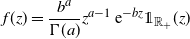 \begin{equation*}f(z) =\dfrac{b^{a}}{\Gamma(a) }z^{a-1}\,{\textrm{e}}^{-bz}\mathds{1}_{\mathbb{R}_{+}}(z)\end{equation*}
with respect to Lebesgue measure, where
 \begin{equation*}\Gamma(a) = \int_0^{\infty} s^{a-1}\exp({-}s)\,{\textrm{d}} s\quad \text{for all $a>0$}.\end{equation*}
The corresponding mean and variance are
 $a/b$
and
 $a/b^2$
respectively. Note also that if
 $Z_{1},\ldots,Z_{n}$
are independent gamma-distributed random variables with respective distributions
 $\Gamma_{0}( a_{1},b),\ldots,\Gamma_{0}( a_{n},b) ,$
where
 $a_1>0, \ldots, a_n>0, b>0$
, then
 $bZ_1$
and
 $\sum_{i=1}^{n}Z_{i}$
are gamma-distributed with parameters
 $(a_1,1)$
and
 $(\!\sum_{i=1}^{n}a_{i},b)$
, respectively. Finally, we recall some classic results for gamma distributions.
Lemma 3. ([Reference Müller and Stoyan16, page 62].) Let
 $Z_{1}$
and
 $Z_{2}$
be gamma-distributed random variables with parameters
 $( a_{1},b_{1}) $
and
 $( a_{2},b_{2}) $
, respectively, where
 $a_{i},b_{i}>0$
for
 $i=1,2$
. Then:
-
(a) If
$a_{1}\leq a_{2}$
and
$b_{1}\geq b_{2}$
, then
$Z_{1}\prec_{\textrm{lr}}Z_{2}$
, and hence
$Z_{1}\prec_{\textrm{hr}}Z_{2}$
and
$Z_{1}\prec_{\textrm{rh}}Z_{2}$
. -
(b) If
$a_{1}\geq a_{2}$
and
$a_{1}/b_{1}\leq a_{2}/b_{2}$
, then
$Z_{1}\prec_{\textrm{icx}}Z_{2}$
. -
(c) If
$b_{1}\leq b_{2}$
and
$a_{1}/b_{1}\leq a_{2}/b_{2}$
(and hence
$a_{1}\leq a_{2}$
), then
$Z_{1}\prec_{\textrm{icv}}Z_{2}$
.


Lemma 4. ([Reference Yu26].) Let
 $Z_i\sim\Gamma_0(a_i,b_i)$
,
 $i=1,\ldots,n$
, be independent gamma-distributed random variables. Let us set
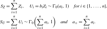 \begin{align*} S_{Z} & =\sum_{i=1}^{n}Z_{i},\quad U_{i}=b_{i}Z_{i}\sim\Gamma_{0}(a_{i},1) \quad\textit{for $i\in\{ 1,\ldots,n\} $,} \\* S_{U} & =\sum_{i=1}^{n}U_{i}\sim\Gamma_{0}\biggl( \sum_{i=1}^{n}a_{i},1\biggr) \quad\textit{and}\quad a_+=\sum_{i=1}^na_i. \end{align*}
Then:
-
(a)
$\beta^{-1}\,S_{U}\prec_{\textrm{hr}}S_{Z}$
is equivalent to
$\beta^{-1}\,S_{U}\prec_{\textrm{sto}}S_{Z}$
and it is true if and only if
\begin{equation*} \beta\geq\prod_{i=1}^{n}b_{i}^{{{a_{i}}/{a_{+}}}}.\end{equation*}
-
(b)
$\beta^{-1}\,S_{U}\prec_{\textrm{lr}}S_{Z}$
is equivalent to
$\beta^{-1}\,S_{U}\prec_{\textrm{rh}}S_{Z}$
and it is true if and only if
\begin{equation*} \beta\geq\dfrac{1}{a_{+}}\sum_{i=1}^{n}a_{i}b_{i}. \end{equation*}




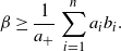
Lemma 5. ([Reference Marshall and Olkin15, Proposition 9.A.3].) Let
 $Z\sim\Gamma_{0}(a,b_{0})$
. Then Z is IFR if
 $a\geq1$
, DFR if
 $a\leq1$
, and DRHR for all
 $a>0$
.
3. Standard gamma processes
Here we recall the definitions as well as some properties of SGPs. Throughout the paper, we let
 $A\colon \mathbb{R}_{+}\rightarrow\mathbb{R}_{+}$
denote an increasing and continuous function with
 $A(0)=0$
and let
 $a({\cdot})$
denote its derivative (which exists almost surely).
3.1. Definition
Let
 $b_{0}$
be a positive constant. Recall that a standard (non-homogeneous) gamma process
 $\textbf{\textit{Y}}=(Y_{t})_{t \geq 0} \sim \Gamma _{0}(A(\!\cdot\!),b_0)$
, with
 $A(\!\cdot\!)$
as shape function and
 $b_0$
as scale parameter, is a stochastic process with independent, non-negative, and gamma-distributed increments:
 \begin{equation*}Y_{t}-Y_{s}\sim\Gamma_{0}{ (A(t)-A(s),b_{0})}\quad\text{for all $0<s<t$,}\end{equation*}
and such that
 $Y_{0}=0$
a.s. The PDF of an increment
 $Y_{t}-Y_{s}$
is then given by
 \begin{equation*} f(x)= \dfrac{b_0^{A(t)-A(s)}}{\Gamma (A(t)-A(s))} x^{A(t)-A(s)-1} \exp ({-b_0 x})\quad\text{for all $ x \geq 0$.}\end{equation*}
The mean and variance of
 $Y_t$
are given by
 $\mathbb{E}[Y_t]={A(t)}/{b_0}$
and
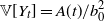 $ \mathbb{V}[Y_t]={A(t)}/{b_0^2}$
for all
 $t \geq 0$
, respectively. Hence the variance-to-mean ratio
 ${\mathbb{V}[Y_t]}/{\mathbb{E}[Y_t]} = b_0$
is constant over time.
3.2. Stochastic ordering and ageing properties for SGPs
We first review ageing properties and stochastic comparisons for the increments of a given SGP, and next provide stochastic comparisons between two SGPs with different parameters.
Based on Section 2.3 (and particularly Lemmas 3 and 5), the three following lemmas are easily obtained.
Lemma 6. Let
 $\textbf{\textit{Y}}=(Y_{t})_{t \geq 0}$
be an SGP with shape function
 $A(\!\cdot\!)$
and scale parameter
 $b_0$
. Then:
-
(a) If
$A( t+h)-A(t) \geq1$
,
$Y_{t+h}-Y_t$
is IFR; in particular,
$Y_{t}$
is IFR as soon as
$A( t) \geq1$
. -
(b) If
$A( t+h)-A(t) \leq1$
,
$Y_{t+h}-Y_t$
is DFR; in particular,
$Y_{t}$
is DFR as soon as
$A( t) \leq1$
. -
(c)
$Y_{t+h}-Y_t$
and
$Y_{t}$
are DRHR for all t and all h.






Lemma 7. Let
 $\textbf{\textit{Y}}=(Y_{t})_{t \geq 0}$
be an SGP with shape function
 $A(\!\cdot\!)$
and scale parameter
 $b_0$
. Then:
-
(a) If
$ 0\leq s\leq t$
, then
$Y_{s}\prec_{\textrm{lr}}Y_{t}$
. -
(b) If
$A(\!\cdot\!) $
is convex, then
$Y_{s+h}-Y_{s}\prec_{\textrm{lr}}Y_{t+h}-Y_{t}$
for all
$ 0\leq s\leq t$
and
$h\geq0$
. -
(c) If
$A(\!\cdot\!) $
is concave, then
$Y_{s+h}-Y_{s}\succ_{\textrm{lr}}Y_{t+h}-Y_{t}$
for all
$ 0\leq s\leq t$
and
$h\geq0$
.








Lemma 8. Let
 $\textbf{\textit{Y}}^{(i)}= \big( Y_{t}^{( i) }\big) _{t\geq0}\sim\Gamma_{0}(A_{i}(\!\cdot\!) ,b_{i})$
for
 $i\in\{ 1,2\} $
.
-
(a) If
$A_{1}(t) \leq A_{2}(t) $
and
$b_{1}\geq b_{2}$
, then
$Y_{t}^{( 1) }\prec_{\textrm{lr}}Y_{t}^{(2) }$
. -
(b) If
$A_{2}(\!\cdot\!) -A_{1}(\!\cdot\!) $
is an increasing function and
$b_{1}\geq b_{2}$
, then for all
$t,h\geq0$
,
$Y_{t+h}^{( 1) }-Y_{t}^{( 1) }\prec_{\textrm{lr}}Y_{t+h}^{( 2) }-Y_{t}^{( 2) }$
. -
(c) If
$A_{1}(t) \geq A_{2}(t) $
and
${{A_{1}(t)}/{b_{1}}} \leq {{A_{2}(t)}/{b_{2}}}$
, then
$Y_{t}^{( 1) }\prec_{\textrm{icx}}Y_{t}^{( 2) }$
. -
(d) If
$A_{2}(\!\cdot\!) -A_{1}(\!\cdot\!) $
is a decreasing function and
${{A_{2}(\!\cdot\!)}/{b_{2}}}-{{A_{1}(\!\cdot\!)}/{b_{1}}}$
is an increasing function, then
$Y_{t+h}^{( 1)}-Y_{t}^{( 1) }\prec_{\textrm{icx}}Y_{t+h}^{( 2) }-Y_{t}^{( 2) }$
for all
$t,h\geq0$
. -
(e) If
$A_{1}(t) \leq A_{2}(t) $
,
${{A_{1}(t)}/{b_{1}}} \leq {{A_{2}(t)}/{b_{2}}}$
and
$b_1\leq b_2$
, then
$Y_{t}^{( 1) }\prec_{\textrm{icv}}Y_{t}^{( 2) }$
. -
(f) If
$b_{1}\leq b_{2}$
and
${{A_{2}(\!\cdot\!)}/{b_{2}}}-{{A_{1}(\!\cdot\!)}/{b_{1}}}$
is an increasing function (and necessarily
$A_{2}(\!\cdot\!) -A_{1}(\!\cdot\!) $
too), then
$Y_{t+h}^{( 1)}-Y_{t}^{( 1) }\prec_{\textrm{icv}}Y_{t+h}^{( 2) }-Y_{t}^{( 2) }$
for all
$t,h\geq0$
.


















Finally, we come to present the properties of the crossing time of a given threshold
 $\ell$
, which can stand for the failure time of a system modeled by an SGP, as mentioned in the Introduction. Note that in the context of an SGP which is a pure jump process, the level
 $\ell$
is almost surely crossed by a jump, so that the level
 $\ell$
is almost surely never hit. That is why we call it a crossing time, and not a hitting time, which is the common vocabulary for continuous processes such as Wiener processes. The same remark is valid for an EGP hereafter. Note also that a threshold crossing time can also represent the time for a required preventative maintenance action if
 $\ell$
stands for a preventative threshold (lower than the failure threshold). In that case, the maintenance action is triggered as soon as the deterioration level is beyond
 $\ell$
(at time
 $\sigma_{\ell}$
), the aim being to avoid failures that could have unsafe or costly consequences.
The results below can be found in [Reference Sangüesa, Bada and Cha18] and [Reference Kahle, Mercier and Paroissin12].
Lemma 9. Let
 $\textbf{\textit{Y}}=(Y_{t})_{t \geq 0}$
be an SGP with shape function
 $A(\!\cdot\!)$
and scale parameter
 $b_0$
, and let
 $\ell>0$
.
-
(a) If
$A(\!\cdot\!)$
is convex, then
$\sigma_{\ell}$
is IFR. -
(b) If
$A(\!\cdot\!)$
is concave, then
$\sigma_{\ell}$
is DRHR.


4. Extended gamma processes
The aim of this section is to study how the results of Section 3 on SGPs can be adapted to EGPs. We first recall basic definitions and properties of EGPs in Section 4.1. Ageing properties and comparison results of EGP increments are next discussed in Sections 4.2 and 4.3. The comparison between two different EGPs is investigated in Section 4.4. Finally, ageing properties of threshold crossing times are studied in the context of EGPs in Section 4.5.
Henceforth we refer to an SGP by
 $\textbf{\textit{Y}}=(Y_{t})_{t \geq 0}$
and to an EGP by
 $\textbf{\textit{X}}=(X_{t})_{t \geq 0}$
.
4.1. Definition
Let
 $b\colon \mathbb{R}_{+}^*\rightarrow \mathbb{R}_{+}^*$
be a measurable positive function such that
 \begin{equation*} \int_{(0,t]}\dfrac{a(s)}{b(s)}\,{\textrm{d}} s<\infty \quad \text{for all $t > 0$.}\end{equation*}
Following [Reference Çinlar4] and [Reference Dykstra and Laud9], the process
 $\textbf{\textit{X}}=(X_{t})_{t\geq0}$
is said to be an EGP with shape function
 $A(\!\cdot\!)$
and scale function
 $b(\!\cdot\!)$
if
 $X_{t}$
can be represented as a stochastic integral with respect to an SGP
 $\textbf{\textit{Y}}$
with
 $Y_{t}\sim\Gamma_{0}(A(t),1)$
:
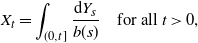 \begin{equation*} X_{t}=\int_{(0,t]}\dfrac{{\textrm{d}} Y_{s}}{b(s)} \quad \text{for all $t >0$,}\end{equation*}
and
 $X_{0}=0$
. If
 $b(\!\cdot\!)$
is constant and equal to
 $b_{0}$
, the EGP simply reduces to an SGP
 $\Gamma_{0}(A(t),b_0)$
. An EGP is much more flexible than an SGP and can be proved to have independent increments, and its distribution to be infinitely divisible. It allows us to model many possible behaviors for the system deterioration (see [Reference Al Masry, Mercier and Verdier1] for more precision). Also, an explicit formula is available for the Laplace transform of an increment [Reference Çinlar4], with
 \begin{equation*} \mathcal{L}_{X_{t+h}-X_{t}}(\lambda)\,:\!=\mathbb{E}\big( {\textrm{e}}^{-\lambda(X_{t+h}-X_{t})}\big) =\exp\biggl( -\int_{t}^{t+h}\log\biggl(1+\dfrac{\lambda}{b(s)}\biggr) a(s)\,{\textrm{d}} s\biggr)\end{equation*}
for all
 $t,\lambda\geq0$
and
 $h>0$
.
Finally, the mean and variance of an EGP are given by
 \begin{equation*} \mathbb{E}(X_{t})=\int_{(0,t]}\dfrac{a(s)}{b(s)}\,{\textrm{d}} s\quad \text{and}\quad \mathbb{V}(X_{t})=\int_{(0,t]}\dfrac{a(s)}{b(s)^{2}}\,{\textrm{d}} s \quad\text{for all $t>0$.}\end{equation*}
4.2. Ageing properties of EGP’s increments
We first explore the ageing properties of an EGP increment, as provided by Lemma 6 in the case of an SGP. We start with the DRHR property. With that aim, we begin with a technical lemma.
Lemma 10. Let
 $Z_i\sim \Gamma_0(a_i,b_i)$
,
 $i=1,\ldots,n$
, be n independent gamma-distributed random variables. Then
 $\sum_{i=1}^nZ_i$
is DRHR.
Proof. It is a direct consequence of the closure property of DRHR random variables under convolution [Reference Shaked and Shanthikumar21, Corollary 1.B.63], and of the fact that gamma random variables are DRHR (see Lemma 6). □
Next proposition shows that the DRHR property of an SGP increment remains valid for an EGP.
Proposition 1. Let
 $\textbf{\textit{X}}=(X_{t})_{t\geq0}\sim\Gamma(A(\!\cdot\!),b(\!\cdot\!))$
be an EGP. Then
 $X_{t}$
and
 $X_{t+h}-X_{t}$
are DRHR for all
 $h\geq0$
and all
 $t\geq0$
.
Proof. Note that it is enough to show that
 $X_{t+h}-X_{t}$
is DRHR. The proof is divided into two parts. Following some arguments developed in [Reference Al Masry, Mercier and Verdier1], we first assume that the scale function b (or the rate function
 $1/b$
) is a piecewise constant function given by
 \begin{equation}\dfrac{1}{b( v)} =\sum_{i=0}^{m}\dfrac{1}{b_{i}}\,\mathds{1}_{(u_{i},u_{i+1}]}( v) \quad \text{for all }v \geq 0,\end{equation}
where
 $u_{0}=0<u_{i}<u_{i+1}<u_{m+1}\leq+\infty$
for all
 $1\leq i\leq m-1$
and
 $b_{i}>0$
for all
 $1\leq i\leq m$
. Assuming
 $u_{i_{t}}<t \leq u_{i_{t}+1}$
,
 $u_{i_{t+h}}<t+h \leq u_{i_{t+h}+1}$
, and without loss of generality that
 $u_{i_{t}+1}<u_{i_{t+h}}$
, we have
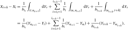 \begin{align*} X_{t+h}-X_{t} & =\dfrac{1}{b_{i_{t}}}\int_{(t,u_{i_{t}+1}]}\,{\textrm{d}} Y_{v}+\sum_{i=i_{t}+1}^{i_{t+h}-1}\dfrac{1}{b_{i}}\,\int_{(u_{i},u_{i+1}]}\,{\textrm{d}} Y_{v}+\dfrac{1}{b_{i_{t+h}}}\int_{(u_{i_{t+h}},t+h]}\,{\textrm{d}} Y_{v}\notag\\[3pt]
& =\dfrac{1}{b_{i_{t}}}( Y_{u_{i_{t}+1}}-Y_{t})+\sum_{i=i_{t}+1}^{i_{t+h}-1}\dfrac{1}{b_{i}}( Y_{u_{i+1}}-Y_{u_{i}})+\dfrac{1}{b_{i_{t+h}}}( Y_{t+h}-Y_{u_{i_{t+h}}}) ,\end{align*}
where
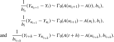 \begin{align*}\dfrac{1}{b_{i_t}}(Y_{u_{i_{t}+1}}-Y_{t}) &\sim\Gamma_{0}(A(u_{i_{t}+1}) -A(t),b_{i_{t}}),\\[3pt]\dfrac{1}{b_{i}}( Y_{u_{i+1}}-Y_{u_{i}}) &\sim\Gamma_{0}(A( u_{i+1}) -A( u_{i}),b_{i}),\\[3pt] \text{and}\quad \dfrac{1}{b_{i_{t+h}}}( Y_{t+h}-Y_{u_{i_{t+h}}}) &\sim\Gamma_{0}( A( t+h) -A( u_{i_{t+h}}),b_{i_{t+h}}).\end{align*}
The increment
 $X_{t+h}-X_{t}$
can therefore be written as a convolution of independent gamma random variables. This shows, by Lemma 10, that
 $X_{t+h}-X_{t}$
is DRHR when
 $b(\!\cdot\!) $
is piecewise constant.
We now consider a general function
 $b\colon \mathbb{R}_{+}^{\ast}\rightarrow\mathbb{R}_{+}^{\ast}$
. Then there exists an increasing sequence
 $( \beta^{( n) }(\!\cdot\!) ) _{n\in\mathbb{N}}$
of piecewise constant functions of the shape (2) that converges to
 ${{1}/{b}}$
. Let
 $( X_{t}^{( n) }) _{t\geq0}\sim\Gamma(A(\!\cdot\!),b^{( n) }(\!\cdot\!))$
with
 $b^{( n) }(t)={{1}/{(\beta^{( n) }}(t))}$
. We have
 \begin{equation*}\lim_{n\rightarrow+\infty}\mathcal{L}_{X_{t+h}^{( n) }-X_{t}^{( n) }}(\lambda) =\mathcal{L}_{X_{t+h}-X_t}( \lambda) \quad \text{for all $\lambda>0$}\end{equation*}
by the monotone convergence theorem, so that
 \begin{equation*}X_{t+h}^{(n)}-X_{t}^{( n) }\overset{\mathcal{D}}{\rightarrow}X_{t+h}-X_t\quad \text{when $n\rightarrow+\infty$}\end{equation*}
for all
 $t>0$
, where the symbol
 $\overset{\mathcal{D}}{\rightarrow}$
stands for convergence in distribution. The result is then easily derived from the piecewise constant case and letting
 $n\rightarrow+\infty$
(as the DRHR property is preserved by convergence in distribution; see [Reference Shaked and Shanthikumar21]). □
We now come to the DFR property of an EGP increment, in the case where
 $A(t+h)-A(t)$
is smaller than 1. Here again we begin with a technical lemma.
Lemma 11. Let
 $Z_i\sim \Gamma_0(a_i,b_i)$
,
 $i=1,\ldots,n$
, be n independent gamma-distributed random variables such that
 $\sum_{i=1}^{n}a_{i}\leq1$
(so that
 $a_{i}\leq1$
for all
 $i\in\{ 1,\ldots,n\} $
). Then
 $\sum_{i=1}^{n}Z_{i}$
is DFR.
Proof. The DFR property is known not to be stable through convolution in general, so the proof of Lemma 10 for the DRHR case should be adapted. Let us set
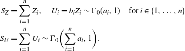 \begin{align*}S_{Z} & =\sum_{i=1}^{n}Z_{i},\quad U_{i}=b_{i}Z_{i}\sim\Gamma_{0}(a_{i},1) \quad\text{for $i\in\{ 1,\ldots,n\} $}\\*S_{U} & =\sum_{i=1}^{n}U_{i}\sim\Gamma_{0}\biggl( \sum_{i=1}^{n}a_{i},1\biggr) .\end{align*}
Using an argument similar to that in the proof of Theorem 3 of [Reference Yu26], we may write
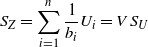 \begin{equation*}S_{Z}=\sum_{i=1}^{n}\dfrac{1}{b_{i}}U_{i}=V\,S_{U}\end{equation*}
with
 \begin{equation*}V=\sum_{i=1}^{n}\dfrac{1}{b_{i}}\dfrac{U_{i}}{S_{U}}.\end{equation*}
The random vector
 $( {{U_{1}}/{S_{U}}},\ldots,{{U_{n}}/{S_{U}}}) $
is known to be independent on
 $S_{U}$
, so V is also independent on
 $S_{U}$
. Then
 \begin{equation*}f_{S_{Z}}( z) =\int_{\mathbb{R}_{+}}f_{VS_{U}|V=v}( z)f_{V}( v) \,{\textrm{d}} v\end{equation*}
with
 $f_{VS_{U}|V=v}$
the conditional PDF of
 $VS_{U}$
given that
 $V=v$
. The distribution of
 $S_{Z}$
therefore appears as a mixture of the
 $vS_{U}$
. As
 $\sum_{i=1}^{n}a_{i}\leq1$
, we know that
 $S_{U}$
is DFR and
 $vS_{U}$
as well. Then the distribution of
 $S_{Z}$
appears as a mixture of DFR distributions, and since the DFR property is closed under mixture [Reference Marshall and Olkin15], the proof is completed. □
Proposition 2. Let
 $\textbf{\textit{X}}=(X_{t})_{t\geq0}\sim\Gamma(A(\!\cdot\!),b(\!\cdot\!))$
be an EGP. Let
 $h\geq0$
and
 $t\geq0$
be such that
 $A(t+h)-A(t)\leq1$
. Then
 $X_{t+h}-X_{t}$
is DFR. In particular,
 $X_{t}$
is DFR as soon as
 $A(t)\leq1$
.
Proof. We can use similar arguments as for the proof of Proposition 1 as the DFR property is also preserved by convergence in distribution; see [Reference Shaked and Shanthikumar21]. □
We now explore the possibly IFR property in the case where
 $A(t+h)-A(t)$
is larger than 1, and for that, a numerical example is considered.
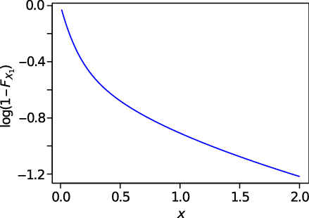
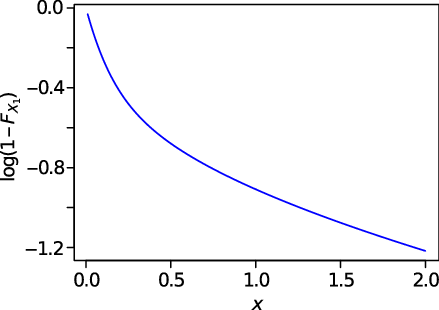
Example 1. Let us consider
 $A( t)=t$
(which is both a concave and convex function) and let
 \begin{equation*} b( t) =10\,\mathds{1}_{[0,0.75)}( t) +0.1\,\mathds{1}_{[0.75,\infty)}( t) \end{equation*}
(decreasing function). The function
 $\log(\bar{F}_{X_{1}})$
is plotted in Figure 1 for
 $t=1$
(and hence
 $A(t)=1$
). As can be seen,
 $\log(\bar{F}_{X_{1}})$
is not a concave function, which shows that
 $X_{1}$
is not IFR.
Considering the increasing function
 \begin{equation*} b( t) =0.1\,\mathds{1}_{[0,0.25)}( t) +10\,\mathds{1}_{[0.25,\infty)}( t) \end{equation*}
provides the same distribution for
 $X_{1}$
(convolution of the gamma distributions
 $\Gamma_{0}( 0.25,0.1) $
and
 $\Gamma_{0}( 0.75,10) $
) and the same conclusion.
Based on the above example, we can see that even considering a convex or a concave shape function and a monotone scale function, an increment
 $X_{t+h}-X_t$
need not be IFR when the shape parameter
 $A(t+h)-A(t)$
is larger than 1. Hence it seems difficult to find sufficient conditions to ensure the IFR property of an increment. As a by-product, we observe that not all ageing properties provided in Lemma 6 for SGPs remain true for an EGP.
4.3. Monotonicity of an EGP and stochastic comparison between increments
Here we explore how to adapt the results of Lemma 7 in the case of an EGP. We first look at the possible monotonicity of an EGP with respect to the likelihood ratio order. For that, a numerical example is considered.
Example 2. Let us consider
 $A( t) =t$
and
 $b( t) =0.1\,\mathds{1}_{[0,0.25)}( t) +10\,\mathds{1}_{[0.25,\infty)}( t)$
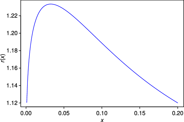
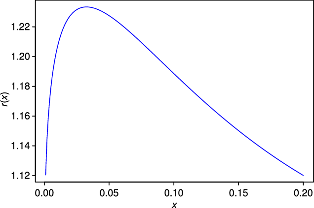
. The function
 $r( x) ={\bar{F}_{X_{1}}( x) }/{ \bar{F}_{X_{0.25}}( x) }$
is plotted in Figure 2. We can observe that the function r(x) is not monotone with respect to x. Based on Definition 1, we can derive that
 $X_{0.25}$
and
 $X_{1}$
are not comparable with respect to the hazard rate order. Hence they are not comparable with respect to the likelihood ratio order either.
Plot of
 $\log(\bar{F}_{X_{1}}(t)) $
with respect to t for
 $A( t)=t$
and
 $b( t) =10\,\mathds{1}_{[0,0.75)}( t) +0.1\,\mathds{1}_{[0.75,\infty)}( t) $
.
Plot of
 $r( x) ={\bar{F}_{X_{1}}( x) }/{ \bar{F}_{X_{0.25}}( x) }$
as a function of x for
 $A( t) =t$
and
 $b( t) =0.1\,\mathds{1}_{[0,0.25)}( t) +10\,\mathds{1}_{[0.25,\infty)}( t)$
.
Remark 2. Based on the above example, we can see that the relationship
 $X_{s}\prec_{\textrm{lr}}X_{t}$
for
 $s < t$
is not valid in a general setting. To be more specific, considering a convex or a concave shape function and an increasing scale function, the property need not be true. However, we could not find any numerical counterexample with
 $A(t)=t$
(both convex and concave) and a decreasing scale function, and the property might hence be true under such assumptions. Unfortunately we have not been able to prove it, so the question remains open. Note that the proof would require likelihood-ratio comparison results for convolution of heterogeneous gamma distributions with shape parameter smaller than 1 (tending to 0, in a similar spirit as for the proof of Proposition 1). This seems quite difficult as it seems that all the results from the literature are valid for shape parameters larger than 1 (see e.g. [Reference Zhao27]). Hence it is quite a challenging (open) question.
Even though, under specific conditions, we were not able to conclude the possible likelihood-ratio monotonicity of an EGP, we now show its monotonicity with respect to the reversed hazard rate order under any conditions.
Proposition 3. Let
 $\textbf{\textit{X}}=(X_{t})_{t\geq0}\sim\Gamma(A(t),b(t))$
be an EGP. Then, for all
 $s<t$
, we have
 \begin{equation*}X_{s}\prec_{\textrm{rh}}X_{t}.\end{equation*}
Proof. Let
 $s<t$
. As
 $X_{t}-X_{s}\geq 0$
, it is easy to check that
 \begin{equation*}0\prec_{\textrm{rh}}X_{t}-X_{s}.\end{equation*}
Since
 $X_s$
is DRHR (see Proposition 1), we derive from [Reference Shaked and Shanthikumar21, Lemma 1.B.44] that
 $X_{s}=0+X_{s}\prec_{\textrm{rh}}X_{t}=( X_{t}-X_{s}) +X_{s}$
, which achieves the proof. □
We now provide comparison results between increments in the reversed hazard rate ordering. We begin with a technical lemma.
Lemma 12. Let
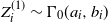 $Z_i^{(1)}\sim \Gamma_0(a_i,b_i)$
and
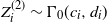 $Z_i^{(2)}\sim \Gamma_0(c_i,d_i)$
,
 $i=1,\ldots,n$
, such that
 $a_i\leq c_i$
and
 $b_i\geq d_i$
for all i. Then
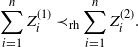 \begin{equation*}\sum_{i=1}^{n}Z_i^{(1)}\prec_{\textrm{rh}}\sum_{i=1}^{n}Z_i^{(2)}.\end{equation*}
Proof. From Lemma 3 we have
 \begin{equation*}Z_i^{(1)}\prec_{\textrm{lr}}Z_i^{(2)}\quad\text{for all $i=1,\ldots,n$,}\end{equation*}
so that
 \begin{equation*}Z_i^{(1)}\prec_{\textrm{rh}}Z_i^{(2)}\quad \text{for all $i=1,\ldots,n$.}\end{equation*}
As the reversed hazard rate order is stable under the convolution of DRHR random variables [Reference Shaked and Shanthikumar21, Theorem 1.B.45], the result follows. □
Proposition 4. Let
 $\textbf{\textit{X}}=(X_{t})_{t\geq0}\sim\Gamma(A(t),b(t))$
be an EGP. Assume that
-
•
$A(\!\cdot\!) $
is convex, -
•
$b(\!\cdot\!) $
is decreasing.


Then, for all
 $s\leq t$
and all
 $h>0$
,
 \begin{equation*}X_{s+h}-X_{s}\prec_{\textrm{rh}}X_{t+h}-X_{t}.\end{equation*}
Proof. Let
 $s\leq t\leq t+h$
. Here again we first consider the case where
 $b(\!\cdot\!) $
is piecewise constant (and decreasing). Then (0, h] is the union of a finite number of disjoint intervals
 $(u_{i},u_{i+1}]$
,
 $0\leq i\leq n$
such that
 $b( s+z) $
is constant for all
 $z\in(u_{i},u_{i+1}]$
and all
 $0\leq i\leq n$
. Cutting each of these intervals into pieces when necessary, we can construct disjoint intervals
 $(v_{j},v_{j+1}]$
for
 $0\leq j\leq m$
with
 $v_{0}=0$
and
 $v_{m+1}=h$
, such that
 $\bigcup_{j=0}^{m}(v_{j},v_{j+1}]=(0,h]$
and on which both
 $b( s+z) $
and
 $b( t+z) $
are constant for all
 $z\in(v_{j},v_{j+1}]$
and all
 $0\leq j\leq m$
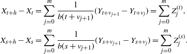
. This provides
 \begin{align*}X_{t+h}-X_{t} & =\sum_{j=0}^{m}\dfrac{1}{b( t+v_{j+1}) }(Y_{t+v_{j+1}}-Y_{t+v_{j}})=\sum_{j=0}^mZ_j^{(t)} ,\\*X_{s+h}-X_{s} & =\sum_{j=0}^{m}\dfrac{1}{b( s+v_{j+1}) }(Y_{s+v_{j+1}}-Y_{s+v_{j}})=\sum_{j=0}^mZ_j^{(s)} .\end{align*}
For all
 $j=1,\ldots,m$
, we have
 \begin{equation*}Z_j^{(z)}\sim\Gamma_{0}( A(z+v_{j+1}) -A( z+v_{j}) ,b(z+v_{j+1})) \quad\text{for $z\in\{s,t\} $}\end{equation*}
with
 \begin{equation*}A( s+v_{j+1}) -A( s+v_{j}) \leq A(t+v_{j+1}) -A( t+v_{j})\end{equation*}
and
 \begin{equation*}b(s+v_{j+1})\geq b(t+v_{j+1})\end{equation*}
because A is convex and b is decreasing. From Lemma 12 we then obtain
 \begin{equation*}X_{s+h}-X_{s}\prec_{\textrm{rh}}X_{t+h}-X_{t}.\end{equation*}
For a general decreasing function b, we proceed as in the proof of Proposition 1, and the result follows since
 $\prec_{\textrm{rh}}$
is preserved by convergence in distribution.□
Reversing the assumptions, we obtain a reversed inequality, as provided in the following proposition. The proof is similar and is omitted.
Proposition 5. Let
 $\textbf{\textit{X}}=(X_{t})_{t\geq0}\sim\Gamma(A(t),b(t))$
be an EGP. Assume that
-
•
$A(\!\cdot\!) $
is concave, -
•
$b(\!\cdot\!) $
is increasing.


Then, for all
 $s\leq t$
and all
 $h>0$
,
 \begin{equation*}X_{s+h}-X_{s}\succ_{\textrm{rh}}X_{t+h}-X_{t}.\end{equation*}
Remark 3. In Propositions 4 and 5, the monotonicity of
 $b(\!\cdot\!)$
is essential. Indeed, it is not difficult to provide a counterexample to the previous results when the monotonicity assumption is no longer satisfied. Let
 $A(t)=t$
and
 $b(t)=1/2\,\mathds{1}_{[0,1)}(t)+1/3\,\mathds{1}_{[1,2)}(t)+1\,\mathds{1}_{[2,3)}(t) +1/4\,\mathds{1}_{[3,\infty)}(t)$
(which is not monotonic). Then
 \begin{equation*}X_2-X_0\overset{\mathcal{D}}{=}2Y_1+3Y_2\,\,\textrm{and}\,\,X_4-X_2\overset{\mathcal{D}}{=}Y_3+4Y_4,\end{equation*}
where
 $\overset{\mathcal{D}}{=}$
means ‘is identically distributed as’ and where
 $Y_i\sim\Gamma(1,1)$
for
 $i=1,\ldots,4$
. As noted by Diaconis and Perlman [Reference Diaconis and Perlman6], we have
 $V[X_2-X_0]<V[X_4-X_2]$
, so the distributions of the two increments are not identical. However, they share the same expectation (
 $E[X_2-X_0]=E[X_4-X_2]$
), which entails that the sign of
 $F_{X_2-X_0}(x)-F_{X_4-X_2}(x)$
changes at least once on
 $(0,\infty)$
(in fact exactly once; see [Reference Diaconis and Perlman6, Proposition 2.1]). As a consequence, the two increments are not comparable with respect to the usual stochastic order, and hence they are not comparable with respect to the hr, rh, and lr orders either.
4.4. Stochastic comparisons between two EGPs
Here we provide comparison results between two different EGPs.
Proposition 6. Let
 \begin{equation*} \textbf{\textit{X}}^{(i)}=\big( X_{t}^{( i) }\big) _{t\geq0}\sim\Gamma (A_{i}(\!\cdot\!) ,b_{i}(\!\cdot\!))\quad\textit{for $i\in\{ 1,2\}$.} \end{equation*}
Assume that
-
•
$A_{2}(\!\cdot\!)-A_{1}(\!\cdot\!)$
is increasing, -
•
$b_1(t)\geq b_2(t)$
for all
$t\geq0$
.


Then, for all
 $t\geq0$
and all
 $h\geq0$
,
 \begin{equation*}X_{t+h}^{(1)}-X_t^{(1)}\prec_{\textrm{rh}}X_{t+h}^{(2)}-X_t^{(2)}.\end{equation*}
As a specific case, for all
 $t\geq0$
,
 \begin{equation*}X_t^{(1)}\prec_{\textrm{rh}}X_t^{(2)}.\end{equation*}
Proof. Let
 $t\geq0$
and
 $h\geq0$
. Here again we first consider the case where the functions
 $b_1(\!\cdot\!)$
and
 $b_2(\!\cdot\!)$
are piecewise constant, and we proceed as in the proof of Proposition 4. It is then possible to consider disjoint intervals
 $(v_{j},v_{j+1}]$
for
 $0\leq j\leq m$
with
 $v_{0}=0$
and
 $v_{m+1}=h$
, such that
 $\bigcup_{j=0}^{m}(v_{j},v_{j+1}]=(0,h]$
and on which both
 $b_1(t+z) $
and
 $b_2( t+z) $
are constant for all
 $z\in(v_{j},v_{j+1}]$
and all
 $0\leq j\leq m$
. This provides
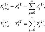 \begin{align*}X_{t+h}^{(1)}-X_{t}^{(1)} & =\sum_{j=0}^mZ_j^{(1)} ,\\*X_{t+h}^{(2)}-X_{t}^{(2)} & =\sum_{j=0}^mZ_j^{(2)},\end{align*}
with
 \begin{equation*}Z_j^{(i)}\sim\Gamma_{0}( A_i(t+v_{j+1}) -A_i( t+v_{j}) ,b_i(t+v_{j+1})) \quad\text{for $i\in\{ 1,2\} $.}\end{equation*}
By hypothesis, for all
 $j=1,\ldots,m$
,
 \begin{equation*}A_2(t+v_{j+1})-A_1(t+v_{j+1})\geq A_2( t+v_{j})-A_1( t+v_{j}),\end{equation*}
since
 $v_{j+1}\geq v_{j}$
, which leads to
 \begin{equation*}A_2(t+v_{j+1})-A_2( t+v_{j})\geq A_1(t+v_{j+1})-A_1( t+v_{j}).\end{equation*}
Moreover,
 \begin{equation*}b_1(t+v_{j+1})\geq b_2(t+v_{j+1}).\end{equation*}
From Lemma 12 we then obtain
 \begin{equation*}X_{t+h}^{(1)}-X_{t}^{(1)}\prec_{\textrm{rh}}X_{t+h}^{(2)}-X_{t}^{(2)},\end{equation*}
which achieves the proof in the case of piecewise constant scale functions.
For general functions
 $b_i$
,
 $i=1,2$
, we proceed as in the proof of Proposition 1, and the result follows since
 $\prec_{\textrm{rh}}$
is preserved by convergence in distribution. □
The above proposition allows us to compare an EGP and an SGP that share the same shape function, as stated in the following corollary. It is an immediate consequence and it is stated without proof.
Corollary 1. Let
 \begin{equation*} \textbf{\textit{Y}}=(Y_t)_{t\geq0}\sim\Gamma_0(A(t),\beta)\ \text{(SGP)},\quad \textbf{\textit{X}}=(X_t)_{t\geq0}\sim\Gamma(A(t),b(t))\ \text{(EGP).}\end{equation*}
We have the following results.
-
(a) If
$b(t)\leq \beta$
for all t in a given interval
$[t_1,t_2]$
, then
for all
\begin{equation*} Y_{t+h}-Y_{t}\prec_{\textrm{rh}}X_{t+h}-X_{t}, \end{equation*}
$t\in[t_1,t_2[$
and all h such that
$t+h\leq t_2$
.
-
(b) In particular, if
$b(t)\leq \beta$
for all
$t\geq0$
, then
\begin{equation*} Y_{t}\prec_{\textrm{rh}}X_t. \end{equation*}
-
(c) The inequalities of the two previous points are reversed if
$b(t)\geq \beta$
.





By considering more stringent constraints on parameter
 $\beta$
and function
 $b(\!\cdot\!)$
, it is possible to give necessary and sufficient conditions for the hr and lr orders.
Proposition 7. Let
 \begin{equation*} \textbf{\textit{Y}}=( Y_{t}) _{t\geq0}\sim\Gamma_{0}( A(\!\cdot\!) ,\beta) \ \textit{(SGP)},\quad \textbf{\textit{X}}=( X_{t}) _{t\geq0}\sim \Gamma( A(\!\cdot\!) ,b(\!\cdot\!) ) \ \textit{(EGP)}. \end{equation*}
Then:
-
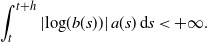
(a) Assume that there exists
$b_{0}>0$
such that
$b_{0}\leq b(s) $
for all
$s\in[ t,t+h] $
and
Then
\begin{equation*} \int_{t}^{t+h}\vert\textrm{log}( b( s) ) \vert \,a( s)\,{\textrm{d}} s<+\infty. \end{equation*}
$Y_{t+h}-Y_{t}\prec_{\textrm{hr}}X_{t+h}-X_{t}$
is equivalent to
$Y_{t+h}-Y_{t}\prec_{\textrm{sto}}X_{t+h}-X_{t}$
and it is true if and only if
(3)
\begin{equation}\log(\beta) \geq\dfrac{1}{A( t+h) -A( t) }\int_{t}^{t+h}\log( b( s) ) \,a( s) \,{\textrm{d}} s.\end{equation}
-
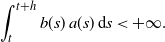
(b) Assume that
Then
\begin{equation*} \int_{t}^{t+h}b( s) \,a( s)\,{\textrm{d}} s<+\infty. \end{equation*}
$Y_{t+h}-Y_{t}\prec_{\textrm{lr}}X_{t+h}-X_{t}$
is equivalent to
$Y_{t+h}-Y_{t}\prec_{\textrm{rh}}X_{t+h}-X_{t}$
and it is true if and only if
(4)
\begin{equation}\beta\geq\dfrac{1}{A( t+h) -A( t) }\int_{t}^{t+h}b( s)\,a( s) \,{\textrm{d}} s.\end{equation}








Proof. Assume first that
 $b(\!\cdot\!) $
is piecewise constant with
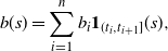 \begin{equation*} b( s) =\sum_{i=1}^{n}b_{i}\textbf{1}_{(t_{i},t_{i+1}]}(s) , \end{equation*}
where
 $t_{1}=t$
,
 $t_{n+1}=t+h$
and let
 $a_{i}=A(t_{i+1}) -A( t_{i}) $
for
 $i\in\{ 1,\ldots,n\} $
. Then, using the notation of Lemma 4,
 $X_{t+h}-X_{t}$
and
 $Y_{t+h}-Y_{t}$
are identically distributed as
 $S_{Z}$
and
 $\beta^{-1}\,S_{U}$
, respectively. In that case, we have
 \begin{equation*}\dfrac{1}{A( t+h) -A( t) }\int_{t}^{t+h}\log(b( s) ) \,a( s) \,{\textrm{d}} s=\dfrac{1}{a_{+}}\sum_{i=1}^{n}\int_{t_{i}}^{t_{i+1}}\log( b( s) )\,\,a( s) \,{\textrm{d}} s=\dfrac{1}{a_{+}}\sum_{i=1}^{n}a_{i}\log(b_{i})\end{equation*}
and, using Lemma 4, condition (3) is equivalent to
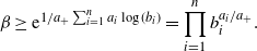 \begin{equation*}\beta\geq {\textrm{e}}^{{{1}/{a_{+}}}\sum_{i=1}^{n}a_{i}\log( b_{i})}=\prod_{i=1}^{n}b_{i}^{{{a_{i}}/{a_{+}}}}.\end{equation*}
This proves the first point in the case of a piecewise constant function
 $b(\!\cdot\!) $
.
Now let us consider the case of a general function
 $b(\!\cdot\!) $
and let
 $( b_{n}(\!\cdot\!) ) _{n\in\mathbb{N}}$
be an increasing sequence of piecewise constant positive functions on
 $\mathbb{R}_{+}^{\ast}$
, such that
 $b_{n}( s) $
tends to b(s) when
 $n\rightarrow+\infty$
for all
 $s\in\lbrack t,t+h]$
, and let
 $( X_{t}^{( n) }) _{t\geq0}\sim\Gamma(A(\!\cdot\!) ,b_{n}(\!\cdot\!) ) $
.
Assume that condition (3) is true. Then, as
 $b_{n}( s)\leq b( s) $
, condition (3) is also true when b(s) is replaced by
 $b_{n}( s) $
, and hence
 $Y_{t+h}-Y_{t}\prec_{\textrm{hr}}X_{t+h}^{( n) }-X_{t}^{( n)}$
and
 $Y_{t+h}-Y_{t}\prec_{\textrm{sto}}X_{t+h}^{( n) }-X_{t}^{(n) }$
. Letting n go to infinity, we get that
 $Y_{t+h}-Y_{t}\prec_{\textrm{hr}}X_{t+h}-X_{t}$
and
 $Y_{t+h}-Y_{t}\prec_{\textrm{sto}}X_{t+h}-X_{t}$
.
Conversely, assume that
 $Y_{t+h}-Y_{t}\prec_{\textrm{sto}}X_{t+h}-X_{t}$
(or
 $Y_{t+h}-Y_{t}\prec_{\textrm{hr}}X_{t+h}-X_{t}$
). Observe that as
 $( b_{n}(\!\cdot\!) ) _{n\in\mathbb{N}}$
increases with n,
 $X_{t+h}^{( n) }-X_{t}^{( n) }$
decreases in the rh ordering (due to Proposition 6), and hence also in the usual stochastic ordering, when n increases.
Then
 \begin{equation*}\bar{F}_{Y_{t+h}-Y_{t}}( x) \leq\bar{F}_{X_{t+h}-X_{t}}(x) =\lim_{m\rightarrow+\infty}\bar{F}_{X_{t+h}^{( m)}-X_{t}^{( m) }}( x) \leq\bar{F}_{X_{t+h}^{(n) }-X_{t}^{( n) }}( x)\end{equation*}
for all
 $x\in\mathbb{R}$
and all
 $n\in\mathbb{N}$
. This implies that
 $Y_{t+h}-Y_{t}\prec_{\textrm{sto}} X_{t+h}^{( n) }-X_{t}^{( n)}$
, and hence condition (3) is true for
 $b_{n}(\!\cdot\!) $
:
 \begin{equation} \log( \beta) \geq\dfrac{1}{A( t+h) -A( t)}\int_{t}^{t+h}\log( b_{n}( s) ) \,a( s)\,{\textrm{d}} s\quad\text{for all $n\in\mathbb{N}^{\ast}$.}\end{equation}
As
 $\vert \textrm{log}( b_{n}(s) ) \vert \leq\vert \textrm{log}( b_{0})\vert +\vert \textrm{log}( b( s) ) \vert $
, we get by dominated convergence
 \begin{equation*}\lim_{n\rightarrow+\infty}\int_{t}^{t+h}\log( b_{n}( s)) \,a( s) \,{\textrm{d}} s=\int_{t}^{t+h}\log( b( s)) \,a( s) \,{\textrm{d}} s.\end{equation*}
Then, letting n go to infinity in (5) tells us that condition (3) is true for
 $b(\!\cdot\!) $
, and the first point is true. The second point is similar and its proof is omitted. □
Note that when condition (3) is not fulfilled, then
 $Y_{t+h}-Y_{t}$
and
 $X_{t+h}-X_{t}$
are not comparable with respect to the hazard rate ordering, as can be easily checked via a counterexample. The same is true for condition (4).
Note also that, under the conditions of Proposition 6, the results obtained for the rh order are also valid for the usual stochastic order, and hence also for both increasing convex and concave orders. We now provide other conditions for the increasing convex and concave orders, which extend some results from Lemma 8 (points (d) and (f)) to EGPs.
Proposition 8. Let
 \begin{equation*} \textbf{\textit{X}}^{(i)}=\big( X_{t}^{( i) }\big) _{t\geq0}\sim\Gamma (A_{i}(\!\cdot\!) ,b_{i}(\!\cdot\!))\quad for\ \textit{$i\in\{ 1,2\} $.} \end{equation*}
Assume that
-
•
$A_{2}(\!\cdot\!)-A_{1}(\!\cdot\!)$
is decreasing, -
•
${{A_{2}(\!\cdot\!)}/{b_2(\!\cdot\!)}} - {{A_{1}(\!\cdot\!)}/{b_1(\!\cdot\!)}} $
is increasing, -
•
$b_{1}(\!\cdot\!)$
is decreasing and
$b_{2}(\!\cdot\!)$
is increasing.




Then, for all
 $t\geq0$
and all
 $h\geq0$
,
 \begin{equation*}X_{t+h}^{(1)}-X_t^{(1)}\prec_{\textrm{icx}}X_{t+h}^{(2)}-X_t^{(2)}.\end{equation*}
As a specific case, for all
 $t\geq0$
,
 \begin{equation*}X_t^{(1)}\prec_{\textrm{icx}}X_t^{(2)}.\end{equation*}
Proof. Let
 $t\geq0$
and
 $h\geq0$
. Following the proof of Proposition 6, we have
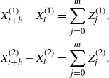 \begin{align*}X_{t+h}^{(1)}-X_{t}^{(1)} & =\sum_{j=0}^mZ_j^{(1)} ,\\*X_{t+h}^{(2)}-X_{t}^{(2)} & =\sum_{j=0}^mZ_j^{(2)},\end{align*}
with
 \begin{equation*}Z_j^{(z)}\sim\Gamma_{0}( A_z(t+v_{j+1}) -A_z( t+v_{j}) ,b_z(t+v_{j+1}))\quad\text{for $z\in\{1,2\} $.}\end{equation*}
By hypothesis, for all
 $j=1,\ldots,m$
,
 \begin{equation*}A_2(t+v_{j+1})-A_1(t+v_{j+1})\leq A_2( t+v_{j})-A_1( t+v_{j}),\end{equation*}
since
 $v_{j+1}\geq v_{j}$
, which leads to
 \begin{equation*}A_2(t+v_{j+1})-A_2( t+v_{j})\leq A_1(t+v_{j+1})-A_1( t+v_{j}).\end{equation*}
Moreover,
 \begin{equation*}\dfrac{A_{2}(t+v_{j+1})}{b_2(t+v_{j+1})} - \dfrac{A_{1}(t+v_{j+1})}{b_1(t+v_{j+1})} \geq \dfrac{A_{2}(t+v_{j})}{b_2(t+v_{j})} - \dfrac{A_{1}(t+v_{j})}{b_1(t+v_{j})} .\end{equation*}
This implies that
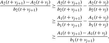 \begin{align*}\dfrac{A_{2}(t+v_{j+1})-A_{2}(t+v_{j})}{b_2(t+v_{j+1})} &\geq\dfrac{A_{2}(t+v_{j+1})}{b_2(t+v_{j+1})} - \dfrac{A_{2}(t+v_{j})}{b_2(t+v_{j})} \\[3pt]& \geq \dfrac{A_{1}(t+v_{j+1})}{b_1(t+v_{j+1})}- \dfrac{A_{1}(t+v_{j})}{b_1(t+v_{j})}\\[3pt]& \geq\dfrac{A_{1}(t+v_{j+1})-A_{1}(t+v_{j})}{b_1(t+v_{j+1})},\end{align*}
since
 $b_{1}(\!\cdot\!)$
is decreasing and
 $b_{2}(\!\cdot\!)$
is increasing.
From Lemma 8, we then have, for all
 $j=1,\ldots,m$
,
 \begin{equation*}Z_j^{(1)}\prec_{\textrm{icx}}Z_j^{(2)}.\end{equation*}
As the increasing convex order is stable under convolution [Reference Shaked and Shanthikumar21, Theorem 4.A.8], then
 \begin{equation*}X_{t+h}^{(1)}-X_{t}^{(1)}\prec_{\textrm{icx}}X_{t+h}^{(2)}-X_{t}^{(2)}.\end{equation*}
We now consider a general function
 $b\colon \mathbb{R}_{+}^{\ast}\rightarrow\mathbb{R}_{+}^{\ast}$
. Then there exist two increasing sequences
 $( \beta^{( i,n) }(\!\cdot\!) ) _{n\in\mathbb{N}}$
of piecewise constant functions of the shape (2) that converges to
 ${1}/{b_i}$
with
 $i\in\{ 1,2\} $
. Let
 $( X_{t}^{( i,n) })_{t\geq 0} \sim\Gamma(A_i(\!\cdot\!),b^{( i,n) }(\!\cdot\!))$
with
 $b^{( i,n) }(t)={1}/{\beta^{( i,n) }(t)}$
.
We have
 \begin{equation*}\lim_{n\rightarrow+\infty}\mathcal{L}_{X_{t+h}^{( i,n) }-X_{t}^{( i,n) }}(\lambda) ={ \mathcal{L}_{X_{t+h}^{(i)}-X_t^{(i)}}( \lambda)} \quad \text{for all $\lambda>0$}\end{equation*}
by the monotone convergence theorem, so
 \begin{equation*}X_{t+h}^{( i,n) }-X_{t}^{( i,n) }\overset{\mathcal{D}}{\rightarrow}X_{t+h}^{(i)}-X_t^{(i)}\quad\text{when $n\rightarrow+\infty$}\end{equation*}
for
 $i\in\{1,2\}$
.
Now we show that the previous convergence result also holds in the
 $L_1$
sense. First note that
 \begin{equation}\mathbb{E}\big[\big|\big({X_{t+h}^{(i,n)}}-X_{t}^{(i,n)}\big) -\big({X_{t+h}^{(i)}}-X_{t}^{(i)}\big)\big|\big] \leq \mathbb{E}\big[\big|{X_{t+h}^{(i,n)}}-{X_{t+h}^{(i)}}\big|\big] +\mathbb{E}\big[\big|X_{t}^{(i,n)} -X_{t}^{(i)}\big|\big]\end{equation}
with
 \begin{equation*}\mathbb{E}\big[\big|X_{t}^{( i,n)}-X_{t}^{(i)}\big|\big] \leq \mathbb{E}\biggl[\int_{(0,t]} \bigg| \beta^{( i,n)} (s)-\dfrac{1}{b_i (s)}\bigg|\,{\textrm{d}} Y(s)\biggr] \underset{n \rightarrow +\infty}\rightarrow 0\end{equation*}
by dominated convergence, because
 $| \beta^{( i,n)} (s)-{1}/{b_i (s)}|\leq 2 /{b_i (s)}$
and
 \begin{equation*}\mathbb{E}\biggl[\int_{(0,t]} \dfrac{1}{b_i(s)}\,{\textrm{d}} Y(s)\biggr] =\mathbb{E}\big(X_t^{(i)}\big)<+\infty.\end{equation*}
See Section 4.1.
The same reasoning shows that
 \begin{equation*}\mathbb{E}\big[\big|{X_{t+h}^{(i,n)}}-{X_{t+h}^{(i)}}\big|\big]\rightarrow 0,\end{equation*}
which allows us to conclude from (6) that
 \begin{equation*}X_{t+h}^{( i,n) }-X_{t}^{( i,n) }\overset{{L}^1}{\rightarrow}X_{t+h}^{(i)}-X_t^{(i)}\quad \text{when}\ n\rightarrow+\infty.\end{equation*}
Finally, the result is easily derived from [Reference Shaked and Shanthikumar21, Theorem 4.A.8] and from the piecewise constant case. □
Example 3. One can check that the assumptions of Proposition 8 are satisfied for
 $A_1(t)=\log(2t+1)$
,
 $A_2(t)=\log(t+1)$
,
 $b_1(t)={1}/(t+1)+2$
, and
 $b_2(t)=1-{1}/(t+2)$
. Note that this example does not fulfill the conditions of Proposition 6, and hence Proposition 8 provides new results when compared to Proposition 6.
We now provide similar results for the increasing concave order. The proof follows the same steps as in Proposition 8 and is omitted.
Proposition 9. Let
 $\textbf{\textit{X}}^{(i)}=\big( X_{t}^{( i) }\big) _{t\geq0}\sim\Gamma(A_{i}(\!\cdot\!) ,b_{i}(\!\cdot\!))$
for
 $i\in\{ 1,2\} $
. Assume that
-
•
${b_1(t )} \leq {b_2(t)} $
for all
$t\geq0$
, -
•
$b_{1}(\!\cdot\!)$
is decreasing and
$b_{2}(\!\cdot\!)$
is increasing, -
•
${{A_{2}(\!\cdot\!)}/{b_2(\!\cdot\!)}} - {{A_{1}(\!\cdot\!)}/{b_1(\!\cdot\!)}} $
is increasing (and hence
$A_{2}(\!\cdot\!)-A_{1}(\!\cdot\!)$
is also increasing).




Then, for all
 $t\geq0$
and all
 $h\geq0$
,
 \begin{equation*}X_{t+h}^{(1)}-X_t^{(1)}\prec_{\textrm{icv}}X_{t+h}^{(2)}-X_t^{(2)}.\end{equation*}
As a specific case, for all
 $t\geq0$
,
 \begin{equation*}X_t^{(1)}\prec_{\textrm{icv}}X_t^{(2)}.\end{equation*}
Example 4. One can check that the assumptions of Proposition 9 are satisfied for
 $A_1(t)=\log({{t}/{2}}+1)$
,
 $A_2(t)=\exp(t)-1$
,
 $b_1(t)={{1}/{(t+1)}}+{{1}/{2}}$
, and
 $b_2(t)=2-{{1}/{(t+2)}}$
. Here again this example does not fulfill the conditions of Proposition 6, and Proposition 9 provides new results when compared to Proposition 6.
4.5. Ageing properties of threshold crossing times
We finally come to ageing properties of threshold crossing times. We begin with a first result when the threshold is an IFR random variable.
Proposition 10. Let L be an IFR non-negative random variable independent of an EGP
 $\textbf{\textit{X}}$
with
 $X_{t}\sim\Gamma(A(t),b(t))$
. Let
 \begin{equation*}\sigma_{L}=\inf\{ t\geq0\colon X_{t}\geq L\} .\end{equation*}
Assume that
-
•
$A(\!\cdot\!) $
is convex, -
•
$b(\!\cdot\!) $
is decreasing.


Then
 $\sigma_{L}$
is IFR.
Proof. Let us first note that, by construction, any EGP
 $\textbf{\textit{X}}$
belongs to the class IPII (independent positive increasing increments) in the vocabulary of [Reference Sangüesa, Bada and Cha18, Definition 2.7]. Also, based on Proposition 4,
 $\textbf{\textit{X}}$
increases with respect to the rh order. Then the result is a direct consequence of [Reference Sangüesa, Bada and Cha18, Proposition 3.1].
We derive the following corollary, considering a deterministic threshold
 $\ell$
.
Corollary 2. Let
 $\ell>0$
and let
 $\textbf{\textit{X}}$
be an EGP with
 $X_{t}\sim\Gamma(A(t),b(t))$
. Let
 \begin{equation*}\sigma_{\ell}=\inf\{ t\geq0\colon X_{t}\geq\ell\} .\end{equation*}
Assume that
-
•
$A(\!\cdot\!) $
is convex, -
•
$b(\!\cdot\!) $
is decreasing.


Then
 $\sigma_{\ell}$
is IFR.
Proof. For
 $n \in \mathbb{N}^{*}$
, let
 $L^{(n)}\sim\Gamma_{0}(n\ell,n)$
. As
 $L^{(n)}$
is IFR for a sufficiently large n, we know from Proposition 10 that
 $\sigma_{L^{(n)}}$
is IFR. Also, as
 $\mathbb{E}((L^{(n)}-\ell)^{2})=\text{var}(L^{(n)})={{\ell}/{n}}\rightarrow 0$
when
 $n\rightarrow+\infty$
, we have
 $L^{(n)}\overset{\mathcal{D}}{\rightarrow}\ell$
when
 $n\rightarrow+\infty$
. We now have
 \begin{equation*}\mathbb{P}(\sigma_{L^{(n)}}>t) =\mathbb{P}(X_{t}\leq L^{(n)})\rightarrow \mathbb{P}(X_{t}\leq \ell)=\mathbb{P}(\sigma_{\ell}>t)\end{equation*}
for all t so that
 $\sigma_{L^{(n)}} \overset{\mathcal{D}}{\rightarrow} \sigma_{\ell}$
. As IFR is stable through convergence in distribution, we derive that
 $\sigma_{\ell}$
is IFR.□
We next consider the DRHR property. Recall that for an SGP, the concavity of
 $A(\!\cdot\!)$
is a sufficient condition to ensure that
 $\sigma_{\ell}$
is DRHR. This is not the case for an EGP, either when
 $b(\!\cdot\!) $
is decreasing or when it is increasing, whatever the convexity/concavity of the shape function, as shown by the two following examples.
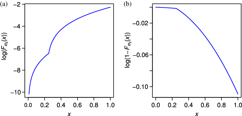
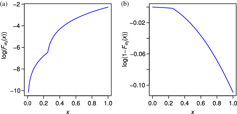
Example 5. Let
 $A( t)=t$
. We consider a decreasing scale function
 \begin{equation*} b( t) =2\,\mathds{1}_{[0,0.25)}( t) +1\,\mathds{1}_{[0.25,\infty)}( t) . \end{equation*}
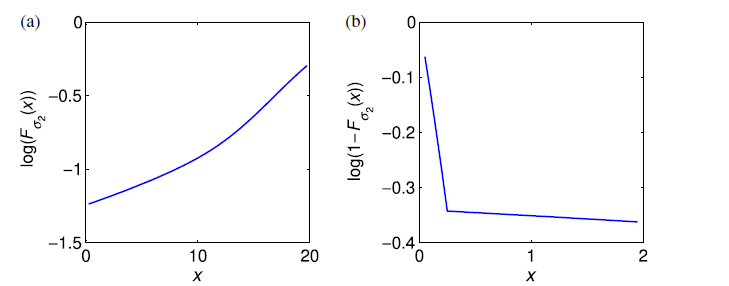
As can be seen in Figure 3 (a), the function
 $\log({F}_{\sigma_{2}}) $
is not concave and hence
 $\sigma_{2}$
is not DRHR. In Figure 3 (b), we can note that the function
 $\log(\bar{F}_{\sigma_{2}}) $
is concave and hence
 $\sigma_{2}$
is IFR. This is consistent with the result of Corollary 2.
Plots of
 $\log({F}_{\sigma_{2}}) $
and
 $\log(\bar{F}_{\sigma_{2}}) $
for
 $A( t)=t$
and
 $b( t) =2\,\mathds{1}_{[0,0.25)}( t) +1\,\mathds{1}_{[0.25,\infty)}( t) $
.
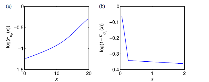
Example 6. Let
 $A( t)=t$
. We now consider an increasing scale function
 \begin{equation*} b( t) =0.1\,\mathds{1}_{[0,0.25)}( t) +10\,\mathds{1}_{[0.25,\infty)}( t) . \end{equation*}
As can be seen in Figure 4 (a),
 $\log({F}_{\sigma_{2}}) $
is not concave and hence
 $\sigma_2$
is not DRHR. In addition, we can observe in Figure 4 (b) that the function
 $\log(\bar{F}_{\sigma_{2}}) $
is not concave and hence
 $\sigma_{2}$
is not IFR.
Plots of
 $\log({F}_{\sigma_{2}}) $
and
 $\log(\bar{F}_{\sigma_{2}}) $
for
 $A( t)=t$
and
 $b( t) =0.1\,\mathds{1}_{[0,0.25)}( t) +10\,\mathds{1}_{[0.25,\infty)}(t) $
.
5. Recap and perspectives
Stochastic comparisons and ageing properties have been found, considering an EGP as a model for cumulative deterioration in reliability theory. Note that the results can naturally be used in other contexts such as finance or risk theory.
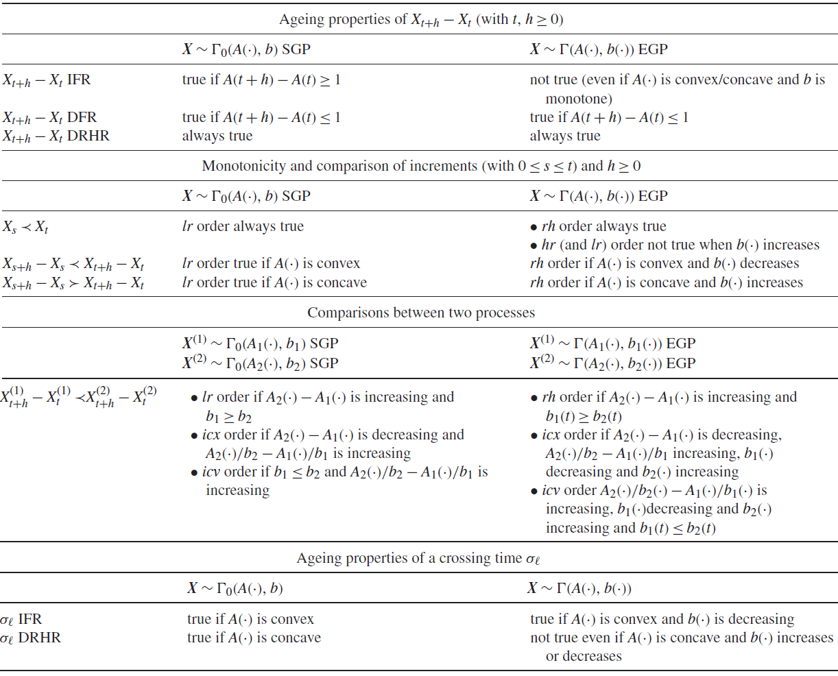
Most of the results of the paper are summed up in Table 1, where previous results for SGPs are recalled for comparison with their extended version (EGPs). Note that the comparison results between an SGP and an EGP from Corollary 1 and Proposition 7 do not appear in this table, for better readability.
Ageing properties and stochastic ordering for SGPs (second column) and EGPs (third column)
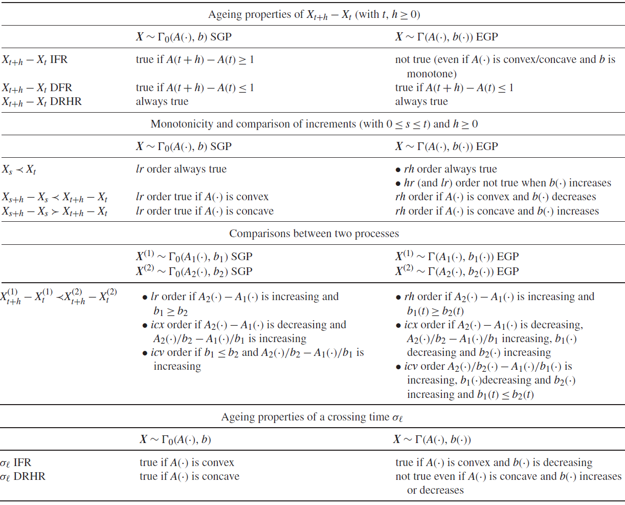
As can be seen in Table 1, the results previously obtained for SGPs and dealing with the DFR/DRHR property of an increment remain true. Those dealing with
 $icx/icv$
comparison results and the IFR property of a crossing time have a natural extension, adding a monotonicity assumption on the scale function(s) of the EGP(s). However, we can note that the lr (and hr) results for SGPs do not remain valid considering EGPs, and only results with the weaker rh order have been obtained (with counterexamples showing that the results cannot be extended to the lr order in most cases). Also, we remind the reader that we have not been able to conclude whether
 $X_{s}\prec_{\textrm{lr}}X_{t}$
for
 $s < t$
could be valid assuming the shape function to be convex or concave and the scale function to be increasing (see Remark 2). This (challenging) question hence remains open.
Clearly there remain many other stochastic orders (and ageing properties) to be investigated in the context of an EGP, such as the stochastic precedence order [Reference Boland, Singh and Cukic3], for which one might hope to obtain results under weaker conditions than for the usual stochastic order studied in this paper, or for more technical stochastic orders such as (harmonic) mean residual life order, dispersive order, excess wealth order, convex order, to cite only a few. (We refer to the seminal books quoted in the Introduction, where the interested reader can find further stochastic ordering and ageing notions, for which the degree of importance may vary according to the application context.) Hence there remain many investigations needed for better understanding of the possible stochastic behavior of an EGP, even restricting the study to the domain of stochastic comparisons and ageing properties.