





1. Introduction
Only a few exact solutions are known for the surface-elevation profile and the velocity field of glaciers, ice streams and ice sheets (e.g., Nye, Reference Nye1952, Reference Nye1965; Böðvarsson, Reference Böðvarsson1955; Vialov, Reference Vialov1958; Halfar, Reference Halfar1981; Bueler and others, Reference Bueler, Lingle, Kallen-Brown, Covey and Bowman2005; Bueler, Reference Bueler2014). Most of these solutions address steady-state problems and target the steady surface-elevation profile of ice sheets (e.g., Vialov, Reference Vialov1958) or the steady ice flow field for given idealised bed geometries (e.g., Nye, Reference Nye1952). Some of them also describe the time-dependent evolution of synthetic ice-flow problems (e.g., Halfar, Reference Halfar1981; Bueler and others, Reference Bueler, Lingle, Kallen-Brown, Covey and Bowman2005). Although these solutions require various simplifying assumptions, they provide valuable insight into the geometry and flow of natural ice masses. For example, the exact profile of Vialov (Reference Vialov1958), derived for a constant-width, constant-accumulation and non-sliding ice sheet resting on a flat bedrock, worked reasonably well for an observed surface-elevation profile in East Antarctica (Cuffey and Paterson, Reference Cuffey and Paterson2010). Exact solutions are also very useful in testing and benchmarking numerical schemes for solving glacier dynamics (e.g., Bueler and others, Reference Bueler, Lingle, Kallen-Brown, Covey and Bowman2005).
Several of the above exact solutions deal with idealised steady, time-independent problems. From empirical observations and model simulations, any given mountain glacier may be hypothesised to attain such a steady state if the climate forcing were to remain steady over a period much longer ( $ \gt rsim 5$ times) than its (climatic) response time scale of decades to centuries (Oerlemans, Reference Oerlemans2001). Oerlemans (Reference Oerlemans1984) argued that over much longer time scales of
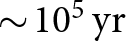 $\sim\!10^5\,\mathrm{yr}$, subglacial erosion significantly lowers the bedrock, causing glaciers to shrink due to the associated negative mass-balance feedback. In contrast, continuous rock uplift, e.g., due to tectonic processes, would cause glaciers to grow because of a positive mass-balance feedback loop. Thus, a stable long-term glacier cover requires either continuous rock uplift or persistent climate cooling to compensate for the effects of subglacial erosion (Oerlemans, Reference Oerlemans1984). This suggests the possibility that, wherever both occur, the competing processes of glacial erosion and rock uplift may stabilise a steady-state glacier cover over long time scales. It was recently shown that such a long-term steady-state glacier cover can indeed be realised in the limit of steady climate and constant and uniform rock uplift, when the subglacial erosion rate is proportional to the product of the local ice flux and the surface slope (Banerjee and Scherler, Reference Banerjee and Scherler2025). An exact Gaussian solution for the surface-elevation distribution, or equivalently, the hypsometry of such a steady glacier was obtained for a linear mass-balance profile (Banerjee and Scherler, Reference Banerjee and Scherler2025). Here, we exploit the above steady-state surface-elevation distribution to seek a corresponding analytical solution for the steady-state surface-elevation profile of 1) mountain glaciers having a Gaussian width distribution, and 2) axisymmetric ice caps. The surface profile of a numerically simulated glacier, obtained using a flowline model incorporating rock uplift and subglacial erosion, is compared with the exact analytical form for the constant-width case.
2. Theory
2.1. Steady-state surface-elevation distribution
Following Banerjee and Scherler (Reference Banerjee and Scherler2025), consider a glacier having a linear mass-balance  $(b)$ profile as a function of elevation
 $(z)$,
 \begin{equation}
b(z)=\beta (z-E),
\end{equation}
with  $\beta$ and
 $E$ denoting the mass-balance gradient and equilibrium-line altitude (ELA), respectively. The ELA is taken to be a constant that does not vary with space or time.
Take the subglacial erosion rate  $\epsilon$ at any given location to be proportional to the product of the local ice flux per unit width and the surface slope, i.e., the local streampower associated with the ice flow (Deal and Parsicek, Reference Deal and Prasicek2021; Hergarten, Reference Hergarten2021; Banerjee and Scherler, Reference Banerjee and Scherler2025):
 \begin{equation}
\epsilon=\alpha s q.
\end{equation}
Here, the ice flux per unit width  $q$ is the product of the local ice thickness and the depth-averaged ice flow speed, and
 $s\doteq|\frac{dz}{dx}|$ is the slope of the ice surface, with
 $x$ denoting the downglacier distance along the central flowline. The empirical erodibility parameter
 $\alpha$ relates the subglacial erosion rate to the local streampower associated with the flow of ice. The streampower is a measure of the potential energy lost per unit area and unit time due to the downslope flow. Equation (2) is a simplified form of a known scaling rule, which approximates the microscopic physics of erosion (Deal and Parsicek, Reference Deal and Prasicek2021; Hergarten, Reference Hergarten2021). The present theory assumes the scaling exponents associated with
 $q$ and
 $s$ to be one (Banerjee and Scherler, Reference Banerjee and Scherler2025). This choice is consistent with available data on landscape-scale glacial erosion rates (Banerjee and Scherler, Reference Banerjee and Scherler2025), and makes the problem analytically tractable. See sect. 3.3 for more discussion on the erosion rule.
The surface-elevation distribution or hypsometry of the glacier  $a(z)$ is the distribution of glacier surface area with elevation, such that the area in the interval
 $(z, z + \delta z)$ is given by
 $a(z)\delta z$, where
 $\delta z \gt 0$. It was previously shown (Banerjee and Scherler, Reference Banerjee and Scherler2025) that if
 $a(z)$ were to remain steady under a competition between rock uplift
 $\mathcal{U}$ and glacial erosion
 $\epsilon$, then it takes a Gaussian form. This was derived in Banerjee and Scherler (Reference Banerjee and Scherler2025) starting from the following steady-state continuity equation for the hypsometry under competing rock uplift and glacial erosion (Banerjee and Scherler, Reference Banerjee and Scherler2025):
 \begin{equation}
\mathcal{U}\frac{da}{dz}-\frac d {dz}(\epsilon a)=0.
\end{equation}
The glacier area in the elevation range  $(z,z+\delta z)$ is by definition
 $a(z)\delta z$. Denoting the length of the corresponding segment of the central flowline by
 $\delta x$, the same area is also given by
 $\delta x \times w(z)$, so that
 $a\delta z=w\delta x $. Now, for a glacier flowing in the positive
 $X$-direction, the local surface slope is
 $-\delta z/\delta x$. In the limit of
 $\delta x\rightarrow 0$, this implies,
 \begin{equation}
\frac wa=-\frac{dz}{dx}.
\end{equation}
Combining Eqs. 1, 2 and 4, and assuming a steady-state conservation of ice mass to express the total ice flux as an integral of the product  $ab$ over the range from
 $z_{max}$ to
 $z$,
 $\epsilon$ is eliminated from Eq. 3 to obtain an ordinary first-order differential equation for
 $a$,
 \begin{equation}
\frac{da}{dz}=-\frac{\alpha}{\mathcal{U}}ab.
\end{equation}
This can be integrated from  $z=E$ with boundary condition
 $a(z=E)=a_E$ to obtain,
 \begin{equation}
a(z)= a_E e^{-\frac{(z-E)^2}{2 \sigma^2}},
\end{equation}
where  $\sigma\doteq\sqrt{{\mathcal{U}} /(\alpha \beta)}$. The steady hypsometry is a Gaussian centred at the ELA, and it has a standard deviation of
 $\sigma$ in the limit of
 $(z_{max}-E)\gg\sigma$, where
 $z_{max}$ is the elevation of the top of the glacier. This elevation-range parameter of the hypsometry
 $\sigma$ is determined by the rock-uplift rate
 ${\mathcal{U}}$, the bedrock erodibility
 $\alpha$ and the mass-balance gradient
 $\beta$. Note that
 $\mathcal{U}$ is taken to be a constant that does not vary with space or time.
2.2. Steady-state elevation profile
With the steady-state Gaussian form (Eq. 6) for the hypsometry  $a(z)$ and any given
 $w(z)$, Eq. 4 can be integrated to obtain the following steady-state relation between the longitudinal coordinate and surface elevation:
 \begin{equation}
-\int_{x_E}^x dx' = x_E-x = a_E \int_E^z \frac 1 {w(z')} e^{-\frac{(z'-E)^2}{2\sigma^2}} dz',
\end{equation}
where  $x_E$ denotes the position of the ELA. Computing the above integral for a given
 $w(z)$ to obtain
 $x(z)$ analytically or numerically, and then inverting it for
 $z(x)$ yields the steady-state elevation profile. Below, we discuss some interesting solutions for the steady-state elevation profile.
2.2.1. A glacier with a Gaussian width distribution
A convenient choice for  $w(z)$, motivated by the empirical fact that glaciers tend to be wider near the ELA, is a Gaussian centred around the ELA, i.e.,
 \begin{equation}
w(z)= w_E e^{-\frac{(z-E)^2}{2 \nu^2}},
\end{equation}
where,  $w_E$ denotes the glacier width at the ELA, and
 $\nu$ is the standard deviation of the Gaussian. Inserting this into Eq. 4 yields,
 \begin{equation}
\frac{w_E}{a_E} e^{\frac{(z-E)^2}{2\bar\sigma^2}}=-\frac{dz}{dx}.
\end{equation}
Here, we consider the case  $\nu \gt \sigma$, and define
 $\tilde\sigma \doteq \sigma/ \sqrt(1-\frac{\sigma^2}{\nu^2})$. Denoting the magnitude of the surface slope at the ELA by
 $s_E\doteq-\frac{dz}{dx}|_{x=x_E}$, and using Eq. 4, we get
 $w_E/a_E=s_E$. Substituting this into the above equation, and integrating,
 \begin{equation}
x_E -x= \frac{\sqrt 2 \tilde\sigma} {s_E} \int_0^{\frac{z-E}{\sqrt 2 \tilde\sigma} }e^{-z'^2} dz' = \frac{\sqrt 2 \tilde\sigma}{s_E} \times \frac{\sqrt \pi} 2 \,\text{erf}\left(\frac{z-E}{\sqrt 2 \tilde\sigma}\right).
\end{equation}
In the second relation above, we use the definition of the error function  $\mathrm{erf(x)}\doteq\frac2{\sqrt\pi}\int_0^x e^{-x'^2} dx'$. Note that for a finite
 $z_{max}$, it requires an appropriate ice flux at the top of the glacier, e.g., due to avalanching from the headwall, such that there is a finite erosion rate at the top of the glacier.
Finally, utilising the corresponding definition of the inverse error function, the exact solution for the steady elevation profile of the glacier is written as,
 \begin{equation}
z(x)= E+\sqrt 2\tilde\sigma \,\text{erf}^{\,-1}\left( \sqrt \frac 2 {\pi}\frac{s_E(x_E-x)}{\tilde\sigma}\right).
\end{equation}
This exact solution depends on the parameters  $E, s_E,$ and
 $\tilde\sigma$, with the latter parameter determined in terms of
 $\nu$ and
 $\sigma$. The parameters
 $ \alpha, \beta$ and
 ${\mathcal{U}} $ only appear through the elevation-range parameter
 $\sigma\doteq\sqrt{{\mathcal{U}} /(\alpha \beta)}$ of the Gaussian hypsometry (Eq. 6), which has the dimension of length. In the limit of
 $\nu \rightarrow\infty$, that is, for a glacier having a constant width
 $w_E$ at all elevation bands,
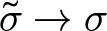 $\tilde\sigma\rightarrow\sigma$. In this limit, the above solution reduces to,
 \begin{equation}
z(x)= E+\sqrt 2\sigma \,\text{erf}^{\,-1}\left( \sqrt \frac 2 {\pi}\frac{s_E(x_E-x)}{\sigma}\right).
\end{equation}
Note that for the case  $\nu \lt \sigma$, integrating Eq. 4 leads to analogous exact solutions for
 $x(z)$ that involve imaginary error functions. When
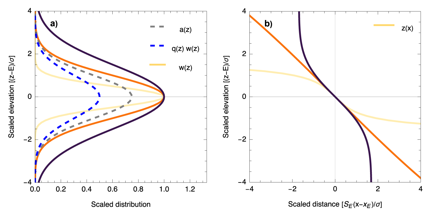
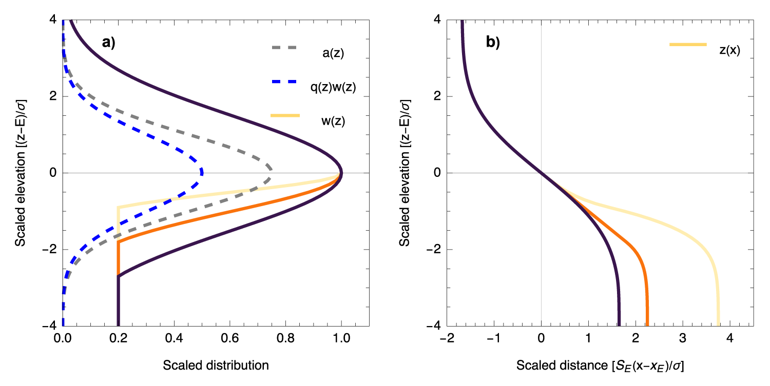
 $\sigma=\nu$, the steady profile is a straight line. The shapes of several steady elevation profiles are shown in Fig. 1 for specific choices of
 $\sigma$,
 $\nu$ and
 $s_E$.
Steady-state glacier elevation profiles obtained by numerically integrating Eq. 4 for three different choices of Gaussian width-distribution functions (Eq. 8). (a) Gaussian hypsometry  $a(z)$ with standard deviation
 $\sigma$ (grey dashed line), Gaussian width distribution
 $w(z)$ with standard deviation
 $\nu$ (solid yellow, orange and black lines denoting the three choices for
 $\nu/\sigma=$ 0.5, 1.0 and 1.5, respectively), and the total ice-flux distribution
 $q(z) w(z)$ are plotted against scaled elevation measured from ELA. The distributions are normalised arbitrarily to avoid overlap. (b) The steady ice-surface elevation profiles (yellow, orange and black solid lines) corresponding to each of the width distributions are shown. The curve for the case
 $\nu=1.5\sigma$ (black solid line) represents the inverse error function solution (Eq. 11).

2.2.2. An axisymmetric ice cap
For a cylindrically symmetric ice cap, denoting the radial distance from the symmetry axis by  $r$, Eq. 4 has the following form because
 $w(r)=2\pi r$:
 \begin{equation}
2 \pi r a(z)^{-1}=-\frac{dz}{dr}.
\end{equation}
Integrating the above equation with  $a(z)$ from Eq. 6,
 \begin{equation}
(r^2-r_E^2)=-\sqrt {2 \pi}~\frac{r_E \sigma}{s_E} \text{erf}\left(\frac{z-E}{\sqrt 2 \sigma}\right).
\end{equation}
Note that for this axisymmetric problem, the slope at  $z=E$ satisfies
 $s_E= \pi r_E a_E^{-1}$. Inverting the above equation, the following elevation profile for the steady-state ice cap is obtained:
 \begin{equation}
z(r)= E+\sqrt 2\sigma \,\text{erf}^{\,-1}\left( \sqrt{\frac 1 {2 \pi}}\frac{s_E(r_E^2-r^2)}{r_E\sigma}\right).
\end{equation}
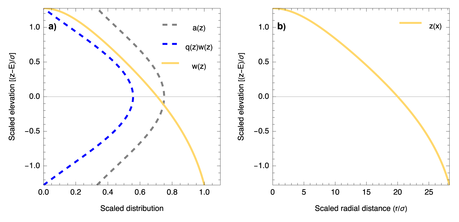
The corresponding radial profile is plotted in Fig. 2, where the lowest elevation is where the ice flux goes to zero.
Note that the above derivation for the axisymmetric case suggests the possibility for a class of exact steady-state profiles  $z(x)$ applicable to mountain glaciers. Equation 4 can be solved in a similar manner as above to obtain the corresponding exact profile
 $z(x)$, whenever the width distribution of a mountain glacier is a given function
 $x$ such that the integral
 $\int^x_{x_E} w(x')dx'$ is known analytically.
Steady-state elevation profile of an axisymmetric ice cap. (a) Gaussian hypsometry  $a(z)$ (grey dashed line), the corresponding total ice-flux distribution
 $q(z)w(z)$ (blue dashed line) and the width distribution
 $w(z)=2 \pi r(z)$ (solid yellow line) shown as a function of scaled elevation measured from ELA. The distributions are normalised arbitrarily to avoid overlap. (b) The exact solution (Eq. 15) for the radial ice-surface elevation profile of an axisymmetric ice cap (solid yellow line) is plotted. Here, we chose the location of the ELA to be
 $r_E= 20 \sigma$, and the surface slope at the ELA to be
 $s_E=0.1$.

3. Discussion
3.1. Properties of the steady glacier
3.1.1. Steady-state extent
As the error function is bounded between 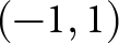 $(-1,1)$, the exact solution (Eq. 10) implies that the terminus of the steady glacier is at
 $x\approx x_E+\sqrt{\frac \pi 2} \tilde\sigma/s_E$ to a good approximation as long as
 $\tilde\sigma\ll (z_{max}-E)$. Therefore, in this limit, the length of the steady glacier is given by,
 \begin{equation}
L \approx \sqrt{2\pi}\frac{\tilde\sigma}{s_E}.
\end{equation}
Apart from an expected inverse slope dependence (e.g.,
Bahr and others, Reference Bahr, Meier and Peckham1997), the length is proportional to the elevation-range parameter  $\tilde\sigma$. Furthermore, the steady glacier has the same elevation range above and below the ELA, with the elevation range controlled by the same parameter
 $\tilde\sigma$. As
 $\tilde\sigma \doteq \sigma/ \sqrt(1-\frac{\sigma^2}{\nu^2})$, for a fixed value of
 $\sigma$, glaciers with relatively larger
 $\nu$ will have shorter length (Fig. 2). Note that the present theory does not provide any insight into the geological or climatic controls on the free parameters
 $\nu$ and
 $s_E$, if any such controls exist.
The limit of  $\nu\rightarrow\infty$ corresponds to a constant-width glacier, for which
 $\tilde\sigma$ approaches
 $\sigma$ and the elevation range directly reflects a competition between rock uplift and subglacial erosion. For a higher mass-balance gradient (which implies a higher ice flux), or for a higher erodibility, the erosion rates are relatively higher, and this causes a decline in the length and elevation range of the glacier. On the other hand, a higher rock uplift increases the length and elevation range. We emphasise that this discussion refers to the long-term (
 $\sim10^5-10^6$ yr) steady-state extent of the glacier, and not to the century-scale steady state for a given uniform climate. In the latter case, the relatively slow evolution of the bedrock can be safely ignored.
The elevation-range parameter  $\sigma$ for constant-width glaciers controls both the length and the slope of the exact solution. It is determined by the combination
 $\sigma\doteq\sqrt{{\mathcal{U}}/(\alpha \beta)}$ of the three input parameters, such that the fractional change in the long-term steady length and elevation range is half of the fractional changes in any of these three parameters. For example, a 10% increase in erodibility
 $\alpha$ or mass-balance gradient
 $\beta$ leads to a 5% reduction in glacier length and elevation range. Similarly, a 10% increase in uplift rate
 ${\mathcal{U}}$ leads to a 5% increase in the length and elevation range of the steady glacier. This, for example, implies that if the slope and the mass-balance gradients are comparable, longer glaciers with higher elevation ranges may be expected in regions with relatively higher rock uplift rates or lower bedrock erodibility. In fact, a similar association between elevation range and uplift rate has been empirically shown, with the elevation ranges of glacierised mountains around the world being systematically higher for regions with relatively higher rock uplift rates (Pedersen and others, Reference Pedersen, Egholm and Nielsen2010). Note that in the limiting case of
 ${\mathcal{U}}\rightarrow0$, the steady solution represents a horizontal, and therefore static, slab of ice with its surface elevation exactly matching the ELA.
3.1.2. Shape of the steady-state profile
While derived under idealised assumptions, the inverse error-function form for the steady-state elevation profile of the idealised glacier (Eq. 11) has some similarities with the observed morphological characteristics of mountain glaciers. The exact solution for the surface-elevation distribution  $a(z)$ (Eq. 6) has a maximum at the ELA, i.e., at
 $z=E$. Equation (8) shows that the elevation with the most gentle glacier surface slope is also at
 $z=E$. A shallow surface slope and the surface-elevation distribution peaking at the ELA are reminiscent of global-scale observations relating the hypsometric peak in glacial landscapes with the long-term regional snowline elevation (Egholm and others, Reference Egholm, Nielsen, Pedersen and Lesemann2009). Furthermore, the exact steady-state profile (Eq. 11) has an inflection point at the location of the peak of the elevation distribution
 $x=x_E$, where the surface profile makes a transition from a concave-up to a convex-up shape. Such an inflection of the glacier surface has long been used to estimate the so-called ‘kinematic’ ELA of any given glacier (Leonard and Fountain, Reference Leonard and Fountain2003, and references therein). Interestingly, the numerical solution for the steady profile for
 $\sigma/\nu=2$ has a concave-up (convex-up) accumulation (ablation) zone (Fig. 1b). However, this may not be a physically relevant solution, as the length of such a glacier with an inverse imaginary error function form has an infinite length.
The functional form of the steady-state solution (Eq. 11) implies that it is antisymmetric about the ELA, i.e.,  $z(-\Delta x+x_E)-E= E- z(\Delta x+x_E)$. However, for real mountain glaciers with a possibly weaker mass-balance gradient in the accumulation zone (e.g.,
Oerlemans, Reference Oerlemans2001) and an asymmetric width distribution, the above symmetry is unlikely to exist. This can be seen in the numerical examples in Fig. 3, where the slope of the ablation zone is reduced for steady glaciers with a relatively narrower ablation zone. In this figure, the chosen width distributions mimic real glaciers that often have an approximately constant width in their lower ablation zone. The step-like drop at the terminus (Figs. 1b and 3b) is a feature of the exact solution which may be specific to the idealised glaciers. For real glaciers, the sharp decay of the Gaussian elevation distribution near the terminus is likely to be accompanied by a steep reduction in width, which would likely smooth the steep section. Also, a variable climate would most likely cause the terminus to fluctuate around the steady-state position, which would modify this section of the bedrock.
Examples of steady-state glacier elevation profiles for three different choices of non-Gaussian, asymmetric width distribution functions. (a) Gaussian hypsometry  $a(z)$ (grey dashed line), the corresponding total ice flux distribution
 $q(z)w(z)$ (blue dashed line) and the three chosen asymmetric width distributions
 $w(z)$ with a constant width in the lower ablation zone (solid lines) are shown as a function of scaled elevation measured from ELA. Three chosen examples of the width distributions are shown as yellow, orange and black lines, and are ordered so that warmer colours have relatively narrower ablation zones. The distributions are normalised appropriately for the ease of visualisation. (b) The corresponding steady ice-surface elevation profiles are shown with coloured solid lines, with colours denoting the width of the ablation zone. These solutions are obtained by numerically integrating Eq. 4.

3.1.3. Short-term mass-balance sensitivity to ELA change
Based on the steady-state conservation of ice mass, the net balance of a glacier is given by the integral of the mass-balance profile, weighted by the normalised surface-elevation distribution or hypsometry  $a(z)$ of the glacier (e.g.,
Oerlemans, Reference Oerlemans2001). For the above steady-state glacier with a Gaussian elevation distribution (Eq. 6) and a linear mass-balance profile (Eq. 1), this integral is easy to solve analytically, and yields a vanishing steady-state mass balance,
 $\int_{-z_{max}}^{z_{max}} a(z)\beta(z-E) = 0$ as expected.
When an abrupt instantaneous rise in ELA,  $E\rightarrow E+\Delta E$, is applied to this steady glacier, the instantaneous (annual) net balance
 $\bar{b}$ can also be calculated analytically as,
 \begin{equation}
\bar{b}=\int_{-z_{max}}^{z_{max}} a(z) \times \beta(z - E - \Delta E)\,dz = - \beta \Delta E.
\end{equation}
For a realistic case, where the ELA fluctuates around its steady-state climatological value on an interannual scale, the above expression for the net balance  $\bar{b}$ suggests that the ELA vs the annual mass balance plot has a slope of
 $-\beta$. For real glaciers, such plots are routinely used to estimate mass balance from remotely observed end-of-summer snowline, a proxy for the ELA (e.g.,
Rabatel and others, Reference Rabatel2017). The mass-balance sensitivity to ELA change, which is the slope of such a regression line, therefore exactly equals the negative mass-balance gradient (
 $-\beta$) for the idealised glacier considered here. This is consistent with the corresponding empirical results for real glaciers that are available in the literature (Raper and Braithwaite, Reference Braithwaite and Raper2009, and references therein).
A consequence of the steady surface-elevation distribution (Eq. 6) being symmetric about the ELA is that the accumulation-area ratio (AAR) exactly equals  $1/2$ for the steady state. Note that the AAR is the ratio of the accumulation area to the total glacier area (e.g.,
Rabatel and others, Reference Rabatel2017). Again, the AAR can be computed analytically for an instantaneous rise in ELA by
 $\Delta E$—simply by integrating the normalised hypsometry (Eq. 6) over the elevation range (
 $E+\Delta E, z_{max}$),
 \begin{align}
\text{AAR} & = \frac 1 2 \left (1 - \frac{\text{erf}({\Delta E}/{\sqrt 2\tilde\sigma})} {\text{erf}\left({(z_{max}-E)}/{\sqrt 2\tilde\sigma}\right)}\right)\nonumber\\
& \approx \frac 1 2 \left(1 - \sqrt{\frac{2}{\pi}} \frac{\Delta E}{\tilde\sigma} + \mathcal{O}(\frac{\Delta E^3}{\tilde\sigma^3})\right).
\end{align}
Here, in the second relation, we linearise the error function about  $z=E$ in the limit of
 $\Delta E \ll \tilde\sigma$, and ignore terms involving
 $\exp \left(-{(z_{max}-E)^2}/(2\tilde\sigma^2)\right)$ assuming that
 $(z_{max}-E)\gg\tilde\sigma$. Eliminating
 $\Delta E $ from the above equation with the help of Eq. 17 and rearranging, one obtains a linear relationship between the AAR and the annual mass balance
 $\bar{b}$ as follows:
 \begin{equation}
\bar{b} = \sqrt{2\pi}\beta \tilde\sigma (\text{AAR}-\text{AAR}_0).
\end{equation}
Here AAR $_0$ denotes the steady-state AAR value, which is 1/2 for the present exact solution. This relationship is analogous to the empirical
 $\bar{b}$-AAR relationship that is routinely used to estimate the annual mass balance
 $\bar{b}$ from the lowest extent of the accumulation zone, typically derived from the end-of-summer snowline altitude. For ballpark values of
 $\beta\sim10^{-2}$ yr
 $^{-1}$ and
 $\tilde\sigma\sim 10^2$ m, the proportionality constant in Eq. 19
 $\sqrt{2\pi} \beta \tilde\sigma\approx2.5$ m yr
 $^{-1}$, which is comparable to the corresponding empirically determined values available in the literature, e.g.,
 $\sim2.3$ m yr
 $^{-1}$ in Kulkarni (Reference Kulkarni1992), and
 $\sim 3.7$ m yr
 $^{-1}$ in Rabatel and others (Reference Rabatel2017).
3.1.4. Erosion-uplift balance
Combining Eqs. 2 & 4, the erosion rate at any elevation  $z$,
 $\epsilon(z)= \alpha w q/a$. Now, from the conservation of ice mass for a steady glacier,
 $wq= q(z_{max}) w(z_{max})+\int_z^{z_{max}}a b dz'$, where the first boundary term represents possible ice flux into the glacier at the headwall, for example, due to avalanching. The second term can be evaluated for a Gaussian form of
 $a(z)$ and a linear mass-balance profile (Eqs. 6 & 1) to obtain,
 \begin{equation}
\epsilon(z) = \frac {\alpha q(z_{max}) w(z_{max})} {a(z)}+ \mathcal U \left(1-\frac{a(z_{max})}{a(z)} \right),\\
\end{equation}
where we used that  $\alpha\beta \sigma^2=\mathcal{U}$. Now, assuming a specific boundary condition at the top that the erosion rate there is related to the boundary ice flux via the streampower erosion rule (Eq. 2), the expression for the erosion rate can be simplified further. The steady-state condition for the ice-free bedrock at the top then requires
 $\mathcal{U} =\alpha s(z_{max}) q(z_{max}) = \alpha w(z_{max}) q(z_{max}) /a(z_{max})$. This implies, the boundary term
 $\alpha q(z_{max}) w(z_{max}) /a(z) = \mathcal{U} a(z_{max})/a(z)$, and therefore, Eq. 20 simplifies to,
 \begin{equation}\epsilon(z)=\mathcal{U},\end{equation}
such that the mean erosion rate is a constant equal to the uplift at all elevation bands. While this is the case for the exact solution 12, this does not necessarily mean that any steady-state glacier profile must satisfy Eq. 21. For example, in the numerical example discussed below, where a no-flux boundary condition at the top of the glacier is assumed, the erosion rate is elevation-dependent at the steady state.
3.2. Comparison with simulated constant-width glacier
To compare the above exact analytical solution for the constant-width glacier (Eq. 12) with a corresponding numerically simulated steady profile, we use our previous implementation (Banerjee and Scherler, Reference Banerjee and Scherler2025) of a standard flowline model for a constant-width glacier (Oerlemans, Reference Oerlemans2001). We ignore the flow due to ice deformation, and assume that the flow is dominated by sliding with the sliding speed  $u_s=f_s \rho^3 g^3 H^2 s^3$, where
 $\rho$ is the density of ice,
 $g$ is the gravitational acceleration,
 $H$ is the ice thickness, and the sliding parameter
 $f_s=2.4\times10^{-20}\,\mathrm{Pa^{-3}m^{-2}s^{-1}}$ (Oerlemans, Reference Oerlemans2001). The model uses mass-balance gradient of
 $\beta=0.0071\,\mathrm{yr}^{-1}$ and ELA of
 $E=4752$ m. These two model parameter values, and the remaining ones given below, are chosen from a corresponding range suitable for Himalayan glaciers using a random number generator (Banerjee and Scherler, Reference Banerjee and Scherler2025). The bedrock undergoes subglacial erosion following Eq. 2, with bedrock erodibility
 $\alpha=9.6\times10^{-6}$ m
 $^{-1}$, and experiences rock uplift at a rate of
 ${\mathcal{U}}=8.9\times10^{-3}$ m yr
 $^{-1}$ (Banerjee and Scherler, Reference Banerjee and Scherler2025). An explicit finite-difference scheme is employed to integrate the model over
 $10^6$ yr, with time and space steps of
 $0.5 \times 10^{-3}$ yr and 30 m, respectively. A no-flux boundary condition is imposed at the top boundary. The ice-free parts of the bedrock are assumed to erode by river incision following a stream power model, where the incision rate is proportional to the product of the local bedrock slope and the distance from the head of the catchment (e.g.,
Anderson and Anderson, Reference Anderson and Anderson2010). The corresponding proportionality constant is set to
 $\kappa=4.2\times10^{-6}$ m
 $^{-1}$ (Banerjee and Scherler, Reference Banerjee and Scherler2025), and the initial ice-free fluvial bedrock is taken to be a logarithmic steady river profile for the given rock uplift rate
 ${\mathcal{U}}$ and fluvial erodibility parameter
 $\kappa$ (e.g.,
Anderson and Anderson, Reference Anderson and Anderson2010),
 \begin{equation}
z(x)=z(x_0)-\frac {\mathcal{U}} {\kappa} \ln \frac{x-x_0}{x_0}.
\end{equation}
To avoid numerical instabilities, the ice surface and the ice-free bedrock are both smoothed by a three-site moving average once every 1000 time steps.
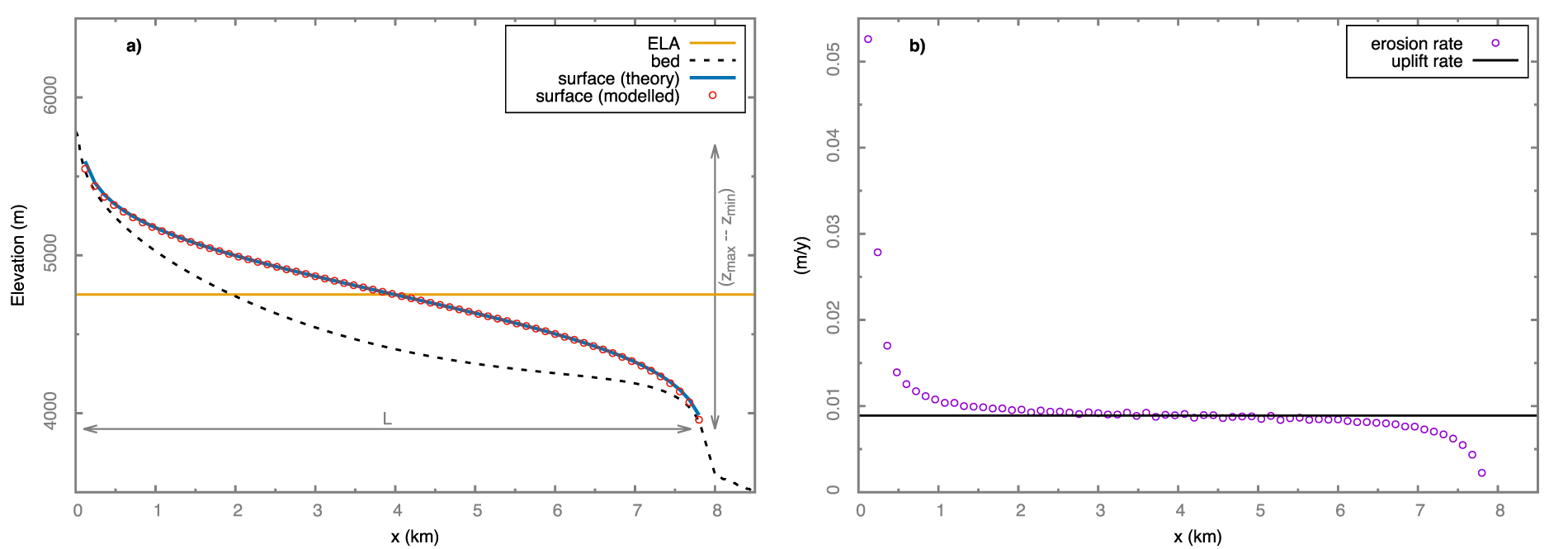
As is evident from Fig. 4, the analytical steady-state solution (Eq. 12) provides a fairly accurate description of the final steady-state elevation profile of the modelled flowline glacier at  $t=10^6$ yr without any curve-fitting. The exact solution is plotted using the same values of the input parameters
 $\alpha, \beta$ and
 $\mathcal{U}$, and
 $E$ as used in the simulation, and the modelled values of
 $x_E \text{and }s_E$. The simulation also produces the steady bedrock and ice-thickness profiles (Fig. 4a), given the ice-flow rule adopted (See Sect. 3.3). There are some small, but systematic deviations between the modelled and theoretical surface elevation profile near the top and the terminus of the glaciers. These are related to the finite elevation range of the modelled glacier and the zero-flux boundary condition used at the top boundary. Note that the simulated steady-state glacier does not satisfy Eq. 21, and the erosion rate at the steady state is elevation dependent (Fig. 4b).
(a) The exact solution (Eq. 12) for the ice-surface elevation (solid blue line) matches well the simulated steady-state elevation profile (open red circles), without any curve fitting. The ELA (solid orange line) and the steady bedrock-elevation profile (dashed black line) are shown. The length of the glacier  $L$ and its elevation range
 $(z_{max}-z_{min})$ are marked with grey arrows. (b) The modelled uplift and erosion rate profile of the steady-state glacier.

3.3. Scope of the exact theory
The exact elevation profiles presented in the manuscript are calculated assuming a steady-state Gaussian hypsometry (Eq. 6). This was derived in Banerjee and Scherler (Reference Banerjee and Scherler2025) starting from (A) a steady-state continuity equation for the hypsometry under competing rock uplift and glacial erosion, along with the assumptions of (B) a linear mass-balance profile (Eq. 1) and (C) a streampower-dependent bedrock erosion rule (Eq. 2). The streampower was computed assuming (D) a steady-state conservation of ice mass to express total ice flux as an integral of the product  $ab$ over the range from
 $z_{max}$ to
 $z$. As long as the above four assumptions are valid, the steady-state elevation profile is obtained by solving the ordinary differential equation (Eq. 4) for any given form of
 $w(z)$. The examples worked out here (Eqs. 11 & 12) assume a Gaussian or constant
 $w(z)$. For the steady axisymmetric ice cap (Eq. 15), the width is a linear function of the radial distance (Sect. 2.2).
Apart from the four assumptions listed above, additional assumptions can be added to the present theory to estimate other quantities of interest. For example, the above theory does not refer to any specific parametrisation of the deformation and/or the sliding of glacier ice. Assuming a suitable ice-flow rule, one can compute, either analytically or numerically, the corresponding steady profiles of surface velocity, ice thickness, bedrock elevation, etc. For example, our flowline model simulation (Sect. 3.2) assumes ice flow by basal sliding, with the sliding speed  $u_s$ computed as
 $f_s H^2 s^3$, where a factor of
 $\rho^3 g^3$ is subsumed into
 $f_s$ for convenience. Therefore, the ice flux per unit width is given by
 $q= u_s H =f_s H^3 s^3$. From the conservation of ice mass (volume), the flux per unit width
 $q(z)=\int_z^{\infty}a b /w \,dz = \frac {\beta \tilde\sigma^2}{\sqrt{2\pi}s_E} e^{-\frac {(z-E)^2}{2 \tilde\sigma^2}}$, where we use Eqs. 3, 7 & 8 and take the limit
 $z_{max}\rightarrow\infty$ to simplify the calculations. Combining these two expressions and using Eq. 4, one obtains a Gaussian ice-thickness profile as follows:
 \begin{equation}
H(z)=f_s^{-1/3}s^{-1} q^{1/3} =\left (\frac{\beta\tilde \sigma^2}{\sqrt{2\pi}f_s s_E^{4}} \right)^{\frac 1 3} e^{-\frac {2 (z-E)^2}{3 \sigma^2}}.
\end{equation}
As both the surface-elevation profile (Eq. 12) and ice-thickness profile (Eq. 22) are known, their difference gives the subglacial bedrock profile. The above ice-thickness profile, along with the slope profile  $s(z)=s_E e^{\frac {(z-E)^2}{2 \tilde\sigma^2}}$ (Eq. 8), obtains the sliding velocity profile as
 $u_s(z)\sim e^{\frac {(z-E)^2}{6 \tilde\sigma^2}}$. The profile of sliding speed essentially mimics that of the slope, with a minima at the ELA and diverging values away from the ELA, but has a relatively weaker variation with elevation
 $z$.
The analytical solutions for the steady hypsometry, surface elevation, ice thickness and bedrock may be useful in testing numerical models for the evolution of glacial landscapes, as long as the model satisfies the assumptions A–D listed above. The exact surface-elevation profile (Eqs. 10 & 12) will hold independent of the parametrisation used to model the ice flow, e.g., a shallow-ice formulation of ice deformation, plastic flow and/or a parametrisation of basal sliding (Oerlemans, Reference Oerlemans2001; Cuffey and Paterson, Reference Cuffey and Paterson2010). Of course, the ice-thickness and bedrock profiles need to be recalculated in each case, based on the slope and thickness dependence of the flux per unit width. The present exact theory will not apply to models that use an erosion law that is different from Eq. 2, e.g., a power-law scaling of erosion rate with sliding velocity, or a more general streampower-based scaling rule of the form  $\epsilon \sim q^m s^n$, with
 $m\neq1$ and
 $n\neq1$ (Deal and Parsicek, Reference Deal and Prasicek2021; Hergarten, Reference Hergarten2021). In such cases, the present solution could still be relevant if the erosion rate has an approximately linear dependence on the product
 $q s$, over the range of modelled erosion rates (Banerjee and Scherler, Reference Banerjee and Scherler2025).
A complication ignored in the present theory is that subglacial erosion is related to the sliding of ice (e.g.,
Herman, Reference Herman, De Doncker, Delaney, Prasicek and Koppes2021). As a result, the erosion rule (Eq. 2) has limited applicability for non-sliding, cold-based ice e.g.,
Hergarten (Reference Hergarten2021), where all the ice flow is by deformation. However, if the cold-based condition is prevalent only for parts of a glacial-interglacial cycle, this formulation may still apply over longer time scales, with an appropriate reduction of the effective erodibility constant  $\alpha$, to reflect the non-erosive conditions for certain parts of the climate cycle. Also, the present theory estimates the erosion rate (Eq. 2) using ice flux computed using a steady-state mass-conservation argument, and therefore, it ignores any variation in the relative contributions of basal sliding and ice deformation to the ice flow. Within the present erosion rule (Eq. 2), such a variation effectively makes the erodibility spatially variable, e.g.,
 $\alpha\sim (1 + \frac {f_d}{f_s} H^2 )$ within a shallow-ice flowline model incorporating both sliding and deformation (Oerlemans, Reference Oerlemans2001), where
 $f_s$ and
 $ f_d$ are the parameters governing sliding and deformation, and
 $H$ is the spatially varying ice thickness. Therefore, a constant
 $\alpha$ as considered here is strictly valid only in the thin-ice limit when
 $H^2 \ll \frac{f_d}{f_s}$.
While some properties of the exact solution for the idealised steady glacier are comparable to the corresponding observed characteristics of real glaciers, any direct quantitative application of the exact solution to real glaciers in nature is complicated by the spatial and temporal variability of the rock uplift, climate forcing and bedrock erodibility across a range of scales. All these factors are assumed to be spatially homogeneous and temporally uniform in the derivation of the steady-state exact solution. For real glaciers, transients due to time-dependent climate forcing and/or rock uplift may mask any potential signals of the long-term steady balance. Transient numerical simulations using 1D or 2D landscape-evolution models can further help understanding the implications of our approach and the exact solutions for real glacial landscapes—particularly, the transient effects of climate cycles.
4. Conclusions
A steady-state exact solution for the elevation profile of an idealised mountain glacier on an erodible bedrock is presented, assuming a steady competition between subglacial erosion and rock uplift. This steady-state solution has an inverse error-function form, which is derived for a time-independent and spatially uniform rock uplift, a linear mass-balance profile, a streampower-dependent subglacial erosion rule and a steady Gaussian glacier width distribution. The solution does not involve any assumptions about the nature of the ice flow mechanisms or about the form of the bedrock. The exact surface-elevation profile has an inflection point at the ELA, and is antisymmetric about the ELA. In the constant-width limit, the elevation range of the steady glacier is determined by the elevation scale  $\sigma\doteq\sqrt {{\mathcal{U}}/(\alpha\beta)}$, which increases with the rock uplift and decreases with erosional efficiency, with the latter factor controlled by the bedrock erodibility
 $\alpha$ and the mass-balance gradient
 $\beta$. For the steady glacier, an instantaneous change in ELA causes proportionate changes in the net mass balance and the AAR of the glacier, both of which are computed analytically. The steady exact elevation profile is also derived for an axisymmetric ice cap.
Data availability statement
The C code used to simulate the flowline glacier on erodible bedrock is publicly available (Banerjee and Scherler, Reference Banerjee and Scherler2025), and the relevant model data and gnuplot codes used to make the figures are available on https://github.com/ab-glac/exact_prof.
Acknowledgements
We acknowledge input from Eric Deal and thank reviewers Ed Bueler and Martin Lüthi for critical comments, all of which helped to improve the content and clarity of the manuscript.
Author contributions
A.B. conceived the theory, did the analytical and numerical calculations and wrote the manuscript. D.S. contributed to the discussions and edited the manuscript.








 Open access

