





Impact Statement
This paper raises awareness regarding good benchmarking practices in system identification and discusses a newly introduced results-reporting platform together with baseline identification results for a selected set of nonlinear system identification benchmark datasets.
1. Introduction
Nonlinear dynamics are observed in a wide range of applications and are well studied in the electrical, mechanical, and biomedical engineering research fields and beyond. Nonlinear system identification aims to obtain models of these nonlinear dynamics starting from measured data. Although the development of nonlinear system identification approaches has already a long history, their importance continues to grow due to increasing performance demands on engineering systems (e.g., improved energy efficiency or improved positioning accuracy), combined with the growing complexity of the systems under consideration. As nonlinear dynamics refer to everything that is not linear, a wide range of model structures and identification approaches have been developed to cover the broadest possible range of nonlinear dynamics (Schoukens and Ljung, Reference Schoukens and Ljung2019; Nelles, Reference Nelles2020).
Even though the goal of system identification is to obtain models of dynamic systems starting from (noisy) data, a surprisingly low percentage of publications thoroughly compare newly proposed approaches on publicly available datasets. This can be explained by the wide diversity of systems, applications, constraints, and model end goals that are being considered during identification tasks. On top of this, publicly available implementations of the proposed identification algorithms were often missing in the systems and control community (Zhou et al., Reference Zhou, Brunke, Tao, Hall, Bejarano, Panerati and Schoellig2024). Only recently has the use of public Git repositories to share algorithm implementations started to become commonplace. This contributed to the observation that, in contrast with some machine learning and image-processing research fields (see, e.g., ImageNet [Deng et al., Reference Deng, Dong, Socher, Li, Li and Fei-Fei2009] and WikiText [Merity et al., Reference Merity, Xiong, Bradbury and Socher2016] for image and language processing, respectively), no strong benchmarking and comparison culture has been present within the research fields involved with system identification. Although multiple datasets have been collected and published in recent decades (De Moor et al., Reference De Moor, De Gersem, De Schutter and Favoreel1997; Wigren and Schoukens, Reference Wigren and Schoukens2013; Kroll and Schulte, Reference Kroll and Schulte2014; Schoukens and Noël, Reference Schoukens and Noël2017; Gilpin, Reference Gilpin2021), new identification approaches are most often illustrated in ad hoc simulation examples, with limited comparison to other methods.
The comparison of approaches is important for the development of the field, as it highlights promising research directions and offers a clear answer to practitioners on what type of identification approach provides the best performance for a given problem at hand. However, due to the diversity of nonlinear dynamic systems, experimental conditions, and end-use applications (control, system design, structural health monitoring, validation and certification, etc.), a wide range and diversity of benchmark datasets are required too. It is not uncommon for a given identification approach to be among the best for a certain application in a given experimental condition, while performing only mediocre in a different one.
When reporting benchmark results, it is essential to be able to place these results into context. Hence, having a wide range of baseline and state-of-the-art results available on a single benchmark problem is important. To compare approaches, clear guidelines on how to split the available data in training/validation/test and calculate the selected figures of merits should be available. However, an open platform to report this information for nonlinear system identification tasks is not present within the community. This means that the obtained results are scattered throughout the literature. This is to the detriment of newly published approaches that may omit comparisons to methods not proposed within a certain subfield.
The present paper introduces an open benchmark result-reporting platform for a selected set of benchmark problems through the nonlinearbenchmark.org website and tools to enhance the accessibility to the benchmarking process found in github.com/MaartenSchoukens/nonlinear_benchmarks. The present paper also reflects on the role of benchmarks within our community, and on how to report benchmark results. Furthermore, a broad set of baseline results have been generated on these benchmark problems using well-established model structures and methods. These results should offer a firm base to position new result submissions within the established literature. The full flow from benchmark selection to result reporting as hosted on nonlinearbenchmark.org is visualized in Figure 1.
Nonlinearbenchmark.org hosts the full benchmarking flow starting from a broad range of benchmark systems over a standardized data loader, to results reporting and a leaderboard.

Figure 1. Long description
A thick light blue arrow points from left to right, serving as the baseline for five sequential stages.
1. Benchmark system. A photo of a vertical laboratory apparatus with tubes and mechanical components.
2. Data loader. Two stacked line graphs labeled Train and Test, showing fluctuating signal data over a horizontal axis from 0 to 1000.
3. Identification. An icon of a lightbulb with a gear inside, flanked by two smaller gears.
4. Testing and figure of merit. A large black checkmark icon.
5. Results submission. A digital form with text fields for Email, Author names, Method name, Link to paper/technical report, and Link to code repository.
6. Leaderboard. A spreadsheet-style table titled Benchmark Results, containing columns for Date submitted, Author names, Method, Paper/Technical Report, Code, and Score.
The final blue arrow head points toward the right edge of the frame, indicating the completion of the flow.
In the remainder of this paper, Section 2 provides a selected overview of the available nonlinear system identification benchmark datasets and a reflection on the different goals of benchmarking in nonlinear system identification and discusses the role of figures of merit in comparing methods. Section 3 introduces the nonlinearbenchmark.org benchmark hosting and result-reporting platform. Finally, some baseline results are obtained on the selected benchmark problems in Section 4.
2. Benchmarking in system identification
2.1. Goals of benchmarking
2.1.1. Why do we benchmark?
A first advantage of benchmarking is the performance assessment of a developed approach. Furthermore, if the chosen benchmark datasets cover relevant challenges in the field, obtaining good results on these benchmarks establishes the credibility of the proposed approach. Finally, when using widespread benchmarks, the competitiveness of the proposed approach can be established and validated at a low cost for the authors, as many other results on the same data will be available in the literature. This bypasses the time-consuming task of implementing and running other approaches on the examples one wants to compare. Finally, a well-constructed benchmark can also raise the attention of open challenges in the research field.
2.1.2. What constitutes a good benchmark?
A good benchmark problem consists of many different components. A clear overview of the main elements involved is provided by Reddi (Reference Reddi2024, Chapter 11): standardized datasets, predefined tasks, evaluation metrics, baseline results, reproducibility, and results interpretation guidelines. In the next paragraphs, we revisit these aspects and briefly discuss them from a system identification point of view.
2.1.3. Standardized datasets
Data forms the starting point of most identification algorithms. To be able to compare multiple identification methods, the same data should be used. Preferably, these datasets should match the wide variety of data encountered in engineering practice ranging from low to high signal-to-noise ratios, from short (expensive) to long (cheap) experiments, and from highly informative to less informative experiments. However, starting from a fixed dataset ignores the important input/experiment design aspect of the system identification cycle. Hence, we should also accommodate benchmark systems where custom datasets can be generated.
2.1.4. Predefined tasks and evaluation metrics
The end goal of a model is often not the model itself, but, for example, the design of a controller, a structural health monitoring, or a predictive maintenance tool. Nevertheless, if we want to provide a comparison of identification algorithms, a clearly defined task needs to be specified. In system identification tasks, this is often minimizing the (Root) Mean Square Error (RMSE), or a normalized variation of it (e.g. the best-fit rate), between the actual measured outputs and the predicted or simulated output. In some cases, some distance between the actual system parameters (e.g., resistor and capacitor values in an electric network) and the estimated model parameters are considered, but this significantly restricts the model structures that can be used as it should be closely tied to the considered nature of the parameters.
At the same time, the RMSE is often used as the main quantitative evaluation metric. However, focusing on such a metric alone would be damaging to the general development of the field as it ignores a wide array of qualities that can be incorporated by a method or by the identified model and the algorithm used to estimate it: e.g., the model and algorithmic complexity, the robustness of the algorithm, uncertainty quantification, or the computational demand for the estimation and the use of the model. Clearly, one needs to leave room for nuance and detailed explanation of the reported results to account for a wide range of user demands due to various end uses of an estimated model. Examples of such considerations include, for instance, the recent awareness regarding “green AI” and “green-box” system identification: e.g., a model that has a 10% higher error but that can be obtained with only 1% of the computational cost can be highly relevant for a wide range of applications (Batselier, Reference Batselier2022; Memmel et al., Reference Memmel, Menzen, Schuurmans, Wesel and Batselier2024).
2.1.5. Result interpretation
As argued earlier, comparing identification approaches on a limited number of figures of merit only (e.g., RMSE), would not be effective. The end use of the model often adds additional constraints. Hence, when interpreting results, the qualitative description of the benefits and limitations of an approach is paramount. Furthermore, benchmark problems only cover a limited set of the full problem space. Focusing only on benchmark results would bias the field too much toward a (limited) set of (nonlinear) system identification problems.
2.1.6. Baseline results
Including baseline results and their implementations provides a key idea of what minimum performance should be expected, and what the classical tools within the field can obtain. An obvious baseline result for nonlinear system identification could, for instance, be the result of a linear model. Any nonlinear model performing worse than this is most likely of little interest to the community. At the same time, these baselines limit the danger of cherry-picking the approaches one compares with when they aim to publish their results. As the baselines are published together with the benchmark data or are very visible, reviewers will also have easy access to them.
2.2. Available datasets and benchmark systems: A selected overview
The DaISy database (De Moor et al., Reference De Moor, De Gersem, De Schutter and Favoreel1997) is one of the earlier websites that hosted a wide range of system identification datasets. The database covers a wide range of systems, mainly coming from the process industry (glass furnace, stirring tank, power plant) and mechanical systems (CD player, wing flutter, flexible robot arm) application areas. These DaISy datasets come with a brief (1 paragraph) description and typically are limited to several hundred up to 2000 data points.
The MATLAB System Identification Toolbox (Ljung, Reference Ljung2024) also includes several datasets such as a Magneto-Rheological Fluid Damper, a Two-Tank system, and a Motorized Multi-Axle Camera. These datasets are often provided to illustrate Matlab’s built-in (nonlinear) system identification capabilities. As such, clear example scripts are provided on how to work with these datasets.
Furthermore, multiple datasets and benchmark system simulators have been proposed as benchmark problems and were the topic of invited sessions at international conferences and workshops. Examples of these include the Wiener-Hammerstein (Schoukens and Ljung, Reference Schoukens and Ljung2009), Silverbox, Cascaded Tanks and Coupled Electric Drives (Wigren and Schoukens, Reference Wigren and Schoukens2013), Cantilever Beam (Tiso and Noël, Reference Tiso and Noël2017), Cascaded Tanks with Overflow, Wiener-Hammerstein with Process Noise, and Bouc-Wen Hysteretic datasets (Schoukens and Noël, Reference Schoukens and Noël2017), F-16 Ground Vibration Test dataset (Noël and Schoukens, Reference Noël and Schoukens2020), and 2-Story Frame simulator (Vlachas et al., Reference Vlachas, Tatsis, Agathos, Brink and Chatzi2021).
Other datasets have been collected and published as part of a research project and been considered as relevant benchmark datasets. Examples of these include the Cortical Responses Evoked by Wrist Joint Manipulation dataset (Vlaar et al., Reference Vlaar, Solis-Escalante, Vardy, van der Helm and Schouten2017, Reference Vlaar, Birpoutsoukis, Lataire, Schoukens, Schouten, Schoukens and van der Helm2018) and a 4-DOF motion ship dataset (Baier and Staab, Reference Baier and Staab2022), as well as the more recent Hawk T1A Modal Testing dataset (Haywood-Alexander et al., Reference Haywood-Alexander, Mills, Champneys, Bonney, Wagg and Rogers2023; Haywood-Alexander et al., Reference Haywood-Alexander, Mills, Champneys, Jones, Bonney, Wagg and Rogers2024).
Finally, some previous publications collected a wide set of benchmark datasets and simulators (Kroll and Schulte, Reference Kroll and Schulte2014) or focused on a specific type of system dynamics, e.g., chaotic systems (Gilpin, Reference Gilpin2021) or fluid dynamics (Towne et al., Reference Towne, Scott, Brès, Lozano-Durán, Saxton-Fox, Parthasarathy, Jones, Biler, Yeh, Patel and Taira2023).
Unfortunately, all the datasets and systems listed previously are limited to hosting or publishing data. The results obtained for each dataset are difficult to retrieve from the literature as no central reporting repository is available. Hence, making a detailed comparison between methods remains challenging.
3. Nonlinearbenchmark.org: A platform for nonlinear system identification benchmark datasets
The nonlinearbenchmark.org website features multiple datasets obtained from a wide range of nonlinear dynamical systems. Several of these are more regularly used for demonstration than others; these are typically single-input single-output systems and datasets with a richer input. The present paper considers seven of the most widely used benchmark datasets among those to demonstrate the proposed results-reporting flow, from standardized data loading to the result submission portal, together with the obtained baseline model results.
3.1. Datasets
The present paper considers the following lab-scale benchmark systems (Figure 2): the Silverbox (Wigren and Schoukens, Reference Wigren and Schoukens2013) which mimics a Duffing oscillator/Fitz-Nagumo model, the Electro-Mechanical Positioning System (Janot et al., Reference Janot, Gautier and Brunot2019), which exhibits friction behavior, the Wiener–Hammerstein (WH) system (Schoukens and Ljung, Reference Schoukens and Ljung2009) containing a saturation nonlinearity between two linear time-invariant (LTI) blocks, as well as a parallel WH system that has a high dynamical complexity as it consists of two parallel WH signal paths (Schoukens et al., Reference Schoukens, Marconato, Pintelon, Vandersteen and Rolain2015), the cascaded tanks (CT) system (Schoukens et al., Reference Schoukens, Mattsson, Wigren and Noël2016; Schoukens and Noël, Reference Schoukens and Noël2017) with overflow nonlinearities, the coupled electric drives (CED) (Wigren and Schoukens, Reference Wigren and Schoukens2017) wherein only the absolute value of the velocity is measured, and the F-16 ground vibration test dataset (Noël and Schoukens, Reference Noël and Schoukens2020), which contains highly resonant dynamics with shifting resonant peaks for increasing forcing amplitudes. A brief description of each of the systems is provided later; a detailed description can be found in the provided references.
Overview of the considered benchmark systems: (a) Silverbox, (b) Wiener–Hammerstein, (c) Parallel Wiener–Hammerstein, (d) Cascaded Tanks, (e) Coupled Electric Drives, (f) F-16 Ground Vibration Test, and (g) Electro-Mechanical Positioning System.

Figure 2. Long description
The panels are organized as follows.
* Panel a. A feedback control block diagram. Input u enters a summing junction with a positive sign. The forward path contains a block with the transfer function 1 all over (m s squared plus c s plus k sub 1). The output y feeds back through a block labeled k sub 3 y cubed to the negative terminal of the summing junction.
* Panel b. A block diagram with three stages. Stage G sub 1 shows a low-pass filter frequency response. Stage f[.] shows an electrical circuit with resistors and a diode. Stage G sub 2 shows a frequency response with a sharp notch.
* Panel c. A parallel block diagram. Two parallel paths each contain three blocks. The first blocks show low-pass curves, the second blocks show high-pass curves, and the third blocks show notch filters. Both paths converge at a summation symbol.
* Panel d. A photo of a vertical experimental setup with two transparent cylindrical tanks mounted on a white board with connecting tubes.
* Panel e. A schematic of a mechanical drive system. It features a P C for real-time control connected to an A D / D A converter, an anti-aliasing filter, and a power amplifier. These drive two motors connected by a flexible belt to a pulley with a pulse transducer and a spring.
* Panel f. A photo of an F-16 fighter jet inside a hangar, supported by testing equipment for ground vibration analysis.
* Panel g. A photo of a horizontal electro-mechanical positioning system with a long lead screw, a sliding carriage, and a control interface at the base labeled d S P A C E.
All these benchmark datasets provide the user with a predefined measured dataset. This has the advantage of offering a clearly defined task and facilitates comparison between approaches. However, it also limits the use of the benchmarks for evaluating the downstream use of the model, as the true system is not available for evaluating downstream results of the identification, such as control design or health monitoring, nor can they be used for other system identification challenges, such as input design or active learning.
3.1.1. Wiener–Hammerstein (WH)
The Wiener–Hammerstein system class is a well-known block-oriented structure (Schoukens and Tiels, Reference Schoukens and Tiels2017). It contains a static nonlinearity that is sandwiched in between two LTI blocks. As the signal that governs the nonlinear behavior is not directly measured (it is hidden by the two LTI blocks), this results in a problem that is harder to identify, e.g., input–output representations such as NAR(MA)X models.
The Wiener–Hammerstein benchmark (Schoukens and Ljung, Reference Schoukens and Ljung2009) was the subject of an invited session during the IFAC Symposium on System Identification in St. Malo, France in 2009, and has attracted quite some attention since. The system is an electronic circuit with a Wiener–Hammerstein structure built by Gerd Vandersteen (Reference Vandersteen1997), where the nonlinearity is realized as a diode resistor network. It is excited by a highly informative input signal and features a low-noise, large 188,000 samples long measured dataset.
3.1.2. Parallel Wiener–Hammerstein (ParWH)
A Parallel Wiener–Hammerstein system is obtained by connecting multiple Wiener–Hammerstein systems in parallel. The system considered in this benchmark is an electronic circuit with a two-branch parallel Wiener–Hammerstein structure (Schoukens et al., Reference Schoukens, Marconato, Pintelon, Vandersteen and Rolain2015). The front and back LTI blocks of each branch are third order continuous-time IIR filters. The static nonlinearity of each branch is realized with a diode-resistor network. The measured training dataset is over 3 million data points large, containing measurements at 5 different amplitude levels, with multiple realizations of a random phase multisine input signal at each amplitude level (Schoukens et al., Reference Schoukens, Marconato, Pintelon, Vandersteen and Rolain2015; Schoukens, Reference Schoukens2020). Twenty realizations at each amplitude level can be used for training and validation, and one realization per amplitude level is available for testing. The aforementioned challenges in identifying a Wiener–Hammerstein model are further complicated due to its parallel branch nature and the increased order of the system dynamics (12th order).
3.1.3. Silverbox (SB)
The Silverbox system is an electronic implementation of a mass-spring-damper system with a cubic spring (Wigren and Schoukens, Reference Wigren and Schoukens2013). This is also sometimes known as a forced Duffing oscillator. However, the current benchmark is constructed such that it never enters a bifurcating regime: for the applied input signals, a fading memory behavior is observed. Similar to the Wiener–Hammerstein case, the Silverbox system has been widely studied in the literature, and this benchmark also offers highly informative data, in a low-noise setting, and a long data record. It can be considered as one of the “entry-level” benchmark problems that are considered here. The training dataset contains concatenated multisine realizations, while the testing dataset contains a multisine excitation and a random Gaussian noise input with growing amplitude experiment.
3.1.4. Cascaded Tanks (CTs)
The cascaded tanks system consists of two water tanks with free outlets fed by a pump (Schoukens et al., Reference Schoukens, Mattsson, Wigren and Noël2016). The input controls a water pump that delivers the water from a reservoir into the upper water tank. The water of the upper tank flows through a small opening into the lower tank, and finally through a small opening from the lower tank back into the reservoir. The water level of the lower tank is considered as the system output (measured in V using a capacitive sensor). This benchmark combines soft and hard (due to overflow) nonlinearities to be identified based on relatively short data records.
3.1.5. Electro-Mechanical Positioning System (EMPS)
The EMPS is a standard configuration of a drive system for prismatic joints of robots or machine tools (Janot et al., Reference Janot, Gautier and Brunot2019). The main source of nonlinearity is the friction effects that are present in the setup. Due to the presence of a pure integrator in the system, the measurements are obtained in a closed-loop setting.
3.1.6. Coupled Electric Drives (CEDs)
The CED system consists of two electric motors that drive a pulley using a flexible belt (Wigren and Schoukens, Reference Wigren and Schoukens2017). The pulley is held by a spring, resulting in a (lightly) damped dynamic mode. The drive control is symmetric around zero, hence both clockwise and counter-clockwise movements are possible. The angular speed of the pulley is measured as an output with a pulse counter, and this sensor is insensitive to the sign of the velocity. The available datasets are short, which presents a challenge when identifying a model.
3.1.7. F16 Ground Vibration Test (F16)
The F-16 Ground Vibration Test benchmark (Noël and Schoukens, Reference Noël and Schoukens2020) features a high-order system with clearance and friction nonlinearities at the mounting interface of the payloads. The experimental data made available were acquired on a full-scale F-16 aircraft on the occasion of the Siemens LMS Ground Vibration Testing Master Class, held in September 2014. During the test campaign, two dummy payloads were mounted at the wing tips to simulate the mass and inertia properties of real devices typically equipping an F-16 in flight. One shaker was attached underneath the right wing to apply input signals. The aircraft structure was instrumented with accelerometers. A preliminary investigation showed that the back connection of the right-wing-to-payload interface was the predominant source of nonlinear distortions in the aircraft dynamics, and is therefore the focus of this benchmark study. Measurements were performed using multisine and sinesweep experiments at 7 different amplitude levels each. Amplitude levels 1, 3, 5, and 7 are used for training and validation while the others are used for testing. Note that the “standardized dataset” used here only comprises the random phase multisine and sinesweep measurements; the odd multisine measurements are omitted as they cover a much broader frequency range. The standardized dataset also only considers the first of the three offered outputs in the dataset.
3.2. Improving data accessibility and data standardization
The presented datasets for nonlinear system identification have been collected by different researchers over multiple years. To enhance the accessibility of datasets, the present paper presents a Python toolbox available at github.com/MaartenSchoukens/nonlinear_benchmarks. Through this, we offer a unified method of downloading any of the desired datasets and a standardized data representation to the user, even when the underlying data representations are heterogeneous across benchmarks. For example, you can subsequently find a usage of the toolbox to download and load the previously mentioned Wiener–Hammerstein dataset.
-
1. import nonlinear_benchmarks as nlb #installed with “pip install nonlinear-benchmarks”
-
2. train_val, test = nlb.WienerHammerBenchMark() # automatically downloads dataset
-
3. sampling_time = train_val.sampling_time # in seconds
-
4. # Extract input signal u(t) and output signal y(t) as numpy arrays
-
5. u_train_val, y_train_val = train_val.u, train_val.y
-
6. u_test, y_test = test.u, test.y
-
7. n_ini = test.state_initialization_window_length
As seen in the example, the toolbox automatically splits the data into a default training and test set. It remains up to the user to split the training dataset further into train and validation, depending on the requirements of the identified algorithm considered. The test data cannot be used to make any estimate/decision during the modeling process. The test result can only be used to validate the final model quality. For some systems, multiple test and/or train records are considered, e.g., when the dataset consists of a list of measured data records, or to consider different operating regimes of the system.
The automatic data split also fixes the modeling problem, which was considered because many of the benchmark problems did not specify at their introduction what the precise modeling problem is or they offered multiple use cases in the spirit of flexibility: e.g., both the forward or the inverse modeling problem could be considered for the EMPS. However, when establishing leaderboards, this flexibility must be reduced to avoid confusion and offer a clear and fair comparison of results.
Furthermore, the Python functions provided also implement a standardized figure of merit calculation using the RMS value of the simulation error. A short section (with length
$ {n}_{\mathrm{ini}} $
 ) of the test data can be used to initialize the model (e.g., state initialization). This short record is also provided by the Python functionality. This prevents the reported errors from being dominated by transient responses of the model. Mathematically this results in:


where
$ N $
 is the total length of the test data,
$ {u}_k $
 ,
$ {y}_k $
 , and
$ {\hat{y}}_k $
 are the system input, output, and the simulated model output at sample
$ k $
 respectively, and
$ \Gamma $
 represents the model for which the RMS error needs to be computed. The data lengths
$ N $
 and
$ {n}_{\mathrm{ini}} $
 differ from one benchmark system to the other. The correct implementation of the model
$ \Gamma $
 and its evaluation in the test set remain the responsibility of the users of the benchmark dataset, for example:
-
1. from nonlinear_benchmarks.error_metrics import RMSE
-
2. # Compute RMSE on predictions after n_ini points:
-
3. n_ini = test.state_initialization_window_length
-
4. y_test_model = Gamma(model, test.u, test.y[:n_ini]) # Gamma is user-provided model
-
5. test_RMSE = RMSE(test.y[n_ini:], y_test_model[n_ini:]) # users should report this value
3.3. Results submission
Results are submitted through an online form that can be accessed from the benchmark website itself. The form collects different aspects of the submitted contribution:
Date submitted: To keep track of the chronology of submissions.
Authors: To credit the authors of the submission, as well as a means to contact them in case further questions arise from other benchmark users.
Method: The name of the approach that has been used.
Link to a paper/technical report: A detailed description of the approach that has been used. This can be a published article or a preprint.
Open source code: In view of reproducibility, a link to an open source implementation of the considered approach should be reported, preferably including a working script that uses the considered benchmark data.
Commit ID/SHA/hash: To be able to access the correct version of the submitted code.
Considered benchmark: The name of the benchmark dataset on which the results are obtained.
Test results (RMSE): The simulation error (free-run simulation) RMSE is chosen as an all-round figure of merit to compare approaches.
Training time: This refers to the amount of time required for the algorithm to obtain the model estimate. The approximate training time is reported to provide an idea of the computational complexity of the approach.
Training platform: Some information about the computational platform that has been used during training (e.g., type of CPU and/or GPU, amount of memory). Together with the training time, this gives a better idea of the computational demand of the proposed approach.
White- to-black-box Scale (1–10): The authors are invited to self-assess how much prior information has been used during the identification process of the reported results ranging from no prior knowledge (black-box) to a purely physics-based approach (white-box). Potential contributors are referred to Schoukens and Ljung (Reference Schoukens and Ljung2019) and Cross et al. (Reference Cross, Rogers, Pitchforth, Gibson, Zhang and Jones2024) to help them position their results on this scale.
Author remarks: Finally, the authors have access to an open field in which they can specify further considerations and nuances on the obtained results and considered identification approach. We believe this option is crucial to, for instance, take into account the huge diversity of end-goals of data-driven modeling.
The submitted results are screened by a moderator before they are uploaded to the website itself to ensure the quality of the results, e.g., nonlinear identification results that perform worse than the linear baselines are most likely without merit, but also the novelty of the results to avoid double reporting (e.g., similar results that have been obtained by almost identical methods).
4. Baseline approaches
In this section, the proposed baseline NLSI models are introduced. It is the intention of the authors to demonstrate baseline results on well-established and readily available methodologies from the literature. Here, models are applied “out-of-the-box” without significant modification or tailoring to each benchmark problem. This is motivated by a desire to showcase results that might be expected given a nonintrusive application of commodity algorithms. As is well known in the NLSI community, the most rigorous test of model performance is in free-running simulation (where only the initial conditions of the system output are observed) (Schoukens and Ljung, Reference Schoukens and Ljung2019). Therefore, all models are tested exclusively in simulation. In all cases, data normalization is applied, with the normalizing transformation calculated using the training data only. For neural network-based approaches, data is scaled onto the interval
$ \left[-1,1\right] $
 . For all other methods, a zero-mean, unit variance scaling is applied. All RMSE scores are computed on unseen testing data in the original coordinates of the benchmarks, discarding the first
$ {n}_{\mathrm{ini}} $
 points as described in Section 3.2. In the present paper, baseline NLSI models are compared for three common model classes. The first class is linear time-invariant models consisting of an LTI state-space model and LTI ARX model (autoregressive with exogenous inputs) (Ljung, Reference Ljung1999). The second class is auto-regressive (AR) models (Billings, Reference Billings2013), consisting of the aforementioned LTI ARX model, polynomial nonlinear ARX model (PNARX), Gaussian process NARX model (GPNARX), and multilayer-perceptron NARX model (MLP NARX). The third class is recurrent neural networks (RNNs) consisting of the multilayer perceptron finite impulse response model (MLP FIR), the RNN, the long-short term memory network (LSTM) and its optimized variant (OLSTM) and the gated recurrent unit (GRU) (Ljung et al., Reference Ljung, Andersson, Tiels and Schön2020). The models in each class are described later for the convenience of the reader.
4.1. Linear time-invariant
4.1.1. LTI SS
Discrete-time LTI state-space models have been commonly used for decades in the system identification literature. Here, LTI state-space models with an output error noise model are estimated:

where
$ {u}_t $
 is the input,
$ {x}_t $
 is the state, and
$ {\hat{y}}_t $
 is the modeled output at time
$ t $
 . The matrices
$ A $
 ,
$ B $
 ,
$ C $
 , and
$ D $
 are paramerized in a “free” form, that is, any element in the matrix is freely adjustable. The state-space models are estimated using the prediction error framework (ssest command in Matlab). The resulting nonlinear optimization problem is initialized using a subspace estimate (Ljung, Reference Ljung1999).
The means of the measured input and output training data are subtracted before estimating the LTI state-space models. Hence, minimizing the prediction error results in a Best Linear Approximation model of the systems considered, following the lines of Enqvist and Ljung (Reference Enqvist and Ljung2005) and Pintelon and Schoukens (Reference Pintelon and Schoukens2012). The resulting mean values of the input and output training data are part of the resulting model as they are respectively subtracted from and added to any validation or test input provided to the model and resulting model output.
The number of states considered by the LTI SS approach for each benchmark is reported in Table 1. The state order
$ {n}_x $
 is selected based on the provided benchmark system descriptions, except for the EMPS benchmark, where a grid search with validation dataset illustrated that
$ {n}_x=4 $
 resulted in significantly better results than
$ {n}_x=2 $
 or
$ {n}_x=5 $
 , and slightly better than
$ {n}_x=3 $
 . The F16 LTI state-space model is estimated using data that was 8x downsampled (using the Matlab downsample command). To report the results, the model data is upsampled back to the original sampling rate (using the Matlab interp command).
Number of states used by the LTI SS models considered in the present paper

Table 1. Long description
The table consists of two rows and eight columns.
Row 1 (Headers): The first cell is empty. The subsequent columns are labeled S B, E M P S, W H, C T, C E D, Par W H, and F 16.
Row 2 (Data): The first cell contains the variable n sub x. The corresponding values for the models are:
* S B: 2
* E M P S: 4
* W H: 6
* C T: 2
* C E D: 3
* Par W H: 12
* F 16: 20
4.1.2. LTI ARX
This model is described in more detail in the auto-regressive models subsection.
4.2. Auto-regressive models
Auto-regressive (AR) models (Ljung, Reference Ljung1999; Billings, Reference Billings2013) encompass a class of methods that generate predictions of output variables given previous (or lagged) values. Many variants of AR models are well established in the NLSI literature, generalizing the linear, output-only AR formulation to exogenous inputs (ARX), nonlinear systems (NARX), and moving-average noise processes (ARMA). A convenient general representation of nonlinear AR models from an estimation point-of-view is to consider the NARX form, which performs the explicit prediction of the subsequent time point
$ {\hat{y}}_t $
 as,

where
$ \Phi $
 is a static map from the lagged inputs and outputs to the predictions, and where
$ {n}_u $
 and
$ {n}_y $
 refer to the number of lagged inputs and outputs, respectively. This has the advantage of transforming the system identification procedure into a static regression problem, to which many standard approaches can be applied. A convenient method of working with AR type models is to construct the Hankel matrix of lagged inputs and outputs,

where
$ N $
 is the total number of temporal points in the data and
$ p=\max \left({n}_y,{n}_u\right) $
 . This formulation allows one to express the prediction model as
$ \mathbf{y}=\Phi (H) $
 , where the static function
$ \Phi $
 depends on the specific form of the auto-regressive model under consideration. An open problem in AR modeling is how to specify the number of lags
$ {n}_y $
 and
$ {n}_u $
 . A cross-validation approach is often cost-prohibitive due to the combinatorial nature of the lag structure problem. The approach taken in this work, for all AR models detailed later, is to choose the lag structure with the best score for a linear ARX model, evaluated by the Akaike information criterion (AIC) (Akaike, Reference Akaike1998 on a hold-out validation (not testing) set, up to a maximum value of
$ {n}_y,{n}_u=20 $
 (except in chases whereby
$ {n}_{\mathrm{ini}} $
 is less 20 in which case that value is used instead). The only exception is for the CED benchmark for which this approach selects a very sparse lag structure (
$ {n}_u=1,{n}_y=3 $
 ), likely due to the symmetric nonlinearity on the output resulting in a minima at zero (in the least-squares sense) for input signals with zero mean Schoukens and Noël (Reference Schoukens and Noël2017). To avoid disadvantaging the nonlinear models, the lag structure for this benchmark is set (arbitrarily) to
$ {n}_y,{n}_u=10 $
 for all AR baselines. The lag structures of the AR models reported in this study are collected and shown for the convenience of the reader in Table 2. The authors note that the lag structure selected by the MLP NARX model (MLP NARX in Table 2) differs slightly from all others (denoted as AR in Table 2) because of a different data normalizing strategy. The MLP NARX model was trained with data standardized to the interval
$ \left[-1,1\right] $
 (as is standard practice for neural network training), whereas all other AR models were trained with data normalized to zero-mean and unit variance.
Lag structures used by the AR models considered in the present paper

Table 2. Long description
The table consists of eight columns and five rows.
Column headers from left to right are: Model Type, S B, E M P S, W H, C T, C E D, Par W H, and F 16.
Row 1: n sub u (A R) values are 14, 5, 12, 11, 10, 12, and 13 respectively.
Row 2: n sub y (A R) values are 7, 6, 6, 2, 10, 5, and 1 respectively.
Row 3: n sub u (M L P N A R X) values are 5, 5, 20, 20, 10, 9, and 6 respectively.
Row 4: n sub y (M L P N A R X) values are 2, 6, 20, 7, 10, 20, and 7 respectively.
4.2.1. LTI ARX
The first auto-regressive model considered here is the LTI auto-regressive with exogenous inputs (ARX) model. This is a linear formulation with,

where
$ \alpha $
 is an unknown vector of linear weights that can be evaluated by the solution of the linear equation
$ \mathbf{y}= H\alpha $
 . Many solvers are appropriate for this task. The results in the present paper use a QR-decomposition-based approach.
4.2.2. pNARX
The first nonlinear ARX (NARX) model considered in this study is the classical polynomial NARX model (Billings, Reference Billings2013). Here, the nonlinearity is defined as a linear combination of polynomial terms
$ {P}_n $
 computed from
$ H $
 :

To promote stability, only univariate polynomial terms are retained, that is, each basis function depends on a single regressor only, and cross-terms such as
$ {y}_{t-1}^2{u}_{t-1} $
 are excluded. A Legendre orthogonal polynomial basis up to order
$ n $
 is applied to each regressor independently to improve numerical conditioning. Concretely, for a single row
$ {h}^{\top }=\left[{y}_{t-1},\dots, {y}_{t-{n}_y},{u}_t,\dots, {u}_{t-{n}_u+1}\right]\in {\mathrm{\mathbb{R}}}^r $
 of
$ H $
 (with
$ r={n}_y+{n}_u $
 ), the feature map is

Where
$ {\mathrm{\ell}}_k $
 is the
$ k $
 th term in the Legendre basis, so that
$ \Phi (H)\in {\mathrm{\mathbb{R}}}^{N\times rn} $
 , and
$ \alpha \in {\mathrm{\mathbb{R}}}^{rn} $
 . The order of the polynomial is selected based on AIC cross-validation scores on the hold-out validation set, up to a maximum order of 10. The identified model orders are reproduced in Table 3 for the convenience of the reader. It is expected that the inclusion of multinomial terms may improve the identification on some benchmarks. However, a full multinomial basis leads to a very high number of basis terms for only a modest number of lags and so is not considered here.
Polynomial orders used by the PNARX models considered in the present paper

Table 3. Long description
The table consists of two rows and eight columns.
Row 1 (Header): The first cell is empty. The subsequent headers from left to right are S B, E M P S, W H, C T, C E D, Par W H, and F 16.
Row 2 (Polynomial order):
- S B: 7
- E M P S: 3
- W H: 5
- C T: 3
- C E D: 2
- Par W H: dash (no value)
- F 16: 2
4.2.3. GP NARX
Another common choice for the nonlinearity in NARX models is to use a Gaussian process (GP) model. GPs offer flexible kernel regression and quantification of uncertainty with few hyperparameters (Rasmussen and Williams, Reference Rasmussen and Williams2006). The nonlinearity is therefore,

The GP is entirely parametrized by the kernel function
$ K $
 and the mean function
$ m $
 . In this study, GP NARX models are constructed with a squared-exponential kernel and zero-mean function. Training GPs requires the specification of several kernel hyperparameters
$ {\theta}_K=\{{\sigma}_n^2,{\sigma}_f^2,\ell \} $
 . By convention, these are optimized by minimization of the negative-log marginal-likelihood with respect to the training data (Rasmussen and Williams, Reference Rasmussen and Williams2006). For a zero-mean GP, this is given by,

with
$ \Sigma =K\left(H,H\right)+{\sigma}_n^2I $
 , for the proposed noise variance term
$ {\sigma}_n^2 $
 .
Here, this is achieved with the well-known stochastic gradient descent algorithm ADAM (Kingma and Ba, Reference Kingma and Ba2014). For each benchmark, the hyperparameters are optimized from random initializations for a total of 1000 steps with a learning rate of
$ {10}^{-2} $
 . The hyperparameters with the best score on the hold-out validation set are then used for evaluation of the test set.
Due to the computational cost (
$ \mathcal{O}\left({n}^3\right) $
 for
$ n $
 datapoints) of training GPs, for benchmark sets with more than 1000 examples (EMPS, WH, SB, ParWH, F16), only the first 1000 points of the training set are used to train the model. For training on larger sequences, sparse GP approaches (such as those in Titsias, Reference Titsias2009; Hensman et al., Reference Hensman, Fusi and Lawrence2013) could be applied; however, these are not considered in this work following our philosophy of producing only “baseline” results to which more complex approaches can be compared.
4.2.4. MLP NARX
The final nonlinearity considered for NARX models in this study is to use a multilayer perceptron (MLP) for
$ \Phi $
 . Here, an MLP with a single hidden layer and hyperbolic tangent activation functions is considered. The number of nodes in the hidden layer is selected by cross-validation in the hold-out validation set with sizes of 2, 4, 8, 16, and 32 considered. Lags are selected by cross-validation of an ARX model by the procedure described earlier. Each network is trained for
$ {10}^4 $
 iterations of the ADAM (Kingma and Ba, Reference Kingma and Ba2014) optimizer, with 5 random initializations except for the two smallest benchmark datasets (CED and CT), which are optimized for
$ 2\times {10}^4 $
 iterations. The overall best network is selected as the one with the best score on the hold-out validation set. This network is then used for evaluation on the unseen testing set.
4.3. Recurrent neural-networks
In recent years, the field of NLSI has benefited greatly from significant developments in the realm of ML. In particular, recurrent neural network (RNN) models have gained a lot of attention within the system identification community and variants have generated impressive results on challenging benchmarks. RNNs approximate the evolution of dynamic systems by propagating a hidden “memory” state (or states) forward through the time evolution of the network.
This extends the standard MLP formulation to enable dynamical systems to be modeled in an input–output fashion. It is common when training RNNs to stack lagged values of the inputs up to a certain look-back distance. This can be achieved in a similar way to the AR models by constructing the Hankel matrix of the input values only. The network is then trained to predict the value of the output and the next sampling instant from the lagged inputs and the previous value of the hidden memory state.

Where
$ \mathbf{F} $
 is the forward pass of the neural network and
$ {n}_u $
 is the look-back distance. In the RNN literature,
$ \mathbf{F} $
 is often called a recurrent cell. Complex RNN models are often comprised of many such cells composed in series and parallel.
Although many advanced architectures have been proposed in a NLSI context (Beintema et al., Reference Beintema, Toth and Schoukens2021; Forgione and Piga, Reference Forgione and Piga2021b), the objective of the present paper is to compare baseline results for standard architectures; as such, this study considers only models with a single recurrent cell.
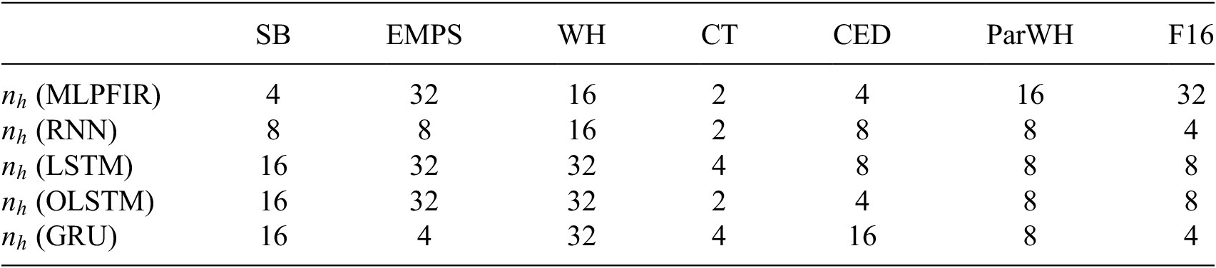
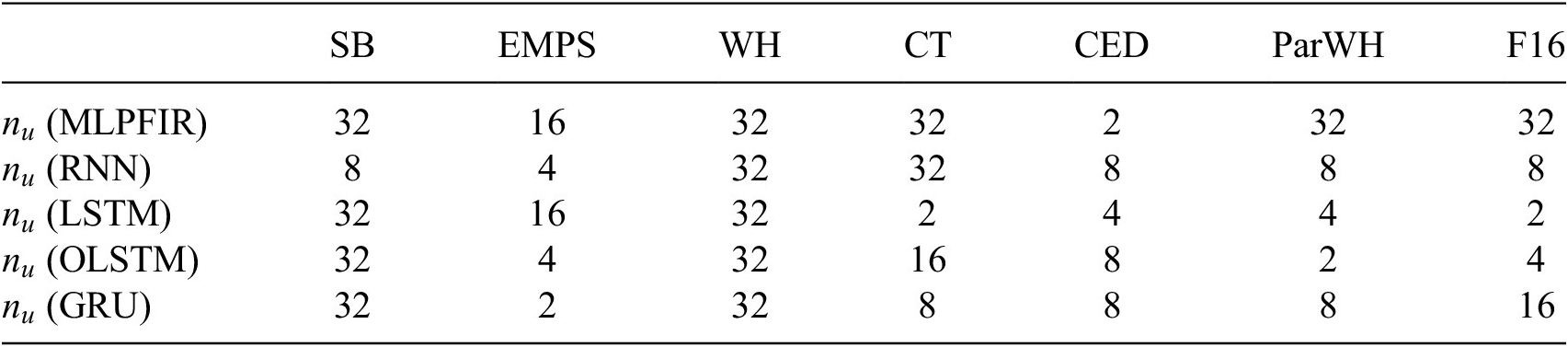
In all cases, the look-back distance and the dimension of the hidden memory state are selected by cross-validation on the hold-out validation set, with the best parameterization selected for evaluation on the testing set. The selected parameters are recorded here for the convenience of the reader in Tables 4 and 5. Training is conducted in batches, using 10 random initializations of the ADAM (with learning rate parameter
$ {10}^{-3} $
 ) optimizer for between
$ 2\times {10}^4 $
 and
$ {10}^4 $
 epochs depending on the amount of data available for training. Explicit descriptions of the various standard RNN architectures is well reported elsewhere and so is not reproduced here for reasons of space. The interested reader can see Goodfellow et al. (Reference Goodfellow, Bengio and Courville2016) for additional details on the models used in this study.
Number of RNN units (selected by cross-validation) used to generate baseline RNN results

Table 4. Long description
The table consists of 8 columns and 6 rows. The header row lists the datasets: S B, E M P S, W H, C T, C E D, Par W H, and F 16.
* Row 1: n sub h (M L P F I R) values are 4, 32, 16, 2, 4, 16, 32.
* Row 2: n sub h (R N N) values are 8, 8, 16, 2, 8, 8, 4.
* Row 3: n sub h (L S T M) values are 16, 32, 32, 4, 8, 8, 8.
* Row 4: n sub h (O L S T M) values are 16, 32, 32, 2, 4, 8, 8.
* Row 5: n sub h (G R U) values are 16, 4, 32, 4, 16, 8, 4.
Lookback distance
$ {n}_u $
 (selected by cross-validation) used to generate baseline RNN results

Table 5. Long description
The table consists of 8 columns and 6 rows.
Header Row: The columns are labeled from left to right as an empty cell, S B, E M P S, W H, C T, C E D, Par W H, and F 16.
Row 2: n sub u (M L P F I R) values are 32, 16, 32, 32, 2, 32, 32.
Row 3: n sub u (R N N) values are 8, 4, 32, 32, 8, 8, 8.
Row 4: n sub u (L S T M) values are 32, 16, 32, 2, 4, 4, 2.
Row 5: n sub u (O L S T M) values are 32, 4, 32, 16, 8, 2, 4.
Row 6: n sub u (G R U) values are 32, 2, 32, 8, 8, 8, 16.
4.3.1. MLP FIR
The first structure considered in this study is a (nonlinear) finite impulse response (FIR) model. This model structure is equivalent to removing the hidden ‘memory” state from the recurrence relation given earlier.

Where
$ F $
 is an MLP with a single hidden layer. The MLP FIR is essentially equivalent to the MLP NARX model with no lags on the output. Although this architecture is not recurrent, it will serve to highlight the extent to which a recurrent formulation improves the identification for each of the benchmark systems.
4.3.2. RNN
The canonical formulation of an RNN (Schuster and Paliwal, Reference Schuster and Paliwal1997) constructs the hidden cell as a single dense layer in an MLP, with a hyperbolic tangent activation function – other choices are clearly available. This architecture is employed here with the size of the hidden layer decided by cross-validation as described earlier.
4.3.3. GRU
A known issue with the RNN is that as the gradient is propagated backward in time, successive applications of the chain rule over activation functions can cause the numerical values of the gradients to become arbitrarily small or large. This issue is known as vanishing (resp. exploding) gradients (Pascanu et al., Reference Pascanu, Mikolov and Bengio2013). Several variants of the basic RNN cell have been proposed to try and combat this issue, by applying a “gating” function (often a sigmoid or similar) to the value of the memory state in each iteration. The gated recurrent network (GRU) (Chung et al., Reference Chung, Gulcehre, Cho and Bengio2014) is one such architecture that employs this technique.
4.3.4. LSTM
The original extension to the RNN is the famed long-short term memory (LSTM) unit (Hochreiter and Schmidhuber, Reference Hochreiter and Schmidhuber1997). This architecture propagates an extended hidden state consisting of both “long-term” and “short-term” memory. The optimised LSTM (OLSTM) is a variant of the LSTM cell that concatenates the hidden states prior to the activation functions for efficient computation. Results from both the LSTM and OLSTM networks are reported in this study.
5. Baseline results
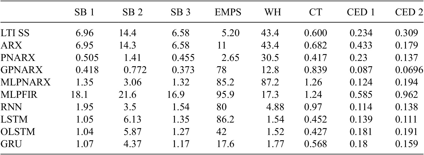
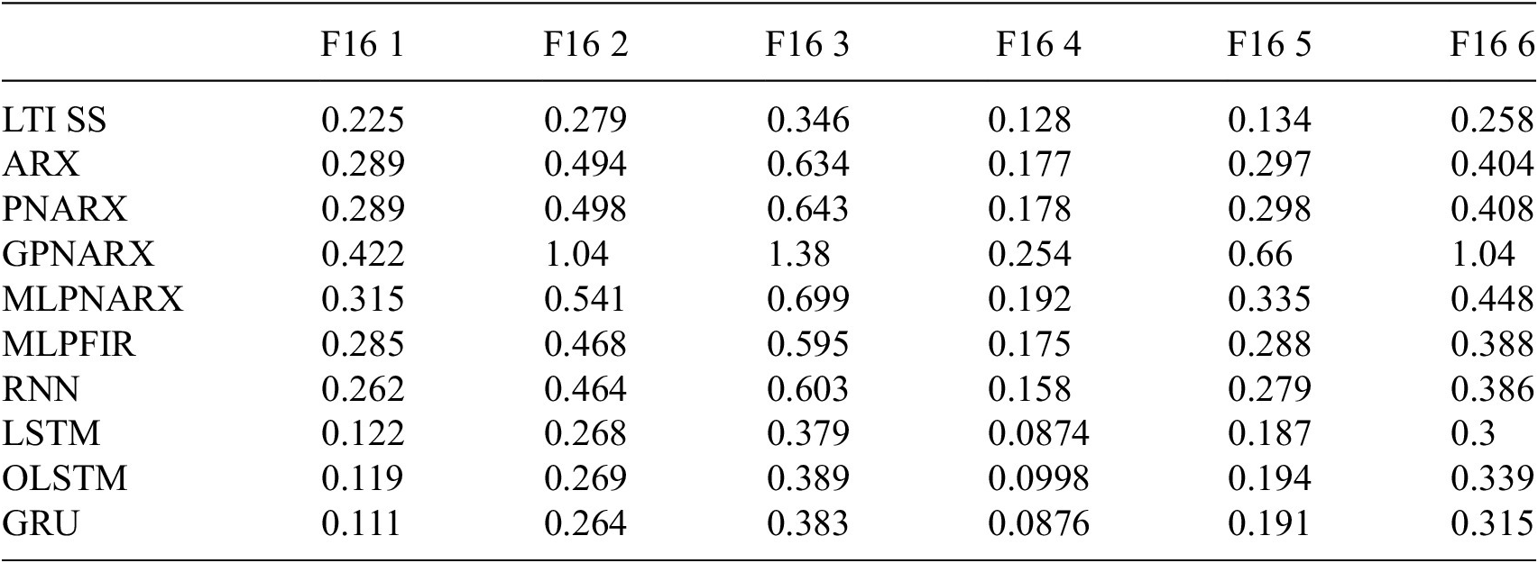
In order to establish the baseline results all of the models described earlier, they evaluated on the unseen testing set. For comparison, all model performances are reported using the RMSE metric in (3.1). These baseline results should help users of the benchmarks in positioning the outcome of their research. All model performances are reported in Tables 6–8 (Code to reproduce these baseline results can be found at https://github.com/MDCHAMP/nonlinear_baselines.). Note that in order to maintain readability, the reported error scores are not presented in the same units as the benchmarks. In particular, the SB, WH, ParWH, and EMPS benchmarks have been scaled by a factor of
$ {10}^3 $
 . To put these numbers in perspective, a selection of state-of-the-art (SOTA) results are collected for the benchmark datasets that have been studied in more detail in
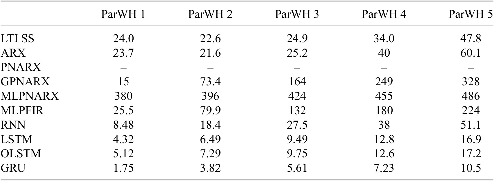
Table 9. During training, some baseline/benchmark combinations failed to produce a valid model. In particular, the PNARX model (fitted by least squares to the training data) produced unstable models (in simulation on the test data) at every model order on the ParWH benchmark.
Baseline results on the SB, EMPS, WH, CT, and CED benchmarks

Table 6. Long description
The table consists of nine columns. The first column lists the models, and the subsequent columns are S B 1, S B 2, S B 3, E M P S, W H, C T, C E D 1, and C E D 2.
* L T I S S: 6.96, 14.4, 6.58, 5.20, 43.4, 0.600, 0.234, 0.309.
* A R X: 6.95, 14.3, 6.58, 11, 43.4, 0.682, 0.433, 0.179.
* P N A R X: 0.505, 1.41, 0.455, 2.65, 30.5, 0.417, 0.23, 0.137.
* G P N A R X: 0.418, 0.772, 0.373, 78, 12.8, 0.839, 0.087, 0.0696.
* M L P N A R X: 1.35, 3.06, 1.32, 85.2, 87.2, 1.26, 0.124, 0.194.
* M L P F I R: 18.1, 21.6, 16.9, 95.9, 17.3, 1.24, 0.585, 0.962.
* R N N: 1.95, 3.5, 1.54, 80, 4.88, 0.97, 0.114, 0.138.
* L S T M: 1.05, 6.13, 1.35, 86.2, 1.54, 0.452, 0.139, 0.111.
* O L S T M: 1.04, 5.87, 1.27, 42, 1.52, 0.427, 0.181, 0.191.
* G R U: 1.07, 4.37, 1.17, 17.6, 1.77, 0.568, 0.18, 0.159.
Baseline results on the ParWH benchmark system

Table 7. Long description
The table consists of six columns. The first column lists the model types, and the subsequent five columns are headed ParWH 1, ParWH 2, ParWH 3, ParWH 4, and ParWH 5.
* L T I S S: 24.0, 22.6, 24.9, 34.0, 47.8.
* A R X: 23.7, 21.6, 25.2, 40, 60.1.
* P N A R X: No data provided for any system.
* G P N A R X: 15, 73.4, 164, 249, 328.
* M L P N A R X: 380, 396, 424, 455, 486.
* M L P F I R: 25.5, 79.9, 132, 180, 224.
* R N N: 8.48, 18.4, 27.5, 38, 51.1.
* L S T M: 4.32, 6.49, 9.49, 12.8, 16.9.
* O L S T M: 5.12, 7.29, 9.75, 12.6, 17.2.
* G R U: 1.75, 3.82, 5.61, 7.23, 10.5.
Baseline results on the F16 benchmark system

Table 8. Long description
The table consists of seven columns. The first column lists the model names, and the subsequent six columns are headed F 1 6 1 through F 1 6 6.
* L T I S S: 0.225, 0.279, 0.346, 0.128, 0.134, 0.258.
* A R X: 0.289, 0.494, 0.634, 0.177, 0.297, 0.404.
* P N A R X: 0.289, 0.498, 0.643, 0.178, 0.298, 0.408.
* G P N A R X: 0.422, 1.04, 1.38, 0.254, 0.66, 1.04.
* M L P N A R X: 0.315, 0.541, 0.699, 0.192, 0.335, 0.448.
* M L P F I R: 0.285, 0.468, 0.595, 0.175, 0.288, 0.388.
* R N N: 0.262, 0.464, 0.603, 0.158, 0.279, 0.386.
* L S T M: 0.122, 0.268, 0.379, 0.0874, 0.187, 0.3.
* O L S T M: 0.119, 0.269, 0.389, 0.0998, 0.194, 0.339.
* G R U: 0.111, 0.264, 0.383, 0.0876, 0.191, 0.315.
Selected state-of-the-art results available in the literature

Table 9. Long description
The table lists performance metrics for seven different models across several benchmarks. The columns are categorized by benchmark and unit: S B R M S in m V (Multisine, Arrow full, Arrow no extrap.), W H R M S in m V (Test), E M P S R M S in m m (Test), C T R M S in V (Test), and C E D R M S in ticks forward slash s (Test 1 and Test 2).
* D T subnet (Beintema et al., 2021): S B Multisine 0.36, Arrow full 1.4, Arrow no extrap. 0.32; W H 0.241; C T 0.37; C E D Test 1 0.169, Test 2 0.117.
* C T subnet (Beintema et al., 2023): E M P S 4.61; C T 0.306; C E D Test 1 0.115, Test 2 0.074.
* Grey-box (Worden et al., 2018): C T 0.191.
* P N L S S (Paduart et al., 2010, 2012; Relan et al., 2017): S B Arrow full 0.26; W H 0.42; C T 0.45.
* T S E M (Forgione and Piga, Reference Forgione and Piga2021a): C T 0.33.
* S C I (Forgione and Piga, Reference Forgione and Piga2021a): C T 0.4.
* dynoNet (Forgione and Piga, Reference Forgione and Piga2021b): W H 0.452; E M P S 2.64.
Overall, the performance of the different baseline approaches varies quite dramatically from benchmark to benchmark. In particular, for the performances on the SB, CED and CT approach the SOTA results for some baseline approaches. In particular, the pNARX, GP NARX, GRU, and LSTM models all offer very competitive results. This serves as an indication of the relative ease of modeling these systems in the black-box setting.
In contrast, the baseline performances on the WH and EMPS systems lag significantly behind SOTA scores. Despite a qualitatively good fit to the data, the baseline results on the WH benchmark remain an order of magnitude away from the SOTA results. A possible explanation for this is the saturation nonlinearity inside the WH block structure. This type of nonlinearity is particularly difficult for black-box learners, despite the linear-dominated dynamics of the WH system. The presence of a friction nonlinearity in the EMPS benchmark is particularly challenging for linear models to approximate.
On a third subset of benchmark problems (ParWH, F16), neither baseline methods nor SOTA methods produce good models (particularly at large excitation levels), an indication that these systems offer a more robust identification challenge. Only dedicated ParWH methods have reported results that approach the noise floor (Schoukens et al., Reference Schoukens, Marconato, Pintelon, Vandersteen and Rolain2015). Indeed, large data lengths, higher model orders, and possibly harsh nonlinearities (F16) make these systems difficult for black-box learners.
It is unsurprising that in almost every case, the ARX and LTI SS models achieve very similar scores on the benchmark problems although the LTI ARX model typically requires a higher model order to correctly capture the disturbances present in the data. For some of the longest test sets (such as those in the F16 and ParWH systems), these performances diverge at larger excitation levels, possibly indicating that the LTI SS models are better generalized than ARX. This could be due to the simulation error focus of the specific LTI SS identification algorithm used here, compared to the 1-step ahead prediction focus of ARX.
A noteworthy observation is that for the EMPS, CT and F16 benchmarks, none of the nonlinear baselines significantly outperforms the LTI SS or ARX baselines. However, as mentioned earlier, better results have been reported in the literature (see e.g. Table 9).
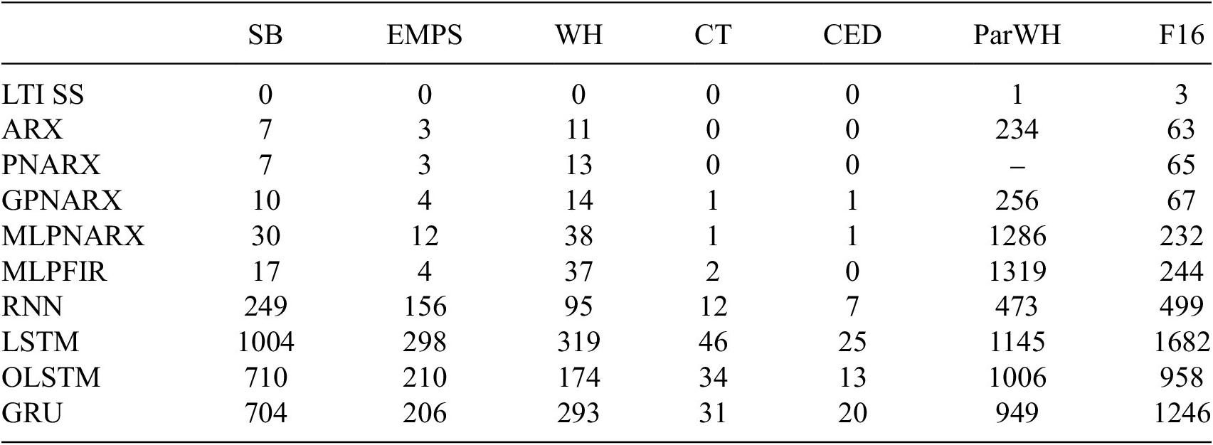
One interesting outcome from the baseline results is the performance of the PNARX model. In all benchmarks, the polynomial model demonstrates robust performances (close to or up to a factor 2 worse than SOTA for SB, EMPS, CT and CED). Especially remarkable is that these results can be achieved for very little computational effort, even in the presence of large training sequences, and considering only monomial terms (that is no cross-terms) in the model (Billings, Reference Billings2013). The training time reported in 9 is actually dominated in most cases by the ARX lag structure optimization with the actual training of PNARX models taking only a few seconds. This motivates the use of PNARX as a “first analysis” in the black-box NLSI setting.
Finally, it can be observed that the total time taken by each method to complete the training, cross-validation, and prediction varies strongly (see Table 10): the computationally more simple approaches take a couple of minutes or less, while some of the RNN-based approaches take multiple hours. This is in part due to the increased number of model structure decision variables that need to be tuned (number of input/output lags, number of states, number of neurons and hidden layers), but also due to the larger number of parameters and the different types of optimization approaches that are being used (e.g., ordinary least squares, Gauss-Newton, or gradient based methods) This can become an important consideration when models need to be trained on lightweight processors, or within a limited time window.
Total time taken in training, cross-validation, and prediction of the baseline methods considered in this study, rounded to the nearest whole minute

Table 10. Long description
The table consists of 8 columns and 11 rows. The columns are labeled from left to right as: Method, S B, E M P S, W H, C T, C E D, Par W H, and F 16.
* L T I S S: 0, 0, 0, 0, 0, 1, 3.
* A R X: 7, 3, 11, 0, 0, 234, 63.
* P N A R X: 7, 3, 13, 0, 0, dash, 65.
* G P N A R X: 10, 4, 14, 1, 1, 256, 67.
* M L P N A R X: 30, 12, 38, 1, 1, 1286, 232.
* M L P F I R: 17, 4, 37, 2, 0, 1319, 244.
* R N N: 249, 156, 95, 12, 7, 473, 499.
* L S T M: 1004, 298, 319, 46, 25, 1145, 1682.
* O L S T M: 710, 210, 174, 34, 13, 1006, 958.
* G R U: 704, 206, 293, 31, 20, 949, 1246.
6. Conclusion
The present paper reflected on a number of key aspects of what constitutes a good system identification benchmark. Next, this reflection is translated into practice through the nonlinearbenchmark.org platform. The website hosts a number of accessible datasets, including a detailed description and a number of baseline results, that are reported on a leaderboard. The data is easy to access through dedicated data loader scripts, and new results can be submitted through a webform. The baseline results indicated that some datasets such as the Silverbox and Cascaced Tanks benchmarks offer a good entry- to medium-level challenges, while others such as the ParWH and F16 data prove to be more challenging.
Data availability statement
All benchmark datasets are available through https://www.nonlinearbenchmark.org/ (Schoukens and Noël, Reference Schoukens and Noël2026). The archived code of the corresponding GitHub repositories are available on Zenodo: (Beintema et al., Reference Beintema, Schoukens, Busetto, Retzler, Champneys and Floren2026; Champneys, 2026).
Acknowledgments
The authors thank J.P. Noël, a founding member of the nonlinearbenchmark.org platform and coauthor of many of the featured datasets, and K. Tiels for their support in building the nonlinearbenchmark.org community through the annual workshop and minicourse. We also thank all the researchers who have contributed to the development of the datasets featured on the nonlinearbenchmark.org website.
M.D. Champneys gratefully acknowledges the support of the Centre for Machine Intelligence (CMI) within the University of Sheffield.
Author contribution
Conceptualization: M.S., M.D.C., G.I.B., T.J.R.; Data Curation: M.S.; Methodology: M.S., M.D.C., G.I.B., T.J.R.; Software: M.D.C., G.I.B., M.S.; Supervision: M.S., T.J.R.; Writing—Original Draft: M.S., M.D.C., G.I.B.; Writing—Review and Editing: M.S., M.D.C., G.I.B., T.J.R.
Funding statement
M. Schoukens and G.I. Beintema were funded by the European Union (ERC, COMPLETE, 101075836). Views and opinions expressed are, however, those of the author(s) only and do not necessarily reflect those of the European Union or the European Research Council Executive Agency. Neither the European Union nor the granting authority can be held responsible for them.
M.D. Champneys and T. Rogers were supported by the EPSRC grant EP/W002140/1.
M.D. Champneys and T. Rogers gratefully acknowledge the support of the UK Engineering and Physical Sciences Research Council (EPSRC) via grant references EP/W005816/1 and EP/W002140/1.
Open access funding provided by Eindhoven University of Technology.
Competing interests
The authors declare none.
Ethical standard
The research meets all ethical guidelines, including adherence to the legal requirements of the study country.








 Open access


Comments
No Comments have been published for this article.