1 Introduction
Diffusion-driven flow occurs when a quiescent stably stratified viscous fluid is in contact with an inclined insulated surface (for temperature stratification) or impermeable surface (for salt stratification). This flow was examined independently by Phillips (Reference Phillips1970) and Wunsch (Reference Wunsch1970) for sloping planar surfaces in which horizontal lines of constant density bend to meet the surface at right angles. As a result, hydrostatic pressure equilibrium is disturbed and slow fluid motion is induced along the sloping surface, balanced by viscous drag. Phillips (Reference Phillips1970) examined the importance of these flows to mass transport along a fissure in a geological context while Wunsch (Reference Wunsch1970) postulated that the boundary layers arising from the motion might play a role in oceanic mixing. More recently, Dell & Pratt (Reference Dell and Pratt2015) suggested that it could drive upwelling near mid-ocean ridges.
Diffusion-driven flow has also been studied on other geometrical objects with sloping surfaces, for example, a finite-length plate (Woods Reference Woods1991; Zagumennyi & Chashechkin Reference Zagumennyi and Chashechkin2013a ,Reference Zagumennyi and Chashechkin b ,Reference Zagumennyi and Chashechkin c ), a wedge (Allshouse, Barad & Peacock Reference Allshouse, Barad and Peacock2010; Zagumennyi & Chashechkin Reference Zagumennyi and Chashechkin2013c ) and a sphere (Baidulov, Matyushin & Chashechkin Reference Baidulov, Matyushin and Chashechkin2005, Reference Baidulov, Matyushin and Chashechkin2007). Internal flows have been considered for a tilted square container (Quon Reference Quon1976, Reference Quon1983; Page & Johnson Reference Page and Johnson2008, Reference Page and Johnson2009; Page Reference Page2011a ,Reference Page b ) and inside a cylinder (Quon Reference Quon1989; Page & Johnson Reference Page and Johnson2009), as prototypes to illustrate some of the key dynamical features that can arise more generally. Allshouse et al. (Reference Allshouse, Barad and Peacock2010), in particular, showed the induced flow can propel a wedge-shaped object, albeit slowly. All of these studies considered the case where the boundary-layer thickness is small relative to the size of the object.
In contrast, this paper investigates the analytical properties of steady two-dimensional diffusion-driven flow around a small axisymmetrical object in the situation where the thickness of the layer is very large in comparison to its size. As a prototype for this regime, the streamfunction and density fields of a linearly stratified fluid around a fixed, infinite-length horizontal cylinder are derived analytically based on perturbation theory when the Reynolds number based on the induced velocity is very small. The choice of a circular cylinder is for analytical convenience, as many of the qualitative results can be expected to apply for other geometrical shapes, including three-dimensional objects.
The key parameter here is
 $\unicode[STIX]{x1D716}=(N^{\ast }L^{\ast 2}/\unicode[STIX]{x1D708}^{\ast })^{2}$
, where
 $N^{\ast }$
is a buoyancy frequency,
 $L^{\ast }$
is a typical object size and
 $\unicode[STIX]{x1D708}^{\ast }$
is a kinematic viscosity. It is assumed that
 $\unicode[STIX]{x1D716}\ll 1$
and that the Prandtl number
 $\unicode[STIX]{x1D70E}=\unicode[STIX]{x1D708}^{\ast }/\unicode[STIX]{x1D705}^{\ast }$
is of order one with respect to that parameter, where
 $\unicode[STIX]{x1D705}^{\ast }$
is the density diffusivity. In contrast, Wunsch (Reference Wunsch1970) assumed that
 ${\mathcal{R}}=\sqrt{\unicode[STIX]{x1D708}^{\ast }\unicode[STIX]{x1D705}^{\ast }}/(N^{\ast }L^{\ast 2})$
was small, which corresponds to
 $\unicode[STIX]{x1D716}\gg 1$
here, and he deduced that the boundary-layer thickness was
 $O({\mathcal{R}}^{1/2})$
. Here it is shown that
 $\unicode[STIX]{x1D716}$
is effectively the Reynolds number based on the deduced speed
 $U^{\ast }=N^{\ast 2}L^{\ast 3}/\unicode[STIX]{x1D708}^{\ast }$
of the induced flow, and so
 $\unicode[STIX]{x1D716}\ll 1$
corresponds to the low-Reynolds-number case, for which in a homogeneous fluid the viscous interactions between particles can extend over large distances (Tritton Reference Tritton1988, p. 99). One reason for considering this regime is to examine the diffusion-driven flow induced by very small particles in a stratified fluid, for example in the ocean. The
 $\unicode[STIX]{x1D70E}=O(1)$
assumption is reasonable for temperature stratification but, for the leading order at least, the theory here is expected to remain representative across a broad range of
 $\unicode[STIX]{x1D70E}$
values when
 $\unicode[STIX]{x1D716}$
is very small, including arguably in salt-stratified water where
 $\unicode[STIX]{x1D70E}\sim 10^{3}$
is more typical.
Analytical solutions for streamfunction and density are derived using a two-region approach in an analogous manner to how Oseen flow in a homogeneous fluid assists in the resolution of Stokes’ paradox (Van Dyke Reference Van Dyke1975). This is necessary because the solutions for the velocity and density perturbation over the length scale of the object do not vanish at large radius, whereas the far-field fluid is assumed unaffected by the presence of the cylinder. The ‘inner region’ is on a similar length scale to the object, but the ‘outer region’ extends over a larger length scale, which turns out to be
 $O(L^{\ast }(\unicode[STIX]{x1D70E}\unicode[STIX]{x1D716})^{-1/4})$
or
 $(\unicode[STIX]{x1D705}^{\ast }\unicode[STIX]{x1D708}^{\ast }/N^{\ast 2})^{1/4}$
in terms of the dimensional quantities above. A similar type of approach was used by both Zvirin & Chadwick (Reference Zvirin and Chadwick1975) and Candelier, Mehaddi & Vauquelin (Reference Candelier, Mehaddi and Vauquelin2014) to examine motion due to a falling sphere in a viscous stratified fluid, although there are differences in detail due to the different geometry and parameter regime.
The flow configuration and equations of motion are presented in § 2, leading to the analytical inner solutions in § 3. Outer solutions are derived and presented in § 4 in terms of Fourier transforms, and then evaluated numerically from their integral expressions. Asymptotic solutions at the inner edge of the outer region are derived analytically and matched to those in the inner region. Asymptotic solutions at the outer edge of the outer layer are also derived by analytical methods and are compared with similar features in previous studies. Results show that the outer solutions for the streamfunction and the density exist and match both the inner and far-field solutions at leading order.
2 Governing equations
A horizontal cylinder of radius
 $a^{\ast }$
is immersed in a continuously stratified viscous fluid with density that decreases linearly with height. Cartesian coordinates
 $\boldsymbol{x}^{\ast }=(x^{\ast },y^{\ast },z^{\ast })$
are defined with
 $x^{\ast }$
and
 $y^{\ast }$
parallel to planes of constant density, the
 $y^{\ast }$
-axis aligned with the cylinder axis and
 $z^{\ast }$
directed opposite to the gravitational acceleration
 $g^{\ast }$
. The fluid is assumed incompressible, with small density variations allowed. The undisturbed ‘background’ density is taken to have a linear profile
 $\unicode[STIX]{x1D70C}_{b}^{\ast }=\unicode[STIX]{x1D70C}_{00}^{\ast }-\unicode[STIX]{x1D70C}_{0}^{\prime \ast }z^{\ast }$
in dimensional form, where
 $\unicode[STIX]{x1D70C}_{00}^{\ast }$
is a reference value and
 $\unicode[STIX]{x1D70C}_{0}^{\prime \ast }>0$
. In the absence of fluid motion, the ‘background’ pressure
 $P_{b}^{\ast }=P_{00}^{\ast }-g^{\ast }\unicode[STIX]{x1D70C}_{00}^{\ast }z^{\ast }+\unicode[STIX]{x1D70C}_{0}^{\prime \ast }z^{\ast 2}/2$
satisfies hydrostatic equilibrium
 $\unicode[STIX]{x1D735}^{\ast }P_{b}^{\ast }=-g^{\ast }\unicode[STIX]{x1D70C}_{b}^{\ast }\hat{\boldsymbol{k}}$
, where
 $P_{00}^{\ast }$
is a constant,
 $\unicode[STIX]{x1D735}^{\ast }=(\unicode[STIX]{x2202}/\unicode[STIX]{x2202}x^{\ast },\unicode[STIX]{x2202}/\unicode[STIX]{x2202}y^{\ast },\unicode[STIX]{x2202}/\unicode[STIX]{x2202}z^{\ast })$
and
 $\hat{\boldsymbol{k}}$
is a unit vector in the
 $z^{\ast }$
-direction.
The velocity of the slow induced motion
 $\boldsymbol{u}^{\ast }=(u^{\ast },v^{\ast },w^{\ast })$
is assumed steady and two-dimensional, with
 $v^{\ast }=0$
everywhere. Based on the geometry, all quantities are taken to be independent of
 $y^{\ast }$
.
Non-dimensional coordinates are defined here with
 $\boldsymbol{x}=(x,z)=\boldsymbol{x}^{\ast }/a^{\ast }$
, using the scaled density
 $\unicode[STIX]{x1D70C}=(\unicode[STIX]{x1D70C}^{\ast }-\unicode[STIX]{x1D70C}_{00}^{\ast })/a^{\ast }\unicode[STIX]{x1D70C}_{0}^{\prime \ast }$
and pressure
 $P=(P^{\ast }-P_{00}^{\ast }+g^{\ast }\unicode[STIX]{x1D70C}_{00}^{\ast }z^{\ast })/g^{\ast }a^{\ast 2}\unicode[STIX]{x1D70C}_{0}^{\prime \ast }$
. In terms of a reference velocity
 $U^{\ast }$
identified below, the induced non-dimensional velocity is
 $\boldsymbol{u}=(u,w)=\boldsymbol{u}^{\ast }/U^{\ast }$
.
The Navier–Stokes equation for steady two-dimensional flow under the Boussinesq approximation is, in non-dimensional form,
 $$\begin{eqnarray}\unicode[STIX]{x1D716}(\boldsymbol{u}\boldsymbol{\cdot }\unicode[STIX]{x1D735})\boldsymbol{u}=-\unicode[STIX]{x1D735}P-\unicode[STIX]{x1D70C}\hat{\boldsymbol{k}}+\unicode[STIX]{x1D6FB}^{2}\boldsymbol{u}.\end{eqnarray}$$
It is assumed here, and demonstrated below, that the non-hydrostatic pressure variations of magnitude one due to the cylinder give rise to a diffusion-driven flow with speed of magnitude
 $U^{\ast }=N^{\ast 2}a^{\ast 3}/\unicode[STIX]{x1D708}^{\ast }$
, in terms of the buoyancy frequency
 $N^{\ast }=\sqrt{g^{\ast }\unicode[STIX]{x1D70C}_{0}^{\prime \ast }/\unicode[STIX]{x1D70C}_{00}^{\ast }}$
. The parameter
 $\unicode[STIX]{x1D716}$
in (2.1), given by
 $$\begin{eqnarray}\unicode[STIX]{x1D716}=N^{\ast 2}a^{\ast 4}/\unicode[STIX]{x1D708}^{\ast 2}=U^{\ast }a^{\ast }/\unicode[STIX]{x1D708}^{\ast },\end{eqnarray}$$
is therefore a relevant Reynolds number. Correspondingly, density variations satisfy
 $$\begin{eqnarray}\unicode[STIX]{x1D70E}\unicode[STIX]{x1D716}(\boldsymbol{u}\boldsymbol{\cdot }\unicode[STIX]{x1D735})\unicode[STIX]{x1D70C}=\unicode[STIX]{x1D6FB}^{2}\unicode[STIX]{x1D70C},\end{eqnarray}$$
where
 $\unicode[STIX]{x1D70E}$
is the Prandtl number, with
 $\unicode[STIX]{x1D735}\boldsymbol{\cdot }\boldsymbol{u}=0$
for an incompressible fluid. These equations have similar forms to those in Wunsch (Reference Wunsch1970), but with some differences due to the scaling factors. As noted in § 1, it is assumed here that
 $\unicode[STIX]{x1D716}\ll 1$
. Although
 $\unicode[STIX]{x1D70E}$
can be large in some cases (for example in salt-stratified water), for the purposes of the asymptotic theory here
 $\unicode[STIX]{x1D70E}$
is treated as
 $O(1)$
with respect to
 $\unicode[STIX]{x1D716}$
.
As the object is circular here, polar coordinates
 $(r,\unicode[STIX]{x1D703})$
are introduced with
 $x=r\sin \unicode[STIX]{x1D703}$
and
 $z=r\cos \unicode[STIX]{x1D703}$
, so that
 $r=\sqrt{x^{2}+z^{2}}$
and
 $\unicode[STIX]{x1D703}=\arctan (x/z)$
is directed clockwise from the
 $z$
axis towards the
 $x$
axis for right-handedness. A streamfunction
 $\unicode[STIX]{x1D713}(r,\unicode[STIX]{x1D703})$
is introduced in terms of which the induced velocity
 $\boldsymbol{u}=(u_{r},u_{\unicode[STIX]{x1D703}})$
is given by
 $$\begin{eqnarray}u_{r}=\frac{1}{r}\frac{\unicode[STIX]{x2202}\unicode[STIX]{x1D713}}{\unicode[STIX]{x2202}\unicode[STIX]{x1D703}}\quad \text{and}\quad u_{\unicode[STIX]{x1D703}}=-\frac{\unicode[STIX]{x2202}\unicode[STIX]{x1D713}}{\unicode[STIX]{x2202}r}.\end{eqnarray}$$
In terms of these coordinates, after eliminating the pressure from the
 $x$
and
 $z$
components of (2.1), it follows that
 $$\begin{eqnarray}\unicode[STIX]{x1D6FB}^{4}\unicode[STIX]{x1D713}=\left(\sin \unicode[STIX]{x1D703}\frac{\unicode[STIX]{x2202}\unicode[STIX]{x1D70C}}{\unicode[STIX]{x2202}r}+\frac{\cos \unicode[STIX]{x1D703}}{r}\frac{\unicode[STIX]{x2202}\unicode[STIX]{x1D70C}}{\unicode[STIX]{x2202}\unicode[STIX]{x1D703}}\right)+\frac{\unicode[STIX]{x1D716}}{r}\left(\frac{\unicode[STIX]{x2202}\unicode[STIX]{x1D713}}{\unicode[STIX]{x2202}\unicode[STIX]{x1D703}}\frac{\unicode[STIX]{x2202}}{\unicode[STIX]{x2202}r}-\frac{\unicode[STIX]{x2202}\unicode[STIX]{x1D713}}{\unicode[STIX]{x2202}r}\frac{\unicode[STIX]{x2202}}{\unicode[STIX]{x2202}\unicode[STIX]{x1D703}}\right)\unicode[STIX]{x1D6FB}^{2}\unicode[STIX]{x1D713},\end{eqnarray}$$
where
 $\unicode[STIX]{x1D6FB}^{2}$
is the two-dimensional Laplacian in polar coordinates, and also (2.3) becomes
 $$\begin{eqnarray}\unicode[STIX]{x1D6FB}^{2}\unicode[STIX]{x1D70C}=\frac{\unicode[STIX]{x1D70E}\unicode[STIX]{x1D716}}{r}\left(\frac{\unicode[STIX]{x2202}\unicode[STIX]{x1D713}}{\unicode[STIX]{x2202}\unicode[STIX]{x1D703}}\frac{\unicode[STIX]{x2202}\unicode[STIX]{x1D70C}}{\unicode[STIX]{x2202}r}-\frac{\unicode[STIX]{x2202}\unicode[STIX]{x1D713}}{\unicode[STIX]{x2202}r}\frac{\unicode[STIX]{x2202}\unicode[STIX]{x1D70C}}{\unicode[STIX]{x2202}\unicode[STIX]{x1D703}}\right).\end{eqnarray}$$
The streamfunction must satisfy
 $\unicode[STIX]{x2202}\unicode[STIX]{x1D713}/\unicode[STIX]{x2202}r=0$
at
 $r=1$
from the no-slip condition on the cylinder surface and, without loss of generality,
 $\unicode[STIX]{x1D713}=0$
at
 $r=1$
. The fluid is assumed to be stationary in the far field, so the streamfunction is bounded. An insulating condition is imposed on the density at the cylinder surface, with
 $\unicode[STIX]{x2202}\unicode[STIX]{x1D70C}/\unicode[STIX]{x2202}r=0$
at
 $r=1$
. Far from the cylinder, the density of the stratified fluid is assumed to match the scaled linear ‘background’ value
 $\unicode[STIX]{x1D70C}_{b}=-z=-r\cos \unicode[STIX]{x1D703}$
, with
 $\unicode[STIX]{x1D70C}\rightarrow \unicode[STIX]{x1D70C}_{b}$
as
 $r\rightarrow \infty$
.
In § 3 it is found that solutions
 $\unicode[STIX]{x1D713}$
and
 $\unicode[STIX]{x1D70C}$
of (2.5) and (2.6) when
 $\unicode[STIX]{x1D716}=0$
violate the conditions for the far-field flow. In § 4 an ‘outer’ region is introduced to resolve this problem, analogous to how Oseen’s method overcomes similar issues at large radius for flow past a cylinder in a homogeneous viscous fluid, see Van Dyke (Reference Van Dyke1975) for example.
3 Inner region
 $r=O(1)$

For
 $\unicode[STIX]{x1D716}\ll 1$
, the streamfunction and density near the cylinder are assumed of the form
 $$\begin{eqnarray}\unicode[STIX]{x1D713}(r,\unicode[STIX]{x1D703})=\unicode[STIX]{x1D713}_{0}(r,\unicode[STIX]{x1D703})+\unicode[STIX]{x1D716}\unicode[STIX]{x1D713}_{1}(r,\unicode[STIX]{x1D703})+\cdots \quad \text{and}\quad \unicode[STIX]{x1D70C}(r,\unicode[STIX]{x1D703})=\unicode[STIX]{x1D70C}_{0}(r,\unicode[STIX]{x1D703})+\unicode[STIX]{x1D716}\unicode[STIX]{x1D70C}_{1}(r,\unicode[STIX]{x1D703})+\cdots \,,\end{eqnarray}$$
for which the first-order and second-order terms are derived below. Each term may include logarithmic terms in
 $\unicode[STIX]{x1D716}$
, but for simplicity these are grouped by integer powers of
 $\unicode[STIX]{x1D716}$
. Substituting (3.1) into (2.5) and (2.6) gives
 $$\begin{eqnarray}\unicode[STIX]{x1D6FB}^{4}\unicode[STIX]{x1D713}_{0}=\left(\sin \unicode[STIX]{x1D703}\frac{\unicode[STIX]{x2202}\unicode[STIX]{x1D70C}_{0}}{\unicode[STIX]{x2202}r}+\frac{\cos \unicode[STIX]{x1D703}}{r}\frac{\unicode[STIX]{x2202}\unicode[STIX]{x1D70C}_{0}}{\unicode[STIX]{x2202}\unicode[STIX]{x1D703}}\right)\quad \text{and}\quad \unicode[STIX]{x1D6FB}^{2}\unicode[STIX]{x1D70C}_{0}=0.\end{eqnarray}$$
Assuming
 $\unicode[STIX]{x1D70C}_{0}(r,\unicode[STIX]{x1D703})=G_{01}(r)\cos \unicode[STIX]{x1D703}$
based on the symmetry of far-field density, and requiring
 $\unicode[STIX]{x2202}\unicode[STIX]{x1D70C}_{0}/\unicode[STIX]{x2202}r=0$
at
 $r=1$
and
 $\unicode[STIX]{x1D70C}_{0}\rightarrow -r\cos \unicode[STIX]{x1D703}$
as
 $r\rightarrow \infty$
yields
 $$\begin{eqnarray}\unicode[STIX]{x1D70C}_{0}(r,\unicode[STIX]{x1D703})=-(r+1/r)\cos \unicode[STIX]{x1D703}.\end{eqnarray}$$
The
 $\cos \unicode[STIX]{x1D703}/r$
term in (3.3) breaks the hydrostatic equilibrium of a stationary fluid, and is associated with a horizontal pressure gradient. As observed for other ‘diffusion-driven’ flows, see for example Page & Johnson (Reference Page and Johnson2009), this pressure difference induces slow ‘upslope’ motion aligned with the upper cylinder surface (and ‘downslope’ near the lower surface) which is steady when the buoyancy is balanced by the viscous forces.
Substituting (3.3) into (3.2a
) suggests a solution of the form
 $\unicode[STIX]{x1D713}_{0}(r,\unicode[STIX]{x1D703})=F_{02}(r)\sin 2\unicode[STIX]{x1D703}$
(where the second subscript refers to
 $n\unicode[STIX]{x1D703}$
hereinafter) and requiring
 $\unicode[STIX]{x1D713}_{0}=\unicode[STIX]{x2202}\unicode[STIX]{x1D713}_{0}/\unicode[STIX]{x2202}r=0$
at
 $r=1$
gives
 $$\begin{eqnarray}\unicode[STIX]{x1D713}_{0}(r,\unicode[STIX]{x1D703})=\bigg[c_{0}\bigg(\frac{1}{r^{2}}-2+r^{2}\bigg)-\frac{1}{2r^{2}}+\frac{1}{2}-r^{2}\ln r\bigg]\frac{\sin 2\unicode[STIX]{x1D703}}{16},\end{eqnarray}$$
where
 $c_{0}$
is an as yet undetermined constant. A possible
 $O(r^{4})$
term is omitted from (3.4), based on the far-field assumptions, while at least some
 $O(r^{2})$
terms must be present due to the forcing. When
 $c_{0}>{\textstyle \frac{3}{4}}$
the motion adjacent to the cylinder follows the typical direction for diffusion-driven flow, ascending for
 $z>0$
and with descending flow for
 $z<0$
. In this case
 $\unicode[STIX]{x1D713}_{0}$
always changes sign at some radius
 $r_{0}>1$
, reversing the far-field flow direction, with
 $r_{0}\approx \exp (c_{0})$
when
 $r_{0}$
is large. It will be seen below that
 $c_{0}$
is determined from matching onto the outer region, with a large positive value that turns out to be
 $O(\unicode[STIX]{x1D716}^{-1/4})$
when
 $\unicode[STIX]{x1D716}\ll 1$
(and so the
 $c_{0}\leqslant {\textstyle \frac{3}{4}}$
case is not pursued here).
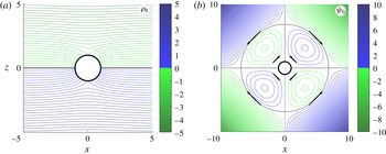
Lines of constant (a) density
 $\unicode[STIX]{x1D70C}_{0}(r,\unicode[STIX]{x1D703})$
for
 $-5\leqslant \{x,z\}\leqslant 5$
and (b) streamfunction
 $\unicode[STIX]{x1D713}_{0}(r,\unicode[STIX]{x1D703})$
when
 $c_{0}=2$
for
 $-10\leqslant \{x,z\}\leqslant 10$
based on the leading-order solutions in the inner region. The contour intervals used are 0.2 and 0.1, respectively.

Figure 1(a) illustrates the density field based on (3.3). The deflection of isopycnals near the cylinder is evident, so they meet the surface at right angles and satisfy
 $\unicode[STIX]{x2202}\unicode[STIX]{x1D70C}_{0}/\unicode[STIX]{x2202}r=0$
at
 $r=1$
. Figure 1(b) shows the streamlines of the induced flow based on the solution (3.4) for
 $c_{0}=2$
. The fluid close to the cylinder when
 $z>0$
ascends because its density is lighter than the far-field density at the same level, with the opposite happening for
 $z<0$
. As noted above,
 $\unicode[STIX]{x1D713}_{0}$
changes sign further away from the cylinder, at
 $r_{0}\approx 5.55$
when
 $c_{0}=2$
, and the flow moves in the opposite direction for large
 $r$
.
3.1 Second-order terms
From (2.5) and (2.6) the second-order terms
 $\unicode[STIX]{x1D713}_{1}$
and
 $\unicode[STIX]{x1D70C}_{1}$
satisfy
 $$\begin{eqnarray}\unicode[STIX]{x1D6FB}^{4}\unicode[STIX]{x1D713}_{1}=\left(\sin \unicode[STIX]{x1D703}\frac{\unicode[STIX]{x2202}\unicode[STIX]{x1D70C}_{1}}{\unicode[STIX]{x2202}r}+\frac{\cos \unicode[STIX]{x1D703}}{r}\frac{\unicode[STIX]{x2202}\unicode[STIX]{x1D70C}_{1}}{\unicode[STIX]{x2202}\unicode[STIX]{x1D703}}\right)+\frac{1}{r}\left(\frac{\unicode[STIX]{x2202}\unicode[STIX]{x1D713}_{0}}{\unicode[STIX]{x2202}\unicode[STIX]{x1D703}}\frac{\unicode[STIX]{x2202}}{\unicode[STIX]{x2202}r}-\frac{\unicode[STIX]{x2202}\unicode[STIX]{x1D713}_{0}}{\unicode[STIX]{x2202}r}\frac{\unicode[STIX]{x2202}}{\unicode[STIX]{x2202}\unicode[STIX]{x1D703}}\right)\unicode[STIX]{x1D6FB}^{2}\unicode[STIX]{x1D713}_{0}\end{eqnarray}$$
and
 $$\begin{eqnarray}\unicode[STIX]{x1D6FB}^{2}\unicode[STIX]{x1D70C}_{1}=\frac{\unicode[STIX]{x1D70E}}{r}\left(\frac{\unicode[STIX]{x2202}\unicode[STIX]{x1D713}_{0}}{\unicode[STIX]{x2202}\unicode[STIX]{x1D703}}\frac{\unicode[STIX]{x2202}\unicode[STIX]{x1D70C}_{0}}{\unicode[STIX]{x2202}r}-\frac{\unicode[STIX]{x2202}\unicode[STIX]{x1D713}_{0}}{\unicode[STIX]{x2202}r}\frac{\unicode[STIX]{x2202}\unicode[STIX]{x1D70C}_{0}}{\unicode[STIX]{x2202}\unicode[STIX]{x1D703}}\right),\end{eqnarray}$$
with
 $\unicode[STIX]{x2202}\unicode[STIX]{x1D70C}_{1}/\unicode[STIX]{x2202}r=0$
and
 $\unicode[STIX]{x1D713}_{1}=\unicode[STIX]{x2202}\unicode[STIX]{x1D713}_{1}/\unicode[STIX]{x2202}r=0$
at
 $r=1$
. Substituting (3.4) and (3.3) into the right-hand side of (3.6), assuming
 $\unicode[STIX]{x1D70C}_{1}(r,\unicode[STIX]{x1D703})=G_{11}(r)\cos \unicode[STIX]{x1D703}+G_{13}(r)\cos 3\unicode[STIX]{x1D703}$
, leads to
 $$\begin{eqnarray}\displaystyle \unicode[STIX]{x1D70C}_{1}(r,\unicode[STIX]{x1D703}) & = & \displaystyle \unicode[STIX]{x1D70E}\bigg[c_{0}\bigg(\frac{1}{r^{3}}+\frac{2}{r}-r^{3}+\frac{4(1+r^{2})}{r}\ln r\bigg)-\frac{1}{2r^{3}}-\frac{r^{3}}{2}-\frac{(1-r^{4})}{r}\ln r\bigg]\frac{\cos \unicode[STIX]{x1D703}}{64}\nonumber\\ \displaystyle & & \displaystyle +\,\unicode[STIX]{x1D70E}\bigg[d_{1}\bigg(\frac{1}{r^{3}}+r^{3}\bigg)-c_{0}\bigg(\frac{4}{r^{3}}-\frac{6}{r}+6r\bigg)\nonumber\\ \displaystyle & & \displaystyle +\,\frac{13}{6r^{3}}-\frac{9}{4r}+\frac{9r}{4}+(3r-r^{3})\ln r\bigg]\frac{\cos 3\unicode[STIX]{x1D703}}{192},\end{eqnarray}$$
where
 $d_{1}$
is an undetermined constant and the
 $r\cos \unicode[STIX]{x1D703}$
contributions have been set to zero as
 $\unicode[STIX]{x1D70C}_{0}$
has satisfied that far-field condition. Clearly, (3.7) does not satisfy
 $\unicode[STIX]{x1D70C}_{1}\rightarrow 0$
at large
 $r$
for any choice of
 $d_{1}$
, with its dominant behaviour of
 $$\begin{eqnarray}\unicode[STIX]{x1D70C}_{1}(r,\unicode[STIX]{x1D703})\sim \unicode[STIX]{x1D70E}(3\cos \unicode[STIX]{x1D703}-\cos 3\unicode[STIX]{x1D703})\frac{r^{3}\ln r}{192}\quad \text{for }\quad r\gg 1\end{eqnarray}$$
arising from the
 $O(r^{2}\ln r)$
forcing term in (3.4). This apparent unsuitability of the form of
 $\unicode[STIX]{x1D70C}_{1}(r,\unicode[STIX]{x1D703})$
in (3.7) is resolved by matching it with the ‘outer-flow solution’ in § 4.2, and that process also enables the value of
 $d_{1}$
to be identified.
The second-order streamfunction
 $\unicode[STIX]{x1D713}_{1}(r,\unicode[STIX]{x1D703})$
is determined from (3.5) in a similar manner to
 $\unicode[STIX]{x1D70C}_{1}(r,\unicode[STIX]{x1D703})$
above, with contributions from the forcing terms that involve derivatives of both
 $\unicode[STIX]{x1D713}_{0}$
from (3.4) and
 $\unicode[STIX]{x1D70C}_{1}$
from (3.7). These lead to terms in
 $\unicode[STIX]{x1D713}_{1}$
that include terms multiplied by
 $c_{0}$
or
 $d_{1}$
, with those arising from
 $\unicode[STIX]{x1D70C}_{1}$
multiplied by
 $\unicode[STIX]{x1D70E}$
as well. Based on the right-hand side of (3.5), this solution is assumed to have the form
 $\unicode[STIX]{x1D713}_{1}(r,\unicode[STIX]{x1D703})=F_{12}(r)\sin 2\unicode[STIX]{x1D703}+F_{14}(r)\sin 4\unicode[STIX]{x1D703}+F_{16}(r)\sin 6\unicode[STIX]{x1D703}$
where each coefficient
 $F_{1n}(r)$
involves particular integer powers up to
 $r^{6}$
with some logarithmic terms. These
 $F_{1n}(r)$
include up to two undetermined multiples, say
 $c_{1n}$
and
 ${\hat{c}}_{1n}$
, of suitable solutions of the biharmonic equation with largest powers
 $r^{n}$
or
 $r^{n+2}$
, respectively. As applies for
 $\unicode[STIX]{x1D713}_{0}$
in (3.4), where the
 $O(r^{4})$
term was omitted, only terms in
 $\unicode[STIX]{x1D713}_{1}$
with powers of
 $r$
that are lower than or equal to those forced directly are retained, and hence
 $r^{8}$
terms are omitted from
 $F_{16}(r)$
.
The full solution for
 $\unicode[STIX]{x1D713}_{1}(r,\unicode[STIX]{x1D703})$
is not reproduced here but is available in Alias (Reference Alias2015). The pertinent detail is its behaviour for
 $r\gg 1$
, where
 $$\begin{eqnarray}\displaystyle \unicode[STIX]{x1D713}_{1}(r,\unicode[STIX]{x1D703}) & {\sim} & \displaystyle -\unicode[STIX]{x1D70E}\left(\frac{d_{1}}{2}+\frac{c_{0}}{2}+\frac{23}{24}-\ln r\right)\frac{r^{6}\sin 2\unicode[STIX]{x1D703}}{12~288}\nonumber\\ \displaystyle & & \displaystyle -\,\unicode[STIX]{x1D70E}(1-{\hat{c}}_{14}+\ln r)\frac{r^{6}\sin 4\unicode[STIX]{x1D703}}{61~440}+\unicode[STIX]{x1D70E}c_{16}r^{6}\sin 6\unicode[STIX]{x1D703}+O(r^{4}(\ln r)^{2}).\end{eqnarray}$$
It will be shown in § 4.2.1 that
 $c_{0}$
,
 $d_{1}$
,
 ${\hat{c}}_{14}$
and
 $c_{16}$
are determined by matching the inner and the outer solutions, while the constants
 $c_{12}$
,
 ${\hat{c}}_{12}$
and
 $c_{14}$
that arise above remain unspecified. However, these constants are anticipated to be fixed by matching higher-order inner and outer solutions using the same principle as described in § 4.2.1. It is pertinent to recognise that all retained terms in (3.9) are multiples of
 $\unicode[STIX]{x1D70E}$
, and those which do not include that factor, for example arising from the second term on the right-hand side of (3.5), are not involved in the dominant behaviour of
 $\unicode[STIX]{x1D713}_{1}$
at this order.
3.2 Remarks on inner solutions as
$r\rightarrow \infty$

Neglecting for the moment the terms arising from unknown constants, for
 $r\gg 1$
the largest terms in the expansion for the density perturbation
 $\bar{\unicode[STIX]{x1D70C}}=\unicode[STIX]{x1D70C}-\unicode[STIX]{x1D70C}_{b}$
are
 $$\begin{eqnarray}\bar{\unicode[STIX]{x1D70C}}(r,\unicode[STIX]{x1D703})\sim -\frac{\cos \unicode[STIX]{x1D703}}{r}+\unicode[STIX]{x1D70E}\unicode[STIX]{x1D716}\left(\frac{\cos \unicode[STIX]{x1D703}}{64}-\frac{\cos 3\unicode[STIX]{x1D703}}{192}\right)r^{3}\ln r+O(\unicode[STIX]{x1D716}^{2}),\end{eqnarray}$$
and the largest terms of the streamfunction are
 $$\begin{eqnarray}\unicode[STIX]{x1D713}(r,\unicode[STIX]{x1D703})\sim -\frac{\sin 2\unicode[STIX]{x1D703}}{16}r^{2}\ln r+\unicode[STIX]{x1D70E}\unicode[STIX]{x1D716}\left(\frac{\sin 2\unicode[STIX]{x1D703}}{12~288}-\frac{\sin 4\unicode[STIX]{x1D703}}{61~440}\right)r^{6}\ln r+O(\unicode[STIX]{x1D716}^{2}).\end{eqnarray}$$
The second terms of these can become much larger than the leading terms
 $\unicode[STIX]{x1D713}_{0}$
and
 $\unicode[STIX]{x1D70C}_{0}$
for finite but small values of
 $\unicode[STIX]{x1D716}$
. Further, comparing the power of
 $r$
in these terms at each order and examining the size of forcing terms in the equations for
 $\unicode[STIX]{x1D70C}_{2}$
and
 $\unicode[STIX]{x1D713}_{2}$
based on (2.5) and (2.6), it is expected that
 $\unicode[STIX]{x1D70C}_{2}=O(r^{7}\ln r)$
and
 $\unicode[STIX]{x1D713}_{2}=O(r^{10}\ln r)$
for
 $r\gg 1$
. More generally, the largest forced power of
 $r$
in each term increases by four with each successive term of (3.1) and, although the higher-order terms are multiplied by powers of
 $\unicode[STIX]{x1D716}\ll 1$
, their sizes are comparable to the preceding terms when
 $r$
is
 $O(\unicode[STIX]{x1D70E}\unicode[STIX]{x1D716})^{-1/4}$
. This property is elucidated by introducing a scaled variable
 $R=\unicode[STIX]{x1D6FF}r=O(1)$
for large
 $r$
, where
 $\unicode[STIX]{x1D6FF}\ll 1$
, and comparing the sizes of the first and second-order terms in
 $$\begin{eqnarray}\bar{\unicode[STIX]{x1D70C}}(R,\unicode[STIX]{x1D703})\sim -\frac{\unicode[STIX]{x1D6FF}\cos \unicode[STIX]{x1D703}}{R}+\frac{\unicode[STIX]{x1D70E}\unicode[STIX]{x1D716}}{\unicode[STIX]{x1D6FF}^{3}}\left(\frac{\cos \unicode[STIX]{x1D703}}{64}-\frac{\cos 3\unicode[STIX]{x1D703}}{192}\right)R^{3}(\ln R-\ln \unicode[STIX]{x1D6FF})+O\left(\frac{\unicode[STIX]{x1D716}^{2}}{\unicode[STIX]{x1D6FF}^{7}}\right),\end{eqnarray}$$
 $$\begin{eqnarray}\unicode[STIX]{x1D713}(R,\unicode[STIX]{x1D703})\sim \left[-\frac{1}{\unicode[STIX]{x1D6FF}^{2}}\frac{\sin 2\unicode[STIX]{x1D703}}{16}R^{2}+\frac{\unicode[STIX]{x1D70E}\unicode[STIX]{x1D716}}{\unicode[STIX]{x1D6FF}^{6}}\left(\frac{\sin 2\unicode[STIX]{x1D703}}{12~288}-\frac{\sin 4\unicode[STIX]{x1D703}}{61~440}\right)R^{6}\right](\ln R-\ln \unicode[STIX]{x1D6FF})+O\left(\frac{\unicode[STIX]{x1D716}^{2}}{\unicode[STIX]{x1D6FF}^{10}}\right).\end{eqnarray}$$
Neglecting logarithmic quantities temporarily, the first two terms in both expansions have similar size when
 $\unicode[STIX]{x1D6FF}^{4}\sim \unicode[STIX]{x1D70E}\unicode[STIX]{x1D716}$
, or
 $\unicode[STIX]{x1D6FF}=(\unicode[STIX]{x1D70E}\unicode[STIX]{x1D716})^{1/4}$
. This scaling is examined in § 4 and it will be seen below to correspond to a distinguished limit of the governing equations, as was also noted by List (Reference List1971), and also more recently by Ardekani & Stocker (Reference Ardekani and Stocker2010) and Candelier et al. (Reference Candelier, Mehaddi and Vauquelin2014).
Before analysing the ‘outer region’ in § 4, for
 $r\gg 1$
it is worth noting that the leading term
 $(-\!\cos \unicode[STIX]{x1D703}/r)$
in (3.10) forces the first term in (3.11), with both also expected to be dominant terms at large
 $r$
in a similar analysis for symmetric objects of other shapes. For example,
 $\unicode[STIX]{x1D70C}_{0}(r,\unicode[STIX]{x1D703})$
at large
 $r$
for a slightly elliptical-shaped cylinder includes an
 $(\cos 3\unicode[STIX]{x1D703}/r^{3})$
term that forces a flow perturbation with
 $\unicode[STIX]{x1D713}_{0}(r,\unicode[STIX]{x1D703})=O(\ln r)$
for
 $r\gg 1$
. Objects with more complicated shapes force additional
 $(\cos k\unicode[STIX]{x1D703}/r^{k})$
terms with
 $k>3$
in the leading-order inner solution
 $\unicode[STIX]{x1D70C}_{0}$
, which lead to
 $O(r^{3-k}\ln r)$
terms in
 $\unicode[STIX]{x1D713}_{0}$
. The first terms of both (3.12) and (3.13) therefore correspond to the typical leading-order forcing by objects of almost any other closed shape in the
 $(x,z)$
plane, and not only the circular object here. The leading-order solution in § 4 may therefore be much more general than it may appear.
4 Outer region
$r=O(\unicode[STIX]{x1D716}^{-1/4})$

The scaled variable
 $R=\unicode[STIX]{x1D6FF}r$
introduced above, where
 $\unicode[STIX]{x1D6FF}=(\unicode[STIX]{x1D70E}\unicode[STIX]{x1D716})^{1/4}$
, suggests the proposed scaling of the outer region. An equivalent length scale was identified by a point momentum source by both List (Reference List1971) and Ardekani & Stocker (Reference Ardekani and Stocker2010). It has also been used by, for example, Candelier et al. (Reference Candelier, Mehaddi and Vauquelin2014) to analyse the motion near a falling body in a viscous stratified fluid, building upon earlier work on that problem by Zvirin & Chadwick (Reference Zvirin and Chadwick1975), and in the context of swimming microorganisms by Wagner, Young & Lauga (Reference Wagner, Young and Lauga2014). Here, scaled Cartesian variables
 $(X,Z)$
are used in this region, with
 $X=R\sin \unicode[STIX]{x1D703}$
and
 $Z=R\cos \unicode[STIX]{x1D703}$
and where
 $R=\sqrt{X^{2}+Z^{2}}$
and
 $\unicode[STIX]{x1D703}$
is defined as in § 2. The Cartesian coordinate system is suitable here because the cylinder in § 3 represents a point forcing at
 $X=Z=0$
as
 $\unicode[STIX]{x1D6FF}\rightarrow 0$
, and it also makes the governing equations more accessible to an analytical approach.
Based on the form of (3.13) and (3.12), and in terms of those variables, the streamfunction and density of outer flow have the form
 $$\begin{eqnarray}\unicode[STIX]{x1D713}(x,z)=\frac{1}{\unicode[STIX]{x1D6FF}^{2}}\tilde{\unicode[STIX]{x1D713}}(X,Z)\quad \text{and}\quad \unicode[STIX]{x1D70C}(x,z)=-z-\unicode[STIX]{x1D6FF}\tilde{\unicode[STIX]{x1D70C}}(X,Z),\end{eqnarray}$$
where
 $(X,Z)=\unicode[STIX]{x1D6FF}(x,z)$
, recalling that the linear ‘background’ density profile is
 $\unicode[STIX]{x1D70C}_{b}=-z$
. Here
 $\tilde{\unicode[STIX]{x1D713}}$
and
 $\tilde{\unicode[STIX]{x1D70C}}$
are expanded as power series in
 $\unicode[STIX]{x1D6FF}\ll 1$
with
 $$\begin{eqnarray}\tilde{\unicode[STIX]{x1D713}}(X,Z)=\mathop{\sum }_{n=0}^{\infty }\unicode[STIX]{x1D6FF}^{n}\tilde{\unicode[STIX]{x1D713}}_{n}(X,Z)\quad \text{and}\quad \tilde{\unicode[STIX]{x1D70C}}(X,Z)=\mathop{\sum }_{n=0}^{\infty }\unicode[STIX]{x1D6FF}^{n}\tilde{\unicode[STIX]{x1D70C}}_{n}(X,Z),\end{eqnarray}$$
where, as in (3.1), for simplicity these terms are taken to include any
 $\ln \unicode[STIX]{x1D6FF}$
contributions at each order. The corresponding scaled induced velocity
 $\tilde{\boldsymbol{u}}=(\tilde{u} ,\tilde{w})$
is given by
 $$\begin{eqnarray}\tilde{u} =-\frac{\unicode[STIX]{x2202}\tilde{\unicode[STIX]{x1D713}}}{\unicode[STIX]{x2202}Z}\quad \text{and}\quad \tilde{w}=\frac{\unicode[STIX]{x2202}\tilde{\unicode[STIX]{x1D713}}}{\unicode[STIX]{x2202}X}\end{eqnarray}$$
in terms of
 $\tilde{\unicode[STIX]{x1D713}}(X,Z)$
. Substituting (4.1) into (2.1) and (2.3) yields
 $$\begin{eqnarray}\tilde{\unicode[STIX]{x1D6FB}}^{4}\tilde{\unicode[STIX]{x1D713}}=\frac{\unicode[STIX]{x2202}\tilde{\unicode[STIX]{x1D70C}}}{\unicode[STIX]{x2202}X}+\unicode[STIX]{x1D6FF}^{2}\bigg(\frac{\unicode[STIX]{x2202}\tilde{\unicode[STIX]{x1D713}}}{\unicode[STIX]{x2202}X}\frac{\unicode[STIX]{x2202}}{\unicode[STIX]{x2202}Z}-\frac{\unicode[STIX]{x2202}\tilde{\unicode[STIX]{x1D713}}}{\unicode[STIX]{x2202}Z}\frac{\unicode[STIX]{x2202}}{\unicode[STIX]{x2202}X}\bigg)\tilde{\unicode[STIX]{x1D6FB}}^{2}\tilde{\unicode[STIX]{x1D713}}\end{eqnarray}$$
and
 $$\begin{eqnarray}\tilde{\unicode[STIX]{x1D6FB}}^{2}\tilde{\unicode[STIX]{x1D70C}}=-\frac{\unicode[STIX]{x2202}\tilde{\unicode[STIX]{x1D713}}}{\unicode[STIX]{x2202}X}+\unicode[STIX]{x1D6FF}^{2}\bigg(\frac{\unicode[STIX]{x2202}\tilde{\unicode[STIX]{x1D713}}}{\unicode[STIX]{x2202}X}\frac{\unicode[STIX]{x2202}\tilde{\unicode[STIX]{x1D70C}}}{\unicode[STIX]{x2202}Z}-\frac{\unicode[STIX]{x2202}\tilde{\unicode[STIX]{x1D713}}}{\unicode[STIX]{x2202}Z}\frac{\unicode[STIX]{x2202}\tilde{\unicode[STIX]{x1D70C}}}{\unicode[STIX]{x2202}X}\bigg),\end{eqnarray}$$
where
 $\tilde{\unicode[STIX]{x1D6FB}}^{2}$
is the Laplacian in
 $(X,Z)$
. At leading order the nonlinear terms in (4.4) and (4.5) are negligibly small, giving that
 $\tilde{\unicode[STIX]{x1D713}}_{0}$
and
 $\tilde{\unicode[STIX]{x1D70C}}_{0}$
satisfy
 $$\begin{eqnarray}\tilde{\unicode[STIX]{x1D6FB}}^{4}\tilde{\unicode[STIX]{x1D713}}_{0}=\frac{\unicode[STIX]{x2202}\tilde{\unicode[STIX]{x1D70C}}_{0}}{\unicode[STIX]{x2202}X}\quad \text{and}\quad \tilde{\unicode[STIX]{x1D6FB}}^{2}\tilde{\unicode[STIX]{x1D70C}}_{0}=-\frac{\unicode[STIX]{x2202}\tilde{\unicode[STIX]{x1D713}}_{0}}{\unicode[STIX]{x2202}X},\end{eqnarray}$$
and hence
 $$\begin{eqnarray}\tilde{\unicode[STIX]{x1D6FB}}^{6}\tilde{\unicode[STIX]{x1D713}}_{0}+\frac{\unicode[STIX]{x2202}^{2}\tilde{\unicode[STIX]{x1D713}}_{0}}{\unicode[STIX]{x2202}X^{2}}=0\quad \text{and}\quad \tilde{\unicode[STIX]{x1D6FB}}^{6}\tilde{\unicode[STIX]{x1D70C}}_{0}+\frac{\unicode[STIX]{x2202}^{2}\tilde{\unicode[STIX]{x1D70C}}_{0}}{\unicode[STIX]{x2202}X^{2}}=0.\end{eqnarray}$$
Based on (3.13) and (3.12) when
 $R=\sqrt{X^{2}+Z^{2}}$
is small, these leading-order outer solutions are expected to satisfy matching conditions
 $$\begin{eqnarray}\tilde{\unicode[STIX]{x1D713}}_{0}\rightarrow -\frac{XZ}{16}\ln (X^{2}+Z^{2})\quad \text{and}\quad \tilde{\unicode[STIX]{x1D70C}}_{0}\rightarrow \frac{-Z}{X^{2}+Z^{2}}\end{eqnarray}$$
as
 $\sqrt{X^{2}+Z^{2}}\rightarrow 0$
. Unlike the inner solutions, they are also expected to satisfy
 $$\begin{eqnarray}\tilde{\unicode[STIX]{x1D713}}_{0}\rightarrow 0\quad \text{and}\quad \tilde{\unicode[STIX]{x1D70C}}_{0}\rightarrow 0\end{eqnarray}$$
in the far field when
 $\sqrt{X^{2}+Z^{2}}\rightarrow \infty$
. Based on the symmetry of these conditions it is expected that
 $\tilde{\unicode[STIX]{x1D713}}_{0}$
is odd in both
 $X$
and
 $Z$
, and
 $\tilde{\unicode[STIX]{x1D70C}}_{0}$
is even in
 $X$
and odd in
 $Z$
. For simplicity the analysis below is shown for
 $X\geqslant 0$
. Using Fourier transforms defined by
 $$\begin{eqnarray}A_{0}(X,\unicode[STIX]{x1D6FC})=\int _{-\infty }^{\infty }\tilde{\unicode[STIX]{x1D713}}_{0}(X,Z)\text{e}^{-\text{i}\unicode[STIX]{x1D6FC}Z}\,\text{d}Z\quad \text{and}\quad B_{0}(X,\unicode[STIX]{x1D6FC})=\int _{-\infty }^{\infty }\tilde{\unicode[STIX]{x1D70C}}_{0}(X,Z)\text{e}^{-\text{i}\unicode[STIX]{x1D6FC}Z}\,\text{d}Z,\end{eqnarray}$$
with (4.7) leads to the sixth-order constant-coefficient ordinary differential equations
 $$\begin{eqnarray}\left(\frac{\text{d}^{2}}{\text{d}X^{2}}-\unicode[STIX]{x1D6FC}^{2}\right)^{3}A_{0}+\frac{\text{d}^{2}A_{0}}{\text{d}X^{2}}=0\quad \text{and}\quad \left(\frac{\text{d}^{2}}{\text{d}X^{2}}-\unicode[STIX]{x1D6FC}^{2}\right)^{3}B_{0}+\frac{\text{d}^{2}B_{0}}{\text{d}X^{2}}=0\end{eqnarray}$$
for
 $A_{0}$
and
 $B_{0}$
. Recalling that
 $X\geqslant 0$
, the solutions for
 $A_{0}$
and
 $B_{0}$
must decay exponentially in
 $X$
of the form
 $\exp (-\unicode[STIX]{x1D706}X)$
where
 $\text{Re}\unicode[STIX]{x1D706}\geqslant 0$
in order to satisfy (4.9). The characteristic equation for (4.11) can be written as
 $\unicode[STIX]{x1D6FD}^{3}+\unicode[STIX]{x1D6FD}+\unicode[STIX]{x1D6FC}^{2}=0$
in terms of
 $\unicode[STIX]{x1D6FD}=\unicode[STIX]{x1D706}^{2}-\unicode[STIX]{x1D6FC}^{2}$
.
The three roots for
 $\unicode[STIX]{x1D6FD}$
at any real value of
 $\unicode[STIX]{x1D6FC}$
are (Spiegel, Lipschutz & Liu Reference Spiegel, Lipschutz and Liu2009, p. 13)
 $$\begin{eqnarray}\unicode[STIX]{x1D6FD}_{1}(\unicode[STIX]{x1D6FC})=S(\unicode[STIX]{x1D6FC})-T(\unicode[STIX]{x1D6FC}),\quad \unicode[STIX]{x1D6FD}_{2,3}(\unicode[STIX]{x1D6FC})=-\frac{1}{2}[S(\unicode[STIX]{x1D6FC})-T(\unicode[STIX]{x1D6FC})]\pm \frac{\text{i}\sqrt{3}}{2}[S(\unicode[STIX]{x1D6FC})+T(\unicode[STIX]{x1D6FC})],\end{eqnarray}$$
where
 $$\begin{eqnarray}S(\unicode[STIX]{x1D6FC})=\sqrt[3]{\sqrt{\frac{1}{27}+\frac{\unicode[STIX]{x1D6FC}^{4}}{4}}-\frac{\unicode[STIX]{x1D6FC}^{2}}{2}}\quad \text{and }\quad T(\unicode[STIX]{x1D6FC})=\sqrt[3]{\sqrt{\frac{1}{27}+\frac{\unicode[STIX]{x1D6FC}^{4}}{4}}+\frac{\unicode[STIX]{x1D6FC}^{2}}{2}}.\end{eqnarray}$$
Note that
 $S$
and
 $T$
are both even and positive for real values of
 $\unicode[STIX]{x1D6FC}$
, but will have a complicated branch-cut structure in the complex
 $\unicode[STIX]{x1D6FC}$
plane. Also,
 $\unicode[STIX]{x1D6FD}_{1}$
is a real number when
 $\unicode[STIX]{x1D6FC}$
is real while
 $\unicode[STIX]{x1D6FD}_{2}$
and
 $\unicode[STIX]{x1D6FD}_{3}$
are complex conjugates. The six values of
 $\unicode[STIX]{x1D706}$
can be calculated from
 $\unicode[STIX]{x1D706}=\pm \sqrt{\unicode[STIX]{x1D6FD}+\unicode[STIX]{x1D6FC}^{2}}$
, three of which have positive real part as expected for
 $A_{0}$
and
 $B_{0}$
. Identifying those three as
 $\unicode[STIX]{x1D706}_{1}$
,
 $\unicode[STIX]{x1D706}_{2}$
and
 $\unicode[STIX]{x1D706}_{3}$
then
 $$\begin{eqnarray}A_{0}(X,\unicode[STIX]{x1D6FC})=\mathop{\sum }_{n=1}^{3}F_{n}(\unicode[STIX]{x1D6FC})\text{e}^{-\unicode[STIX]{x1D706}_{n}(\unicode[STIX]{x1D6FC})X}\quad \text{and }\quad B_{0}(X,\unicode[STIX]{x1D6FC})=\mathop{\sum }_{n=1}^{3}G_{n}(\unicode[STIX]{x1D6FC})\text{e}^{-\unicode[STIX]{x1D706}_{n}(\unicode[STIX]{x1D6FC})X},\end{eqnarray}$$
where
 $F_{n}(\unicode[STIX]{x1D6FC})$
are as yet undetermined functions, and
 $$\begin{eqnarray}G_{n}(\unicode[STIX]{x1D6FC})=\frac{-(\unicode[STIX]{x1D706}_{n}^{~2}-\unicode[STIX]{x1D6FC}^{2})^{2}}{\unicode[STIX]{x1D706}_{n}}\quad \text{and}\quad F_{n}(\unicode[STIX]{x1D6FC})=\frac{-\unicode[STIX]{x1D6FD}_{n}^{~2}}{\unicode[STIX]{x1D706}_{n}}F_{n}(\unicode[STIX]{x1D6FC})\end{eqnarray}$$
from the Fourier transforms of (4.6). A total of three conditions are required on
 $A_{0}$
and/or
 $B_{0}$
at
 $X=0$
to determine the three unknowns
 $F_{n}(\unicode[STIX]{x1D6FC})$
, two of which come from the odd symmetry of
 $\tilde{\unicode[STIX]{x1D713}}_{0}$
at
 $X=0$
so
 $$\begin{eqnarray}A_{0}(0,\unicode[STIX]{x1D6FC})=0\quad \text{and }\quad \frac{\text{d}^{2}A_{0}}{\text{d}X^{2}}(0,\unicode[STIX]{x1D6FC})=0.\end{eqnarray}$$
Other conditions on
 $A_{0}$
and
 $B_{0}$
follow from Fourier transforms of the conditions (4.8a,b
) for
 $R\ll 1$
, with the latter obtained from a standard sine transform (Spiegel et al.
Reference Spiegel, Lipschutz and Liu2009, p. 196) and the former found from that using standard properties, at least when defined in the ‘generalised function’ sense of Lighthill (Reference Lighthill1958) (see also the appendix). These conditions therefore correspond to
 $$\begin{eqnarray}A_{0}(X,\unicode[STIX]{x1D6FC})\sim \frac{-\text{i}\unicode[STIX]{x03C0}X}{8\unicode[STIX]{x1D6FC}|\unicode[STIX]{x1D6FC}|}(1+|\unicode[STIX]{x1D6FC}|X)\text{e}^{-|\unicode[STIX]{x1D6FC}|X}\quad \text{and}\quad B_{0}(X,\unicode[STIX]{x1D6FC})\sim \text{i}\unicode[STIX]{x03C0}~\text{sgn}(\unicode[STIX]{x1D6FC})~\text{e}^{-|\unicode[STIX]{x1D6FC}|X},\end{eqnarray}$$
when
 $|\unicode[STIX]{x1D6FC}|\gg 1$
and
 $0\leqslant X\ll 1$
, with (4.17a
) acting in effect as a higher-order equivalent of (4.16a
). In particular, differentiating
 $B_{0}(X,\unicode[STIX]{x1D6FC})$
with respect to
 $X$
implies that
 $$\begin{eqnarray}\frac{\text{d}B_{0}}{\text{d}X}(0,\unicode[STIX]{x1D6FC})=-\text{i}\unicode[STIX]{x03C0}\unicode[STIX]{x1D6FC}.\end{eqnarray}$$
This might seem to violate the expected even symmetry of
 $\tilde{\unicode[STIX]{x1D70C}}_{0}$
, and hence
 $\unicode[STIX]{x2202}\tilde{\unicode[STIX]{x1D70C}}_{0}/\unicode[STIX]{x2202}X=0$
at
 $X=0$
, but note that it includes the singularity (4.8b
) that represents the principal forcing for the outer-region motion.
Applying (4.16a,b
) and (4.18) it follows from solving a
 $3\times 3$
linear system that
 $$\begin{eqnarray}F_{1}(\unicode[STIX]{x1D6FC})=\frac{\unicode[STIX]{x03C0}\unicode[STIX]{x1D6FC}(\unicode[STIX]{x1D6FD}_{3}-\unicode[STIX]{x1D6FD}_{2})}{\sqrt{27\unicode[STIX]{x1D6FC}^{4}+4}},\quad F_{2}(\unicode[STIX]{x1D6FC})=\frac{\unicode[STIX]{x03C0}\unicode[STIX]{x1D6FC}(\unicode[STIX]{x1D6FD}_{1}-\unicode[STIX]{x1D6FD}_{3})}{\sqrt{27\unicode[STIX]{x1D6FC}^{4}+4}},\quad F_{3}(\unicode[STIX]{x1D6FC})=\frac{\unicode[STIX]{x03C0}\unicode[STIX]{x1D6FC}(\unicode[STIX]{x1D6FD}_{2}-\unicode[STIX]{x1D6FD}_{1})}{\sqrt{27\unicode[STIX]{x1D6FC}^{4}+4}},\end{eqnarray}$$
with
 $G_{n}(\unicode[STIX]{x1D6FC})$
given by (4.15). Using their antisymmetry in
 $Z$
, the required solutions for
 $\tilde{\unicode[STIX]{x1D713}}_{0}$
and
 $\tilde{\unicode[STIX]{x1D70C}}_{0}$
are the inverse Fourier sine transforms
 $$\begin{eqnarray}\tilde{\unicode[STIX]{x1D713}}_{0}(X,Z)=\frac{\text{i}}{\unicode[STIX]{x03C0}}\int _{0}^{\infty }\bigg(\mathop{\sum }_{n=1}^{3}F_{n}(\unicode[STIX]{x1D6FC})\text{e}^{-\unicode[STIX]{x1D706}_{n}(\unicode[STIX]{x1D6FC})X}\bigg)\sin (\unicode[STIX]{x1D6FC}Z)\,\text{d}\unicode[STIX]{x1D6FC}\end{eqnarray}$$
and
 $$\begin{eqnarray}\tilde{\unicode[STIX]{x1D70C}}_{0}(X,Z)=\frac{\text{i}}{\unicode[STIX]{x03C0}}\int _{0}^{\infty }\bigg(\mathop{\sum }_{n=1}^{3}G_{n}(\unicode[STIX]{x1D6FC})\text{e}^{-\unicode[STIX]{x1D706}_{n}(\unicode[STIX]{x1D6FC})X}\bigg)\sin (\unicode[STIX]{x1D6FC}Z)\,\text{d}\unicode[STIX]{x1D6FC}.\end{eqnarray}$$
Finding explicit inverse transforms for (4.20) and (4.21) analytically is challenging, and perhaps not possible, as
 $A_{0}$
and
 $B_{0}$
combine powers, polynomial and exponential functions with a complicated branch-cut structure when extended into the complex
 $\unicode[STIX]{x1D6FC}$
plane. In particular,
 $A_{0}$
and
 $B_{0}$
are singular and have branch points where
 $\unicode[STIX]{x1D6FC}^{4}=-4/27$
. Also, as indicated by the
 $|\unicode[STIX]{x1D6FC}|$
and
 $\text{sgn}(\unicode[STIX]{x1D6FC})$
terms in (4.17a,b
), a corresponding branch cut can be expected to extend along the imaginary
 $\unicode[STIX]{x1D6FC}$
axis for
 $\unicode[STIX]{x1D6FC}\gg 1$
. Further, to ensure that
 $\text{Re}\unicode[STIX]{x1D706}_{1}$
remains positive along the real axis, a branch cut through
 $\unicode[STIX]{x1D6FC}=0$
can be anticipated (but no singular points at other real values of
 $\unicode[STIX]{x1D6FC}$
). As a result of these complications, and also the likelihood of using numerical integration along branch cuts anyway, here the expressions for
 $\tilde{\unicode[STIX]{x1D713}}_{0}(X,Z)$
and
 $\tilde{\unicode[STIX]{x1D70C}}_{0}(X,Z)$
are evaluated numerically over real values of
 $\unicode[STIX]{x1D6FC}$
.
That said, the exact expressions for
 $A_{0}(X,\unicode[STIX]{x1D6FC})$
and
 $B_{0}(X,\unicode[STIX]{x1D6FC})$
for large and small values of
 $\unicode[STIX]{x1D6FC}$
do reveal additional exact information about the behaviour of
 $\tilde{\unicode[STIX]{x1D713}}_{0}$
and
 $\tilde{\unicode[STIX]{x1D70C}}_{0}$
at the inner and outer extents of the
 $(X,Z)$
plane, as shown in §§ 4.2–4.3.
4.1 Numerical evaluation of inverse transforms
The inverse Fourier transforms solutions (4.20) and (4.21) can be approximated numerically, for example using Simpson’s rule in
 $\unicode[STIX]{x1D6FC}$
over a domain
 $(X,Z)$
. For the plots here the integral expressions for
 $\tilde{\unicode[STIX]{x1D713}}_{0}$
and
 $(\tilde{\unicode[STIX]{x1D70C}}_{0}+Z/R^{2})$
were evaluated using a uniform grid of
 $\unicode[STIX]{x1D6FC}$
with
 $\unicode[STIX]{x0394}\unicode[STIX]{x1D6FC}=0.01$
over
 $0\leqslant \unicode[STIX]{x1D6FC}\leqslant \unicode[STIX]{x1D6FC}_{max}$
, where
 $\unicode[STIX]{x1D6FC}_{max}$
is sufficiently large that all additional contributions are smaller than say
 $10^{-8}$
. Arguably, contour integration around branch cuts in the complex
 $\unicode[STIX]{x1D6FC}$
plane might yield more rapid convergence, but the approach here is simpler and not inconveniently time consuming.
Contour plots of the leading-order streamfunction
 $\tilde{\unicode[STIX]{x1D713}}_{0}$
from (4.20) in the outer region
 $(X,Z)$
over (a)
 $-10\leqslant \{X,Z\}\leqslant 10$
and (b) for
 $-50\leqslant \{X,Z\}\leqslant 50$
. The contour intervals are 0.01 and 0.0025, respectively.

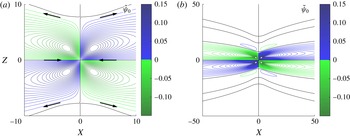
Figure 2 illustrates streamlines of the outer flow, and shows circulated fluid motion in each quadrant that is fastest close to the origin and directed in the same manner as near the cylinder in figure 1(b), but with no evidence of the flow reversal and a zero streamline at
 $r_{0}$
in this case. In effect, the cylindrical object in the outer region is represented by a point density disturbance at the origin. For the results shown here, the overall volume flux generated is
 $\max \{|\tilde{\unicode[STIX]{x1D713}}_{0}|\}\approx 0.1588$
, located near
 $(X,Z)=(\pm 2.36,\pm 2.12)$
, with maximum velocity components of
 $|\tilde{u} _{0}|\approx 0.1438$
and
 $|\tilde{w}_{0}|\approx 0.1469$
located nearby on the
 $X$
and
 $Z$
axes, respectively. One advantage of the integral form of the solutions (4.20) and (4.21) is that they can be evaluated accurately at individual points relatively easily, in contrast to a more typical approach of solving the governing equations (4.6) numerically. That said, to provide additional confidence that the analytical solutions presented here are correct, Alias (Reference Alias2015) also compared them with second-order finite-difference numerical solutions of (4.6) subject to (4.8b
) and with appropriate symmetry conditions on
 $X=0$
and
 $Z=0$
; those results confirmed all of the key features noted above, including the contour shapes as well as the size and locations of the extrema.
From figure 2(b) it is clear that the motion in the outer-flow region extends far from its forcing at the origin, especially in the
 $X$
direction. The far-field motion decays rapidly as
 $|Z|$
increases but relatively slowly in
 $X$
, although note the small recirculating regions near
 $Z=\pm 10$
. Indeed, the broad horizontal orientation of the streamlines in figure 2(b) is consistent with the stratification constraining vertical fluid motion (Tritton Reference Tritton1988, p. 197). Similar horizontal-oriented contours have also been observed in a similar contexts by Zagumennyi & Chashechkin (Reference Zagumennyi and Chashechkin2013c
) for an unsteady flow, as well as the so-called
 $R^{1/3}$
layers described by Page (Reference Page2011b
) for example, although in those cases the region is much thinner than the size of the object.
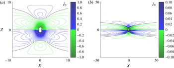
Contour plots of the leading-order density perturbation
 $\tilde{\unicode[STIX]{x1D70C}}_{0}$
from (4.21) in the outer region
 $(X,Z)$
over (a)
 $-10\leqslant \{X,Z\}\leqslant 10$
and (b) for
 $-50\leqslant \{X,Z\}\leqslant 50$
. The contour intervals are 0.01 and 0.0025, respectively (up to absolute values of one).

Figure 3 shows the density perturbation
 $\tilde{\unicode[STIX]{x1D70C}}_{0}$
, which is largest near the origin as a result of the inner matching condition (4.8b
). The perturbation density is consistent with bending of isopycnals that is evident near the cylinder for the inner solution
 $\unicode[STIX]{x1D70C}_{0}$
in figure 1(a), although recall the linear ‘background’ density profile is not part of
 $\tilde{\unicode[STIX]{x1D70C}}_{0}$
. For the results shown, the departure
 $|\tilde{\unicode[STIX]{x1D70C}}_{0}+Z/R^{2}|$
from the inner matching condition has a maximum of 0.2654 on the
 $Z$
axis near
 $(X,Z)=(0,\pm 3.24)$
, and a maximum
 $Z$
gradient of 0.1666 at the origin. As radius increases, the density perturbation
 $\tilde{\unicode[STIX]{x1D70C}}_{0}$
decreases in magnitude, again with relatively slow decay in the
 $X$
direction due to buoyancy forces that aim to restore the ‘deflected’ fluid to its neutral buoyant position.
The gradual spread in the
 $Z$
extent of
 $\tilde{\unicode[STIX]{x1D713}}_{0}$
in figure 2(b) and
 $\tilde{\unicode[STIX]{x1D70C}}_{0}$
in figure 3(b) as
 $X$
increases will be seen in § 4.3 to correspond to their far-field asymptotic behaviour, which can be represented in terms of the similarity variable
 $Z/X^{1/3}$
.
4.2 Asymptotic behaviour for
$R\ll 1$

To complete and verify the expected matching between the inner and outer regions, asymptotic solutions at small outer radius
 $R=\sqrt{X^{2}+Z^{2}}\ll 1$
will be derived, assuming here that
 $\unicode[STIX]{x1D6FC}>0$
for simplicity. This matching also determines some of the unidentified constants in the inner solutions described in § 3. Asymptotic solutions of streamfunction and density perturbation for
 $R\ll 1$
are derived by finding approximations of
 $S$
and
 $T$
for
 $\unicode[STIX]{x1D6FC}\gg 1$
from (4.13), from which expansions for
 $\unicode[STIX]{x1D6FD}_{n}$
follow from (4.12). For example, the asymptotic behaviour of
 $F_{n}(\unicode[STIX]{x1D6FC})$
from (4.19) can be expanded in inverse powers in a Laurent series
 $$\begin{eqnarray}\displaystyle & \displaystyle F_{1}=-\frac{\text{i}\unicode[STIX]{x03C0}\unicode[STIX]{x1D6FC}^{-1/3}}{3}\left(1+\frac{\unicode[STIX]{x1D6FC}^{-4/3}}{3}-\frac{5\unicode[STIX]{x1D6FC}^{-4}}{81}\right)+O(\unicode[STIX]{x1D6FC}^{-17/3}), & \displaystyle\end{eqnarray}$$
 $$\begin{eqnarray}\displaystyle & \displaystyle F_{2,3}=\frac{\text{i}\unicode[STIX]{x03C0}(1\pm \text{i}\sqrt{3})\unicode[STIX]{x1D6FC}^{-1/3}}{6}\left(1-\frac{(1\pm \text{i}\sqrt{3})\unicode[STIX]{x1D6FC}^{-4/3}}{6}-\frac{5\unicode[STIX]{x1D6FC}^{-4}}{81}\right)+O(\unicode[STIX]{x1D6FC}^{-17/3}), & \displaystyle\end{eqnarray}$$
with the equivalent for
 $G_{n}$
following from (4.15), and
 $$\begin{eqnarray}\unicode[STIX]{x1D706}_{1}=\unicode[STIX]{x1D6FC}-\unicode[STIX]{x1D6FC}^{-1/3}/2+\unicode[STIX]{x1D6FC}^{-5/3}/24+O(\unicode[STIX]{x1D6FC}^{-3})\end{eqnarray}$$
with
 $$\begin{eqnarray}\unicode[STIX]{x1D706}_{2,3}=\unicode[STIX]{x1D6FC}+(1\pm \text{i}\sqrt{3})\unicode[STIX]{x1D6FC}^{-1/3}/4-(1\mp \text{i}\sqrt{3})\unicode[STIX]{x1D6FC}^{-5/3}/48+O(\unicode[STIX]{x1D6FC}^{-3}).\end{eqnarray}$$
It is anticipated that these expressions converge for real values of
 $\unicode[STIX]{x1D6FC}$
larger than
 $(4/27)^{1/4}$
, based on the location in the complex plane of zeroes of the denominator of all
 $F_{n}(\unicode[STIX]{x1D6FC})$
, taking into account branch points of
 $\unicode[STIX]{x1D706}_{n}(\unicode[STIX]{x1D6FC})$
within that radius.
Using the above, series expansions of
 $A_{0}$
and
 $B_{0}$
valid for
 $\unicode[STIX]{x1D6FC}\gg 1$
and
 $0<X\ll 1$
are
 $$\begin{eqnarray}\displaystyle & \displaystyle A_{0}(X,\unicode[STIX]{x1D6FC})\sim -\text{i}\unicode[STIX]{x03C0}\bigg(\frac{X}{8\unicode[STIX]{x1D6FC}^{2}}-\frac{3X}{256\unicode[STIX]{x1D6FC}^{6}}+\frac{X^{2}}{8\unicode[STIX]{x1D6FC}}-\frac{3X^{2}}{256\unicode[STIX]{x1D6FC}^{5}}-\frac{X^{3}}{256\unicode[STIX]{x1D6FC}^{4}}+\frac{X^{5}}{3840\unicode[STIX]{x1D6FC}^{2}}\bigg)\text{e}^{-\unicode[STIX]{x1D6FC}X}, & \displaystyle\end{eqnarray}$$
 $$\begin{eqnarray}\displaystyle & \displaystyle B_{0}(X,\unicode[STIX]{x1D6FC})\sim \text{i}\unicode[STIX]{x03C0}\bigg(1-\frac{1}{16\unicode[STIX]{x1D6FC}^{4}}-\frac{X}{16\unicode[STIX]{x1D6FC}^{3}}+\frac{X^{3}}{48\unicode[STIX]{x1D6FC}}\bigg)\text{e}^{-\unicode[STIX]{x1D6FC}X}, & \displaystyle\end{eqnarray}$$
where
 $\text{e}^{-\unicode[STIX]{x1D6FC}X}$
(which arises from
 $\text{e}^{-\unicode[STIX]{x1D706}X}$
since
 $\unicode[STIX]{x1D706}\sim \unicode[STIX]{x1D6FC}$
) is retained in these expansions to ensure uniformity and so that they match (4.17a,b
). Sufficient terms are included above to ensure accurate inversion up to
 $O(R^{6})$
when
 $R$
is small. Note that all expressions above assume
 $\unicode[STIX]{x1D6FC}>0$
and
 $X>0$
but can be extended to other values by inclusion of relevant factors of
 $\text{sgn}(\unicode[STIX]{x1D6FC})$
and/or
 $\text{sgn}(X)$
, noting that
 $A_{0}$
is odd in both variables while
 $B_{0}$
is odd in
 $\unicode[STIX]{x1D6FC}$
and even in
 $X$
.
To facilitate the exact inversion of these approximations for
 $A_{0}$
and
 $B_{0}$
, using (4.20) and (4.21), the improper integral
 $$\begin{eqnarray}I_{k}(X,Z)=\int _{0}^{\infty }\unicode[STIX]{x1D6FC}^{-k}\text{e}^{-\unicode[STIX]{x1D6FC}|X|}\sin (\unicode[STIX]{x1D6FC}Z)\,\text{d}\unicode[STIX]{x1D6FC}\quad \text{for }k\geqslant 0\end{eqnarray}$$
is introduced here for any
 $(X,Z)$
and integer values of
 $k$
. Although these integrals do not exist in the usual sense for
 $k\geqslant 2$
, and arguably the inverse transforms should also include contributions from
 $A_{0}$
and
 $B_{0}$
at smaller values of
 $\unicode[STIX]{x1D6FC}$
than where (4.26) and (4.27) apply, they can be interpreted and evaluated in the ‘generalised function’ sense of Lighthill (Reference Lighthill1958), for example. Further explanation of this approach, including an outline of how to derive expressions for (4.28) up to
 $k=4$
, is provided in the appendix. Values of
 $I_{k}(X,Z)$
for larger
 $k$
are listed in Alias (Reference Alias2015).
A series expansion for
 $\tilde{\unicode[STIX]{x1D713}}_{0}(X,Z)$
for
 $R\ll 1$
can then be obtained as
 $$\begin{eqnarray}\displaystyle \tilde{\unicode[STIX]{x1D713}}_{0}(X,Z) & = & \displaystyle \frac{X}{8}I_{2}-\frac{3X}{256}I_{6}+\frac{X^{2}}{8}I_{1}-\frac{3X^{2}}{256}I_{5}-\frac{X^{3}}{256}I_{4}+\frac{X^{5}}{3840}I_{2}+\cdots \nonumber\\ \displaystyle & = & \displaystyle -\frac{XZ}{8}\ln R-\frac{C_{1}XZ}{8}+\frac{(3XZ^{5}+10X^{3}Z^{3}+7X^{5}Z)\ln R}{30~720}\nonumber\\ \displaystyle & & \displaystyle +\,\frac{(28C_{1}-17)X^{5}Z}{122~880}+\frac{(20C_{2}-3)X^{3}Z^{3}}{61~440}+\frac{C_{3}XZ^{5}}{10~240}+O(R^{10}).\end{eqnarray}$$
The first term in this matches with (4.8a
), even though that matching condition was not used directly in its determination. All of the
 $\arctan (Z/X)$
terms arising in the
 $I_{k}(X,Z)$
cancel here, so
 $\tilde{\unicode[STIX]{x1D713}}_{0}(X,Z)$
has no corresponding discontinuities in the
 $(X,Z)$
plane.
Similarly,
 $\tilde{\unicode[STIX]{x1D70C}}_{0}(X,Z)$
for
 $R\ll 1$
is given by
 $$\begin{eqnarray}\displaystyle \tilde{\unicode[STIX]{x1D70C}}_{0}(X,Z) & = & \displaystyle -I_{0}+\frac{1}{16}I_{4}+\frac{X}{16}I_{3}-\frac{X^{3}}{48}I_{1}+\cdots \nonumber\\ \displaystyle & = & \displaystyle -\frac{Z}{R^{2}}+\frac{C_{2}Z^{3}}{96}+\frac{(6C_{1}-1)X^{2}Z}{192}+\frac{(Z^{3}+3X^{2}Z)\ln R}{96}+O(R^{7}),\end{eqnarray}$$
which matches with (4.8b
) as expected, again without any
 $\arctan (Z/X)$
terms present.
Here
 $C_{1}$
,
 $C_{2}$
and
 $C_{3}$
are constants that in principle are determined by the full exact expressions for
 $A_{0}$
and
 $B_{0}$
when (4.20) and (4.21) are evaluated over all
 $\unicode[STIX]{x1D6FC}$
, rather than based on (4.26) and (4.27) for
 $\unicode[STIX]{x1D6FC}>(4/27)^{1/4}$
. Indeed, one interpretation is that they arise from contributions to the Fourier inversion integral over
 $0<\unicode[STIX]{x1D6FC}<(4/27)^{1/4}$
that are not taken into account in individual terms of (4.26) and (4.27).
That said, the two constants
 $C_{2}$
and
 $C_{3}$
here can be identified by ensuring consistency between the asymptotic solutions, as for example substituting (4.29) and (4.30) into (4.6) requires that
 $C_{2}=C_{1}-5/6$
and
 $C_{3}=C_{1}-77/60$
. The value of
 $C_{1}$
cannot be identified in this manner although from (4.29) it clearly relates to
 $\unicode[STIX]{x2202}^{2}\tilde{\unicode[STIX]{x1D713}}_{0}/\unicode[STIX]{x2202}X\unicode[STIX]{x2202}Z$
when
 $R\ll 1$
. Differentiating (4.20) and (4.29) with respect to
 $X$
and
 $Z$
, and evaluating at
 $Z=0$
, gives
 $$\begin{eqnarray}\frac{\unicode[STIX]{x2202}^{2}\tilde{\unicode[STIX]{x1D713}}_{0}}{\unicode[STIX]{x2202}X\unicode[STIX]{x2202}Z}(X,0)=-\frac{\text{i}}{\unicode[STIX]{x03C0}}\int _{0}^{\infty }\mathop{\sum }_{n=1}^{3}\unicode[STIX]{x1D6FC}\unicode[STIX]{x1D706}_{n}F_{n}\text{e}^{-\unicode[STIX]{x1D706}_{n}X}\text{d}\unicode[STIX]{x1D6FC}=-\frac{1}{8}\ln X-\frac{C_{1}}{8}-\frac{1}{8}+O(X^{4})\end{eqnarray}$$
for
 $0<X\ll 1$
, which implies that
 $$\begin{eqnarray}C_{1}=\lim _{X\rightarrow 0+}\bigg(\frac{8\text{i}}{\unicode[STIX]{x03C0}}\int _{0}^{\infty }\mathop{\sum }_{n=1}^{3}\unicode[STIX]{x1D6FC}\unicode[STIX]{x1D706}_{n}F_{n}\text{e}^{-\unicode[STIX]{x1D706}_{n}X}\,\text{d}\unicode[STIX]{x1D6FC}-1-\ln X\bigg)\approx -1.087505.\end{eqnarray}$$
The estimated value of
 $C_{1}$
in (4.32) was found numerically using the full expressions for
 $\unicode[STIX]{x1D706}_{n}$
as a functions of
 $\unicode[STIX]{x1D6FC}$
as well as
 $F_{n}(\unicode[STIX]{x1D6FC})$
from (4.19), using a similar method to that described in § 4.1. This integral (4.31) converges slowly for large values of
 $\unicode[STIX]{x1D6FC}$
, arising from the
 $O(1/\unicode[STIX]{x1D6FC})$
behaviour of
 $\unicode[STIX]{x1D6FC}$
times the first term in (4.26), but this can be ameliorated by subtracting a corresponding multiple of
 $H(\unicode[STIX]{x1D6FC}-1)\exp (-\unicode[STIX]{x1D6FC}X)/\unicode[STIX]{x1D6FC}$
from the integrand, where
 $H$
is the Heaviside step function. This subtracted contribution can be evaluated exactly in terms of the exponential integral
 $\text{Ei}(-X)$
, and both significantly improves the decay rate of the integrand to
 $O(1/\unicode[STIX]{x1D6FC}^{5})$
when
 $\unicode[STIX]{x1D6FC}$
is large and accurately offsets the
 $\ln X$
term in the limit.
4.2.1 Inner–outer matching
The asymptotic form (4.29) of the outer solution, expressed in polar coordinates
 $(R,\unicode[STIX]{x1D703})$
for
 $R\ll 1$
and using
 $C_{2}$
and
 $C_{3}$
as determined above, is
 $$\begin{eqnarray}\displaystyle \tilde{\unicode[STIX]{x1D713}}(R,\unicode[STIX]{x1D703}) & = & \displaystyle -\bigg(C_{1}+\ln R\bigg)\frac{R^{2}\sin 2\unicode[STIX]{x1D703}}{16}+\bigg(C_{1}-\frac{7}{8}+\ln R\bigg)\frac{R^{6}\sin 2\unicode[STIX]{x1D703}}{12~288}\nonumber\\ \displaystyle & & \displaystyle -\,\bigg(C_{1}-\frac{1}{10}+\ln R\bigg)\frac{R^{6}\sin 4\unicode[STIX]{x1D703}}{61~440}+\frac{13R^{6}\sin 6\unicode[STIX]{x1D703}}{7~372~800}+O(R^{10}),\end{eqnarray}$$
and (4.30) gives that
 $$\begin{eqnarray}\tilde{\unicode[STIX]{x1D70C}}(R,\unicode[STIX]{x1D703})=\frac{-\!\cos \unicode[STIX]{x1D703}}{R}+\bigg(C_{1}-\frac{1}{2}+\ln R\bigg)\frac{R^{3}\cos \unicode[STIX]{x1D703}}{64}-\bigg(C_{1}+\frac{1}{6}+\ln R\bigg)\frac{R^{3}\cos 3\unicode[STIX]{x1D703}}{192}+O(R^{7}).\end{eqnarray}$$
Noting that
 $\ln r=(\ln R-\ln \unicode[STIX]{x1D6FF})$
,
 $\unicode[STIX]{x1D713}(r,\unicode[STIX]{x1D703})=\tilde{\unicode[STIX]{x1D713}}(r\unicode[STIX]{x1D6FF},\unicode[STIX]{x1D703})/\unicode[STIX]{x1D6FF}^{2}$
and
 $\unicode[STIX]{x1D6FF}^{4}=\unicode[STIX]{x1D70E}\unicode[STIX]{x1D716}$
, each term in (4.33) can be matched with the large
 $r$
behaviour of (3.4) and (3.9), requiring that
 $$\begin{eqnarray}c_{0}+\ln \unicode[STIX]{x1D6FF}=-C_{1}\quad \text{with }-\!\left(\frac{d_{1}}{2}+\frac{c_{0}}{2}+\frac{23}{24}+\ln \unicode[STIX]{x1D6FF}\right)=C_{1}-\frac{7}{8}.\end{eqnarray}$$
This completes the determination of both unspecified constants in the leading-order inner streamfunction
 $\unicode[STIX]{x1D713}_{0}$
(3.4) and second-order inner density perturbation
 $\unicode[STIX]{x1D70C}_{1}$
(3.7), with
 $$\begin{eqnarray}c_{0}=-C_{1}-\ln \unicode[STIX]{x1D6FF}\quad \text{and}\quad d_{1}=c_{0}-{\textstyle \frac{1}{6}},\end{eqnarray}$$
both given in terms of
 $C_{1}$
at (4.32). It also confirms the presence of
 $\ln \unicode[STIX]{x1D6FF}$
terms in both
 $\unicode[STIX]{x1D713}_{0}$
and
 $\unicode[STIX]{x1D70C}_{1}$
, and hence more generally in the inner expansions (3.1). A similar matching process yields that
 ${\hat{c}}_{14}=c_{0}+9/10$
and
 $c_{16}=13/7\,372\,800$
for the largest terms in (3.9).
Any remaining undetermined constants (such as
 $c_{12}$
,
 ${\hat{c}}_{12}$
and
 $c_{14}$
in
 $\unicode[STIX]{x1D713}_{1}$
) will require that higher-order
 $O(\unicode[STIX]{x1D6FF}^{2})$
solutions be found in the outer region, but the lack of closed-form solutions for
 $\tilde{\unicode[STIX]{x1D70C}}_{0}$
and
 $\tilde{\unicode[STIX]{x1D713}}_{0}$
, and the nonlinearity of (4.4) and (4.5), make that problem unlikely to be tractable using the same approach as in this paper. An asymptotic matching approach, perhaps linked with numerical solutions, may yield some success but that possibility has not been pursued here as the main intent of this study has been to demonstrate the leading-order matching.
Since
 $c_{0}$
is positive, and the value of
 $r_{0}\approx \exp (c_{0})$
is
 $O(1/\unicode[STIX]{x1D6FF})$
, it follows that reversing of the inner-layer flow as indicated in figure 1(b) will not occur when
 $\unicode[STIX]{x1D6FF}\ll 1$
. Also, the leading-order inner solution
 $\unicode[STIX]{x1D713}_{0}$
comprises two parts, one involving constants only and the other proportional to
 $\ln \unicode[STIX]{x1D6FF}$
; through the nonlinear terms on the right-hand sides of (3.5) and (3.6), these both force terms proportional to
 $\ln \unicode[STIX]{x1D6FF}$
in
 $\unicode[STIX]{x1D70C}_{1}$
and up to quadratic powers of
 $\ln \unicode[STIX]{x1D6FF}$
in
 $\unicode[STIX]{x1D713}_{1}$
. That the value of
 $c_{16}$
above, for example, involves no
 $\ln \unicode[STIX]{x1D6FF}$
component relates to the absence of any
 $r^{6}\ln r$
terms being forced in
 $\unicode[STIX]{x1D713}_{1}$
through the right-hand side of (3.5).
The largest terms in the outer and inner solutions for the density perturbation (4.34) and (3.7), with
 $\bar{\unicode[STIX]{x1D70C}}=\unicode[STIX]{x1D6FF}\tilde{\unicode[STIX]{x1D70C}}$
, also match using the values of
 $c_{0}$
and
 $d_{1}$
determined above. That this matching is able to be performed up to second order for both variables in the inner region, even though the outer solution is forced by the single matching condition (4.8b
), gives confidence that the asymptotic structure and analysis are correct. It is pertinent that Candelier et al. (Reference Candelier, Mehaddi and Vauquelin2014) undertook a similar two-region matching for unsteady motion due to a descending sphere, although in terms of a multiply Fourier transformed solution.
4.3 Asymptotic behaviour for
$R\gg 1$

Using the same process as in § 4.2 but for
 $0<\unicode[STIX]{x1D6FC}\ll 1$
, the corresponding approximate forms for
 $\unicode[STIX]{x1D706}_{n}$
and
 $F_{n}$
when
 $X>0$
can be obtained as
 $$\begin{eqnarray}\unicode[STIX]{x1D706}_{1}=\unicode[STIX]{x1D6FC}^{3}-\frac{3\unicode[STIX]{x1D6FC}^{7}}{2}+O(\unicode[STIX]{x1D6FC}^{11})\quad \text{with }\unicode[STIX]{x1D706}_{2,3}=\frac{1\pm \text{i}}{\sqrt{2}}\bigg(1\mp \frac{3\text{i}\unicode[STIX]{x1D6FC}^{2}}{4}+\frac{15\unicode[STIX]{x1D6FC}^{4}}{32}\bigg)+O(\unicode[STIX]{x1D6FC}^{6})\end{eqnarray}$$
and after simplification that
 $$\begin{eqnarray}F_{1}=\text{i}\unicode[STIX]{x03C0}(-\unicode[STIX]{x1D6FC}+3\unicode[STIX]{x1D6FC}^{5}-15\unicode[STIX]{x1D6FC}^{9})+O(\unicode[STIX]{x1D6FC}^{13}),\quad F_{2,3}=\text{i}\unicode[STIX]{x03C0}\bigg(\frac{\unicode[STIX]{x1D6FC}}{2}\pm \frac{3\text{i}\unicode[STIX]{x1D6FC}^{3}}{4}-\frac{3\unicode[STIX]{x1D6FC}^{5}}{2}\bigg)+O(\unicode[STIX]{x1D6FC}^{7}).\quad\end{eqnarray}$$
Based on these, the leading terms in
 $A_{0}$
and
 $B_{0}$
for small
 $\unicode[STIX]{x1D6FC}$
can be determined as
 $$\begin{eqnarray}A_{0}(X,\unicode[STIX]{x1D6FC})=-\text{i}\unicode[STIX]{x03C0}\unicode[STIX]{x1D6FC}\text{e}^{-\unicode[STIX]{x1D6FC}^{3}X}+O(\unicode[STIX]{x1D6FC}^{4})\quad \text{and}\quad B_{0}(X,\unicode[STIX]{x1D6FC})=\text{i}\unicode[STIX]{x03C0}\unicode[STIX]{x1D6FC}^{2}\text{e}^{-\unicode[STIX]{x1D6FC}^{3}X}+O(\unicode[STIX]{x1D6FC}^{5}),\end{eqnarray}$$
where terms involving
 $\exp (-\unicode[STIX]{x1D706}_{2}X)$
and
 $\exp (-\unicode[STIX]{x1D706}_{3}X)$
are neglected as they approach zero more rapidly when
 $X$
is large. Asymptotic approximations for the streamfunction (4.20) and density perturbation (4.21) at large values of
 $(X,Z)$
are therefore given by
 $$\begin{eqnarray}\tilde{\unicode[STIX]{x1D713}}_{0}(X,Z)\sim \int _{0}^{\infty }\unicode[STIX]{x1D6FC}\text{e}^{-\unicode[STIX]{x1D6FC}^{3}X}\sin (\unicode[STIX]{x1D6FC}Z)\,\text{d}\unicode[STIX]{x1D6FC}\end{eqnarray}$$
and
 $$\begin{eqnarray}\tilde{\unicode[STIX]{x1D70C}}_{0}(X,Z)\sim -\int _{0}^{\infty }\unicode[STIX]{x1D6FC}^{2}\text{e}^{-\unicode[STIX]{x1D6FC}^{3}X}\sin (\unicode[STIX]{x1D6FC}Z)\,\text{d}\unicode[STIX]{x1D6FC}.\end{eqnarray}$$
Exact expressions for these integrals are not available, but they can be approximated numerically using the same approach as described in § 4.1. Plots of those show very similar features to figures 2(b) and 3(b), especially for
 $R\gg 1$
where they should correspond. This includes the narrow regions where
 $\tilde{\unicode[STIX]{x1D713}}_{0}$
and
 $\tilde{\unicode[STIX]{x1D70C}}_{0}$
change signs as
 $Z$
increases at fixed
 $X$
, indicating relatively minor reversals in the direction of the flow at the outer edge of the region along as well as small secondary peaks in the density perturbation.
Although the integrals (4.40) and (4.41) cannot be evaluated analytically, further information on their asymptotic properties can be identified based on Moore & Saffman (Reference Moore and Saffman1969). In the context of a related problem in rotating-fluid flow, they determined the asymptotic behaviour of a class of complex-valued integrals of the form
 $$\begin{eqnarray}H_{M}(\unicode[STIX]{x1D70F})=\int _{0}^{\infty }p^{-3M-1}\text{e}^{-p^{3}}\text{e}^{-\text{i}p\unicode[STIX]{x1D70F}}\,\text{d}p\sim (\pm \unicode[STIX]{x1D70F})^{3M}\text{exp}\left(\pm \frac{\text{i}3M\unicode[STIX]{x03C0}}{2}\right)(-3M-1)!\end{eqnarray}$$
as
 $\unicode[STIX]{x1D70F}\rightarrow \pm \infty$
where
 $M<0$
relates to the power of
 $X$
that appears in the assumed similarity solutions. Substituting
 $\unicode[STIX]{x1D6FC}=pX^{-1/3}$
and
 $Z=\unicode[STIX]{x1D70F}X^{1/3}$
, (4.40) becomes
 $$\begin{eqnarray}\tilde{\unicode[STIX]{x1D713}}_{0}(X,Z)\sim \frac{1}{X^{2/3}}\int _{0}^{\infty }p\text{e}^{-p^{3}}\sin (p\unicode[STIX]{x1D70F})\,\text{d}p=-\frac{1}{X^{2/3}}\text{Im}\{H_{-2/3}(\unicode[STIX]{x1D70F})\},\end{eqnarray}$$
where
 $\text{Im}\{H_{-2/3}(\unicode[STIX]{x1D70F})\}$
is the imaginary part of (4.42) with
 $M=-2/3$
. Correspondingly,
 $$\begin{eqnarray}\tilde{\unicode[STIX]{x1D70C}}_{0}(X,Z)\sim -\frac{1}{X}\int _{0}^{\infty }p^{2}\text{e}^{-p^{3}}\sin (p\unicode[STIX]{x1D70F})\,\text{d}p=\frac{1}{X}\text{Im}\{H_{-1}(\unicode[STIX]{x1D70F})\}\end{eqnarray}$$
for
 $M=-1$
, and the velocity component
 $\tilde{u} _{0}$
has the same form but involves
 $\cos$
rather than
 $\sin$
. Using (4.42), at the outer
 $Z$
extent of this region it can be shown that
 $$\begin{eqnarray}\tilde{\unicode[STIX]{x1D713}}_{0}(X,Z)\sim -\frac{24X}{Z^{5}}\quad \text{and}\quad \tilde{\unicode[STIX]{x1D70C}}_{0}(X,Z)\sim \frac{2}{Z^{3}}\end{eqnarray}$$
for large
 $\unicode[STIX]{x1D70F}$
, where the higher-order expression for
 $\unicode[STIX]{x1D713}_{0}$
can be obtained by comparing the
 $X$
derivative of (4.40) with the second
 $Z$
derivative of (4.41). The expressions (4.45) clearly indicate that the far-field solutions decay algebraically for
 $Z\gg X^{1/3}$
, rather than exponentially.
More generally, the form of (4.43) and (4.44) verifies that all dependent variables in the far field, at large
 $(X,Z)$
, can be written as similarity solutions to leading order, in terms of
 $\unicode[STIX]{x1D70F}=Z/X^{1/3}$
. This behaviour is consistent with the gradual spreading apparent in figures 2(b) and 3(b). The form of
 $\unicode[STIX]{x1D70F}$
also accords with the large-
 $X$
case of (4.7) in which
 $\tilde{\unicode[STIX]{x1D6FB}}^{6}$
is replaced by
 $\unicode[STIX]{x2202}^{6}/\unicode[STIX]{x2202}Z^{6}$
. Further, as the asymptotic forms of
 $\tilde{\unicode[STIX]{x1D713}}_{0}$
and
 $\tilde{\unicode[STIX]{x1D70C}}_{0}$
are derived here from the exact solution in the outer region, both the correct values of
 $M$
and the relevant multiples of
 $H_{M}(\unicode[STIX]{x1D70F})$
can be identified unambiguously.
Related similarity solutions in
 $\unicode[STIX]{x1D70F}$
were described by Koh (Reference Koh1966) for a point source in a viscous stratified fluid, corresponding to
 $M=-1/3$
for both the horizontal velocity and density, and in that case there was a small region of reversed flow direction at the outer edge of the layer, as also observed above. The same solution was used to describe the so-called ‘
 $R^{1/3}$
layers’ in diffusion-driven motion for contained flows at high Rayleigh numbers (Page & Johnson Reference Page and Johnson2008, Reference Page and Johnson2009), for which
 $\unicode[STIX]{x1D6FF}={\mathcal{R}}^{1/2}$
. The
 $M=-2/3$
case arose in Page (Reference Page2011b
) when describing high-order effects that occur for ‘corner-induced flows’, and more recently has been shown to be relevant to external corners in a similar context. This latter type of flow also accords with the large
 $X$
case of the two-dimensional ‘momentum jet’ considered by List (Reference List1971), for which the axisymmetric equivalent was described further by Ardekani & Stocker (Reference Ardekani and Stocker2010) and referred to as a ‘Stratlet’. Finally, Alias (Reference Alias2015) shows that far-field horizontal velocity and density perturbations due to the slow vertical motion of a cylinder can be represented using
 $M=-4/3$
in (4.42).
5 Remarks
The small-Reynolds-number
 $\unicode[STIX]{x1D716}\ll 1$
external flow considered here is novel in comparison with previous studies of diffusion-driven flows, which concentrate on the high-Rayleigh-number case where the effect is driven by a thin boundary layer of thickness of
 $O({\mathcal{R}}^{1/2})$
and in particular contained flows. Streamfunction and density fields were determined analytically using a two-region approach: the inner region describes the obstacle-scale effects, and solutions are found to not satisfy the far-field conditions, while the outer region is of relative size
 $O(1/\unicode[STIX]{x1D6FF})$
, where
 $\unicode[STIX]{x1D6FF}=(\unicode[STIX]{x1D70E}\unicode[STIX]{x1D716})^{1/4}\ll 1$
. This structure is analogous to the typical approach for low-Reynolds-number homogeneous flows, but here the size of the outer region is determined through a dynamical balance between viscous and buoyancy terms. In dimensional terms this outer region has size
 $(\unicode[STIX]{x1D705}^{\ast }\unicode[STIX]{x1D708}^{\ast }/N^{\ast 2})^{1/4}$
, equivalent to that noted by Ardekani & Stocker (Reference Ardekani and Stocker2010) for example in a slightly different context. The leading-order solutions in these two regions were determined analytically here, and then successfully matched together (enabling all of the unspecified constants to be determined). This provides some confidence in the appropriateness of the two-region structure. Asymptotic expressions for the exact outer solution were determined directly, and one further advantage of the exact solutions for (4.20) and (4.21) in the outer flow is that their point-wise values can be evaluated with relatively little effort.
The circular cylindrical body examined here allows exact analytical expressions to be obtained for the streamfunction and density fields in the outer-flow region, but the main features of that motion will be similar for more complicated bodies in the same parameter regime. This is due to the leading-order outer flow in § 4 being principally driven by the
 $O(1/R)$
perturbation in the density near
 $R=0$
, which is the most slowly decaying term at the outer edge of the inner region. It is postulated here that a similar term would be expected to be present in the far-field density expansion for almost any two-dimensional closed object in the
 $(x,z)$
plane with generators along the
 $y$
axis. In that case the leading-order outer flow is effectively independent of most of the finer-detailed features of the inner solution.
The asymptotic structure used here can also be applied to the corresponding flow with spherical symmetry when
 $\unicode[STIX]{x1D716}\ll 1$
. Similar exact solutions in the outer region are not currently available in that case (Alias Reference Alias2015), but numerical solutions of the outer-region equations can be used with some confidence. The details are different but inner
 $R=O(1)$
and outer
 $R=O(1/\unicode[STIX]{x1D6FF})$
regions can be formulated similarly, with leading-order outer-flow velocities of
 $O(1/\unicode[STIX]{x1D6FF})$
driven by an
 $O(1/R^{2})$
density perturbation when the spherical radius
 $R$
is small. Candelier et al. (Reference Candelier, Mehaddi and Vauquelin2014) consider an unsteady problem in that context, but using quadruple Fourier transforms.
A further extension of the analysis here might consider in more detail the large
 $\unicode[STIX]{x1D70E}$
case, rather than assuming throughout that
 $\unicode[STIX]{x1D70E}=O(1)$
with respect to
 $\unicode[STIX]{x1D716}\ll 1$
. For example,
 $\unicode[STIX]{x1D70E}=O(\unicode[STIX]{x1D716}^{-1/2})$
is arguably more appropriate for salt-stratified water, for which
 $\unicode[STIX]{x1D70E}=10^{3}$
and
 $\unicode[STIX]{x1D716}=10^{-6}$
(see below). However, since all terms in
 $\unicode[STIX]{x1D713}_{1}$
that are multiplied by
 $\unicode[STIX]{x1D70E}$
are retained in the leading-order matching performed in § 4.2.1, it is expected that the principal results here remain valid for large
 $\unicode[STIX]{x1D70E}$
. Indeed, albeit in a slightly different context, Page (Reference Page2011a
) concluded that the analysis of diffusion-driven flows for large
 $\unicode[STIX]{x1D70E}$
is similar to when
 $\unicode[STIX]{x1D70E}$
is an order-one quantity, and perhaps simpler because some of the nonlinear terms are relatively small in that limit.
When
 $\unicode[STIX]{x1D716}\ll 1$
, and hence
 $\unicode[STIX]{x1D6FF}\ll 1$
also, the nonlinear terms in both the inner and outer regions are relatively small, of
 $O(\unicode[STIX]{x1D6FF}^{4})$
and
 $O(\unicode[STIX]{x1D6FF}^{2})$
respectively. Separate finite-difference numerical solutions of the nonlinear outer-flow equations (4.4) and (4.5) up to
 $\unicode[STIX]{x1D6FF}=1$
, obtained using a similar method to that mentioned in § 4.1 for the
 $\unicode[STIX]{x1D6FF}\ll 1$
case, indicate that the main qualitative features of the nonlinear outer flow are captured by the leading-order solution of the linear problem when
 $\unicode[STIX]{x1D6FF}=0$
. The leading-order flow in the outer region, driven here by an isolated point singularity, can therefore be extended to that due to a collection of numerous point disturbances using linear superposition when
 $\unicode[STIX]{x1D6FF}\ll 1$
, with some confidence that it should be representative for larger values of
 $\unicode[STIX]{x1D6FF}$
as well. Also, while a single symmetric object should remain stationary, Allshouse et al. (Reference Allshouse, Barad and Peacock2010) observe that multiple particles can be expected to induce relative motion. The effect of say
 $10^{6}$
isolated particles within a region of radius
 $O(1/\unicode[STIX]{x1D6FF})$
would magnify that considerably.
The implications on the motion of clouds of small objects in an ocean, for example ‘hair-like’ strands or even so-called ‘marine snow’, can be estimated by calculating the scale speed of the induced motion for typical parameter values. For a relative density gradient
 $\unicode[STIX]{x1D70C}_{0}^{\prime \ast }/\unicode[STIX]{x1D70C}_{00}^{\ast }$
in the ocean of say
 $10^{-3}$
m
 $^{-1}$
, and
 $\unicode[STIX]{x1D708}^{\ast }=10^{-6}$
m
 $^{2}$
s
 $^{-1}$
for water in SI units, the Reynolds number (2.2) is at most
 $\unicode[STIX]{x1D716}=10^{-6}$
for so-called microparticles of size up to
 $a^{\ast }=100~\unicode[STIX]{x03BC}\text{m}$
(Ardekani & Stocker Reference Ardekani and Stocker2010). This decreases in proportion to
 ${a^{\ast }}^{4}$
for smaller objects, so clearly the small-Reynolds-number assumption is appropriate in these circumstances. For either temperature-stratified (
 $\unicode[STIX]{x1D70E}=10$
) or salt-stratified (
 $\unicode[STIX]{x1D70E}=10^{3}$
) water, the outer region is significantly larger than the particles by a factor of
 $O(1/\unicode[STIX]{x1D6FF})$
, or say 10 at least. Based on the scaling at (4.1), the maximum dimensional velocities in the outer region are of order
 $(\unicode[STIX]{x1D708}^{\ast }\unicode[STIX]{x1D716}/\unicode[STIX]{x1D6FF}a^{\ast })$
, which is about
 $10^{-7}$
m s
 $^{-1}$
or a distance of
 $a^{\ast }$
every fifteen minutes. The outer flow in §4 extends horizontally over a broad region of at least
 $10/\unicode[STIX]{x1D6FF}$
, or
 $100a^{\ast }$
, so this induced motion could be further magnified locally by superposition. That said, in a paper on swimming microorganisms, Wagner et al. (Reference Wagner, Young and Lauga2014) note that relevant local density gradients in the ocean may be larger than those used above and hence
 $\unicode[STIX]{x1D716}$
is up to 200 times larger and
 $1/\unicode[STIX]{x1D6FF}$
smaller. In such situations diffusion-driven flow may not ever be a principal driver of relative particle motion in a cloud of microparticles, but arguably it might not be negligible in a sheltered environment.
Acknowledgements
The authors are grateful to a referee for their very helpful comments, including identifying some typographical and calculation errors in the first draft of this paper.
Appendix A
The process used in § 4.2 to evaluate the integrals
 $$\begin{eqnarray}I_{k}(X,Z)=\int _{0}^{\infty }\unicode[STIX]{x1D6FC}^{-k}\exp (-\unicode[STIX]{x1D6FC}X)\sin (\unicode[STIX]{x1D6FC}Z)\,\text{d}\unicode[STIX]{x1D6FC}\quad \text{for }k\geqslant 0\end{eqnarray}$$
at (4.28) when
 $X\geqslant 0$
and
 $R=\sqrt{X^{2}+Z^{2}}\ll 1$
is described here in more detail. For
 $k=0$
and
 $k=1$
, the improper integral exists in the normal sense and has values
 $$\begin{eqnarray}I_{0}(X,Z)=\frac{Z}{X^{2}+Z^{2}}\quad \text{and}\quad I_{1}(X,Z)=\arctan \bigg(\frac{Z}{X}\bigg),\end{eqnarray}$$
where
 $I_{1}$
follows from integrating
 $I_{0}$
with respect to
 $X$
using that
 $$\begin{eqnarray}\frac{\unicode[STIX]{x2202}}{\unicode[STIX]{x2202}X}I_{k}(X,Z)=-I_{k-1}(X,Z)\quad \text{for }k\geqslant 1.\end{eqnarray}$$
For
 $k\geqslant 2$
, however, the integral
 $I_{k}(X,Z)$
does not exist in the normal sense of an improper integral due to the behaviour of the integrand near
 $\unicode[STIX]{x1D6FC}=0$
. However, such integrals can be evaluated based on a ‘generalised function’ interpretation of the integrand, see Chap. 4 of Lighthill (Reference Lighthill1958) or Chap. 9 of Jones (Reference Jones1966). Lighthill (p. 37) also notes that this approach relates to the ‘Cauchy principal value’ of such integrals.
Before proceeding, (A 1) at
 $X=0$
can be expressed equivalently over all real
 $\unicode[STIX]{x1D6FC}$
as
 $$\begin{eqnarray}I_{k}(0,Z)=\frac{\text{i}}{2}\left\{\begin{array}{@{}ll@{}}\displaystyle \int _{-\infty }^{\infty }\unicode[STIX]{x1D6FC}^{-k}\exp (-\text{i}\unicode[STIX]{x1D6FC}Z)\,\text{d}\unicode[STIX]{x1D6FC} & \text{for }k=\text{odd integer},\\ \displaystyle \int _{-\infty }^{\infty }\unicode[STIX]{x1D6FC}^{-k}\text{sgn}(\unicode[STIX]{x1D6FC})\exp (-\text{i}\unicode[STIX]{x1D6FC}Z)\,\text{d}\unicode[STIX]{x1D6FC} & \text{for }k=\text{even integer}.\end{array}\right.\end{eqnarray}$$
Using Lighthill’s Table 1 (p. 43) of Fourier transforms of the corresponding generalised functions, these integrals can be evaluated as
 $$\begin{eqnarray}I_{k}(0,Z)=\frac{(-\text{i})^{k-1}}{2(k-1)!}\left\{\begin{array}{@{}ll@{}}\unicode[STIX]{x03C0}Z^{k-1}\text{sgn}(Z) & \text{for }k=\text{odd integer},\\ -2\text{i}Z^{k-1}(\ln |Z|+C_{k/2}) & \text{for }k=\text{even integer},\end{array}\right.\end{eqnarray}$$
where
 $C_{k/2}$
is an undetermined constant (with a different value at each even integer
 $k$
). As noted by Lighthill (p. 39), in essence these constants arise due to the presence of unknown multiples of the Dirac delta function or its derivative in the inverse transform. In the context of terms in an expansion of some function
 $F(\unicode[STIX]{x1D6FC})$
for large
 $\unicode[STIX]{x1D6FC}$
, another possible interpretation is that these constants arise from properties of that function that are not able to be determined from individual terms in that expansion, for example integrals of
 $F(\unicode[STIX]{x1D6FC})$
over
 $O(1)$
values of
 $\unicode[STIX]{x1D6FC}$
.
When
 $k=2,3,4$
, for example, the values of (A 1) at
 $X=0$
are
 $$\begin{eqnarray}I_{2}(0,Z)=-Z(\ln |Z|+C_{1}),\quad I_{3}(0,Z)=\frac{-\unicode[STIX]{x03C0}Z^{2}}{4}\text{sgn}(Z),\quad I_{4}(0,Z)=\frac{Z^{3}}{6}(\ln |Z|+C_{2}),\end{eqnarray}$$
where
 $C_{1}$
and
 $C_{2}$
are arbitrary constants. For
 $X\geqslant 0$
, the recurrence (A 3) gives that
 $$\begin{eqnarray}I_{2}(X,Z)=-X\arctan \left(\frac{Z}{X}\right)-\frac{Z}{2}\ln (X^{2}+Z^{2})-C_{1}Z,\end{eqnarray}$$
where the last term is obtained from the
 $X=0$
result above, and likewise
 $$\begin{eqnarray}\displaystyle I_{3}(X,Z) & = & \displaystyle \frac{X^{2}-Z^{2}}{2}\arctan \left(\frac{Z}{X}\right)+\frac{XZ}{2}\ln (X^{2}+Z^{2})+\left(C_{1}-\frac{1}{2}\right)XZ,\end{eqnarray}$$
 $$\begin{eqnarray}\displaystyle I_{4}(X,Z) & = & \displaystyle \frac{X(3Z^{2}-X^{2})}{6}\arctan \left(\frac{Z}{X}\right)+\frac{Z(Z^{2}-3X^{2})}{12}\ln (X^{2}+Z^{2})\nonumber\\ \displaystyle & & \displaystyle +\,\left(\frac{5}{12}-\frac{C_{1}}{2}\right)X^{2}Z+\frac{C_{2}}{6}Z^{3}.\end{eqnarray}$$
Expressions for
 $I_{5}(X,Z)$
and
 $I_{6}(X,Z)$
used in § 4.2 can be found similarly (Alias Reference Alias2015).