1. Introduction
It is a great pleasure and privilege to be invited to contribute to this volume in honour of the centenary of the birth of Professor Ya. B. Zel’dovich. Zel’dovich’s research interests were so wide ranging that it is possible to discuss almost any aspect of physics and describe the significant and lasting impact that he had on that field. We shall not even attempt to describe the breadth of the contributions and deep insight of Professor Zel’dovich’s research, since this has been noted repeatedly by both scientists and historians of science (Sunyaev Reference Sunyaev2004; Hargittai Reference Hargittai2013), nor shall we review one of the many fields to which Zel’dovich made such telling contributions. Rather, we shall describe a new investigation that brings together two of Professor Zel’dovich’s research interests, random flows in magnetohydrodynamics and dynamo theory.
An understanding and categorisation of the dynamo properties of turbulent flows can only emerge with the recognition that turbulent flows exist as a superposition of coherent and random structures. The ratio of the importance of each of these classes of flow to the dynamo properties depends on the physical setting of the flow. In general, for astrophysical and geophysical flows, the interaction of rotation and stratification leads to the enhanced importance of coherent structures (see e.g. Tobias & Cattaneo Reference Tobias and Cattaneo2008a ). This typically involves long-lived structures – by which we mean structures with a coherence time longer than their turnover time – contributing significantly to the generation of magnetic fields.
Dynamo theory has traditionally been separated into two distinct approaches. The first, often termed ‘small-scale dynamo theory’ or ‘fluctuation dynamo theory’, examines whether and how fluid flows can act so as to sustain magnetic fields on scales smaller than or up to the typical scale of the energy-containing eddies. Despite the irritating presence of anti-dynamo theorems, which rule out the possibility of dynamo action if either the fluid flow or the magnetic field possesses too much symmetry, it has now been established that sufficiently turbulent flows at high enough magnetic Reynolds number (
 $\mathit{Rm}$
) are almost guaranteed to act as small-scale dynamos (Vainshtein & Kichatinov Reference Vainshtein and Kichatinov1986; Finn & Ott Reference Finn and Ott1988; Galloway & Proctor Reference Galloway and Proctor1992; Childress & Gilbert Reference Childress and Gilbert1995). At this point it is worth noting that the two most famous and irritating theorems that dynamos must circumvent are Cowling’s theorem (Cowling Reference Cowling1933), which prescribes the possibility of an axisymmetric magnetic field being generated by dynamo action, and Zel’dovich’s theorem (Zel’dovich Reference Zel’dovich1957), which rules out two-dimensional flows (i.e. flows possessing only two components) as dynamos. Much ingenuity has been brought to bear in determining simple flows that are able to circumvent the strictures of Zel’dovich’s theorem; in this paper we will be utilising a class of flows (so-called 2.5-dimensional flows) that are able to produce dynamos and are amenable to computation at high
 $\mathit{Rm}$
.
The second approach, termed ‘large-scale dynamo theory’ (Steenbeck, Krause & Rädler Reference Steenbeck, Krause and Rädler1966; Moffatt Reference Moffatt1978; Krause & Raedler Reference Krause and Raedler1980; Brandenburg & Subramanian Reference Brandenburg and Subramanian2005), is utilised to describe how systematic magnetic fields can emerge on scales larger than the turbulent eddies. It is this theory that is often used to describe the dynamics of astrophysical magnetic fields such as those found in planets, stars and galaxies. Indeed the 11-year solar cycle, in which the global magnetic field of the Sun waxes and wanes, with magnetic waves travelling from mid-latitudes towards the equator as the cycle progresses, is attributed to the action of a large-scale dynamo. Large-scale dynamos are subject to the same anti-dynamo theorems as small-scale dynamos (no assumption about the scale of the field is made in either Cowling’s or Zel’dovich’s theorems), and so the utilisation of similar ingenious tricks as those brought to bear for small-scale dynamos (see e.g. Roberts Reference Roberts1972) may prove particularly useful.
The role of the turbulent cascade in both small- and large-scale dynamo theory has been extensively studied, and a complete review is well beyond the scope of this article. In many cases multi-scale flows are driven by a forcing at moderate scales in a system at high fluid Reynolds numbers
 $\mathit{Re}$
. The importance of inertia at high
 $\mathit{Re}$
usually leads to the formation of a turbulent cascade and the emergence of a statistically stationary flow that exists on a large range of spatial scales (i.e. a multi-scale flow). This is a nice procedure, since the properties of the flow can be changed by the addition of rotation or stratification or modification of the forcing. However, in this set-up it is extremely difficult to retain precise control of the properties of the turbulent cascade (for example, the spectral slope of the flow, the correlation time of the eddies and the (scale-dependent) degree of helicity of the flow). Another popular setting for examining turbulent dynamo action is that where the flow is driven by thermal driving leading to convection, in either plane layers or spherical shells (Tobias, Cattaneo & Brummell Reference Tobias, Cattaneo and Brummell2008; Käpylä, Korpi & Brandenburg Reference Käpylä, Korpi and Brandenburg2010; Augustson et al.
Reference Augustson, Brun, Miesch and Toomre2015). These are natural systems to study owing to their importance in geophysical and astrophysical fluids. However, here energy input occurs on a range of spatial and temporal scales, and control over the properties of the turbulent cascade is even more difficult than for driven flows. Categorising the properties of the spectra of such turbulent flows (both forced and convective) is the focus of much ongoing research and we do not pursue this further in this article.
Rather, we take the view that, for the kinematic dynamo problem, more control can be exerted by prescribing the form of the flow, rather than that of the driving. This technique has been utilised successfully in determining what flow properties are essential for dynamo action and indeed for dynamo action at high
 $\mathit{Rm}$
. Statistical theories, such as those close to the heart of Zel’dovich, have also led to the characterisation of the dynamo properties of flows with zero or short correlation times; for a review see Tobias, Cattaneo & Boldyrev (Reference Tobias, Cattaneo, Boldyrev, Davidson, Kaneda and Sreenivasan2013). It has been demonstrated, inter alia, that these random flows can act as dynamos (even when the magnetic field dissipates in the inertial range of the turbulence – the so-called low-
 $Pm$
problem), and may produce large-scale fields if the flow lacks reflectional symmetry (although these will be subdominant to fields generated on the resistive scale (Boldyrev, Cattaneo & Rosner Reference Boldyrev, Cattaneo and Rosner2005)).
The competition between coherent structures and random flows in generating small-scale magnetic fields has been systematically studied in a series of papers (Cattaneo & Tobias Reference Cattaneo and Tobias2005; Tobias & Cattaneo Reference Tobias and Cattaneo2008b
). It has been shown that the presence of coherence in space and time can overcome the randomness and lead to systematically enhanced small-scale dynamo action. Furthermore, the small-scale dynamo properties of a multi-scale flow that is dominated by coherent (in time) structures has been elucidated; the slope of the spectrum was shown to play a key role in determining the velocity scale responsible for dynamo action. Here a competition between the local (i.e. at spatial scale
 $1/k$
) magnetic Reynolds number
 $\mathit{Rm}(k)$
and turnover time
 ${\it\tau}(k)$
selects the eddy scale responsible for generating small-scale magnetic fields; hereinafter we term this scale the ‘dynamo scale’. The application of this theory to a multi-scale flow enables the calculation of the expected growth time of the small-scale field, as comparable with the turnover time of the ‘dynamo eddy’.
Of course, for flows lacking reflectional symmetry, this small-scale dynamo must compete with that generating systematic large-scale fields; and compete it does – extremely effectively. In general, unless some process such as diffusion, shear suppression or nonlinearity acts so as to suppress the small-scale dynamo, it will outperform the large-scale dynamo.Footnote
2
At high
 $\mathit{Rm}$
, diffusion is not really a viable mechanism for this suppression, and so shear and nonlinear effects remain as the prime candidates. In this paper, we shall not focus on this competition, although we shall return to this important consideration in the discussion. Rather, we shall examine the contribution to large-scale field generation (via the electromotive force) of different scales in a multi-scale flow. Once these contributions have been characterised, then a complete theory of the competition between large- and small-scale dynamos is possible.
In the next section we shall describe the general model problem of the calculation of the electromotive force (EMF) in 2.5-dimensional flows and review previous findings for flows on one scale; we shall conclude the section by generalising the set-up to include a flow on a range of spatial scales. We shall argue that, although the mean EMF is important in determining the large-scale dynamo properties, higher moments of the distribution (for example, the variance of the EMF) may determine whether the large-scale mode is ever seen. In § 3.2 we determine under what circumstances scales in the flow act independently of each other by determining the distributions of the EMF for flows at different spatial scales. We then calculate the moments of the distribution of the EMF as a function of large-scale shear rate (for a variety of flows with differing ranges of spatial scales and correlation times) and construct parametrisations of the effect of shear on the distribution of the EMF. We conclude in the discussion by postulating how our understanding of the factors controlling large- and small-scale dynamo action may be used to determine a priori whether a given flow will lead kinematically to a large- or small-scale dynamo.
2. Formulation
As for the dynamo calculations of Tobias & Cattaneo (Reference Tobias and Cattaneo2013) and Cattaneo & Tobias (Reference Cattaneo and Tobias2014), we consider a flow for which the basic building block is a cellular flow, with a well-defined characteristic scale and turnover time. In addition, it is useful to consider flows for which the EMF can be unambiguously measured. We therefore utilise the circularly polarised incompressible Galloway–Proctor flow at scale
 $k$
first introduced by Cattaneo & Tobias (Reference Cattaneo and Tobias2005). We take Cartesian coordinates
 $(x,y,z)$
on a
 $2{\rm\pi}$
-periodic domain, and consider a flow of the form
 $$\begin{eqnarray}\boldsymbol{u}_{k}=A_{k}(\partial _{y}{\it\psi}_{k},-\partial _{x}{\it\psi}_{k},k{\it\psi}_{k}),\end{eqnarray}$$
where
 $$\begin{eqnarray}{\it\psi}_{k}(x,y,t)=\sin k((x-{\it\xi}_{k})+\cos {\it\omega}_{k}t)+\cos k((y-{\it\eta}_{k})+\sin {\it\omega}_{k}t).\end{eqnarray}$$
This 2.5-dimensional flow is maximally helical, taking the form of an infinite array of clockwise and anticlockwise rotating helices such that the origin of the pattern itself rotates in a circle with frequency
 ${\it\omega}_{k}$
. Here
 $A_{k}$
is an amplitude, and
 ${\it\xi}_{k}$
and
 ${\it\eta}_{k}$
are offsets that can be varied so as to decorrelate the pattern, and therefore control the degree of helicity. Here they are random constants that are reset every
 ${\it\tau}_{d}$
, which can therefore be regarded as a decorrelation time. In this paper we only consider the case where
 ${\it\xi}_{k}={\it\eta}_{k}$
and the flow remains maximally helical.
The dynamo properties of this type of flow acting at one scale are well understood (Cattaneo & Tobias Reference Cattaneo and Tobias2005), and so are the inductive properties as measured by the EMF (Roberts Reference Roberts1972; Plunian & Rädler Reference Plunian and Rädler2002; Courvoisier, Hughes & Tobias Reference Courvoisier, Hughes and Tobias2006; Courvoisier & Kim Reference Courvoisier and Kim2009). Because the velocity does not depend on the
 $z$
coordinate, the EMF can easily be measured by applying a
 $z$
-independent mean field
 $(B_{0},0,0)$
and measuring the resulting EMF
 ${\mathcal{E}}=\langle \boldsymbol{u}^{\prime }\times \boldsymbol{b}^{\prime }\rangle$
, where the angle brackets denote an average over horizontal planes (Roberts Reference Roberts1972).
In this paper we wish to calculate the large-scale induction of a superposition of these flows and therefore set
 $A_{k}$
and
 ${\it\omega}_{k}$
at each scale
 $k$
. We are free to choose
 $A_{k}$
to mimic the properties of any spectrum of turbulence. Having chosen
 $A_{k}$
, there is then a unique choice of
 ${\it\omega}_{k}$
such that the associated dynamo action at scale
 $k$
has the same asymptotic growth rate measured in units of the local turnover time (see e.g. Cattaneo & Tobias Reference Cattaneo and Tobias2005). With this choice, all of these cells look the same at their own scale. The combined cellular flow takes the form of a superposition of these flows on scales between
 $k_{min}$
and
 $k_{max}$
, i.e. we set
 $$\begin{eqnarray}\boldsymbol{u}_{c}=\mathop{\sum }_{k_{min}}^{k_{max}}\boldsymbol{u}_{k},\end{eqnarray}$$
where
 $k_{min}$
and
 $k_{max}$
control the range of scales of the multi-cellular flow.
As in Tobias & Cattaneo (Reference Tobias and Cattaneo2013) we set
 $A(k)=k^{-4/3}$
and so
 ${\it\omega}_{k}=k^{2/3}$
and the decorrelation time
 ${\it\tau}_{d}={\it\tau}_{0}k^{-2/3}$
. With these scalings, the turnover time
 ${\it\tau}_{k}\sim 1/{\it\omega}_{k}$
and the magnetic Reynolds number
 $\mathit{Rm}(k)\sim A(k)/{\it\eta}$
are given by (Tobias & Cattaneo Reference Tobias and Cattaneo2008a
)
 $$\begin{eqnarray}\displaystyle & \displaystyle {\it\tau}_{k}\sim k^{-2/3}, & \displaystyle\end{eqnarray}$$
 $$\begin{eqnarray}\displaystyle & \displaystyle \mathit{Rm}(k)\sim k^{-4/3}. & \displaystyle\end{eqnarray}$$
We stress here that we have not attempted to model the scale dependence of the kinetic helicity for the multi-scale flow. We believe that this is dependent not only on the form and scale of the driving mechanisms, but also on the prevailing conditions (i.e. rotation rate, stratification and the presence or absence of large-scale shear). This will be investigated in a forthcoming paper.
To this multi-cellular flow we may add a steady unidirectional large-scale shear of the form
 $$\begin{eqnarray}\boldsymbol{u}_{s}=(V_{0}\sin y,0,0).\end{eqnarray}$$
For this prescribed flow,
 $\boldsymbol{u}=\boldsymbol{u}_{s}+\boldsymbol{u}_{c}$
and a given
 $B_{0}$
(and selected
 $k_{min}$
,
 $k_{max}$
and
 $V_{0}$
), we solve the linear inhomogeneous induction equation. The equations are integrated until the EMF has reached a statistically steady state – this is achieved because in this two-dimensional system, where the magnetic field does not depend on
 $z$
, no dynamo action is possible – though of course dynamo action is possible if solutions with a finite vertical wavenumber are allowed (Tobias & Cattaneo Reference Tobias and Cattaneo2013).
3. Results
3.1. Electromotive force for flows at different scales
As noted in the previous section, the EMF is calculated for an imposed constant mean magnetic field in the
 $x$
direction. As this is the direction in which the shear is imposed, it only makes sense to measure the
 $x$
component of the EMF
 ${\mathcal{E}}_{x}$
. Henceforth in this paper we refer to this as the EMF
 ${\mathcal{E}}$
. We consider the kinematic regime where the back-reaction of the magnetic field on the flow is negligible.
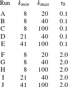
The flows we integrate are summarised in table 1. We consider flows with a range of spatial scales, with some (e.g. flows A and F) only having energy at large scales, some (e.g. flows E and J) only having energy at smaller scales and some (e.g. flows C and H) having energy at a wide range of spatial scales. In addition, some of the flows we consider are formed by adding together more restricted flows; for example, flow B is the sum of flows A and D (likewise
 $\text{G}=\text{F}+\text{I}$
), whilst flow H is the sum of flows B and E (likewise
 $\text{H}=\text{G}+\text{J}$
). These constructions will be used to examine whether the spatial scales act independently in generating the EMF. Furthermore, flows A–E are at short correlation time, whilst for flows F–J the correlation time of the eddies at scale
 $k$
is comparable to their turnover time at that scale. These flows are considered in the absence and presence of large-scale systematic shears of various strengths. Henceforth we utilise the shorthand notation
 $\text{Run}_{V_{0}}$
to represent the flow run in table 1, to which a shear of strength
 $V_{0}$
is added. For example,
 $\text{A}_{0}$
represents flow A from table 1 with no shear added, whilst
 $\text{F}_{20}$
represents flow F from table 1 to which a shear of
 $V_{0}=20$
is added.
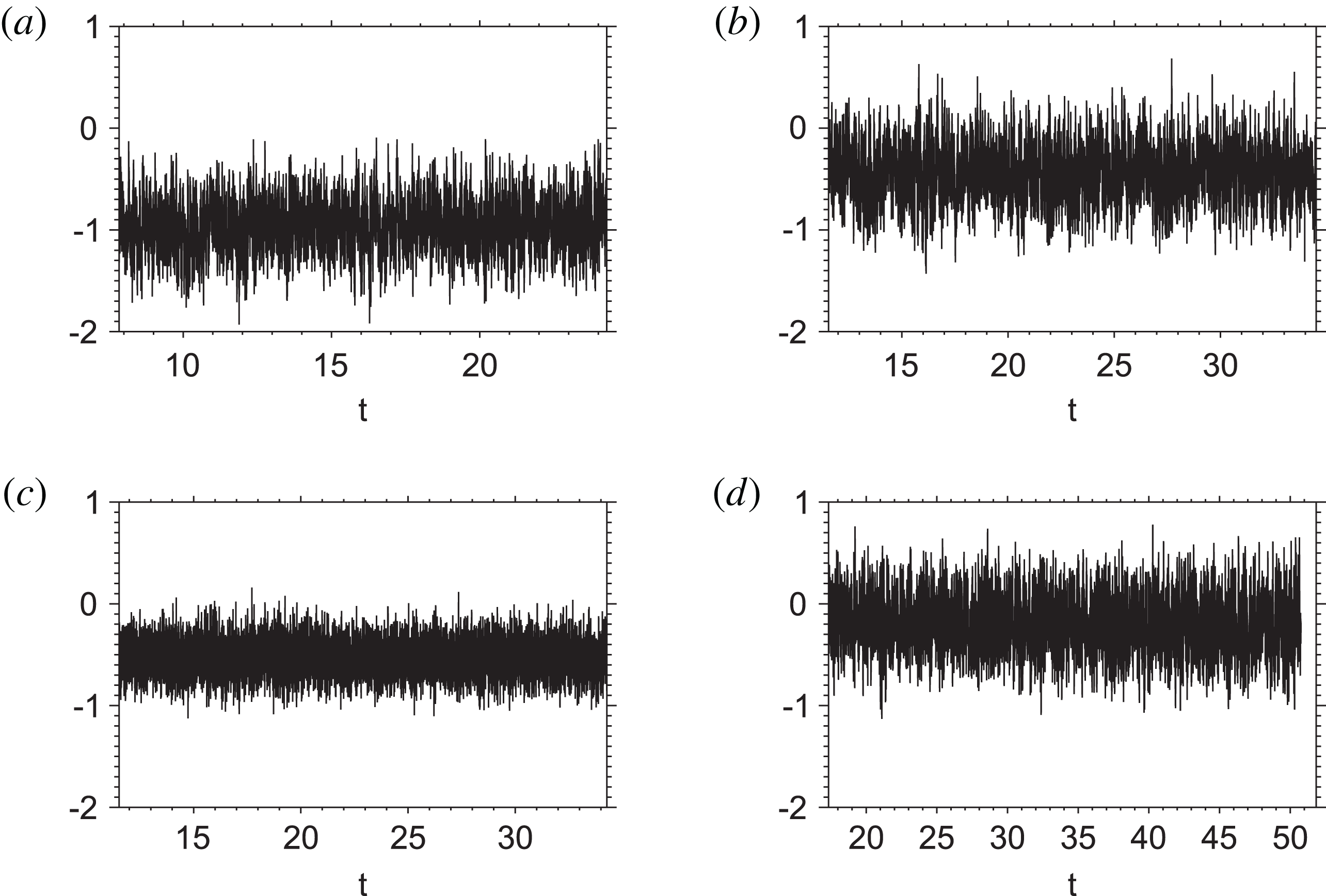
Time series of the EMF
 ${\mathcal{E}}$
for short-correlation-time flows with no shear. Here we consider flows: (a)
 $\text{C}_{0}$
, (b)
 $\text{B}_{0}$
, (c)
 $\text{E}_{0}$
and (d)
 $\text{A}_{0}$
.

The flows. All integrations are carried out with
 ${\it\eta}=10^{-4}$
.

Time series of the EMF
 ${\mathcal{E}}$
for moderate-correlation-time flows with no shear. Here we consider flows: (a)
 $\text{H}_{0}$
, (b)
 $\text{G}_{0}$
, (c)
 $\text{J}_{0}$
and (d)
 $\text{F}_{0}$
.

Figure 1 shows sample time series of the EMF for a range of short-correlation-time flows (with no imposed shear flow – so
 $V_{0}=0$
). The EMF is characterised by a well-defined mean with fluctuations about that mean that occur on a time scale comparable with the correlation time of the eddies. In figure 1(a) eddies on all scales from
 $k=8$
to
 $k=100$
contribute to the EMF; we note here that
 $\mathit{Rm}(8)\approx 500$
whilst
 $\mathit{Rm}(100)\approx 15$
for our choice of
 ${\it\eta}$
. In figure 1(b,c) the large and small scales contribute separately; we can compare the independence of the EMF generation at various scales by comparing the distributions for the EMF from the full spectrum to those calculated when the small and large scales are considered separately; this we do in the next subsection. It is also noticeable that the large-scale flows and small-scale flows have similar mean EMFs, but the range (and also variance) of the EMF from flows on the small scale is smaller. Thus the smaller scales are capable of contributing significant mean EMFs with tighter distributions than the large-scale flows. This will be quantified in § 3.3. Finally figure 1(d) shows the EMF for a case that only contains the very largest scales (
 $8\leqslant k\leqslant 20$
). These have a small mean and very large variance, a result that is in accord with arguments proposed above. Figure 2 shows that this behaviour persists for flows with moderate correlation times. Here the mean EMFs are larger than for the comparable flows with short correlation times, but the picture remains that smaller spatial scales are capable of contributing to the mean EMF without significantly affecting the variance. Recall here that the smaller scales are at smaller local magnetic Reynolds number
 $\mathit{Rm}(k)$
.
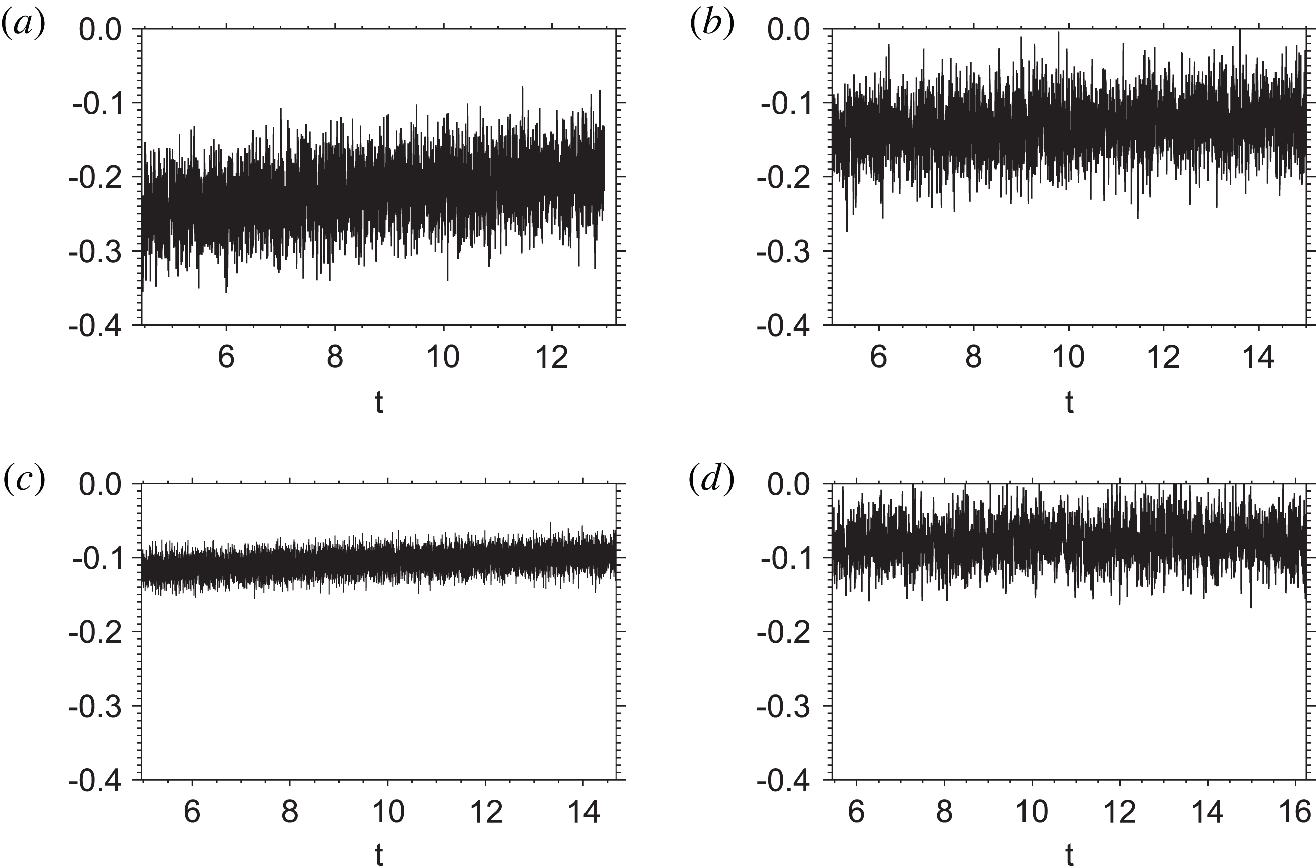
Time series of the EMF
 ${\mathcal{E}}$
for short-correlation-time flows with strong shear. Here we consider flows: (a)
 $\text{C}_{20}$
, (b)
 $\text{B}_{20}$
, (c)
 $\text{E}_{20}$
and (d)
 $\text{A}_{20}$
.

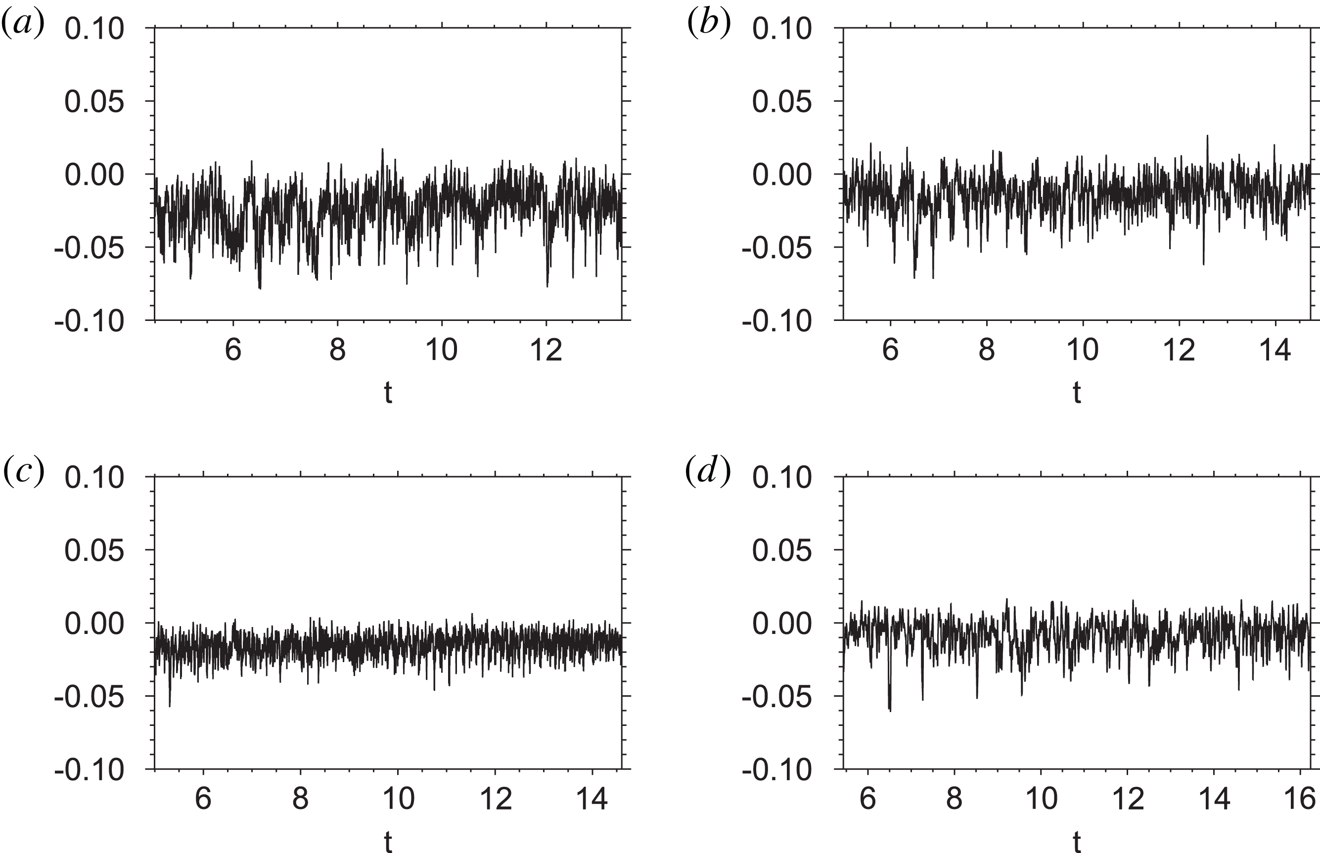
Time series of the EMF
 ${\mathcal{E}}$
for moderate-correlation-time flows with strong shear. Here we consider flows: (a)
 $\text{H}_{20}$
, (b)
 $\text{G}_{20}$
, (c)
 $\text{J}_{20}$
and (d)
 $\text{F}_{20}$
.

Figures 3 and 4 show the comparable time series for the cases when a strong shear is included for both short- and moderate-correlation-time flows. In all cases the shear has acted to reduce both the amplitude of the mean EMF and, perhaps more significantly, the fluctuations about that mean. Shear this strong is able to act to modify the EMF produced even by the flows on small scales. A quantification of this effect is included in § 3.3.
3.2. Contributions to the EMF from different scales and their independence
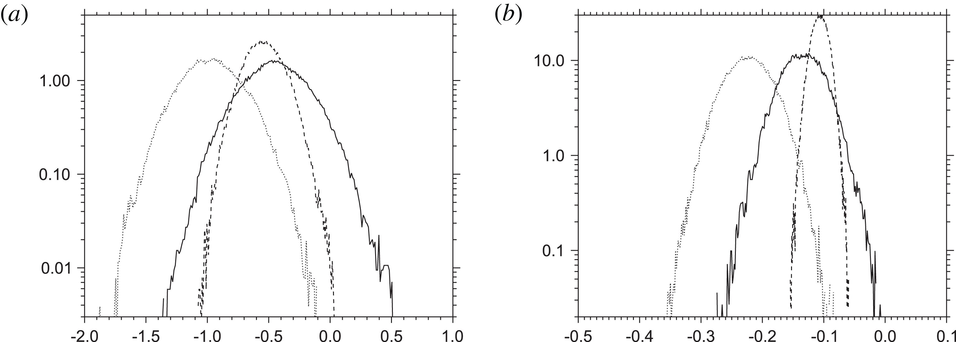
In this subsection we quantify the role of different scales in determining the EMF. In particular, we examine which scales are responsible for generating a significant mean EMF, and which lead to strong fluctuations about that mean. In order to be able to make such statements, it is necessary to determine the degree of independence of the different scales in the flow in their contribution to the flow. We achieve this by utilising the following procedure. We consider three flows: one comprises eddies at only large scales, one only at small scales, and one has both large- and small-scale components. We then determine the distributions of the EMF for these flows, which we term
 $\text{EMF}_{l}$
(the EMF for the large-scale flow)
 $\text{EMF}_{s}$
(the EMF for the small-scale flow) and
 $\text{EMF}_{a}$
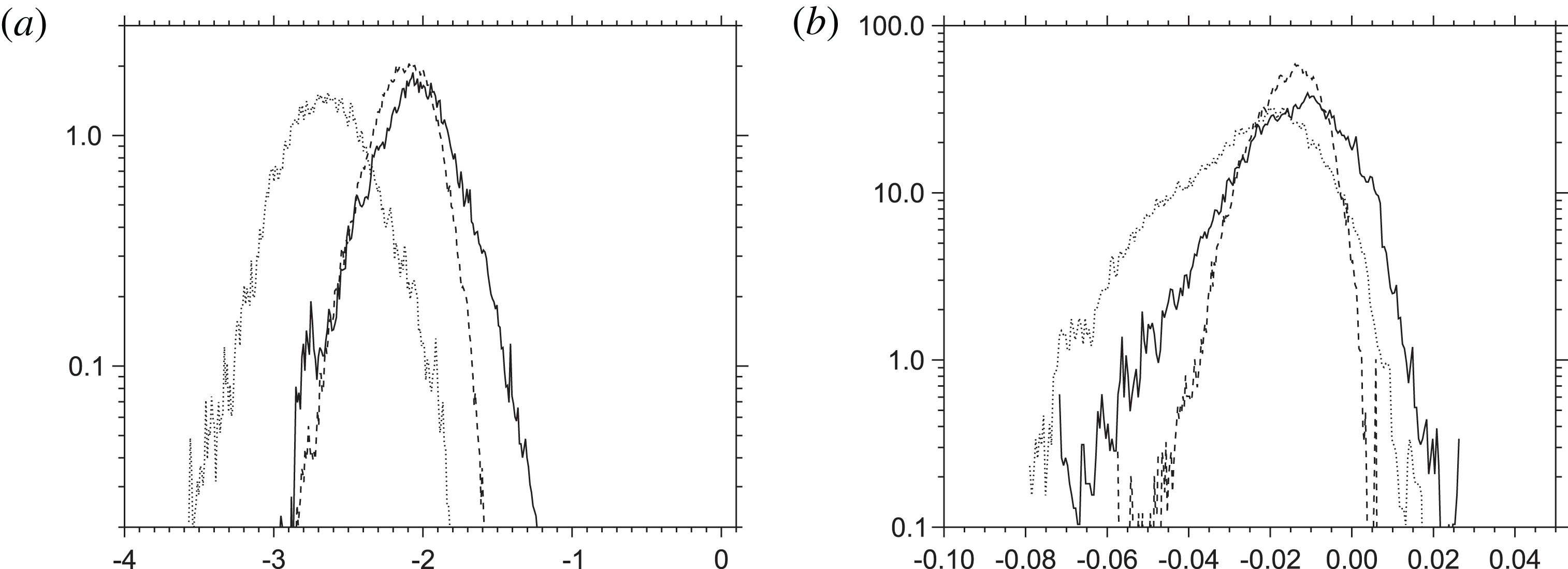
(the EMF for the flow with all components). These EMFs are shown in figure 5 for the short-correlation-time flow, in both the presence and absence of large-scale shear. A number of points may be made immediately. For these flows, it appears as though the large and small scales separately produce similar mean EMFs to each other. However, the fluctuations about this mean (as measured, say, by the variance of the distributions) are significantly larger for the flows at large scales than those at small scales. The flow that has energy at both large and small scales produces more mean EMF, but the variance of the EMF is dominated largely by fluctuations driven by the large scales (the variance does not differ significantly from that of the large-scale flow). The above statements are true in both the presence and absence of shear – the overall effect of the shear is in this case to reduce both the mean and the variance of the distributions for the EMF, as will be discussed in the next section. Figure 6 shows the corresponding distributions for the flows with longer correlation time. Here the striking feature is the significant effect of the shear flow on both the mean and variance of the EMF; the shear has had a significant effect in damping the EMF of all scales; we shall also see that the presence of a strong shear here has made the scales less independent.
Distributions of EMF at short correlation time for (a) cases with no shear
 $\text{B}_{0}$
(solid),
 $\text{E}_{0}$
(dashed) and
 $\text{C}_{0}$
(dotted) and (b) cases with strong shear
 $\text{B}_{20}$
(solid),
 $\text{E}_{20}$
(dashed) and
 $\text{C}_{20}$
(dotted).

Distributions of EMF at long correlation time for (a) cases with no shear
 $\text{G}_{0}$
(solid),
 $\text{J}_{0}$
(dashed) and
 $\text{H}_{0}$
(dotted) and (b) cases with strong shear
 $\text{G}_{20}$
(solid),
 $\text{J}_{20}$
(dashed) and
 $\text{H}_{20}$
(dotted).

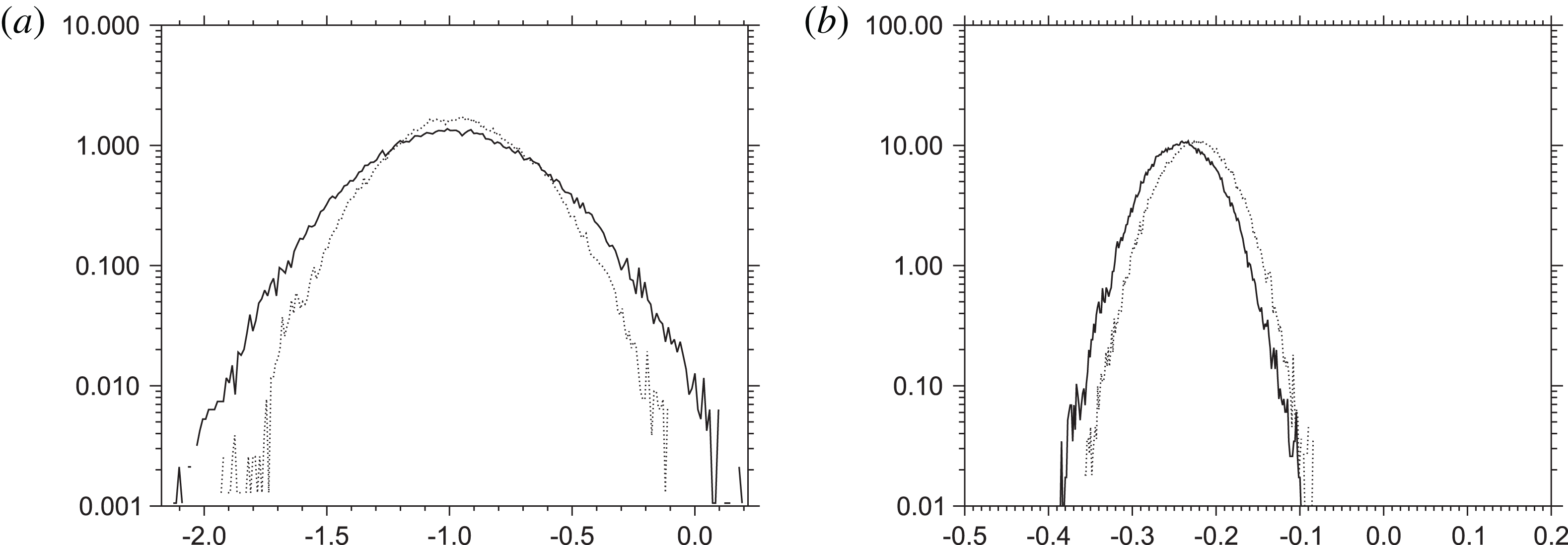
Distributions of the EMF for short-correlation-time flows: (a) cases
 $\text{C}_{0}$
(dotted) and
 $\text{E}_{0}+\text{B}_{0}$
(solid), and (b) cases
 $\text{C}_{20}$
(dotted) and
 $\text{E}_{20}+\text{B}_{20}$
(solid).

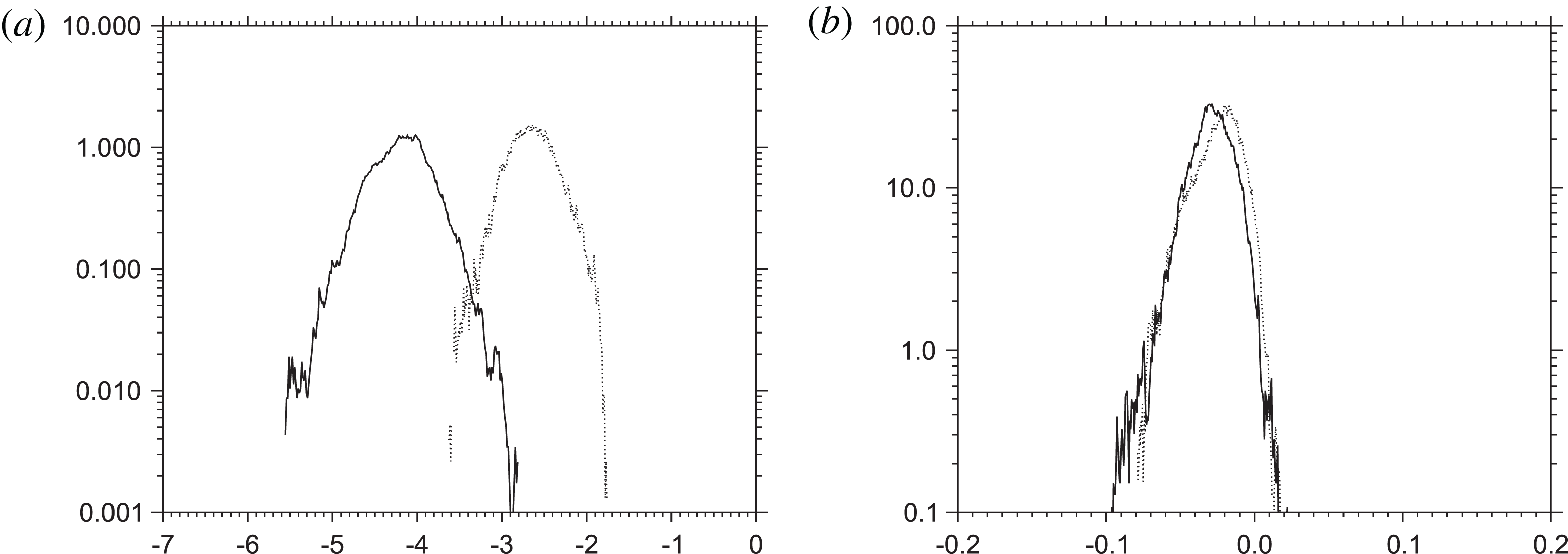
Distributions of the EMF for long-correlation-time flows: (a) cases
 $\text{H}_{0}$
(dotted) and
 $\text{J}_{0}+\text{G}_{0}$
(solid), and (b) cases
 $\text{H}_{20}$
(dotted) and
 $\text{J}_{20}+\text{G}_{20}$
(solid).

We proceed in calculating the independence of the scales, by examining the distribution
 $\text{EMF}_{a}$
and comparing it with the distribution of the variable that is the sum of the two EMFs (
 $\text{EMF}_{s}$
and
 $\text{EMF}_{l}$
).Footnote
3
If the large scales and small scales are acting independently, then these distributions should be the same. Figure 7 compares these distributions for the short-correlation-time flows. The distributions are extremely similar, both with and without shear, which suggests that for these flows the scales are contributing to the EMF independently – this is perhaps not surprising, owing to the rapid time scale on which the flows decorrelate (even at larger scales). The situation is similar in the presence of strong shear. However, for longer-correlation-time flows, in the absence of shear, the contributions to the EMF may not be independent, as shown in figure 8, which shows that the distributions are very different. This dependence is presumably a consequence of the larger scales, which have the longest correlation times, generating field that is acted on by the smaller scales. Interestingly, independence is re-established for these longer-correlation-time flows in the presence of strong shear, as shown in figure 8(b).
3.3. The role of shear, scaling of mean EMF and the fluctuations
It is clear from the considerations of the previous sections that, for flows with energy at large or small scales (or both large and small scales), the distribution of the EMF is a function of the applied mean shear. This appears to be true for both short-correlation-time flows and long-correlation-time flows. Here we quantify the dependence of the first two moments of the distribution on the mean imposed shear.
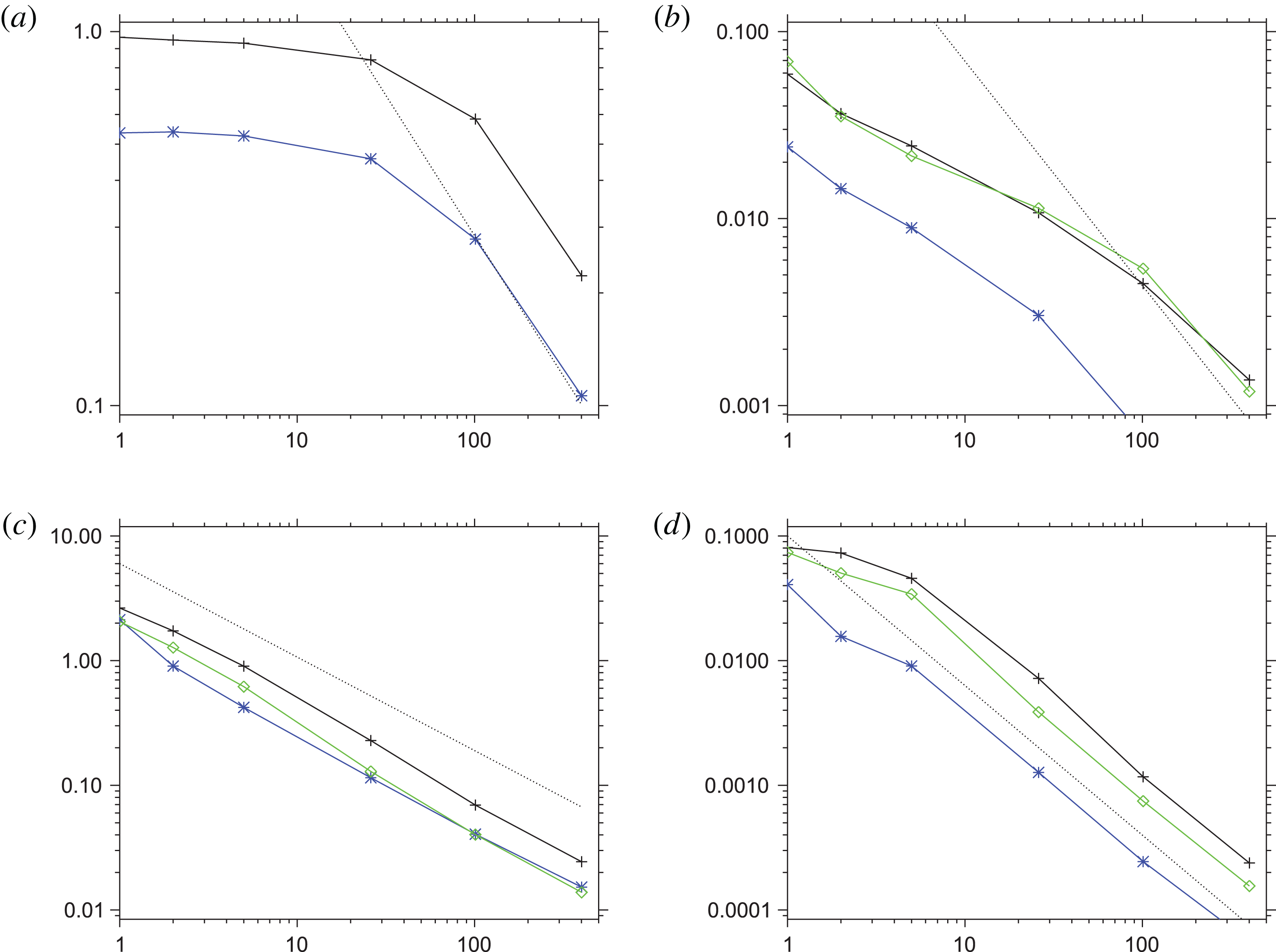
Figure 9 shows these moments as a function of
 $(1+V_{0}^{2})$
on a log–log plot. Figure 9(a,b) are for short-correlation-time flows. Figure 9(a) shows that, for these flows, the contribution to the mean EMF comes from both large and small scales for all values of the shear. For weak shears, the mean EMF is only weakly affected by the shear (with a slight decrease in the amplitude of the mean). At stronger shear rates, the mean is significantly reduced. In contrast, the variance is dominated by the large-scale flows (as noted earlier); the green curve tracks the black one closely. The effect of shear on the variance is more pronounced with an immediate decrease of the variance even for small shear rates. Thus for small shear rates, although the mean remains largely unaffected, the fluctuations about that mean are suppressed by the shear and the distribution of the EMF is narrowed.
Moments of EMF versus
 $(1+V_{0}^{2})$
. (a) Amplitude of the mean EMF for short-correlation-time flows for cases C (all scales; black), B (large scales; green) and E (small scales; blue). (b) Variance of EMF for the same cases. (c) Amplitude of the mean EMF for long-correlation-time flows for cases H (all scales; black), G (large scales; green) and J (small scales; blue). (d) Variance of EMF for the same cases.

For flows with longer correlation times (figure 9
a,b), there are some similarities and differences. Again there appears to be equal contributions to the mean EMF from the small- and large-scale flows, but in this case (and in contrast to the short-correlation-time flows) the shear does have a significant effect even for small
 $V_{0}$
. The variance of the EMF is again dominated by large-scale flows, and is again suppressed for even weak shears. Hence in this case both the mean EMF and the fluctuations about that mean are reduced.
We conclude this section by fitting the dependence of the moments on the shear rate. For small shear rates this is clearly a strong function of the correlation time of the flows, and so no universal fitting can be applied. We find that for large shears the scalings
 $$\begin{eqnarray}{\it\mu}_{\mathit{EMF}}\propto (1+V_{0}^{2})^{-{\it\lambda}}\quad \text{and}\quad {\it\sigma}_{\mathit{EMF}}^{2}\propto (1+V_{0}^{2})^{-{\it\kappa}}\end{eqnarray}$$
are consistent with the results for both long- and short-correlation-time flows, with
 ${\it\lambda}\approx 0.75$
and
 ${\it\kappa}\approx 1.2$
. The sensitivity of the variance to the strength of the shear is a key result, which can be used to interpret the dynamo’s tendency to suppress fluctuations in the presence of shear (as discussed in the conclusion below).
4. Conclusion
In this paper we have examined the generation of the EMF by multi-scale random flows. The EMF has a distribution with well-defined moments (such as mean and variance) that depend on the spatial scales contained in the flow and the strength of the systematic large-scale shear flow. We have shown that scales act more independently in generating the EMF in short-correlation-time flows than in long-correlation-time flows in the absence of shear. The presence of shear tends to make the scales act more independently for both short and long correlation times.
An important result is that the mean EMF and the fluctuations about that mean arise from different scales of the prescribed flow. Whereas all scales may contribute to the mean EMF, the large spatial scales consistently contribute more to the variance of the distribution. The role of shear in modifying the distribution of the EMF is also different for short- and long-correlation-time flows. For short-correlation-time flows, the mean EMF is only weakly dependent on shear rate; whilst for longer-correlation-time flows, the mean EMF is much more sensitive to the shear rate. We therefore believe that it is dangerous to extrapolate from short correlation times to long correlation times when considering the likely distributions of the EMF. We note that for both cases (long and short correlation times) the variance of the distribution of the EMF is sensitive to the strength of the shear.
We conclude by speculating on the importance of these results for large- and small-scale dynamo action. It is tempting to identify the mean EMF with a tendency of the resulting dynamo to produce large-scale fields, whereas fluctuations in the EMF about that mean may be identified with small-scale dynamos. If this is the case, then both large- and small-scale flows are able to contribute to the large-scale dynamo, large scales (which are at higher
 $\mathit{Rm}$
) contribute more to the small-scale dynamo. This is consistent with the theory proposed by Tobias & Cattaneo (Reference Tobias and Cattaneo2008a
). Moreover, the small-scale dynamo is more sensitive than the large-scale dynamo to the presence of shear. It is therefore plausible, as suggested by Tobias & Cattaneo (Reference Tobias and Cattaneo2013) and Cattaneo & Tobias (Reference Cattaneo and Tobias2014), that the primary effect of the presence of shear at high
 $\mathit{Rm}$
may be to suppress small-scale dynamo action whilst allowing the large-scale dynamo to manifest itself.
We conclude by discussing what is meant by a dynamo operating at high
 $\mathit{Rm}$
. Clearly, large
 $\mathit{Rm}$
can mean different things to different authors, and simply quoting a value of
 $\mathit{Rm}$
may be misleading. Two crucial values of
 $\mathit{Rm}$
can easily be identified in the kinematic regime. The first of these,
 $\mathit{Rm}_{c}$
, is the critical value of
 $\mathit{Rm}$
at which dynamo action sets in. The second,
 $\mathit{Rm}_{a}$
, is that value at which the growth rate of the flow approaches its asymptotic limit (for practical purposes this could be defined as coming within
 $5\,\%$
of this limit). Typically
 $\mathit{Rm}_{a}\gg \mathit{Rm}_{c}$
and is not usually accessible to three-dimensional calculations. Even for the Galloway–Proctor flow
 $\mathit{Rm}_{a}\approx 50\mathit{Rm}_{c}$
, and it is only the fact that the calculation is quasi-two-dimensional that allows access to magnetic Reynolds numbers greater than
 $\mathit{Rm}_{a}$
. We recognise that calculation of
 $\mathit{Rm}_{a}$
is difficult in fully three-dimensional calculations, but we argue here that it is incumbent on dynamo theorists to provide the value of
 ${\it\chi}=(\mathit{Rm}-\mathit{Rm}_{c})/\mathit{Rm}_{c}$
for their calculations so it is possible to evaluate whether their calculations may be close to asymptotic. Typically this value would need to be
 ${\it\chi}\sim O(100)$
before any claims of high
 $\mathit{Rm}$
should be made. We note that these calculations are performed with
 ${\it\chi}\sim 250$
and so can be regarded as being at high
 $\mathit{Rm}$
.
Acknowledgement
S.M.T. would like to thank STFC for funding.