





Impact Statement
High-fidelity datasets for deep learning surrogates in Fluid Mechanics are prohibitively expensive. We introduce a multi-fidelity training algorithm for autoencoders that relies on few high-fidelity samples enriched by many low-fidelity simulations to produce accurate surrogates (with quantified uncertainties) while reducing database construction cost by 20x.
1. Introduction
Fluid flow simulations for configurations of engineering interest remain computationally taxing when using high-fidelity approaches. For this reason, most of the current industrial applications rely on low-fidelity models (e.g., Reynolds-Averaged Navier–Stokes simulations—RANS), especially when many configurations need to be investigated (e.g., shape design optimization). However, in many cases of engineering interest, low-fidelity methods fail to provide accurate predictions, thus limiting the usefulness of the results.
Recent advances in Machine Learning (ML) have enabled data-driven surrogate models capable of accurately predicting aerodynamic performance in real time, greatly accelerating optimization processes. Nevertheless, in fields such as Fluid Mechanics, generating high-fidelity training datasets remains computationally expensive and time-consuming. In recent years, autoencoders (AEs) (Hinton and Salakhutdinov, Reference Hinton and Salakhutdinov2006) have become popular for the construction of reduced-order models. They are Deep Learning algorithms typically employed for dimensionality reduction and feature extraction. AEs can be viewed as a nonlinear extension of the Proper Orthogonal Decomposition (POD), reducing complex data into a low-dimensional compressed representation (latent space), with compression ratio much higher than that of POD (Milano and Koumoutsakos, Reference Milano and Koumoutsakos2002). The ability of AEs to make accurate predictions has been extensively discussed in recent literature, and many different approaches and architectures have been proposed (Agostini, Reference Agostini2020; Racca et al., Reference Racca, Doan and Magri2023; Solera-Rico et al., Reference Solera-Rico, Sanmiguel Vila, Gómez-López, Wang, Almashjary, Dawson and Vinuesa2024). Many articles discuss the problem of data collection for training AEs (and, in general, deep learning algorithms) in Fluid Dynamics. For instance, Tangsali et al. (Reference Tangsali, Krishnamurthy and Hasnain2020) showed that, in order to construct an AE capable of generalizing across many different flow regimes past an airfoil, a training database composed of thousands of simulations was required, which would be unfeasible for high-fidelity methods such as Large Eddy Simulations (LES). Training strategies that rely on a mixture of low- and high-fidelity results (multi-fidelity) have the potential to enable accurate deep learning approaches at a manageable computational cost.
Multi-fidelity applications for AEs remain an area with limited coverage in the literature. For instance, Shen et al. (Reference Shen, Patel, Xu and Alonso2024) proposed a multi-fidelity transfer learning method using AEs to efficiently construct a surrogate model for airfoil aerodynamics, employing Euler simulations (low fidelity) and RANS simulations on coarse grid (medium fidelity) and fine grid (high fidelity). In their approach, the objective is constructing a model capable of making high-fidelity predictions providing low-fidelity input. Partin et al. (Reference Partin, Geraci, Rushdi, Eldred and Schiavazzi2023) proposed a multi-fidelity network architecture composed of convolutional encoders, decoders, and skip connections, resulting in a model where different fidelities are learned simultaneously. In this case, sparse high-fidelity data are enriched with a large amount of low-fidelity data. They applied their method to classical benchmark problems: one-dimensional functional approximation and the solution of the pressure Poisson equation.
In the present article, we propose a method for constructing AE models able to provide high-fidelity predictions with quantified uncertainties at low computational cost (taking advantage of multi-fidelity methods) on a problem of practical engineering interest. Specifically, in the present article, we introduce a multi-branch AE to treat two-dimensional fields that are not spatially related but correspond to the same input parameters. Specifically, each dataset case comprises channels containing physical variables from different flow sections; we introduce a multi-fidelity training algorithm for AEs that enables a drastic reduction in the computational cost of database construction. The novelty of the multi-fidelity method lies in the fact that multi-fidelity papers in the literature typically refer to a coarse/fine solution of the same problem and introduce a relatively complex architecture that enables merging of the datasets. Here, the approach is general, that is, the data can be from completely different descriptions of the solution (including experiments, provided that the low-fidelity data are pre-processed to mimic the experimental data), and the data fusion is based on the idea of latent space enrichment. Finally, we applied an ensemble technique to provide predictions with quantified model uncertainties. The proposed method is applied to the prediction of jet flows exhausting from nozzles of different geometries. The multi-fidelity dataset is constructed using RANS simulations for the low-fidelity data and LES for the high-fidelity data.
Section 2 focuses on the comparison between RANS and LES solutions and experimental results available in the literature, highlighting the necessity of high-fidelity calculations. Section 3 describes the computational setup used for constructing the training database (Saetta et al., Reference Saetta, Massa, Tognaccini and Iaccarino2025) and the parametric description of the nozzle geometries. Section 4 is dedicated to describing the ML algorithms and methods employed for training a multi-fidelity AE and for making flow predictions with quantified uncertainties. In Section 5, the results of the trained model are discussed, first presenting a practical example of the encoding and decoding procedures, and then assessing the accuracy of the model predictions against CFD reference simulations.
2. Validation of flow simulations
The validation of the CFD simulations used to construct the database was carried out by comparing the numerical results with two available experiments: a hot round jet (Bridges and Wernet, Reference Bridges and Wernet2011) and a rectangular jet (Zaman, Reference Zaman2012).
2.1. Hot round jet
The open-source software SU2 (Economon et al., Reference Economon, Palacios, Copeland, Lukaczyk and Alonso2016), was used to perform RANS simulations, while the CharLES software (Goc et al., Reference Goc, Lehmkuhl, Park, Bose and Moin2021) was used for the Wall Modeled Large Eddy Simulations (WM-LES). Two computational grids were used for both RANS and LES to analyze the grid convergence. For RANS, the grids were taken from the NASA Turbulence Modeling Resource (https://turbmodels.larc.nasa.gov/jetsubsonichot_grids.html), and they had resolution of
$ 18\times {10}^3 $
 and
$ 72\times {10}^3 $
 cells. For the LES, the grids were generated using the CharLES grid generator and had resolution of
$ 11\times {10}^6 $
 and
$ 30\times {10}^6 $
 cells.
The nozzle exit Reynolds number, non-dimensionalized by the exit diameter, is
$ 6.15\times {10}^5 $
 , while the nozzle exit Mach number is
$ 0.376 $
 . The
$ k $
 –
$ \omega $
 SST turbulence model described by Menter (Reference Menter1994) was employed for the steady RANS simulations, while the subgrid model proposed by Vreman (Reference Vreman2004) was used for the LES. The computation of the statistics in the LES was performed after an initial transient of
$ \overline{t_{tr}}={t}_{tr}{U}_{id}/D=203 $
 over a simulation time of
$ \overline{t_{sim}}={t}_{sim}{U}_{id}/D=1354 $
 , with
$ \overline{\Delta t}=\Delta {tU}_{id}/D=6.77\times {10}^{-4} $
 , in which
$ {t}_{tr} $
 is the transient time,
$ {U}_{id} $
 is the jet velocity at the nozzle exit assuming fully expanded flow,
$ D $
 is the exit diameter,
$ {t}_{sim} $
 is the simulation time, and
$ \Delta t $
 is the simulation time step. The time step was chosen such that the simulation was carried out at
$ CFL\approx 2.0 $
 . A co-flow at
$ {M}_{\infty }=0.01 $
 was used outside the nozzle in both simulations.
The grid convergence and the comparison with the experiment of the mean streamwise velocity at the jet centerline are shown in Figure 1.
Grid convergence (left) and comparison with the experiment (right) of the mean streamwise velocity at the jet centerline by CharLES and SU2 for the hot round jet.

Figure 1. Long description
Two side-by-side line graphs with identical axes. The x-axis represents x all over D sub e q ranging from 0 to 20. The y-axis represents U all over U sub j ranging from 0.0 to 1.2.
Left Panel: Grid convergence study.
* The x-axis is x all over D sub e q.
* The y-axis is U all over U sub j.
* W M - L E S 11 times 10 super 6 (blue solid line) and W M - L E S 30 times 10 super 6 (black solid line) show nearly identical behavior, maintaining a plateau near 1.0 until x equals 5, then decaying asymptotically.
* R A N S 18 times 10 super 3 (blue dashed line) and R A N S 72 times 10 super 3 (black dashed line) maintain a plateau near 1.0 until x equals 8.5, followed by a sharper drop-off compared to the L E S models.
Right Panel: Comparison with experiment.
* W M - L E S (black solid line) follows the experimental data points (red dots) closely, showing a gradual decay starting at x equals 5.
* R A N S (blue solid line) maintains a plateau until x equals 8.5 before dropping, overestimating the velocity in the region between x equals 5 and x equals 10.
* Experimental data (red dots) shows the velocity decay beginning around x equals 4.
The RANS simulation significantly overpredicts the mean velocity near the nozzle exit, the region commonly referred to as the potential core. Meanwhile, across the entire axis, the LES show a more convincing agreement.
2.2. Rectangular jet
The capability of the LES to capture the flow features of rectangular jets was verified analyzing the jet with aspect ratio
$ AR=8 $
 studied by Zaman (Reference Zaman2012). For this analysis, only the LES were performed, with a grid generated using the CharLES grid generator composed of
$ \approx 30 $
 million cells. The nozzle exit Mach and Reynolds numbers were
$ 0.226 $
 and
$ 2.76\times {10}^5 $
 , respectively. In this analysis, statistics were computed after an initial transient of
$ \overline{t_{tr}}=96 $
 over a simulation time of
$ \overline{t_{sim}}=640 $
 , with a time step of
$ \overline{\Delta t}=3.20\times {10}^{-4} $
 , where
$ {D}_{eq} $
 is the nozzle exit equivalent diameter. The mean streamwise velocity at the jet centerline, as obtained by the LES and the experiment, is shown in Figure 2.
Comparison of the mean streamwise velocity at the jet centerline obtained by the CharLES and the experiment for the rectangular jet.

Figure 2. Long description
The line graph features a horizontal X-axis labeled x forward slash D sub e q ranging from 0.0 to 20.0 and a vertical Y-axis labeled U forward slash U sub j ranging from 0.0 to 1.2.
Two data series are presented:
* CharLES is represented by a solid black line.
* Experimental data is represented by red circular dots.
From x forward slash D sub e q equals 0 to approximately 2, both datasets show a plateau where the velocity ratio remains constant at 1.0.
Between x forward slash D sub e q equals 2 and 10, there is a steep non-linear decrease in velocity. The CharLES simulation and experimental dots show high agreement in this region, following an identical downward curve.
From x forward slash D sub e q equals 10 to 20, the velocity continues to decrease at a slower, asymptotic rate. In this region, a slight divergence occurs where the CharLES black line remains marginally higher than the red experimental dots, which end at approximately x forward slash D sub e q equals 17.5.
The agreement with the experiment further validated the LES methodology. Due to the highlighted limitations of the RANS model in capturing the jet potential core, in the following RANS will be referred to as low fidelity (LF), while LES will be referred to as high fidelity (HF).
3. Nozzle jet database
3.1. Parametric description
The adopted reference system is shown in Figure 3 for a sample nozzle.
A sample of nozzle database.

The nozzle cross-section is described by a superellipse (Davis and Gessner, Reference Davis and Gessner1992). A database of nozzles (described in more detail in Section 5.1) was generated based on the following geometric design parameters:
-
• $ {f}_A^{\ast } $
 : cross-section area distribution. A low
$ {f}_A^{\ast } $
indicates that area variations are concentrated near the nozzle inlet, whereas a high
$ {f}_A^{\ast } $
indicates that area variations are concentrated near the nozzle exit.
-
• $ {AR}_{out} $
: exit aspect ratio (width over height). -
• $ {n}_{out} $
: exit superellipse factor. With
$ {n}_{out}=2 $
, the exit is an ellipse, while increasing
$ {n}_{out} $
makes it progressively more rectangular.


All nozzles maintain a circular inlet with the same area, while also keeping the same length
$ L $
 and outlet area. The analytical laws used to define the geometry are omitted for the sake of brevity. The influence of the parameters on the nozzle shape is shown in Figure 4.
Isometric view and section at
$ x/L=-0.5 $
 of sample geometries at different
$ {f}_A^{\ast } $
 (top),
$ {AR}_{out} $
 (middle), and
$ {n}_{out} $
 (bottom).

Figure 4. Long description
The grid is divided into three rows, each varying a specific parameter while holding others constant.
Top Row: Varies f sub A super asterisk with A R sub out equals 5 and n sub out equals 30.
* Left panel: f sub A super asterisk equals 0.50. The conduit tapers inward toward the center.
* Middle panel: f sub A super asterisk equals 1.00. The conduit maintains a more uniform transition.
* Right panel: f sub A super asterisk equals 1.50. The conduit bulges outward in the middle section.
All three panels show a rounded rectangular cross-section.
Middle Row: Varies A R sub out with f sub A super asterisk equals 1.00 and n sub out equals 30.
* Left panel: A R sub out equals 1. The cross-section is a rounded square.
* Middle panel: A R sub out equals 5. The cross-section is a wide rounded rectangle.
* Right panel: A R sub out equals 10. The cross-section is a very thin, elongated rounded rectangle.
Bottom Row: Varies n sub out with f sub A super asterisk equals 1.00 and A R sub out equals 5.
* Left panel: n sub out equals 2. The cross-section is a perfect ellipse.
* Middle panel: n sub out equals 5. The cross-section is a rectangle with heavily rounded corners.
* Right panel: n sub out equals 50. The cross-section is a sharp-edged rectangle with almost no corner rounding.
In all isometric views, the transition begins from a circular inlet on the left and evolves into the specified cross-sectional shape on the right.
3.2. Computational setup
Turbulence is deeply affected by nozzle geometric variations, because the jet exit velocity distribution determines the initial condition of the jet shear layers and its subsequent mixing. In addition, specific turbulence modeling choices (RANS vs. LES) induce differences in the results, with the RANS models being unable to represent the critical physical processes. RANS simulations fail to capture the generation of secondary flows in rectangular nozzles, which arise from the anisotropy of Reynolds stress (Bradshaw, Reference Bradshaw1987). Moreover, the breakdown of the coherent structures occurring in the jet can not be accurately captured by the present steady RANS model. On the other hand, LES can accurately capture stress-induced secondary flows and the instantaneous behavior of the coherent structures, and is therefore referred to as a high-fidelity physical representation of the nozzle jet flow. The LES resolve the instantaneous flow field, which is not symmetric even in a geometrically symmetric configuration. Meanwhile, the RANS equations solve the statistically averaged flow field, and the mean flow is symmetric under symmetric geometry and boundary conditions. Therefore, the flow resolved in the RANS simulation was defined on a quarter of the domain, while the flow resolved in the LES was defined as the full
$ 360 $
 degree field. In both cases, the highest refinement is near the walls and inside the jet shear layer.
The computational grids used for the RANS simulations were generated by an automatic multi-block structured grid generator developed in-house, while the grids used for the LES were generated following the same methodology used for the hot round jet and rectangular jet. A grid convergence analysis was carried out for both low- and high-fidelity simulations on a sample geometry (
$ {f}_A^{\ast }=1.00 $
 ,
$ {AR}_{out}=10 $
 ,
$ {n}_{out}=30 $
 ), ensuring no influence of the grid resolution on the nozzle jet physics. The grid resolutions were
$ \approx 700\times {10}^3 $
 (fine) and
$ \approx 260\times {10}^3 $
 (coarse) for RANS, and
$ \approx 40\times {10}^6 $
 (fine) and
$ \approx 8\times {10}^6 $
 cells (coarse) for LES. Figure 5 shows the fine grids, and Figure 6 shows the streamwise velocity along the jet centerline for both low and high fidelity. The results were nearly equal, and the fine grids were chosen for both fidelities due to the higher quality of the flow field.
Fine computational grid used for RANS (left) and LES (right) for the geometry
$ {f}_A^{\ast }=1.00 $
 ,
$ {AR}_{out}=10 $
 ,
$ {n}_{out}=30 $
 .

Figure 5. Long description
The figure consists of two side-by-side panels showing different mesh resolutions for fluid dynamics simulations.
* Left Panel (R A N S): A structured computational grid for Reynolds-Averaged Navier-Stokes simulations. The grid is divided into vertical colored blocks (cyan, purple, green, blue, and yellow) that follow the curvature of a nozzle wall. The mesh lines are visible, showing a coarser resolution compared to the right panel. The grid lines curve upward and then flatten out as they move from left to right, following the expanding geometry of the nozzle.
* Right Panel (L E S): A much finer, high-density mesh used for Large Eddy Simulations. The central region of the nozzle is filled with a dense, grey, uniform grid that appears almost solid due to the high cell count. Along the top and bottom curved walls, there is a distinct dark black band indicating extremely high mesh refinement at the boundary layers to capture near-wall turbulence. The background outside the nozzle geometry is a solid tan color.
Streamwise velocity along the jet centerline of coarse and fine grid for RANS (left) and LES (right) for the geometry
$ {f}_A^{\ast }=1.00 $
 ,
$ {AR}_{out}=10 $
 ,
$ {n}_{out}=30 $
 .

Figure 6. Long description
A two-panel line graph. Both panels share the same axes: the x-axis is x forward slash D sub e q ranging from 0.0 to 20.0, and the y-axis is U forward slash U sub j ranging from 0.2 to 1.0. Each graph contains a black line for coarse grid and a red line for fine grid.
* Left Panel (R A N S): Both lines start at a plateau of 1.0 until x forward slash D sub e q equals 2.5. After this point, they show a smooth asymptotic decay. The black coarse line remains slightly above the red fine line throughout the decay until they converge at 0.2 near the end of the axis.
* Right Panel (L E S): The lines show a plateau at 1.0 until approximately x forward slash D sub e q equals 1.5. The subsequent decay is more rapid and slightly more irregular compared to the left panel. The red fine line and black coarse line are closely intertwined, with the red line showing slightly higher velocity between x forward slash D sub e q values of 2.5 and 7.5 before converging with the black line for the remainder of the plot.
The nozzle inlet total pressure and temperature were set to
$ {p}_0/{p}_{\infty }=1.79 $
 and
$ {T}_0/{T}_{\infty }=2.69 $
 where
$ {p}_{\infty } $
 and
$ {T}_{\infty } $
 denote the ambient pressure and temperature. The nozzle exit Mach number is
$ 0.953 $
 , and the nozzle exit Reynolds number, non-dimensionalized using the equivalent diameter, is
$ 6.44\times {10}^6 $
 . For each simulation, the following global metrics were computed:
-
• Potential core length $ {L}_{pc} $
. -
• Half-jet spreading $ {y}_{1/2} $
and
$ {z}_{1/2} $
at
$ x/{D}_{eq}=2 $
.


In the present application, the database is composed of tensors obtained by interpolating the CFD data onto structured Cartesian grids. The channel groups are:
-
1. $ {\mathbf{b}}_1 $
:
$ x $
,
$ z $
grid coordinates,
$ {U}_x $
,
$ {U}_z $
velocity components in the
$ x-z $
plane at
$ y/{D}_{eq}=0 $
. The structured grid extended in
$ x\in \left[-L,20{D}_{eq}\right] $
in the streamwise direction, while up to the half-width coordinate (see Mi et al., Reference Mi, Deo and Nathan2005) in the spanwise direction. -
2. $ {\mathbf{b}}_2 $
:
$ y $
,
$ z $
grid coordinates,
$ {U}_x $
,
$ {U}_z $
velocity components in the
$ y-z $
plane at
$ x/{D}_{eq}=1 $
. The grid was rectangular in the transverse direction and was extended from the jet half-widths coordinates of the minor half-width in both directions. -
3. $ {\mathbf{b}}_3 $
:
$ y $
,
$ z $
grid coordinates,
$ {U}_x $
,
$ {U}_z $
velocity components in the
$ y-z $
plane at
$ x/{D}_{eq}=2 $
. The grid definition methodology was the same as the one for
$ x/{D}_{eq}=1 $
.





A jet flow for a sample nozzle used as input to the AE is shown in Figure 7.
Contour map of streamwise velocity for a sample nozzle.

Figure 7. Long description
The visualization begins at the left with a transparent, tapered nozzle housing a central horizontal plane. Inside the nozzle, velocity contours transition from light blue at the inlet to yellow and red toward the exit.
As the flow exits the nozzle, it passes through two vertical cross-sectional planes. These planes show a high-velocity red core surrounded by a thin yellow transition layer and a dark blue outer boundary.
Downstream of the nozzle, a long horizontal slice represents the exhaust plume. The velocity is highest (dark red) immediately after the exit and gradually dissipates, transitioning through orange, yellow, and light blue, eventually becoming dark blue at the far right.
A coordinate triad at the bottom center defines the orientation. The y-axis points upward, the x-axis points to the right along the flow direction, and the z-axis points toward the viewer.
The RANS simulations were carried out using Intel Xeon Gold 6230R processors, with a mean time-to-solution of approximately 7 hours on 16 CPUs. The LES simulations were performed using A100 GPUs on the GPU-accelerated partition of Leonardo’s exascale system for HPC and AI applications (Turisini et al., Reference Turisini, Amati and Cestari2023). Flow statistics were computed after an initial transient of
$ \overline{t_{tr}}=200 $
 over
$ \overline{t_{sim}}=100 $
 , with a time step of
$ \overline{\Delta t}=1.00\times {10}^{-3} $
 , resulting in a mean time-to-solution of approximately 3 hours on 16 GPUs. While we acknowledge that this simulation time is not sufficient to reach full statistical convergence, this choice will be justified in Section 5.3.
The computational cost per simulation for RANS (LF) and LES (HF) is shown in Table 1. The computational cost of a fully statistically converged LES, with
$ \overline{t_{sim}}=2000 $
 , is also reported. The RANS simulations were carried out on 16 CPUs, while the LES on 16 GPUs.
Computational cost of single low- and high-fidelity simulations

Table 1. Long description
The table consists of three columns: Fidelity Type, Device, and Cost.
* The first row shows L F simulations using a C P U Intel Xeon Gold 6230R at a cost of 122 C P U h.
* The second row shows H F simulations with t sub sim bar equal to 100 using a G P U NVIDIA A100 at a cost of 45.7 G P U h.
* The third row shows H F simulations with t sub sim bar equal to 2000 using a G P U NVIDIA A100 at a cost of 335 G P U h.
3.3. Impact of geometry variation
Many authors have analyzed the effects of geometry on jet flows, including Tsuchiya et al. (Reference Tsuchiya, Horikoshi and Sato1986), Mi and Nathan (Reference Mi and Nathan2009), Zaman (Reference Zaman2012). The results found in the present work are consistent with those reported in the literature. However, it is important to consider the impact of the geometrical parameters in the underlying physics, which is briefly discussed here. Figure 8 shows the variation of the streamwise velocity fields with respect to the input parameters. Each parameter affects different zones of the flow field: the cross-section area distribution affects the flow field inside the nozzle; the aspect ratio mostly impacts the jet; and the superellipse factor influences the transverse cross-section of the jet. The distribution of the cross-section area influences the location of higher gradients in the nozzle, thereby impacting the thrust, back pressure, and flow development. The exit aspect ratio significantly affects the jet flow field, with the velocity decaying faster at higher aspect ratios due to the stronger coherent structures forming at the nozzle exit. Finally, the superellipse factor induces different velocity profiles in the jet cross-section, with the profile being more rounded at lower superellipse factors. This effect tends to disappear further away from the nozzle exit due to the stronger influence of the jet shear layers and turbulent mixing (Zaman, Reference Zaman1996). Although the aspect ratio is the most dominant parameter in the underlying physics, variations in the cross-section area distribution and the superellipse factor induce changes in the flow field significant in design optimization studies. Therefore, the ability of the AE to capture both large-scale and subtle variations in the underlying physics represents a significant advantage.
Effects of cross-section area distribution (left), aspect ratio (middle), and superellipse factor (right) on the flow field. The black lines denote the nozzle exit.

Figure 8. Long description
The figure consists of three columns of contour plots, each with three rows. All plots use a color scale for U all over U sub j ranging from 0.2 in blue to 1.0 in red.
Left Column: Cross-section area distribution f super star sub A.
- Top: f super star sub A equals 0.5 shows a gradual expansion with a large red high-velocity core.
- Middle: f super star sub A equals 1.0 shows a more rapid expansion.
- Bottom: f super star sub A equals 1.5 shows a bulging nozzle profile with a concentrated high-velocity core.
Middle Column: Aspect ratio A R sub out.
- Top: A R sub out equals 1.0 shows a narrow, elongated red core that tapers quickly into blue.
- Middle: A R sub out equals 5.0 shows a wider red core that persists further downstream.
- Bottom: A R sub out equals 10.0 shows the widest red core and a broader plume expansion.
Right Column: Superellipse factor n sub out.
- Top: n sub out equals 5.0 shows a rounded, elliptical velocity cross-section.
- Middle: n sub out equals 10.0 shows a more rectangular cross-section with rounded corners.
- Bottom: n sub out equals 30.0 shows a nearly perfect rectangular velocity profile.
In the first two columns, a vertical black line marks the nozzle exit, separating the internal flow from the external plume.
4. The Machine Learning algorithm
The ML algorithm employed combines AE architectures and training methods for multi-fidelity predictions with quantified uncertainties. Specifically, an AE baseline architecture is introduced (the Multi-Branch Autoencoder—MBA). This AE is then trained using a multi-fidelity algorithm for AEs (AutoEncoder with Sequential Training and Adaptive Resolution—AESTAR); finally, an ensemble of trained AEs is constructed to provide predictions with quantified uncertainties. The three algorithms are briefly described below.
4.1. Autoencoder baseline: multi-branch autoencoder
The proposed AE has a multi-branch structure and will be denoted as MBA. Due to the use of convolutional layers, the dataset must be converted first to a tensor of shape
$ N\times C\times I\times J $
 (cases
$ \times $
 channels
$ \times $
 $ i $
 -grid elements
$ \times $
 $ j $
 -grid elements). The channels of the training dataset are the
$ {U}_x $
 and
$ {U}_z $
 velocity components in different planes:
$ x $
 -
$ z $
 plane and
$ y $
 -
$ z $
 planes. Because the channels belonging to different planes contain information that is not spatially related, a multi-branch structure is required. However, they share the same global information about the design parameters of the dataset. For this reason, multiple convolutional branches are considered, all merging in a shared latent vector. Figure 9 describes the multi-branch architecture proposed here. In the figure, each tensor (case) in the database can be divided into three groups of channels (green, blue, and red)
$ \mathbf{x}=\left[{\mathbf{b}}_1,{\mathbf{b}}_2,{\mathbf{b}}_3\right] $
 . Each channel group is passed through a different encoder function obtaining three latent vectors:
$ {\overline{\mathbf{V}}}_i={\mathbf{e}}_i\left({\mathbf{b}}_i\right) $
 . The latent vectors coming from different branches are projected into one shared latent vector
$ \mathbf{V} $
 (in purple) using a fully connected network. The projected latent space is shared across different decoders to reconstruct the input tensor:
$ \hat{{\mathbf{b}}_i}={\mathbf{d}}_i\left(\mathbf{V}\right) $
 .
Schematic representation of the Multi-Branch Autoencoder (MBA) architecture.

Figure 9. Long description
The flowchart begins on the far left with an input vector x consisting of components b sub 1, b sub 2, and b sub 3, represented by a 3D cube with red, blue, and green segments. Arrows lead from these segments into three parallel encoder branches labeled e sub 1 (red), e sub 2 (blue), and e sub 3 (green). Each encoder consists of four progressively smaller rectangular blocks followed by a triangular cluster of dots and a final small vertical bar labeled V-bar sub 1, V-bar sub 2, and V-bar sub 3 respectively. These three outputs converge into a single vertical multi-colored bar, which passes through a gray trapezoidal bottleneck into a central purple bar labeled V. From this central point, purple arrows branch out into three parallel decoder paths labeled d sub 1, d sub 2, and d sub 3. Each decoder mirrors the encoder structure in reverse, starting with a small vertical bar, a triangular dot cluster, and four progressively larger rectangular blocks. The outputs of these three branches converge on the far right into a second 3D cube with red, blue, and green segments, representing the reconstructed output vector x-hat with components b-hat sub 1, b-hat sub 2, and b-hat sub 3.
4.2. The multi-fidelity training algorithm
For the treatment of multi-fidelity databases composed of simulations obtained with different physical models (e.g., Euler, RANS, DES, LES, etc.), we introduce the algorithm called AESTAR. It is a training algorithm for AEs naturally suited for multi-fidelity databases, based on a sequential training of AEs and an unsupervised conditioning of the latent space to construct successive latent representations. In the literature, latent space conditioning is typically achieved by introducing an additional term in the loss function, designed to enforce specific constraints on the latent variables. In other words, it guides the latent space toward a desired topological structure. Li et al. (Reference Li, Zhang and Chen2022) introduced a physics-based conditioning of the latent space, while a specific geometrical topology was enforced in An and Jeon (Reference An and Jeon2024). This practice introduces additional information (bias) into the latent space during training. In contrast, the conditioning method proposed in the present work leverages knowledge extracted from the preceding training steps, and therefore operates without any a priori bias. The conditioning involves only the latent subspaces of the current and previous training instances. Consequently, the algorithm can be regarded as an unsupervised latent space conditioning technique.
The algorithm scheme is reported in Figure 10.
$ {D}^{(1)} $
 and
$ {D}^{(2)} $
 are, respectively, low- and high-fidelity databases. First, an AE
$ {}^1 $
 with a latent space dimension of
$ p $
 is trained on
$ {D}^{(1)} $
 . Then, in a second step, another AE
$ {}^2 $
 is trained with a database composed by
$ {D}^{(1)}\cup {D}^{(2)} $
 and a latent space dimension of
$ P>p $
 . In the first step, the loss function is defined solely as the error between the input and its reconstruction. In the second step, the latent space conditioning term (
$ C\left(\mathbf{V}\right) $
 ) is added, thus the loss function employed becomes:
Schematic representation of the training and architecture of the AESTAR algorithm for adaptive resolution databases.

Figure 10. Long description
The diagram consists of two vertically stacked rows representing sequential training stages.
Top Row: A E super 1
* Input: A single green cube labeled D super 1.
* Process: A black arrow points to an encoder-decoder structure. It begins with a tall blue vertical bar, followed by three green bars of decreasing height.
* Bottleneck: A cluster of green dots tapers into a small red rectangle labeled with a red p.
* Output: The structure mirrors the encoder with three increasing green bars and a final tan bar. The entire row is labeled A E super 1 on the right.
Bottom Row: A E super 2
* Input: Two cubes, one green labeled D super 1 and one blue labeled D super 2.
* Process: A black arrow points to a similar encoder-decoder structure.
* Conditioning: A blue vertical arrow labeled p conditioning descends from the red p in the top row to the bottleneck of the second row.
* Bottleneck: The bottleneck in this row is a split blue and red rectangle. Below it is a red P and a blue dotted arrow pointing downward to three dots, indicating further iterations.
* Output: The structure ends with a tan bar and is labeled A E super 2 on the right.

where
$ \mathrm{\mathcal{L}}\left(\mathbf{x},\hat{\boldsymbol{x}}\right) $
 is the loss term relative to the reconstruction error,
$ x $
 and
$ \hat{x} $
 are the input data and its reconstruction,
$ \mathbf{V} $
 is the latent vector, and
$ \delta $
 is a weight introduced to balance the relative importance between the two terms in the loss function.
$ C\left(\boldsymbol{V}\right) $
 is the latent space conditioning term:

where
$ I $
 denotes the training step,
$ {V}_i $
 is the
$ i $
 -th latent variable, and
$ p $
 is the number of latent variables up to the
$ I $
 -th training step. The distinction between the formulations for databases
$ {D}^{(I)} $
 and
$ {D}^{\left(I-1\right)} $
 arise from the fact that the additional latent variables are left free to be learned in the higher-fidelity cases, whereas they are conditioned to zero for the lower-fidelity ones. This preserves consistency with the latent space identified at the previous fidelity level, where such additional latent variables were absent. In the present work,
$ \mathrm{\mathcal{L}}\left(\mathbf{x},\hat{\mathbf{x}}\right) $
 is

where
$ N $
 is the number of elements over which the loss is evaluated, the first term is the Mean Squared Error,
$ \nabla $
 is the 2D discrete gradient, and
$ {\nabla}^2 $
 is the 2D discrete Laplacian. The former computed using convolutions with kernels
$ {G}_x=\left[-1\hskip0.5em 1\right] $
 along the width and
$ {G}_y=\left[\begin{array}{c}-1\\ {}1\end{array}\right] $
 along the height; and the latter using the kernel
$ L=\left[\begin{array}{ccc}0& 1& 0\\ {}1& -4& 1\\ {}0& 1& 0\end{array}\right] $
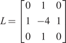 . The coefficients
$ {a}_i $
 are hyper-parameters that weight the relative importance of the loss terms. The spatial regularization terms are based solely on the pixel representation of the fields. Meaning that, during training, the first and second derivatives are not computed in the physical space (
$ x $
 and
$ y $
 coordinates), but in the pixel space. For this reason, these terms can be used for any channel in the input data, even when information about spatial coordinates is unavailable. In our experiments, predictions exhibit some non-physical oscillations when using only the MSE. While both MSE and MSE + regularization losses capture the overall behavior, those computed using only the MSE are noisy.
This composition of the loss function, with spatial regularization terms, is inspired by other works in literature which employ gradient and Laplacian loss terms for enhance super-resolution techniques in convolutional neural networks (Mathieu et al., Reference Mathieu, Couprie and LeCun2016; Lin et al., Reference Lin, Zhang, Yang, Cruz, Zhang and Gao2024).
This algorithm is motivated by the fact that, in fields such as Fluid Mechanics, the construction of high-fidelity databases can be computationally prohibitive. For this reason, we introduced the present algorithm to train a surrogate model capable of delivering high-fidelity predictions by exploiting multi-fidelity datasets composed of many low-fidelity (inexpensive) and few high-fidelity (expensive) simulations. In the first training step, an initial AE is built to predict low-fidelity data. The second step is aimed at learning a correction term that maps low-fidelity information to high-fidelity data within the latent space. This stage is performed by initializing the AE weights with those learned in the previous step. The conditioning term then establishes a soft correspondence between low- and high-fidelity data associated with the same parameters.
Each successive phase of training can rely on a dataset with progressively higher-fidelity data. The resulting algorithm provides adaptive resolution, in the sense that the same trained AE can return reconstructions selectively associated with a specific fidelity level. Furthermore, the sequential increase in latent space dimension introduces information that can be directly attributed to the increased fidelity of the dataset. Beyond multi-fidelity training, the proposed procedure also enables the construction of datasets that sequentially incorporate additional physical processes, while clearly separating the contribution of each subset. For linear problems, this is analogous to a superposition principle. Since the AESTAR algorithm is a training strategy rather than an architecture, it can be naturally applied to any AE architecture.
4.3. Predictions with quantified uncertainties
To assess the confidence in the multi-fidelity AE predictions we use an ensemble technique, by constructing an ensemble of AEs and computing mean and standard deviation of their predictions (Saetta et al., Reference Saetta, Tognaccini and Iaccarino2024). In the present work, an ensemble of multi-fidelity MBAs is constructed. Following the guidelines of the previous article of Saetta et al. (Reference Saetta, Tognaccini and Iaccarino2024), each model in the ensemble has randomly initialized trainable parameters, different AE’s architectures (varying kernel sizes, kernel strides, number of convolutions, dropout probability, number of trainable parameters) and different random selection of subsets for training and validation sets. In this work, only model-form uncertainty is taken into account. Figure 11 shows a schematic representation of how the method works when using the decoder as generative network: latent variables are provided as input to an ensemble of
$ N $
 trained decoders, whose
$ N $
 outputs are averaged to compute the mean and the standard deviation of the predictions. Details of this method can be found in Saetta et al. (Reference Saetta, Tognaccini and Iaccarino2024).
Schematic representation of the ensemble technique of AE predictions for the quantification of model uncertainties.

5. Nozzle jet flow: multi-fidelity MBA predictions with quantified uncertainties
The MBA, the AESTAR training algorithm, and the ensemble technique for uncertainty quantification (described in the previous section) are all methods that can be combined. Therefore, the results presented here are obtained using an ensemble of MBAs trained with the multi-fidelity AESTAR.
5.1. Training database
Once the CFD simulations were validated, a multi-fidelity database was constructed with the goal of combining many low-fidelity simulations (RANS) with a few high-fidelity ones (LES) (Saetta et al., Reference Saetta, Massa, Tognaccini and Iaccarino2025).
For this purpose, the database cases are selected using the Latin Hypercube Sampling (LHS, McKay et al., Reference McKay, Beckman and Conover1979) in the design parameter space
$ {f}_A^{\ast } $
 -
$ {AR}_{out} $
 -
$ {n}_{out} $
 as described in Section 3.1. For the parameters
$ {f}_A^{\ast } $
 and
$ {AR}_{out} $
 , a uniform distribution was used in the sampling. Meanwhile, as shown in Figure 4, the parameter
$ {n}_{out} $
 has a nonlinear effect on the nozzle surface shape; for example, the cross-section at
$ x/L=-0.5 $
 for
$ {n}_{out}=5 $
 already resembles a rectangle more than an ellipse. For this reason, the sampling density for this parameter is higher at
$ {n}_{out}=2 $
 , and decreases as
$ {n}_{out} $
 increases. The final database consisted of 90 RANS simulations and 20 LES. Figure 12 shows the analyzed geometries in the design space, including both RANS and LES solutions.
Design parameter space of the multi-fidelity database. Black dots: RANS simulations; Red dots: LES.

Figure 12. Long description
The scatter plot matrix consists of three panels arranged in a triangular layout.
1. Top-left panel: The vertical axis is A R sub out ranging from 0 to 10.0. The horizontal axis is not explicitly labeled but aligns with f sub A super asterisk from the panel below. It contains a dense distribution of black dots representing R A N S simulations and five red dots representing L E S simulations located at coordinates approximately (0.6, 5.0), (1.0, 5.0), (1.0, 7.0), (1.0, 10.0), and (1.5, 5.0).
2. Bottom-left panel: The vertical axis is n sub out ranging from 0 to 40. The horizontal axis is f sub A super asterisk ranging from 0.5 to 1.5. The plot shows a scattered distribution of black dots. Red dots are positioned at approximately (0.6, 10), (1.0, 10), (1.0, 30), (1.05, 5), and (1.5, 30).
3. Bottom-right panel: The vertical axis is shared with the bottom-left panel (n sub out). The horizontal axis is A R sub out ranging from 0 to 10. The data shows vertical columns of black dots. Red dots are located at approximately (5, 10), (5, 30), (7, 5), and (10, 10).
Across all panels, the black dots are numerous and spread throughout the parameter space, while the red dots are sparse and often aligned at specific integer or half-integer intervals on the axes.
To further reduce the computational cost of the high-fidelity database, a simulation time of only
$ \overline{t_{sim}}=100 $
 were used to compute the time averages after the initial transient. On the contrary, as discussed in Section 3.2, a reasonable level of convergence for the time statistics requires a simulation time of
$ \overline{t_{sim}}=2000 $
 . This choice is further discussed in the results Section 5.3.
5.2. Multi-fidelity MBA ensemble
For the nozzle jet flow application, we trained the MBA using the AESTAR multi-fidelity method with two levels of data fidelity (i.e., two training steps):
-
• Step 1: RANS dataset with three latent variables. Since the number of independent design parameters is 3, training requires at least three latent variables.
-
• Step 2: RANS + LES dataset, adding two latent variables (five total latent variables).
A full sensitivity analysis of the latent space dimension is reported in Appendix A. An ensemble of 50 multi-fidelity MBAs is built in order to make multi-fidelity predictions with quantified uncertainties. Table 2 shows the training architecture variability to build the AE ensemble. Kernel size and stride for the i and j directions are selected independently. Additionally, they are selected independently for each convolutional layer, thus increasing the diversity of the architecture design space. For the architecture selection, some checks are provided to discard cases with kernel strides greater than size, and those which decoder output dimensions do not match the encoder inputs. In addition, for each item in the ensemble, the training database is randomly shuffled and the weights are randomly initialized, thus taking into account also the variability with batch construction and training initialization. A detailed analysis of the ensemble dimension is provided in Appendix B, where the choice of 50 MBAs to construct the ensemble is justified.
Variability of the architecture ensemble
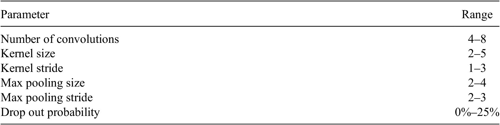
Table 2. Long description
The table consists of two columns: Parameter and Range.
* Number of convolutions: 4 to 8.
* Kernel size: 2 to 5.
* Kernel stride: 1 to 3.
* Max pooling size: 2 to 4.
* Max pooling stride: 2 to 3.
* Drop out probability: 0 percent to 25 percent.
Some of the most important training hyper-parameters are reported in Table 3. Figure 13 shows the loss convergence for the two training steps. Figure 13(a) shows a smooth convergence behavior for the low-fidelity training step. The case RANS + LES is shown in Figure 13(b); it exhibits more noise, but still demonstrates steady convergence. The difference in magnitude of the two losses is simply due to the different definition of the loss function in the two steps (see description of Eq. (4.1)).
Training hyper-parameters

Table 3. Long description
The table consists of two columns titled Hyper-parameter and Value.
* Batch size: 8.
* Validation set: 15%.
* Optimizer: Adam W (Loshchilov and Hutter, Reference Loshchilov and Hutter2019).
* Learning rate (eta): 5 times 10 super -4.
* Learning rate policy: Reduce on Plateau (Paszke et al., 2019).
* delta (of Eq. 4.1): 1.5.
Loss convergence for the two training steps. (a) step 1, RANS; (b) step 2, RANS+LES.

Figure 13. Long description
A two-panel line graph showing loss convergence. Both panels share a horizontal x-axis labeled Epoch ranging from 0 to 3000 and a vertical y-axis labeled Loss on a logarithmic scale from 10 super minus 3 to 10 super 0.
Panel a, labeled Training Step 1, R A N S. The graph shows two overlapping lines. The black line represents the Training set and the blue line represents the Validation set. Both lines show a steep asymptotic decrease from a loss of 10 super minus 1 at epoch 0, leveling off to a stable value just below 10 super minus 3 by epoch 2000. The curves are smooth with very minor oscillations.
Panel b, labeled Training Step 2, R A N S plus L E S. This graph also features a black line for the Training set and a blue line for the Validation set. Both lines show a rapid initial drop from 10 super 0 to approximately 10 super minus 2 within the first 200 epochs. Unlike panel a, these lines exhibit significant high-frequency noise and vertical spikes, particularly in the training set. The loss gradually stabilizes around 3 times 10 super minus 3 by epoch 3000, with the validation set showing slightly less volatility than the training set.
5.2.1. Encoding
Figure 14 shows the latent space obtained by encoding the multi-fidelity database. The black dots correspond to the low-fidelity data, while the red dots represent the high-fidelity data. A first observation is that for the RANS cases
$ {V}_1 $
 -
$ {V}_2 $
 -
$ {V}_3 $
 (the first latent subspace) is active, while
$ {V}_4 $
 -
$ {V}_5 $
 is not (all zero). In contrast, for the LES encoding, all latent variables are active. In
$ {V}_1 $
 -
$ {V}_2 $
 -
$ {V}_3 $
 , the red dots overlap with the black ones, indicating that this latent subspace is shared between the low- and high-fidelity datasets. To be precise,
$ {V}_4 $
 -
$ {V}_5 $
 are not exactly zero for RANS samples, because the conditioning is enforced through a soft penalty rather than a hard constraint. In our experiments, their magnitude is nearly zero for RANS cases, on the order of
$ \mathcal{O}\left({10}^{-5}\right) $
 , while for LES cases it is typically on the order of
$ \mathcal{O}\left({10}^{-1}\right) $
 . This behavior can be interpreted as
$ {V}_1 $
 -
$ {V}_2 $
 -
$ {V}_3 $
 being responsible for predicting the nozzle jet flow phenomenon in low fidelity, while
$ {V}_4 $
 -
$ {V}_5 $
 represent the correction term from low to high fidelity. In the present application, low- and high-fidelity data are two different representations of turbulence. RANS simulations are qualitatively correct and capture the physical phenomenon. Meanwhile, LES also capture the phenomenon quantitatively, as depicted in Figure 1 for the potential core region. For this reason, one can interpret the process as first learning a baseline (AE1) using RANS data, and then correcting (AE2) using LES data. It is expected that the structural, qualitative similarities between RANS and LES in this case enable a relatively small “latent space of corrections” (AE2 vs. AE1). If the differences between RANS and LES are more substantive, it is expected that the size of the latent correction would be considerably higher.
Latent space projections of the multi-fidelity database embeddings. Black dots correspond to the RANS latent representations; red dots to the LES latent representations.

Figure 14. Long description
The diagram consists of three main sections arranged horizontally.
1. On the far left, text reads R A N S in black and L E S in red, followed by the word database. An arrow points right toward the next section.
2. In the center is a gray trapezoidal block oriented vertically, labeled M B A encoder. An arrow points from this block to the right.
3. On the right is a triangular matrix of ten scatter plots representing latent space projections. The vertical Y axes are labeled V sub 2, V sub 3, V sub 4, and V sub 5 from top to bottom. The horizontal X axes are labeled V sub 1, V sub 2, V sub 3, and V sub 4 from left to right.
* The top row contains one plot (V sub 2 vs V sub 1) showing a dense cluster of black dots and scattered red dots near the origin.
* The second row contains two plots (V sub 3 vs V sub 1 and V sub 3 vs V sub 2) showing mixed black and red clusters.
* The third row contains three plots (V sub 4 vs V sub 1, V sub 2, and V sub 3). In these, black dots are strictly concentrated along the zero line of the Y axis, while red dots are scattered in the upper region.
* The bottom row contains four plots (V sub 5 vs V sub 1, V sub 2, V sub 3, and V sub 4). Similar to the third row, black dots remain at the zero baseline while red dots show a positive correlation trend, particularly in the V sub 5 vs V sub 4 plot at the bottom right.
Additionally, Figure 15 shows the projections of the latent space colored by the database design parameters. Only three projections are shown for the sake of clarity. The design parameters vary smoothly along the latent space, indicating that the AE learned these parameters automatically (they were not provided during training). By navigating the latent space, it is possible to generate predictions as function of the database parameters. A closer look reveals that
$ {V}_1 $
 varies with
$ {f}_A^{\ast } $
 ;
$ {V}_2 $
 with
$ {n}_{out} $
 , and
$ {V}_3 $
 with
$ {AR}_{out} $
 . Previous works in literature already found design parameters varying smoothly within the latent space of an AE for parametric datasets (Saetta et al., Reference Saetta, Tognaccini and Iaccarino2022; Fukami and Taira, Reference Fukami and Taira2023). Smoothness is not guaranteed in general but is promoted by the choice of continuous design variables and by inspecting that the resulting flow fields remain similar, so that the dataset maps a single regime of operations. It is very likely that in the presence of categorical design variables and extremely wide operating conditions, the resulting latent manifold would not be smooth.
Latent space projections colored by database design parameters. Blue: low parameter values; red: high parameter values.

Figure 15. Long description
A three-panel scatter plot series.
Panel (a) plots V 2 on the y-axis against V 1 on the x-axis. A color bar on the right for f sub A super asterisk ranges from 0.6 (blue) to 1.4 (red). Data points are clustered near the origin, with red points concentrated in the upper-left quadrant and blue points scattered toward the right.
Panel (b) plots V 3 on the y-axis against V 1 on the x-axis. The color bar for A R sub out ranges from 2 (blue) to 10 (red). The data shows a vertical gradient where red points are at the bottom (negative V 3) and blue points are at the top (positive V 3).
Panel (c) plots V 3 on the y-axis against V 2 on the x-axis. The color bar for n sub out ranges from 10 (blue) to 50 (red). The points form a curved, C-shaped distribution. Red and yellow points are concentrated in the center-right of the cluster, while blue points are distributed on the outer edges of the curve.
5.2.2. Decoding
Figure 16 illustrates the decoding procedure of the generative model:
-
1. A new set of design parameters (not used in training) is selected ( $ {f}_A^{\ast } $
,
$ {AR}_{out} $
and
$ {n}_{out} $
). -
2. The latent vector corresponding to such parameters is computed. Different strategies can be employed, such as fully connected neural networks or interpolations; in the present article, we opted for Radial Basis Functions (RBF). Specifically, we are interpolating a scalar field (one for each database parameter) over sparse points (the latent variables in a three-dimensional space) using RBF with a “Thin-Plate Spline” kernel. No smoothing parameter for the RBF is applied, that is, the interpolant passes through the known data points.
-
3. Feeding the latent vector to the decoder with $ {V}_4={V}_5=0 $
yields a low-fidelity (RANS) prediction. On the contrary, setting
$ {V}_4\ne 0 $
and
$ {V}_5\ne 0 $
produces a high-fidelity (LES) prediction.





Pipeline of multi-fidelity predictions using the trained ensemble of MBA decoders. Where
$ \overline{U} $
 is the non-dimensional velocity defined as
$ \overline{U}=U/{U}_j $
 and
$ {\overline{U}}_{LF} $
 and
$ {\overline{U}}_{HF} $
 are, respectively, referred to low and high fidelity.

Figure 16. Long description
The left side shows a flowchart starting with a box containing parameters f sub A super asterisk equals 0.86, A R sub out equals 3.0, and n sub out equals 30.0. Two paths emerge: a black path leading to a vector V with elements V sub 1, V sub 2, V sub 3, 0, 0; and a red path leading to a vector V with elements V sub 1 through V sub 5. Both paths enter a trapezoidal block labeled M B A decoder, which produces two output arrows.
The right side contains two vertically stacked line graphs with x-axes labeled x forward slash D sub e q ranging from -5 to 20.
Top graph: The y-axis is the absolute difference between U bar sub L F and U bar sub H F, ranging from 0.0 to 0.1. It compares C F D (black line) and A E (red line). Both lines show a peak near x forward slash D sub e q equals 5, with the C F D peak slightly higher at approximately 0.12 and the A E peak at 0.1.
Bottom graph: The y-axis is U bar, ranging from 0.5 to 1.0. It displays four curves: R A N S (dashed black), L E S (dashed red), A E minus L F (solid black), and A E minus H F (solid red). All curves show a steep increase to a plateau of 1.0 between x forward slash D sub e q equals 0 and 5, followed by a gradual non-linear decay toward 0.2 at x forward slash D sub e q equals 20.
The decoder is, therefore, a multi-fidelity model capable of predicting both RANS and LES fields. From an engineering perspective, only high-fidelity predictions are of interest. However, low-fidelity data are also important during training to cover regions where high-fidelity data are scarce (see Appendix C). In addition, as will be shown in Section 5.3, they improve the prediction accuracy of the high-fidelity fields.
The capability of the AE to capture the differences between low- and high-fidelity representations of the phenomenon is highlighted in Figure 16. For simplicity, only the streamwise velocity component along the
$ x $
 central axis is shown (bottom right). The differences between AE and the corresponding CFD results (both low and high fidelity) are barely visible, with errors below
$ 2\% $
 . The AE correctly captures the lack of accuracy of the low-fidelity representation in the potential core. The upper right plot shows the low-fidelity error (black for CFD, red for AE). The results are in agreement, indicating that the low-fidelity error reaches up to 10% in the potential core.
Global metrics (length of potential core
$ {L}_{pc} $
 and half-jet spreading at
$ x/{D}_{eq}=2 $
 for the entire LES dataset) are reported in Figure 17. The scatter plots lie along the red line
$ x=y $
 with negligible spreading. It indicates that the predicted fields preserve the accuracy of the global metrics which can be employed in an optimization objective function (see Appendix D).
Scatter plots of the predicted against the LES global metrics. (a) length of potential core
$ {L}_{pc} $
 ; (b) jet spreading
$ {y}_{1/2} $
 ; (c) jet spreading
$ {z}_{1/2} $
 at
$ x/{D}_{eq}=2 $
 .

Figure 17. Long description
A multi-panel figure containing three scatter plots. Each plot features a red diagonal line representing the identity function x equals y, with black circular data points distributed along or near this line.
Panel a, labeled L sub p c, shows L E S on the x-axis ranging from 1.0 to 4.0 and A E - H F on the y-axis ranging from 1.0 to 4.0. The data points follow a linear trend with some slight dispersion around the x equals y line, particularly between the values of 2 and 4.
Panel b, labeled y sub 1/2, shows L E S on the x-axis and A E - H F on the y-axis, both ranging from approximately 0.15 to 0.35. The data points are tightly clustered along the red x equals y line, indicating a very high correlation.
Panel c, labeled z sub 1/2, shows L E S on the x-axis and A E - H F on the y-axis, both ranging from approximately 0.4 to 1.1. Similar to panel b, the black data points are positioned almost exactly on the red diagonal line, showing a near-perfect linear relationship between the predicted and measured metrics.
5.3. High-fidelity predictions comparison with CFD simulations
The assessment of AE accuracy is performed on a case that was not used during training or validation. The selected design parameters are:
$ {f}_A^{\ast }=1.0 $
 ;
$ {AR}_{out}=10.0 $
 ;
$ {n}_{out}=30.0 $
 . The AE predicts the velocity field (and its standard deviation) as shown in Figure 18(a) that shows the streamwise velocity predicted over the entire field. This represents the mean velocity obtained from the uncertainty quantification analysis. Figure 18(b) shows the corresponding standard deviation, highlighting that the regions with higher uncertainties of the AE are along the jet short-side boundaries.
High-fidelity prediction of the MBA ensemble for
$ {f}_A^{\ast }=1.0 $
 ;
$ {AR}_{out}=10.0 $
 ;
$ {n}_{out}=30.0 $
 .

Figure 18. Long description
The figure consists of two panels, a and b, each showing a fluid flow simulation through a nozzle and into an open domain. A three-dimensional coordinate system is shown below each panel with y pointing up, x pointing right, and z pointing forward.
Panel a, labeled U all over U sub j, visualizes the mean velocity field. The flow enters from a transparent nozzle on the left, showing a transition from light blue to yellow. As it exits the nozzle, a solid red core indicates high velocity. Two vertical cross-sectional planes are positioned shortly after the nozzle exit, showing the internal velocity distribution. Further downstream, the flow expands and the velocity gradually decreases, transitioning from red to orange, yellow, and finally light blue at the far right.
Panel b, labeled Standard deviation, visualizes the uncertainty or variance in the prediction. The nozzle and the majority of the downstream flow are dark blue, indicating low standard deviation. However, the two vertical cross-sectional planes near the nozzle exit show concentrated pockets of green, yellow, and red, particularly at the shear layers or edges of the jet, indicating higher prediction uncertainty in those specific regions.
For a clear and quantitative analysis of AE performance, the results in the
$ x $
 -
$ z $
 plane are considered for the comparison with CFD data. Despite the training database being constructed using LES time averaged over
$ \overline{t_{sim}}=100 $
 , a comparison of AE predictions against LES averaged over
$ \overline{t_{sim}}=2000 $
 is also provided for this test case (not used in training). This comparison highlights an interesting feature of the proposed multi-fidelity method.
Figure 19 shows the mean (a) and standard deviation (b) of the prediction of the MBA ensemble. The mean appears smooth and symmetric, while the standard deviation highlights a small uncertain region around
$ x/{D}_{eq}=2.0 $
 , near the end of the potential core. Figure 20 shows the velocity field resulting from the LES averaged over
$ \overline{t_{sim}}=100 $
 (Figure 20(a)), and
$ \overline{t_{sim}}=2000 $
 (Figure 20(b)). The former exhibits a noisy and non-symmetric behavior, while the latter is more smooth. This difference is further illustrated in Figure 21, which shows the velocity profiles at different values of
$ x/{D}_{eq} $
 .
High-fidelity prediction of the MBA ensemble: mean prediction (a) and its standard deviation (b).
$ {f}_A^{\ast }=1.0 $
 ;
$ {AR}_{out}=10.0 $
 ;
$ {n}_{out}=30.0 $
 . Streamwise velocity contour maps on the
$ x $
 -
$ z $
 plane.

Figure 19. Long description
A two-panel visualization of fluid dynamics data. Both panels share a vertical axis labeled z all over D sub eq ranging from minus 5 to 5 and a horizontal axis ranging from 0 to 20.
Panel a, labeled A E prediction, displays the mean streamwise velocity. A vertical color bar on the right is labeled U all over U sub j with a scale from 0.000 in dark blue to 1.000 in dark red. The contour map shows a high-velocity core in dark red concentrated near the origin between x equals 0 and 5. As the flow moves right toward x equals 20, the velocity gradually decreases and the plume widens, transitioning through yellow, green, and light blue.
Panel b, labeled A E std, displays the standard deviation. The vertical color bar on the right is labeled S t d with a scale from 0.005 in dark blue to 0.125 in dark red. The map is predominantly dark blue, indicating low variance. Small regions of higher variance in light blue and green are visible near the nozzle exit at the origin and along the shear layers of the expanding plume.
Reference ground truth (GT): LES using
$ \overline{t_{sim}}=100 $
 (a) and using
$ \overline{t_{sim}}=2000 $
 (b) for the time averages.
$ {f}_A^{\ast }=1.0 $
 ;
$ {AR}_{out}=10.0 $
 ;
$ {n}_{out}=30.0 $
 . Velocity contour maps on the
$ x $
 -
$ z $
 plane.

Figure 20. Long description
A two-panel horizontal layout showing velocity contours.
Panel a, labeled G T with t sub sim bar equals 100, is on the left. The vertical y-axis is labeled z all over D sub e q, ranging from minus 5 to 5. The horizontal x-axis ranges from minus 5 to 20. A color bar on the right indicates U all over U sub j values from 0.000 in dark blue to 1.000 in dark red. The contour shows a high-velocity core (dark red) starting near x equals 0, which gradually tapers and dissipates into lower velocity regions (cyan and blue) as it moves right toward x equals 20. The edges of the flow appear slightly jagged or turbulent.
Panel b, labeled G T with t sub sim bar equals 2000, is on the right. It uses the same axes and color scale as Panel a. The central high-velocity core (dark red) is smoother and more symmetric compared to Panel a. The transition from the high-velocity red core to the low-velocity blue periphery is more uniform, reflecting the longer time average.
Comparison of LES using
$ \overline{t_{sim}}=100 $
 and
$ \overline{t_{sim}}=2000 $
 for the time averages.
$ {f}_A^{\ast }=1.0 $
 ;
$ {AR}_{out}=10.0 $
 ;
$ {n}_{out}=30.0 $
 . Velocity profiles at different stations downstream the nozzle outlet.

Figure 21. Long description
The x-axis represents normalized velocity U all over U sub j, ranging from 0.2 to 1.0. The y-axis represents a vertical spatial dimension from -1 to 1.
Top Legend:
- Black: x all over D sub e q = 1.8
- Red: x all over D sub e q = 5.0
- Blue: x all over D sub e q = 15.0
Bottom Legend:
- Solid line: t sub s i m bar = 2000
- Dashed line: t sub s i m bar = 100
Data Trends:
- At x all over D sub e q = 1.8 (rightmost, black), the profile is a wide top-hat shape centered at 0, with velocity near 1.0. The dashed line shows high-frequency fluctuations compared to the smooth solid line.
- At x all over D sub e q = 5.0 (middle, red), the profile has narrowed and the peak velocity has dropped to approximately 0.55. The dashed line shows significant jagged deviations from the solid curve.
- At x all over D sub e q = 15.0 (leftmost, blue), the profile is a narrow Gaussian-like curve with a peak velocity near 0.25. The dashed line continues to show more variance than the solid line.
Figure 22 shows the absolute percentage error maps between the MBA ensemble predictions and the two LES (not statistically converged (a) and converged (b)). Remarkably, although the MBA ensemble was trained using non-converged data, its prediction in Figure 19(a) is closer to the converged solution of Figure 20(b), as highlighted by the error maps of Figure 22. This behavior arises from the presence of RANS data and from the conditioning term we employ. In particular, during the first training step, AE1 is trained on RANS data, which are smooth and symmetric. As a result, the convolutional layers learn smooth feature maps and the symmetries of the flow. In addition, the RANS fields are qualitatively accurate enough to describe the underlying physics of the phenomenon. In the second step, AE2 is trained on both RANS and LES data, starting from the previously learned weights. Through the conditioning term, we guide the optimizer toward a solution that effectively corrects the RANS fields using LES data, also accounting for the symmetries still not completely captured by the not statistically converged LES simulations. Figure 23 presents a more detailed comparison between the MBA ensemble predictions and the LES averaged over
$ \overline{t_{sim}}=2000 $
 . The differences are within
$ 2\% $
 . To complete the analysis, Figure 24 shows the velocity field on the
$ y $
 -
$ z $
 plane at
$ x/{D}_{eq}=1 $
 . Figures 24(a) and 24(b) show the LES results and the MBA predictions, respectively. Figures 24(c) and 24(d) present the local error (with respect to the ground truth) and the standard deviation of the prediction, respectively. The largest errors are confined to the corners of the jet. The standard deviation clearly mirrors the error distribution, providing an effective way to identify regions of largest uncertainty when the ground truth is not available (see also Saetta et al. (Reference Saetta, Tognaccini and Iaccarino2024)). Table 4 reports the global parameters computed from the LES and predicted fields, demonstrating the accuracy of the AE in predicting the control parameters. A larger error is present in the computation of
$ {L}_{pc} $
 (as confirmed by the error peak in Figure 23), but it remains negligible compared to the overall phenomenon (see Figure 17). The low-fidelity data guide the symmetry and the smoothness of the phenomenon, while the additional latent variables provide the high-fidelity correction. Indeed, the analysis using only a single-fidelity database with 20 LES for training, reported in Appendix C, shows that in the absence of low-fidelity data, the predictions are noisy and non-symmetric.
MBA prediction errors with LES using
$ \overline{t_{sim}}=100 $
 (a) and using
$ \overline{t_{sim}}=2000 $
 (b) for the time averages.
$ {f}_A^{\ast }=1.0 $
 ;
$ {AR}_{out}=10.0 $
 ;
$ {n}_{out}=30.0 $
 . Velocity contour maps on the
$ x $
 -
$ z $
 plane.

Figure 22. Long description
A two-panel figure showing velocity contour maps on the x-z plane. Both panels share a vertical y-axis labeled z all over D sub eq ranging from minus 5 to 5 and a horizontal x-axis ranging from minus 2 to 20. A color scale on the right of each panel indicates percentage error from 0.00 in dark blue to 10.00 in dark red.
Panel a, labeled percent Error minus G T with t sub sim bar equals 100, shows a plume-like shape starting at x equals 0. The interior of the plume is predominantly dark blue with significant patches of light blue, green, and yellow, indicating higher error levels between 3.75 and 6.25 percent, particularly in the region between x equals 5 and x equals 15.
Panel b, labeled percent Error minus G T with t sub sim bar equals 2000, shows the same plume shape. In this panel, the interior is almost entirely dark blue, indicating a much lower error rate, generally below 1.25 percent, across the entire domain. Only a small vertical band of light blue and green appears near x equals 2.
High-fidelity prediction of the MBA ensemble and reference CFD simulation (LES using
$ \overline{t_{sim}}=2000 $
 ) for
$ {f}_A^{\ast }=1.0 $
 ;
$ {AR}_{out}=10.0 $
 ;
$ {n}_{out}=30.0 $
 . (a) Velocity along the central nozzle axis; (b) velocity profiles at different stations downstream the nozzle outlet.

Figure 23. Long description
A multi-panel figure consisting of two main sections labeled a and b.
Panel a contains two stacked line graphs with a shared x-axis representing x all over D sub e q ranging from -5 to 20.
- The top graph plots Std in blue and percentage Error in red. The blue line remains relatively flat near 1.0, while the red line shows a sharp peak of approximately 4.0 near x all over D sub e q equals 3 before fluctuating at lower values.
- The bottom graph plots U all over U sub j. A black line for L E S and a red line for A E prediction are nearly identical, showing a steep rise to a peak of 1.0 at x equals 0, followed by an asymptotic decay toward 0.2.
Panel b is a single plot showing three vertical velocity profiles. The x-axis is U all over U sub j from 0.2 to 1.0, and the y-axis is unlabeled but represents radial position from -1.5 to 1.5.
- The rightmost profile at x all over D sub e q equals 1.8 is black, showing a wide top-hat shape with a flat peak near 1.0.
- The middle profile at x all over D sub e q equals 5.0 is red, showing a narrower, slightly rounded peak near 0.6.
- The leftmost profile at x all over D sub e q equals 15.0 is blue, showing a sharp, narrow peak near 0.25.
In all three profiles, solid lines represent L E S and dashed lines represent A E prediction, with shaded regions indicating the ensemble variance. The A E predictions closely follow the L E S data across all stations.
High-fidelity prediction of the MBA ensemble and reference CFD simulation (LES using
$ \overline{t_{sim}}=2000 $
 ) for
$ {f}_A^{\ast }=1.0 $
 ;
$ {AR}_{out}=10.0 $
 ;
$ {n}_{out}=30.0 $
 . Velocity contour map in the
$ y $
 -
$ z $
 plane at
$ x/{D}_{eq}=1 $
 .

Figure 24. Long description
A multi-panel visualization consisting of four subplots arranged in a two-by-two grid. All subplots share the same axes: the horizontal axis is z forward slash D sub eq ranging from minus 2 to 2, and the vertical axis is y forward slash D sub eq ranging from minus 0.5 to 0.5.
* Top-left panel (a) G T: Displays a rectangular velocity profile with a high-velocity red core (U forward slash U sub j approximately 1.0) surrounded by a thin gradient transitioning through yellow and green to a blue low-velocity background. A color bar on the right scales from 0.000 to 1.000.
* Top-right panel (b) M B A: Shows a nearly identical velocity profile to panel (a), representing the model prediction. The color bar scale is identical to panel (a).
* Bottom-left panel (c) percent error: Visualizes the difference between G T and M B A. The plot is mostly dark blue (near 0 percent error) with small localized peaks of light blue and yellow (up to 10 percent) concentrated at the four corners of the rectangular jet boundary. The color bar scales from 0.00 to 10.00 percent Err.
* Bottom-right panel (d) Standard Deviation: Shows the uncertainty of the ensemble. High uncertainty (red/yellow spots) is concentrated at the four corners of the jet, mirroring the error distribution in panel (c). The color bar scales from 0.004 to 0.076 Std.
Control parameters computed in the predicted and LES fields for
$ {f}_A^{\ast }=1.0 $
 ;
$ {AR}_{out}=10.0 $
 ;
$ {n}_{out}=30.0 $


Table 4. Long description
The table consists of four columns and three rows including the header.
Column headers from left to right are:
1. An empty cell for the model type.
2. L sub p c.
3. y sub 1/2.
4. z sub 1/2.
Row 1 (L E S):
- L sub p c is 1.06.
- y sub 1/2 is 0.13.
- z sub 1/2 is 1.11.
Row 2 (A E prediction):
- L sub p c is 1.31.
- y sub 1/2 is 0.13.
- z sub 1/2 is 1.09.
In this case, the multi-fidelity method (compared to the standard single-fidelity approach) reduces the computational cost in two ways: by requiring a limited number of costly high-fidelity data and by allowing LES performed with a limited number of time steps (an order of magnitude lower). Table 5, which reports the computational cost for the entire setup (database construction and model training), highlights the savings achieved with this method. The accuracy of the predictive methods trained on single- and multi-fidelity shows that the best overall performance is achieved by the multi-fidelity approach. With only a small increase in computational cost compared to the HF-
$ \overline{t_{sim}}=100 $
 case, the error in jet spreading is reduced by one order of magnitude for
$ {y}_{1/2} $
 and by two orders of magnitude for
$ {z}_{1/2} $
 . The error in the potential core length
$ {L}_{pc} $
 is higher, but the difference is negligible (moreover, Table A3 shows that adding one latent variable on the multi-fidelity case improves the prediction of
$ {L}_{pc} $
 ). The cost of constructing the HF-
$ \overline{t_{sim}}=2000 $
 database is prohibitive and is therefore not considered in this analysis. Indeed, this is exactly the reason why multi-fidelity methods are necessary for these types of applications.
Computational cost and overall accuracy on the global parameters

Table 5. Long description
The table consists of six columns: Model Type, Number of cases, Cost, M S E L sub p c, M S E y sub 1/2, and M S E z sub 1/2.
* L F: 92 cases; Cost approximately 11.2 k C P U h; M S E L sub p c is 8.16 times 10 super minus 1; M S E y sub 1/2 is 1.03 times 10 super minus 4; M S E z sub 1/2 is 5.73 times 10 super minus 3.
* H F with t sub sim bar equals 100: 20 cases; Cost approximately 906 k C P U h; M S E L sub p c is 3.76 times 10 super minus 2; M S E y sub 1/2 is 4.31 times 10 super minus 5; M S E z sub 1/2 is 1.01 times 10 super minus 3.
* Multi-fidelity: 112 cases; Cost approximately 917 k C P U h; M S E L sub p c is 9.64 times 10 super minus 2; M S E y sub 1/2 is 3.71 times 10 super minus 6; M S E z sub 1/2 is 5.20 times 10 super minus 5.
* H F with t sub sim bar equals 2000: 92 cases; Cost approximately 30.6 M C P U h; M S E values are not provided for this row.
6. Using the latent space for shape optimization
As previously discussed, the trained multi-fidelity MBA ensemble can be used within an optimization loop to accelerate the design of nozzle shapes. By sampling the latent space, it is possible to generate a large number of flow predictions in real time and compute the quantities of interest (
$ {L}_{pc} $
 ,
$ {y}_{1/2} $
 , and
$ {z}_{1/2} $
 ), thereby mapping the latent space by assigning these quantities to each combination of latent variables. Employing this methodology enables the navigation of the latent space to find the combination of latent variables that minimizes jet extension (lowest values of
$ {L}_{pc} $
 ) and maximizes jet spreading (
$ {y}_{1/2} $
 and
$ {z}_{1/2} $
 ), thereby enhancing jet mixing with the outer flow. The objective of this analysis is to illustrate the advantages of employing the multi-fidelity MBA ensemble as opposed to conducting a full nozzle optimization and should be seen as a proof-of-concept study. As illustrated in Figure 25, the latent space projections are mapped with the global parameters. This represents, in practice, the optimization landscape with the objective function
$ \min \left({L}_{pc}\right) $
 and parameters
$ {V}_i $
 ,
$ i=1,\dots, 5 $
 . It was obtained by performing 10000 flow predictions using the trained decoder, which would be unfeasible with CFD simulations. For clear visualization, an interpolation on a finer grid (5000
$ \times $
 5000 points) was performed using RBF with a thin-plate spline kernel. For brevity, the same analysis for the other parameters of interest is not reported but exhibits similar behavior.
Visualization of the global parameter
$ {L}_{pc} $
 along the latent space projections.

Figure 25. Long description
A four-panel visualization of three-dimensional surface plots. Each plot uses a color gradient where blue represents lower values and red represents higher values of L sub p c.
* Panel a, top-left. The x-axis is V sub 1 from 0.05 to 0.35, the y-axis is V sub 2 from -2 to 1, and the z-axis is L sub p c from 1.35 to 1.55. The surface shows a prominent central ridge that peaks near V sub 1 equals 0.15 and V sub 2 equals 0, sloping downward toward the edges.
* Panel b, top-right. The x-axis is V sub 2 from -2 to 1, the y-axis is V sub 3 from -2 to 2, and the z-axis is L sub p c from 1.35 to 1.50. The surface is more irregular with multiple peaks in the red-orange range and a deep blue trough in the foreground at low V sub 2 and V sub 3 values.
* Panel c, bottom-left. The x-axis is V sub 3 from -2 to 2, the y-axis is V sub 4 from 0.1 to 0.6, and the z-axis is L sub p c from 1.40 to 1.54. The surface features a high ridge running along the back of the plot at higher V sub 4 values, with a sharp decline toward the front-left corner.
* Panel d, bottom-right. The x-axis is V sub 4 from 0.1 to 0.6, the y-axis is V sub 5 from -0.5 to -0.1, and the z-axis is L sub p c from 1.42 to 1.52. This surface is the flattest of the four, showing a gentle valley in the center with higher values concentrated at the extreme corners of the V sub 4 and V sub 5 ranges.
Considering the values of the generated latent vectors, the best combination for minimizing
$ {L}_{pc} $
 corresponds to a nozzle with
$ {f}_A^{\ast }=0.500 $
 ,
$ {AR}_{out}=9.501 $
 , and
$ {n}_{out}=15.554 $
 . For this geometry,
$ {L}_{pc}=1.278 $
 m,
$ {y}_{1/2}=0.123 $
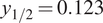 m, and
$ {z}_{1/2}=1.079 $
 m. However, all the parameters of interest need to be optimized. To find the best compromise for minimizing overall jet extension, we performed a simple analysis: first, the parameters were scaled between 0 and 1; then, a weighted sum,
$ 0.5\cdot {L}_{pc}+0.25\cdot \frac{1}{y_{1/2}}+0.25\cdot \frac{1}{z_{1/2}} $
 , was computed, and the minimum was identified. The weighting is introduced to ensure that the potential core length and the jet spreading contribute equally to the optimization. Note that this objective function considers only the components of the jet along the y- and z-directions and does not account for the full jet cross-section or overall spreading. The corresponding nozzle geometry resulting from the conceptual optimization is
$ {f}_A^{\ast }=0.977 $
 ,
$ {AR}_{out}=3.093 $
 , and
$ {n}_{out}=2.018 $
 , with global parameters
$ {L}_{pc}=2.887 $
 m,
$ {y}_{1/2}=0.214 $
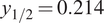 m, and
$ {z}_{1/2}=0.675 $
 m. The velocity predictions for the minimum
$ {L}_{pc} $
 nozzle and the best nozzle geometry are shown in Figure 26. To better illustrate the selection of the best compromise between potential core length and jet spreading, Figure 27 shows the Pareto front associated with the two objective functions. The black dots represent the 10000 realizations obtained by sampling the latent space, whereas the red star denotes the selected case identified through the optimization procedure. This result does not represent an optimized nozzle, as it corresponds to the best among the 10000 generated samples. To identify the best geometry, a formal optimization procedure would be required.
Velocity contour map corresponding to (a) the nozzle providing the minimum
$ {L}_{pc} $
 :
$ {f}_A^{\ast }=0.500 $
 ,
$ {AR}_{out}=9.501 $
 , and
$ {n}_{out}=15.554 $
 ; (b) the nozzle geometry providing the best compromise between potential core length and jet spreading:
$ {f}_A^{\ast }=0.977 $
 ,
$ {AR}_{out}=3.093 $
 , and
$ {n}_{out}=2.018 $
 .

Figure 26. Long description
The figure consists of two panels, labeled (a) and (b), each showing a three-dimensional velocity contour map of a nozzle and its resulting jet. Below each panel is a coordinate system with y pointing up, x pointing right, and z pointing forward.
* Panel (a) Minimum L sub p c: Shows a nozzle with a wide, flat inlet that tapers. The velocity is highest (red) at the inlet and decreases rapidly as the flow exits the nozzle. The jet plume is short and dissipates into lower velocity (blue) quickly along the x-axis.
* Panel (b) Best compromise: Shows a nozzle with a similar tapering geometry but a different aspect ratio. The high-velocity core (red and orange) extends significantly further downstream from the nozzle exit compared to panel (a), indicating a longer potential core and more sustained jet spreading.
In both panels, the flow passes through two rectangular vertical cross-sections that highlight the internal velocity distribution before the jet expands into the open domain.
Pareto front of the optimization procedure sampling 10000 latent vectors. Objective function minimization: potential core length
$ {L}_{pc} $
 and jet spreading
$ \frac{1}{y_{1/2}}+\frac{1}{z_{1/2}} $
 . Red star: best selected case.

Figure 27. Long description
The scatter plot is set on a grid with the horizontal x axis labeled L sub p c ranging from 1 to 5 and the vertical y axis labeled 1 all over y sub 1/2 plus 1 all over z sub 1/2 ranging from 5 to 9. The data consists of approximately 10000 black semi-transparent circular points that form a dense downward-sloping curve from the top-left to the bottom-right. At the left side of the graph where L sub p c is approximately 1.5, the y values are highest near 9. As L sub p c increases toward 5, the y values decrease asymptotically toward 5. A single red star is positioned slightly below the main dense cluster at approximately x equals 2.9 and y equals 6.2, representing the best selected case.
7. Conclusions
The present article proposes a set of multi-fidelity, multi-branch AEs for predicting high-fidelity flows with quantified uncertainties while limiting the computational effort required to construct the training database. Specifically, three ML methods (a multi-branch AE architecture, a multi-fidelity training algorithm for AEs, and an ensemble technique for quantifying the prediction uncertainties) have been combined to build a unified training pipeline.
The proposed method was applied to a problem of practical engineering interest: nozzle jet flow prediction. Specifically, the multi-fidelity model was constructed using a database composed of many RANS simulations (low fidelity) and only a few LES (high fidelity). The result is a multi-fidelity model capable of predicting both low- and high-fidelity data across the entire design space. High-fidelity predictions with quantified uncertainty were obtained in real time, with an average error of approximately 2%. The small number of high-fidelity samples enabled the construction of a correction term from low to high fidelity.
In contrast to standard single-fidelity training procedures, the present approach drastically reduces the computational cost associated with database construction (by more than 30 times in the present test). The computational savings from using the multi-fidelity algorithm are twofold: only a small fraction of LES are needed, and the LES time averages can be obtained by reducing the number of time steps required for the statistics computation by an order of magnitude.
Finally, we showed that by predicting a large number of flow fields (10000) using the decoder and computing the parameters of interest for each field, it is possible to visualize them as a function of the latent variables. In this way, we can identify the optimized nozzle geometry through latent space analysis with minimal computational effort. Performing the same analysis using CFD simulations would be computationally unfeasible.
Data availability statement
The data that support the findings are openly available in the “Multi-Fidelity Nozzle Jet Flows” repository on Hugging Face: https://huggingface.co/datasets/taarg/MultiFidelity_Nozzle_JetFlows.
Acknowledgements
We acknowledge ISCRA for awarding this project access to the LEONARDO supercomputer, owned by the EuroHPC Joint Undertaking, hosted by CINECA (Italy).
Author contribution
Conceptualization: E.S., M.M., R.T., G.I.; Data curation: E.S., M.M., R.T., G.I.; Methodology: E.S., M.M., R.T., G.I.
Funding statement
This work received no specific grant from any funding agency, commercial, or not-for-profit sectors.
Competing interests
The author(s) declare none.
Ethical standards
The research meets all ethical guidelines, including adherence to the legal requirements of the study country.
A. Sensitivity analysis of the latent space dimension
The size of the latent variable is a critical hyper-parameter in this problem. We choose to treat it as a control parameter, performing training with an increasing size and stopping when a further increase in latent dimensions does not lead to better loss reduction. The resulting minimum dimension effectively represents the dimensionality of the latent manifold.
The present database was generated using three precise independent design parameters for the geometry of the nozzle. Therefore, the expectation is that the minimum dimensionality of the latent space is 3 (it could be lower if the design parameters are not independent). In more complex situations and if the resulting flow fields span different regimes, it is possible that the latent manifold requires a larger number of dimensions. In general, keeping the latent space small can facilitate interpretation.
We performed a sensitivity analysis on the latent space dimension for the first training step; the results are reported in Table A1. The analysis included the
$ {R}^2 $
 regression score, the explained variance, and the Structural Similarity Index Measure (SSIM). To define a criterion for selecting the minimum number of required latent variables, we rely on other works in literature: for POD, this corresponds to retaining the smallest number of modes that capture at least 99% of the explained variance, which is a standard criterion in the literature (Brindise and Vlachos, Reference Brindise and Vlachos2017; Tang et al., Reference Tang, Fang, Zheng and Tao2025). Similarly, in our case, sufficiency was defined as the smallest latent dimension for which the reconstruction metric considered here (i.e.,
$ {R}^2 $
 ) reached 0.99 and showed no substantial further improvement with additional latent variables. While this convergence criterion with increasing number of modes is mathematically guaranteed for POD in terms of reconstruction error reduction, it is not generally guaranteed for deep learning algorithms. However, similar analyses are commonly adopted in autoencoder-based reduced-order models and should be interpreted solely as a convergence study with respect to the latent space dimension (Ngoc and Hwang, Reference Ngoc and Hwang2020; Baig et al., Reference Baig, Ma, Xu and You2023).
As shown in Table A1, with only two latent variables, we already reach
$ {R}^2=0.994 $
 . This is because the
$ {n}_{out} $
 design parameter has a minimal influence on the solution field. However, neglecting this parameter prevents us from distinguishing between rectangular and elliptical outlet sections. For this reason, we introduced a third latent variable to also capture the small effects of
$ {n}_{out} $
 (see Figure 15). Thus, the third latent variable can be seen as a service variable which is not introduced to improve the aggregate error, but to preserve the full parametric description of the problem. Adding more than three latent variables would not significantly improve the model performance.
AE1 training

Table A1. Long description
The table consists of six columns and six rows including the header.
Column headers from left to right are: l.v. (latent variables), Avg. training time, Avg. inference time, R super 2, Exp. Var., and S S I M.
Data rows are as follows:
* Row 1: l.v. 1, 6.317 min, 0.0368 sec, 0.984, 0.984, 0.993.
* Row 2: l.v. 2, 6.264 min, 0.0358 sec, 0.994, 0.994, 0.996.
* Row 3: l.v. 3, 6.257 min, 0.0350 sec, 0.995, 0.995, 0.997.
* Row 4: l.v. 4, 6.260 min, 0.0346 sec, 0.996, 0.996, 0.997.
* Row 5: l.v. 5, 6.282 min, 0.0336 sec, 0.996, 0.996, 0.997.
Performance metrics show a trend where increasing latent variables from 1 to 5 generally improves R super 2 and S S I M values while slightly decreasing inference time.
For the analysis of the latent space dimension of the second training step, the number of latent variables for AE1 (i.e., using only LF data) is fixed at 3.
We performed three different trainings of the multi-fidelity MBA ensemble, considering 1, 2, and 3 additional latent variables to map the correction term from LF to HF. A first analysis of the computational cost and prediction accuracy metrics is presented in Table A2. The results indicate that one additional latent variable is sufficient to map the correction between RANS and LES: R2 and explained variance are both >99%.
AE2 training

Table A2. Long description
The table consists of six columns and four rows.
Columns from left to right are:
1. l.v. (latent variables)
2. Avg. training time
3. Avg. inference time
4. R super 2
5. Exp. Var. (Explained Variance)
6. S S I M (Structural Similarity Index Measure)
Data rows:
- Row 1: l.v. plus 1; Avg. training time 19.0240 min; Avg. inference time 0.0352 sec; R super 2 0.993; Exp. Var. 0.993; S S I M 0.962.
- Row 2: l.v. plus 2; Avg. training time 16.805 min; Avg. inference time 0.0345 sec; R super 2 0.995; Exp. Var. 0.995; S S I M 0.967.
- Row 3: l.v. plus 3; Avg. training time 18.710 min; Avg. inference time 0.0348 sec; R super 2 0.997; Exp. Var. 0.997; S S I M 0.971.
Note: Metrics are for a multi-fidelity R A N S minus L E S model using an M B A ensemble with 50 elements and 3 latent variables for A E super 1. Hardware used was N V I D I A R T X 6000 Ada.
To better assess the predictive performance, an analysis of the physical variables and quantities of interest (
$ {L}_{pc} $
 ,
$ {y}_{1/2} $
 , and
$ {z}_{1/2} $
 ) is required. The prediction of axial velocity along the central nozzle axis is shown in Figure A1. The predictions obtained by adding 1 latent variable are already accurate. However, the upper plots of Figure A1, which show the difference between HF and LF data (
$ \mid {\overline{U}}_{LF}-{\overline{U}}_{HF}\mid $
 , which is interpretable as the correction term), indicate a convergent behavior toward the LES data as the latent space dimension increases. The result is confirmed by the trend of the global parameters monitored in Table A3. The results obtained by adding two latent variables are already satisfactory, and this is the one considered in the article to balance the accuracy and the compression rate.
Streamwise velocity on the nozzle central axis. Multi-fidelity predictions using 1, 2, and 3 additional latent dimensions for the second (HF) training step.
$ {f}_A^{\ast }=0.86 $
 ,
$ {AR}_{out}=3.0 $
 ,
$ {n}_{oout}=30.0 $
 .

Figure A1. Long description
A multi-panel figure consisting of three columns labeled a, b, and c.
Column a, titled plus 1 latent variable, contains two line graphs. The top graph shows the absolute difference between U sub L F and U sub H F on the y-axis ranging from 0.0 to 0.1, against x all over D sub e q on the x-axis from minus 5 to 20. It compares C F D in black and A E in red, showing a peak error near x equals 5. The bottom graph shows mean velocity U bar from 0.0 to 1.0. It plots R A N S as a dashed black line, L E S as a dashed red line, A E minus L F as a solid black line, and A E minus H F as a solid red line. The curves rise sharply to 1.0 at x equals 0 and decay gradually after x equals 5.
Column b, titled plus 2 latent variables, follows the same layout. The top error graph shows the red A E line more closely following the black C F D line compared to column a. The bottom velocity graph shows the solid red A E minus H F line shifting closer to the solid black A E minus L F line in the decay region between x equals 5 and 15.
Column c, titled plus 3 latent variables, shows the highest convergence. In the top error graph, the A E and C F D lines are nearly overlapping. In the bottom velocity graph, the A E minus H F and A E minus L F curves are almost identical, indicating that increasing latent dimensions improves multi-fidelity prediction accuracy.
Control parameters computed in the predicted and LES fields using 1, 2, and 3 additional latent dimensions

Table A3. Long description
The table consists of four columns and five rows including the header.
* Header Row: The first column is blank. The second column is L sub p c. The third column is y sub 1/2. The fourth column is z sub 1/2.
* Row 2 (L E S): L sub p c is 1.06, y sub 1/2 is 0.13, and z sub 1/2 is 1.11.
* Row 3 (A E - plus 1 l.v.): L sub p c is 1.42, y sub 1/2 is 0.13 (bold), and z sub 1/2 is 1.07.
* Row 4 (A E - plus 2 l.v.): L sub p c is 1.31, y sub 1/2 is 0.13 (bold), and z sub 1/2 is 1.09 (bold).
* Row 5 (A E - plus 3 l.v.): L sub p c is 1.13 (bold), y sub 1/2 is 0.13 (bold), and z sub 1/2 is 1.09 (bold).
A footnote indicates that f sub A super asterisk equals 1.0, A R sub out equals 10.0, and n sub out equals 30.0. Bold values represent the best results relative to the L E S baseline.
Regarding the training and inference costs when varying the number of latent variables, these are reported in Tables A1 and A2. It is clear that they are not significantly affected by the size of the latent space and remain negligible compared to the CFD cost (Table 5).
B. Sensitivity analysis on the MBA ensemble dimension
To quantify the model-form uncertainties in the predictions, we adopted an ensemble technique involving an ensemble of 50 MBAs. Here, we illustrate a sensitivity analysis of the ensemble dimension, as well as an analysis of the individual MBA realizations within the ensemble.
Figure B1 shows the standard deviation (i.e., uncertainty) of the predicted velocity along the central nozzle axis for an LES prediction with
$ {f}_A^{\ast }=1.0 $
 ,
$ {AR}_{out}=10.0 $
 , and
$ {n}_{out}=30.0 $
 , for different ensemble dimensions. Using only 10 items is insufficient to compute meaningful statistics on the model uncertainty as this leads to an underestimation of variability. By contrast, using 50, 100, and 200 items exhibits a convergent behavior. An ensemble of 50 MBAs is already sufficient to capture the uncertainty induced by model variability.
Standard deviation of the prediction of velocity along the central nozzle axis LES for
$ {f}_A^{\ast }=1.0 $
 ;
$ {AR}_{out}=10.0 $
 ;
$ {n}_{out}=30.0 $
 and different dimensions of the MBA ensembles. Dotted magenta: 10; dashed blue: 50; dot-dash red: 100; continuous black: 200.

Figure B1. Long description
The x-axis is labeled x forward slash D sub e q and ranges from negative 5 to 20. The y-axis is labeled S t d and ranges from 0.00 to 0.04. Four curves represent different M B A ensemble sizes.
* Dotted magenta line (10): Remains nearly flat and close to the zero baseline across the entire x-range with minor oscillations.
* Dashed blue line (50): Shows the highest peaks, with a sharp spike at x equals negative 2, a major peak reaching 0.026 at x equals 5, and a secondary peak at x equals 8.
* Dot-dash red line (100): Follows the same profile as the blue line but with lower intensity, peaking at approximately 0.021 at x equals 5.
* Continuous black line (200): Follows the same profile as the red and blue lines but with the lowest intensity of the three, peaking at approximately 0.018 at x equals 5.
All three higher-order curves (50, 100, 200) converge toward lower values between x equals 0 and 3, and again between x equals 12 and 18, before showing a slight upward trend at the far right of the graph.
Figure B2 shows the predictions of each ensemble member for the same case (LES with
$ {f}_A^{\ast }=1.0 $
 ,
$ {AR}_{out}=10.0 $
 , and
$ {n}_{out}=30.0 $
 ). The mean and median predictions are also reported and overlap, proving that the final predictions we reported are robust to the presence of outliers. Figure B2 also shows that the ensemble members are representative of the variability in the model. The region of the jet core decay exhibits the highest variability, due to the notorious tendency of RANS predictions to overestimate turbulent mixing in the jet shear layers, thus increasing the length of the jet core (see Figure 1).
Velocity along the central nozzle axis. Mean prediction (blue), median prediction (red), and item prediction (gray) for LES of
$ {f}_A^{\ast }=1.0 $
 ;
$ {AR}_{out}=10.0 $
 ;
$ {n}_{out}=30.0 $
 . (a) whole prediction; (b) zoom around the ending of the potential core jet.

Figure B2. Long description
Two panels labeled a and b. Both graphs share the same axes: the x-axis is x forward slash D sub e q and the y-axis is U forward slash U sub j.
Panel a: The x-axis ranges from negative 5 to 20. The y-axis ranges from 0.2 to 1.0. Multiple gray lines represent item predictions. A thick red line represents the median prediction and a blue line represents the mean prediction. The data shows a sharp increase from x equals negative 5 to 0, reaching a plateau at 1.0. From x equals 5 to 20, the velocity follows a non-linear decay curve down to approximately 0.2.
Panel b: A zoomed view of the potential core jet ending. The x-axis ranges from 2.0 to 5.0 and the y-axis ranges from 0.850 to 1.000. The gray item prediction lines show significant variance, with some staying near 1.0 until x equals 4.5. The red median and blue mean lines are closely aligned, showing a steady decline starting around x equals 3.0, dropping from 1.0 to approximately 0.86 at x equals 5.0.
C. Multi-fidelity vs. LES single-fidelity
In this Appendix, results are reported using a standard single-fidelity approach with the available LES dataset, highlighting the difficulties of training an AE with a very limited high-fidelity database. The AE model employed here is an ensemble of MBAs, as described in Section 4. Figure C1 shows the latent space projections colored by database design parameters. For
$ {AR}_{out} $
 , the latent variables are smooth and well organized, whereas the other two parameters were not effectively captured by the training. This can be explained by Table C1, which reports the correlation between the design parameters and the
$ {L}^2 $
 norm of the discretized velocity field (a measure of energy content) using the Pearson correlation index
$ r $
 (Freedman et al., Reference Freedman, Pisani and Purves2007). Values of
$ \mid r\mid \to 1 $
 indicate high correlation, while
$ \mid r\mid \to 0 $
 indicates low correlation. It shows that the most important parameter is
$ {AR}_{out} $
 , followed by a very low influence of
$ {f}_A^{\ast } $
 and
$ {n}_{out} $
 . One way to capture parameters with lower influence on the flow fields is to include more data representing this variability. However, this would require additional LES samples, further increasing the computational cost.
Latent space projections colored by database design parameters. Blue: low parameter values; red: high parameter values. Single-fidelity method using the LES database.

Figure C1. Long description
The image consists of three panels labeled a, b, and c. Each panel displays a matrix of three scatter plots showing the relationship between latent variables V 1, V 2, and V 3.
Panel a is titled f super asterisk sub A coloring. It contains three plots: V 2 versus V 1 at the top left, V 3 versus V 1 at the bottom left, and V 3 versus V 2 at the bottom right. Data points are colored according to a scale from 0.6 blue to 1.4 red. The distribution shows a mix of colors with no dominant linear trend.
Panel b is titled A R sub out coloring. It uses the same three-plot matrix structure. The color bar ranges from 1 blue to 10 red. In the V 3 versus V 2 plot, there is a slight concentration of higher red values toward the right side of the cluster.
Panel c is titled n sub out coloring. It follows the same matrix structure. The color bar ranges from 0 blue to 50 red. The data points appear predominantly blue and green, indicating lower parameter values across the latent space projections.
All plots share common axes: V 1 and V 2 on the horizontal axes ranging from -1 to 1, and V 2 and V 3 on the vertical axes ranging from -2 to 2. The L E S database refers to Large Eddy Simulation.
Pearson correlation index r describing the correlation between the design parameters and the L2 norm of the velocity field (a measure of the energy content)

Table C1. Long description
The table consists of one header row and one data row.
Header Row:
- The first column is empty.
- The second column is labeled f sub A super asterisk.
- The third column is labeled A R sub out.
- The fourth column is labeled n sub out.
Data Row:
- The first column contains the absolute value of r.
- The second column (under f sub A super asterisk) has a value of 0.173.
- The third column (under A R sub out) has a value of 0.980.
- The fourth column (under n sub out) has a value of 0.020.
The velocity contour map and its standard deviation on the x-z plane are reported in Figure C2. The single-fidelity prediction is noisy and non-symmetric. Moreover, Figure C2(d) shows large errors inside the nozzle, caused by the AE’s inability to identify the
$ {f}_A^{\ast } $
 parameter. The UQ analysis (standard deviation in Figure C2(b)) highlights the difficulty of predicting this region, with high uncertainty inside the nozzle. The prediction of the global parameters reported in Table C2 shows good accuracy, even though only the
$ {AR}_{out} $
 design parameter is captured indicative of the fact that the leading design parameter is sufficient for the assessment of the global parameters.
Prediction of the MBA ensemble (single-fidelity model) and reference ground truth (GT) for
$ {f}_A^{\ast }=1.0 $
 ;
$ {AR}_{out}=10.0 $
 ;
$ {n}_{out}=30.0 $
 . Velocity contour maps on the x-z plane.

Figure C2. Long description
A four-panel grid of velocity contour maps. All panels share a horizontal x-axis from -5 to 20 and a vertical z all over D sub eq axis from -5 to 5.
* Top-left panel (a) A E prediction: Shows a horizontal plume expanding from left to right. A high-velocity core in dark red (1.000) is centered near x equals 0, tapering through yellow and green to a blue low-velocity region (0.000) at x equals 20. The color bar is labeled U all over U sub j.
* Bottom-left panel (c) G T minus L E S: Displays a nearly identical velocity distribution to panel (a), serving as the ground truth reference. The color bar is also labeled U all over U sub j.
* Top-right panel (b) A E standard deviation: Shows the uncertainty of the prediction. The highest deviation (red, 0.0575) is concentrated at the nozzle exit near x equals -2, with very low deviation (dark blue, 0.0050) throughout the rest of the plume. The color bar is labeled S t d.
* Bottom-right panel (d) percentage error: Maps the local error between prediction and ground truth. High error (red, 10.00) is visible at the nozzle exit, while the downstream plume shows a mottled blue and cyan pattern indicating low error between 0.00 and 2.50 percent. The color bar is labeled percent E r r.
Control parameters computed in the predicted and LES fields for
$ {f}_A^{\ast }=1.0 $
 ;
$ {AR}_{out}=10.0 $
 ;
$ {n}_{out}=30.0 $


Table C2. Long description
The table consists of four columns and three rows.
Header Row: The first column is blank. The second column is labeled L sub p c. The third column is labeled y sub 1/2. The fourth column is labeled z sub 1/2.
Row 1 (L E S): L sub p c is 1.06, y sub 1/2 is 0.13, and z sub 1/2 is 1.11.
Row 2 (A E prediction): L sub p c is 1.13, y sub 1/2 is 0.13, and z sub 1/2 is 1.05.
D. Comparison with classical optimization methods
A typical procedure in optimization problems is to interpolate the objective functions across the design space and then use this interpolant to carry out the optimization process. In this section, the AE predictions are compared to Multi-Fidelity Kriging (MFK) interpolation (Le Gratiet, Reference Le Gratiet2013) applied to the objective functions of the multi-fidelity dataset. Figure D1 shows the interpolated values plotted against the LES results.
Scatter plots of the global metrics predicted by MFK against the LES results; (a) potential core length, (b) jet spreading
$ {y}_{1/2} $
 at
$ x/{D}_{eq}=2 $
 , (c) jet spreading
$ {z}_{1/2} $
 at
$ x/{D}_{eq}=2 $
 .

Figure D1. Long description
A three-panel scatter plot series. Each plot features a diagonal line representing a perfect one-to-one correlation between L E S on the x-axis and Kriging prediction on the y-axis. Data points are categorized into Training (black dots), Validation (red dots), and Testing (blue dots).
* Panel a, titled Potential core length L sub p c: The x and y axes range from 1.0 to 4.5. Most black training points lie exactly on the diagonal. Two red validation points and one blue testing point are slightly above the line near the 1.0 to 1.5 range, indicating a slight over-prediction.
* Panel b, titled Minor axis spreading y sub 1/2: The x and y axes range from 0.15 to 0.35. Training points are tightly clustered on the diagonal. One red validation point is significantly above the line at approximately x equals 0.22, y equals 0.25.
* Panel c, titled Major axis spreading z sub 1/2: The x and y axes range from 0.4 to 1.1. Training points follow the diagonal. One red validation point is an outlier above the line at x equals 0.6, y equals 0.7. Two red validation points at the high end (x approximately 1.1) fall slightly below the diagonal line.
The accuracy, in terms of mean squared error on the high-fidelity dataset, is shown in Table D1. The multi-fidelity AE shows higher accuracy in predicting jet spreading. Although the MFK interpolation achieves higher accuracy in predicting the potential core length, the advantages of predicting the entire flow field, rather than only the objective functions, should not be underestimated. Additionally, the errors reported in Table D1 refer to the entire training dataset, where the Kriging interpolant is constructed to pass through the training data. Moreover, Figure D1 shows that MFK fails to accurately predict the objective functions for unseen geometries, whereas the autoencoder maintains consistent accuracy across the entire dataset, as illustrated in Figure 17.
Control parameters computed in the predicted and LES fields for
$ {f}_A^{\ast }=1.0 $
 ;
$ {AR}_{out}=10.0 $
 ;
$ {n}_{out}=30.0 $


Table D1 Long description
The table consists of four columns and three rows.
Header Row:
- Column 1: Empty.
- Column 2: M S E L sub p c.
- Column 3: M S E y sub 1/2.
- Column 4: M S E z sub 1/2.
Row 1 (Multi-fidelity A E):
- M S E L sub p c: 9.64 times 10 super -2.
- M S E y sub 1/2: 3.71 times 10 super -6 (bold).
- M S E z sub 1/2: 5.20 times 10 super -5 (bold).
Row 2 (Multi-fidelity Kriging):
- M S E L sub p c: 8.64 times 10 super -3 (bold).
- M S E y sub 1/2: 4.93 times 10 super -5.
- M S E z sub 1/2: 6.84 times 10 super -4.


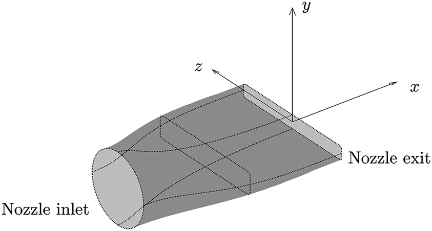


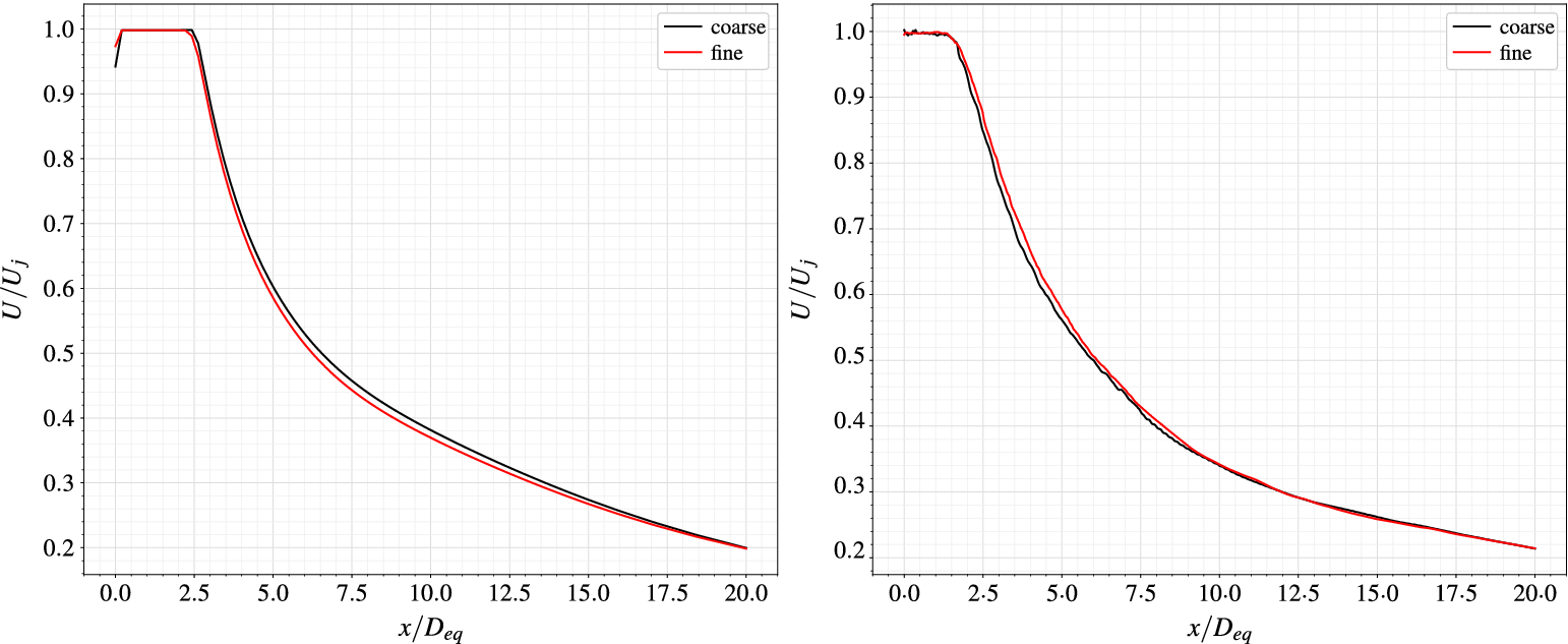





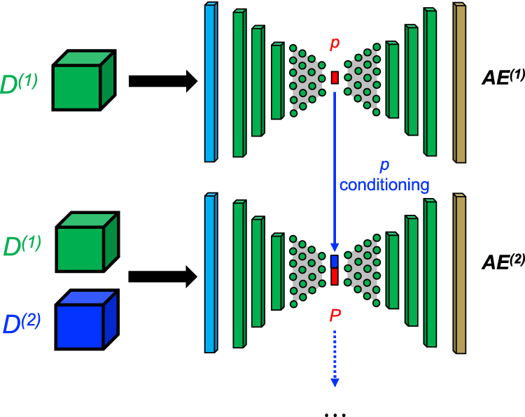

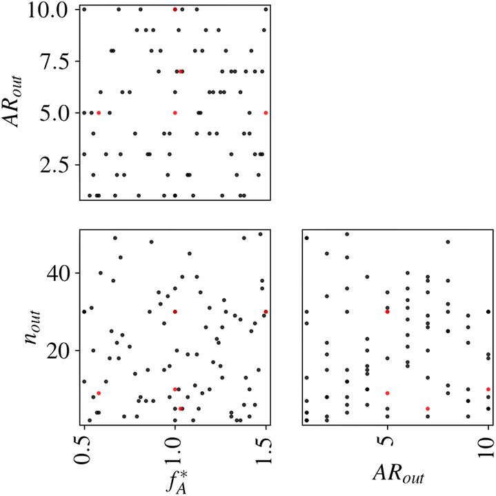
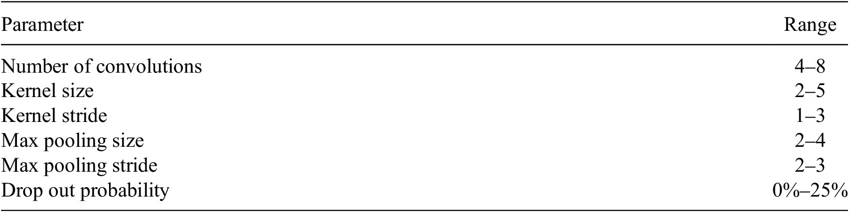
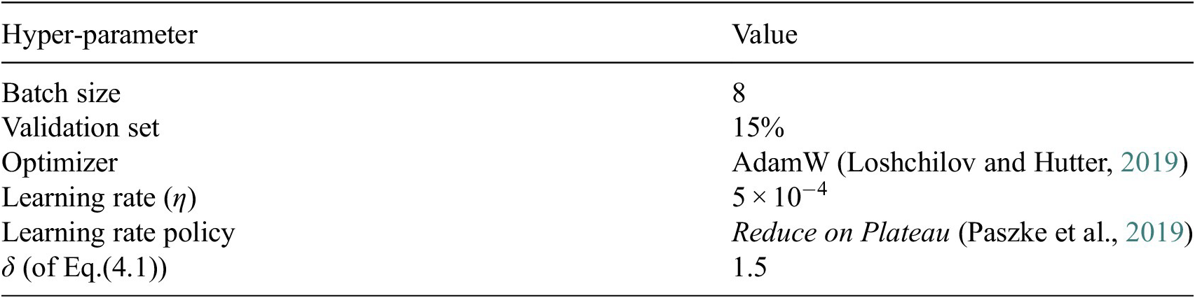
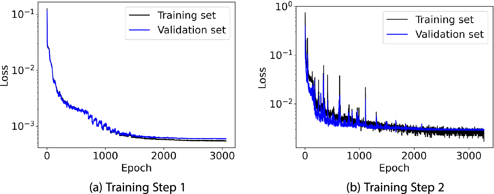


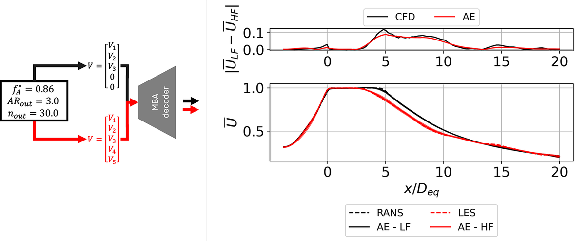


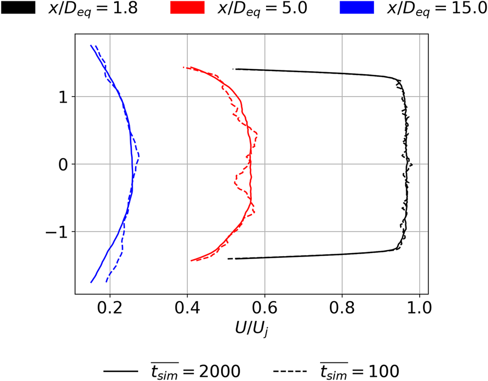








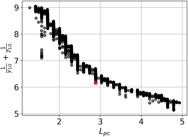


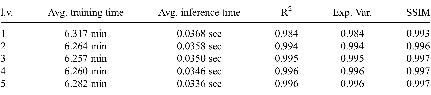




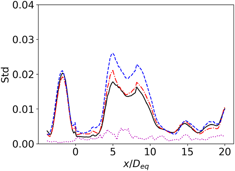











 Open access


Comments
No Comments have been published for this article.