
1 Introduction
The whole ocean–atmosphere system is very sensitive to the processes in the few metres below the water surface. In particular, the top 2.5 m of water column has the same heat capacity as the whole atmosphere above (e.g. Gill Reference Gill1982), while 50 % of the surface-penetrating solar radiation is absorbed within the first 0.5 m of the ocean and 50 % of the breaking surface wave kinetic energy dissipates within 20 % of the significant wave height from the surface (Soloviev & Lucas Reference Soloviev and Lucas2006). Knowledge of the vertical profiles of near-surface currents is of prime importance for modelling horizontal transport of dispersed substances (pollutants, algae, chlorophyll, etc.). Yet another strong motivation for studying the processes linking the ocean surface processes and its interior is that electromagnetic remote sensing of the ocean effectively allows us to see the surface only. Fortunately, the physical processes below produce distinguishable surface signatures which could be deciphered to reveal what is going on beneath. There is a great variety of processes contributing to the formation of the boundary layer in water, ranging from molecular scales to hundreds of kilometres, which include, inter alia, wind, surface gravity and capillary waves and their breaking, air entrainment, surface films, solar heating, shear instabilities, small-scale turbulence, turbulent diffusion of momentum and heat, density stratification suppressing the turbulence, Langmuir circulations, subsurface near-inertial waves; the list is not exhaustive (Soloviev & Lucas Reference Soloviev and Lucas2006; Sullivan & McWilliams Reference Sullivan and McWilliams2010). The Ekman layer plays a prominent role in this list. According to Wang & Huang (Reference Wang and Huang2004) the total global energy input into the Ekman layer is massive – 2.4 TW.
In this work we focus on the fundamentals of a wind generated Ekman boundary layer. The progress in understanding this boundary layer has been slow. It began with the unexpected discovery of Nansen’s polar expedition of 1893–96, that the surface current, and, thus, the drift of the floating ice, was predominantly directed to the right of the wind direction. The first mathematical model of this phenomenon was proposed in the pioneering work by Ekman (Reference Ekman1905). Ekman reduced the effect of wind to tangential stress and, inter alia, derived a steady solution of the Navier–Stokes equations describing forced uniform horizontal motion on the  $f$-plane under the assumption of constant eddy viscosity. Ekman’s classical steady solution predicts the deflection of the surface current due to the Earth’s rotation to be
 $45^{\circ }$ to the right of the wind direction in the Northern hemisphere (
 $45^{\circ }$ to the left in the Southern hemisphere) with the flux integrated over entire depth (‘the Ekman transport’) at ninety degrees to the right/left of wind direction. Ekman (Reference Ekman1905) also analytically described the development of the Ekman boundary layer from rest. Within the framework of this model the complete analytical description of the dynamics of the Ekman current generated by an arbitrarily varying wind was derived in terms of explicit Green’s function by Gonella (Reference Gonella1971). The model was extended to finite depth (Lewis & Belcher Reference Lewis and Belcher2004). An overview by Jenkins & Bye (Reference Jenkins and Bye2006) provides a neat summary of Ekman’s work which has a continuing influence on oceanography. Observations of wind-driven currents showed that indeed the surface velocity vertical structure often exhibits a smooth spiral resembling qualitatively the theoretical Ekman spiral (Price, Weller & Schudlich Reference Price, Weller and Schudlich1987). However, substantial quantitative discrepancies between the predictions of the original Ekman model and observations have been reported. In particular, as pointed by Madsen (Reference Madsen1977), Weber (Reference Weber1981) and Lewis & Belcher (Reference Lewis and Belcher2004), the surface current deflection with respect to wind is usually approximately
 $10{-}30^{\circ }$, i.e. noticeably smaller than the
 $45^{\circ }$ predicted by the steady Ekman solution, while the deflections of currents at relatively small (
 ${\sim}5$–20 m) depths are stronger compared to the classical Ekman solution. It was also noted by Chereskin (Reference Chereskin1995) and Price et al. (Reference Price, Weller and Schudlich1987) that, in contrast to the Ekman model, the current speed decreases with depth more rapidly than the current vector rotates to the right. This mismatch is important since the eddy viscosity is estimated by fitting observations to formulae of either the decay of speed with depth or of the velocity rotation with depth; the estimates obtained in these two ways can differ by an order of magnitude (Weller Reference Weller1981; Price et al. Reference Price, Weller and Schudlich1987; Chereskin Reference Chereskin1995; Lenn Reference Lenn2006). Here, we do not aim at reviewing the observations of Ekman currents summarized in an overview by Price & Sundermever (Reference Price and Sundermeyer1999), we just note that there is an inherent difficulty in extracting the forced Ekman component of the current from observations. Many more observations are needed. Especially lacking are observations of the spatio-temporal dynamics of transient Ekman currents. The overwhelming majority of the observations are provided by point measurements with often insufficient vertical and temporal resolutions. Fortunately, rapidly developing gliders (e.g. Merckelbach, Smeed & Griffiths Reference Merckelbach, Smeed and Griffiths2010) and the maturing remote sensing techniques, such as, multi-frequency high-frequency radars (Teague, Vesecky & Hallock Reference Teague, Vesecky and Hallock2001; Zhang & Zebiak Reference Zhang and Zebiak2002), new generation of acoustic Doppler current profilers (e.g. Guerra & Thomson Reference Guerra and Thomson2017) have the potential to revolutionize the observations of the Ekman currents in the near future.
On the modelling side, since the eddy viscosity parameterizations and, especially, the constant eddy viscosity assumption are a strong oversimplification of a very complicated real picture, there were numerous attempts to improve the Ekman model by choosing better parameterizations of turbulence. To this end a better understanding of turbulence phenomenology in the boundary layer is needed, which in itself is an area of intense ongoing research (see review of experimental studies in Csanady (Reference Csanady2001) and Soloviev & Lucas (Reference Soloviev and Lucas2006)). In the modern large-scale ocean models a range of state of the art turbulence closures is employed: ‘K-profile parametrization’ (Large, McWilliams & Doney Reference Large, McWilliams and Doney1994; Reichl et al. Reference Reichl, Wang, Hara, Ginis and Kukulka2016), ‘generalized ocean turbulence model’ (Umlauf & Burchard Reference Umlauf and Burchard2005; Canuto et al. Reference Canuto, Howard, Cheng, Muller, Leboissetier and Jayne2010). By accounting for stratification, wave breaking and Langmuir circulations, these models reproduce reasonably well the seasonal dynamics of the mixed layer (Kantha & Clayson Reference Kantha and Clayson2004; Harcourt Reference Harcourt2015; Reichl et al. Reference Reichl, Wang, Hara, Ginis and Kukulka2016). These closures are widely used in simulations of global and regional oceanic circulations (e.g. Graham et al. Reference Graham, O’Dea, Holt, Polton, Hewitt, Furner, Guihou, Brereton, Arnold, Wakelin and Castillo Sanchez2018), in the ‘ocean only’ mode or coupled with waves and atmosphere (Lewis et al. Reference Lewis, Castillo Sanchez, Arnold, Fallmann, Saulter, Graham, Bush, Siddorn, Palmer and Lock2018). In the last decade the spatial and temporal resolutions of atmospheric forcing in the models have been significantly improved. Thus, the ocean circulation models begin to capture some features of variability caused by atmospheric forcing at meso-, synoptic and inertial scales. However, the interpretation of the ocean response to, say, wind bursts in observations and numerical models is complicated; it requires, as a prerequisite, a better understanding of such basic processes as the Ekman response, instabilities induced by unsteady wind and associated unsteady mixing occurring in the Ekman layer. The present work does not compete with the advanced numerical models, it aims at re-examining the basic processes by extending the mathematical framework within the Ekman-type models as far as possible and at identifying the intrinsic contradictions of this approach.
For the Ekman-type models the fundamental question of how good are the almost universally adopted Boussinesq eddy viscosity closure and the corresponding parametrization of momentum transfer remains outstanding. This crucial issue has been partially addressed by means of large-eddy simulations of steady Ekman boundary layers by Zikanov, Slinn & Dhanak (Reference Zikanov, Slinn and Dhanak2003). Their work does not simulate surface waves and their breaking, but within the framework of such a simplified setting, it confirms the existence of the wall-like layer below and predicts at what depth the eddy viscosity starts to decrease. Thus, at least for steady regimes it provides a simple depth and latitude dependent parametrization of eddy viscosity which we adopt. Note that the viscosity at the surface and its gradient scale with the friction velocity  $u_{\ast }$ differently, namely, as
 $u_{\ast }^{2}$ and
 $u_{\ast }$. Although for the situations with convection (e.g. nocturnal boundary layers) the eddy viscosity closure fails, here we adopt the eddy viscosity hypothesis and thus a priori exclude the situations with convection. On the theoretical side the attempts to modify the Ekman model aimed to improve its performance, while retaining its elegance and simplicity, have never stopped. Our work, on the one hand, belongs to this line of research, but it ends up revealing its intrinsic contradictions.
Below, we briefly overview the progress in theoretical studies of Ekman layer dynamics with different models of the depth dependence of eddy viscosity. Models with vertical eddy viscosity linearly varying with depth have two major advantages: first, they are underpinned by a transparent physics (linear viscosity leads to a logarithmic boundary layer, which, in a certain range of depths, agrees with available observations (e.g. Csanady Reference Csanady2001); the corresponding reduction of the Navier–Stokes equations can be solved exactly in terms of the Bessel functions (e.g. Madsen Reference Madsen1977; Lewis & Belcher Reference Lewis and Belcher2004). Power-law profiles of eddy viscosity were examined both for finite and infinite depth by Jordan & Baker (Reference Jordan and Baker1980), the steady solutions were expressed in terms of the Bessel functions. An attempt to move away from particular profiles was made by Grisogono (Reference Grisogono1995), who suggested employing the WKB solution assuming slow variation of viscosity with depth; however, in the oceanic boundary layer there is no needed scale separation.
Following the idea first put forward by Huang (Reference Huang1979), the Stokes drift due to surface waves was also taken into account; the resulting Stokes–Ekman model was analysed theoretically (Xu & Bowen Reference Xu and Bowen1994; Lewis & Belcher Reference Lewis and Belcher2004) and numerically by large-eddy simulations (Sullivan & McWilliams Reference Sullivan and McWilliams2010). The effect of the Stokes drift was found to be important, but the existing analysis is based on the restrictive assumptions of independence of time of both the eddy viscosity and the Stokes drift. What happens without these assumptions is one the issues addressed below.
Note that the classical steady Ekman (Reference Ekman1905) solution is unstable with respect to finite wavelength perturbations; linear stability analysis carried out by Leibovich & Lele (Reference Leibovich and Lele1985) on the non-traditional  $f$-plane has identified the critical Reynolds numbers and parameters of the most unstable modes; however, since their analysis is confined to the classical Ekman model with constant eddy viscosity, the same for the basic flow and the small-scale perturbations, it is not clear how relevant the obtained instabilities for realistic situations are. The instability of the near-surface current, occurring when the Stokes drift is taken into account, leads to Langmuir circulations (Craik & Leibovich Reference Craik and Leibovich1976; Sullivan & McWilliams Reference Sullivan and McWilliams2010); their presence changes not only the vertical distribution of eddy viscosity but also leads to its horizontal inhomogeneity. Upon spatial averaging the initially horizontally uniform eddy viscosity becomes anisotropic. This fundamental implication was first examined by Wirth (Reference Wirth2010), who derived an anisotropic generalization of the steady Ekman solution. The potentially important idea of the instability of Ekman currents has not been pursued further. In particular, the instability of transient Ekman currents has not been examined, either for constant or depth- and/or time-dependent eddy viscosity. Throughout this paper we refer to all non-steady currents as ‘transient’. To our knowledge, the legitimate question on whether the relatively slow transient Ekman currents with time scales of
 $O(10^{-5}~\text{s})$ are stable or unstable with respect to much faster perturbations has never been posed. Therefore, it is not clear under what conditions the known solutions for transient and steady Ekman currents can occur in reality or even whether they can occur at all. Here, this gap will also be addressed.
The ability of the existing simple models of Ekman currents to capture the response of the oceanic boundary layer to varying-in-time wind stress was examined by Elipot & Gille (Reference Elipot and Gille2009) by comparing predictions of nine different Ekman-type models (three types of eddy viscosity depth dependence and three forms of boundary conditions at the bottom of the mixed layer aimed to mimic the effect of a stratified layer below) against the Southern Ocean drifter observations carried out within the framework of the ongoing Global Drifter Program (Siedler, Gould & Church Reference Siedler, Gould and Church2001; see also http://www.aoml.noaa.gov/phod/dac/index.php). Some of the tested Ekman-type models proved to be surprisingly successful in describing variability in the drifter data. However, the reasons why the least likely models happened to perform better are not clear; the huge scale of this experiment does not allow one to dismiss these findings as a mere coincidence and calls for further study.
The unifying feature of the existing theoretical developments of the Ekman theory is that they do not take into account time dependence of the eddy viscosity caused by varying wind, which is an obvious oversimplification and stark neglect of a key feature of reality. Here, we extend the Ekman model by considering time- (and depth-) dependent eddy viscosity. The turbulence in the Ekman layer is known to vary with time (e.g. Soloviev & Lucas Reference Soloviev and Lucas2006), it is affected by many physical processes, not fully understood yet. We mention just a few: it depends on wind through the wind-induced shear and waves, primarily through wave breaking, which is sensitive to the instantaneous wind and wave age (e.g. Babanin Reference Babanin2011); the turbulence is affected by solar heating and heat exchange, which might create density stratification and thus suppress the turbulence; it might also be affected by near-inertial waves trapped near the surface (Shrira & Forget Reference Shrira and Forget2015), by convection, etc. Here we do not consider specific mechanisms of turbulence temporal variability and exclude effects of large-scale motions, we focus on how a presumed wind-determined time and depth dependence of eddy viscosity manifests in the dynamics of the resulting Ekman current. We assume that, to leading order, the eddy viscosity at the surface scales as friction velocity squared,  $u_{\ast }^{2}$, while its gradient scales as
 $u_{\ast }$, which is supported by the Zikanov et al. (Reference Zikanov, Slinn and Dhanak2003) large-eddy simulations for steady regimes; for sufficiently slow changes of wind this scaling might capture reality in the absence of density stratification. The present study is confined to the non-stratified ocean. Even if the assumed scaling is not exactly true, we are the first to admit that it is also an oversimplification, still, it is worth exploring the effects due to time-dependent eddy viscosity under this not unreasonable assumption; at the moment we do not have a better alternative. We show that once the eddy viscosity closure and tangential stress parametrization of the wind effect have been adopted, the Ekman equations with viscosity varying both in depth and time admit a broad class of novel exact solutions describing the dynamics of transient Ekman currents. These solutions demonstrate the significance of taking into account the time dependence of the eddy viscosity. This enables us to get a new insight into the vertical and temporal variability of transient Ekman currents and to identify the intrinsic limitations of the current Ekman models.
The paper is organized as follows. First, in § 2 we formulate the mathematical model. In § 3 we derive a novel broad class of exact solutions of the Navier–Stokes equations generalizing the Ekman solutions for the situations with time-and-depth-dependent viscosity; note that the value of viscosity at the surface and its gradient can be independent functions of time. In § 4 we examine two basic scenarios of varying wind: a gradual increase ending up with a plateau and a periodic variation. We demonstrate the importance of taking into account the eddy viscosity time dependence by comparing the obtained transient Ekman currents in a few basic scenarios of evolution with those obtained with the steady eddy viscosity models. We show that the transient Ekman currents described by the exact solutions of the Ekman equations found in § 3 are unstable with respect to small-scale fast perturbations; these instabilities proved to be localized near the surface and are very sensitive to the adopted models of eddy viscosity. The general solution for self-similar distributions of eddy viscosity with the power-law depth dependence and an arbitrary time dependence of the wind is derived in appendix A and discussed in § 5. In § 6 we derive the general solution describing the transient Ekman current response to an arbitrarily varying wind, taking into account a time-dependent Stokes drift and a linear dependence of viscosity on depth. We also show that in this setting a steady Ekman current cannot exist, even under constant wind and even if the instabilities of § 3 do not occur or are ignored. The bulk of the derivation is given in appendix B. In the concluding § 6 we summarize our findings and pose the new questions they generate.
2 The mathematical model
We describe ocean response to varying wind starting with the Navier–Stokes equations for viscous and horizontally uniform flow on the non-traditional  $f$-plane under the Boussinesq approximation (e.g. Phillips Reference Phillips1977; Cushman-Roisin & Beckers Reference Cushman-Roisin and Beckers2007). In the Cartesian frame with
 $\boldsymbol{x}$ directed eastward,
 $\boldsymbol{y}$-northward and
 $\boldsymbol{z}$-downward, with the origin at the unperturbed surface of the ocean, the Reynolds-averaged Navier–Stokes equations for the zonal and meridional velocities
 $u,v$ caused by a time-varying horizontally uniform wind stress
 $\{\unicode[STIX]{x1D70F}_{xz}(0,t)$,
 $\unicode[STIX]{x1D70F}_{yz}(0,t)\}$ take the form
 $$\begin{eqnarray}\displaystyle & \displaystyle \frac{\unicode[STIX]{x2202}u}{\unicode[STIX]{x2202}t}-fv=\frac{1}{\unicode[STIX]{x1D70C}}\frac{\unicode[STIX]{x2202}\unicode[STIX]{x1D70F}_{xz}(z,t)}{\unicode[STIX]{x2202}z}, & \displaystyle\end{eqnarray}$$
 $$\begin{eqnarray}\displaystyle & \displaystyle \frac{\unicode[STIX]{x2202}v}{\unicode[STIX]{x2202}t}+fu=\frac{1}{\unicode[STIX]{x1D70C}}\frac{\unicode[STIX]{x2202}\unicode[STIX]{x1D70F}_{yz}(z,t)}{\unicode[STIX]{x2202}z}, & \displaystyle\end{eqnarray}$$
 $\unicode[STIX]{x1D70C}$ is water density,
 $f=2\unicode[STIX]{x1D6FA}\sin \unicode[STIX]{x1D719}$ is the Coriolis parameter (
 $\unicode[STIX]{x1D6FA}$ and
 $\unicode[STIX]{x1D719}$ are, respectively, the Earth’s rotation frequency and latitude). The Reynolds stresses terms
 $\unicode[STIX]{x1D70F}_{xz}\equiv -\unicode[STIX]{x1D70C}\langle \hat{u} {\hat{w}}\rangle$,
 $\unicode[STIX]{x1D70F}_{yz}\equiv -\unicode[STIX]{x1D70C}\langle \hat{v}{\hat{w}}\rangle$ describe the downward transfer of eastward and northward momentum, here
 $\hat{u}$,
 $\hat{v}$ and
 ${\hat{w}}$ are the
 $x-,y-,z-$ components of turbulent velocities,
 $\langle \cdots \rangle$ means Reynolds’ averaging over turbulent fluctuations. Before the Reynolds averaging, the Navier–Stokes equations on the non-traditional
 $f$-plane, which are our starting point, are nonlinear and contain terms with the horizontal component of the Earth rotation
 $\tilde{f}=\unicode[STIX]{x1D6FA}\cos \unicode[STIX]{x1D719}$, for the horizontally uniform mean flows in which we are interested, the nonlinear terms
 $\boldsymbol{u}\boldsymbol{\cdot }\unicode[STIX]{x1D735}\boldsymbol{u}$ and ‘non-traditional terms’ with
 $\tilde{f}$ vanish identically, while nonlinearity of the fluctuations,
 $\hat{\boldsymbol{u}}\boldsymbol{\cdot }\unicode[STIX]{x1D735}\hat{\boldsymbol{u}}$, and an implicit dependence on
 $\tilde{f}$ are retained in the Reynolds stress terms.
We close the equations for the Reynolds-averaged flow by adopting the commonly used Boussinesq hypothesis, i.e. we assume the Reynolds stresses to be proportional to the mean velocity gradient,  $\unicode[STIX]{x2202}\pmb{u}/\unicode[STIX]{x2202}z$, through a single scalar coefficient, the eddy viscosity
 $\unicode[STIX]{x1D708}_{e}(z,t)$:
 $$\begin{eqnarray}\displaystyle \unicode[STIX]{x1D70C}\unicode[STIX]{x1D708}(z,t)\frac{\unicode[STIX]{x2202}u}{\unicode[STIX]{x2202}z}\equiv \unicode[STIX]{x1D70F}_{xz}\equiv -\unicode[STIX]{x1D70C}\langle \hat{u} {\hat{w}}\rangle ,\quad \unicode[STIX]{x1D70C}\unicode[STIX]{x1D708}(z,t)\frac{\unicode[STIX]{x2202}v}{\unicode[STIX]{x2202}z}\equiv \unicode[STIX]{x1D70F}_{yz}\equiv -\unicode[STIX]{x1D70C}\langle \hat{v}{\hat{w}}\rangle . & & \displaystyle\end{eqnarray}$$
Recall that in our context the use of this closure has been justified in Zikanov et al. (Reference Zikanov, Slinn and Dhanak2003) through extensive large-eddy simulations, although only for steady winds. We can also expect it to be applicable for the time-dependent winds for the time scales exceeding the characteristic scale of the small-scale turbulence adjustment.
Upon adopting the Boussinesq closure (2.2) the momentum equations (2.1) can be written as,
 $$\begin{eqnarray}\frac{\unicode[STIX]{x2202}u}{\unicode[STIX]{x2202}t}-fv=\frac{1}{\unicode[STIX]{x1D70C}}\frac{\unicode[STIX]{x2202}}{\unicode[STIX]{x2202}z}\left(\unicode[STIX]{x1D70C}\unicode[STIX]{x1D708}_{e}(z,t)\frac{\unicode[STIX]{x2202}u}{\unicode[STIX]{x2202}z}\right),\quad \frac{\unicode[STIX]{x2202}v}{\unicode[STIX]{x2202}t}+fu=\frac{1}{\unicode[STIX]{x1D70C}}\frac{\unicode[STIX]{x2202}}{\unicode[STIX]{x2202}z}\left(\unicode[STIX]{x1D70C}\unicode[STIX]{x1D708}_{e}(z,t)\frac{\unicode[STIX]{x2202}v}{\unicode[STIX]{x2202}z}\right).\end{eqnarray}$$
We confine our study to density-uniform flows, which makes the equations above independent of density. Following Ekman (Reference Ekman1905) we introduce a complex horizontal velocity  $\boldsymbol{U}=u+\text{i}v$, which enables us to cast the momentum equations into the following single equation for
 $\boldsymbol{U}(z,t)$,
 $$\begin{eqnarray}\frac{\unicode[STIX]{x2202}\boldsymbol{U}}{\unicode[STIX]{x2202}t}+\text{i}f\boldsymbol{U}=\frac{\unicode[STIX]{x2202}}{\unicode[STIX]{x2202}z}\left(\unicode[STIX]{x1D708}_{e}(z,t)\frac{\unicode[STIX]{x2202}\boldsymbol{U}}{\unicode[STIX]{x2202}z}\right).\end{eqnarray}$$
We stress that this modified Ekman equation represents an exact reduction of the Navier–Stokes equations for the horizontally uniform non-stratified viscous flows on the  $f$-plane with time- and depth-dependent viscosity.
The motion has to satisfy the boundary condition of continuity of the shear stress at the free surface: a horizontally uniform time-dependent wind produces tangential stress  $\pmb{\unicode[STIX]{x1D70F}}(t)$ at the ocean surface, so that in our coordinate frame with the downward
 $\boldsymbol{z}$-axis,
 $$\begin{eqnarray}\displaystyle \left[\unicode[STIX]{x1D708}_{e}(z,t)\frac{\unicode[STIX]{x2202}\boldsymbol{U}}{\unicode[STIX]{x2202}z}\right]_{z=0}=\frac{-\pmb{\unicode[STIX]{x1D70F}}(t)}{\unicode[STIX]{x1D70C}}. & & \displaystyle\end{eqnarray}$$
The velocity should vanish at the bottom  $z=H$, however, throughout this paper, we apply the second boundary condition in the form,
 $$\begin{eqnarray}\frac{\unicode[STIX]{x2202}\boldsymbol{U}}{\unicode[STIX]{x2202}z}\rightarrow 0\quad \text{as }z\rightarrow \infty .\end{eqnarray}$$
Since the effect of friction is confined to the Ekman boundary layer adjacent to the upper surface we, without loss of generality, may apply the lower boundary condition in the form (2.6) to all situations where the fluid depth far exceeds the thickness of the boundary layer.
The initial condition at  $t=0$ is an arbitrary initial distribution
 $\boldsymbol{U}(z,0)$. The generalization of the Ekman model (2.4) with the boundary conditions (2.5) and (2.6) provides the basis of the present study focussed upon elucidating the effects of time- (and depth-) dependent eddy viscosity.
3 Solvable models
As discussed in the introduction, the specific time dependence of the eddy viscosity might depend on a variety of physical mechanisms, not fully understood yet. For an arbitrary  $v_{e}(z,t)$ the only way to proceed is to simulate numerically the initial-value problem (2.4)–(2.6). Since the problem is linear, it is a relatively straightforward numerical task.
In this work we consider the situations that are tractable analytically. In this section, first, we outline certain classes of time- and depth-dependent eddy viscosity distributions which allow exact solutions of the Ekman equations. Then, focussing on the flows with eddy viscosity linearly varying with depth, we assume that the eddy viscosity at the surface scales as  $u_{\ast }^{2}$, while its gradient scales as
 $u_{\ast }$ (
 $u_{\ast }=\sqrt{|\pmb{\unicode[STIX]{x1D70F}}|/\unicode[STIX]{x1D70C}_{water}}$ is the friction velocity in water). Such a link between
 $\unicode[STIX]{x1D708}_{e}$ and
 $u_{\ast }$ has been established for steady non-stratified flows in Zikanov et al. (Reference Zikanov, Slinn and Dhanak2003). Here, we adopt this link, expecting it to hold, at least, for sufficiently slowly varying winds. Where appropriate, we take the constants of proportionality from the simulations of Zikanov et al. (Reference Zikanov, Slinn and Dhanak2003).
3.1 Self-similar eddy viscosity:  $\unicode[STIX]{x1D708}_{e}(z,t)=\unicode[STIX]{x1D708}_{0}\unicode[STIX]{x1D708}_{e1}(t)(1+z/\unicode[STIX]{x1D6FC}(t))^{\unicode[STIX]{x1D707}}$

Consider a class of self-similar parameterizations of eddy viscosity with two arbitrary functions of time  $\unicode[STIX]{x1D708}_{e1}(t)$ and
 $\unicode[STIX]{x1D6FC}(t)$,
 $$\begin{eqnarray}\unicode[STIX]{x1D708}_{e}(z,t)=\unicode[STIX]{x1D708}_{0}\unicode[STIX]{x1D708}_{e1}(t)(1+z/\unicode[STIX]{x1D6FC}(t))^{\unicode[STIX]{x1D707}},\quad (\unicode[STIX]{x1D707}>0,\unicode[STIX]{x1D6FC}>0).\end{eqnarray}$$
The substitution,
 $$\begin{eqnarray}\boldsymbol{U}(z,t)=\text{e}^{-\text{i}ft}\boldsymbol{W}(Z,T),\quad T=\unicode[STIX]{x1D708}_{0}\int _{0}^{t}\unicode[STIX]{x1D708}_{e1}(\unicode[STIX]{x1D709})\,\text{d}\unicode[STIX]{x1D709},\quad Z=1+\frac{z}{\unicode[STIX]{x1D6FC}(t(T))},\quad T_{1}=\int _{0}^{T}\frac{\text{d}\unicode[STIX]{x1D701}}{\unicode[STIX]{x1D6FC}^{2}(t(\unicode[STIX]{x1D701}))},\end{eqnarray}$$
turns the governing equation (2.4) into the following tractable diffusion equation
 $$\begin{eqnarray}\displaystyle \frac{\unicode[STIX]{x2202}\boldsymbol{W}}{\unicode[STIX]{x2202}T_{1}}=\frac{\unicode[STIX]{x2202}}{\unicode[STIX]{x2202}Z}\left[Z^{\unicode[STIX]{x1D707}}\frac{\unicode[STIX]{x2202}\boldsymbol{W}}{\unicode[STIX]{x2202}Z}\right]. & & \displaystyle\end{eqnarray}$$
The boundary conditions at the surface and at infinity and the initial conditions in terms of the new variables take the form
 $$\begin{eqnarray}\displaystyle & \displaystyle \frac{\unicode[STIX]{x2202}\boldsymbol{W}}{\unicode[STIX]{x2202}Z}=\frac{-\text{e}^{\text{i}ft(T_{1})}\unicode[STIX]{x1D749}(t(T_{1}))\unicode[STIX]{x1D6FC}(t(T_{1}))}{\unicode[STIX]{x1D70C}\unicode[STIX]{x1D708}_{e}(z,t(T_{1}))}\equiv \boldsymbol{G}(T_{1})\quad \text{at }Z=1, & \displaystyle\end{eqnarray}$$
 $$\begin{eqnarray}\displaystyle & & \displaystyle \nonumber\\ \displaystyle & \displaystyle \frac{\unicode[STIX]{x2202}\boldsymbol{W}}{\unicode[STIX]{x2202}Z}\rightarrow 0\quad \text{as }Z\rightarrow \infty , & \displaystyle\end{eqnarray}$$
 $$\begin{eqnarray}\displaystyle & \displaystyle \boldsymbol{W}(Z,T_{1})|_{T_{1}=0}=\boldsymbol{U}(z(Z),0).\quad & \displaystyle\end{eqnarray}$$
Details of the derivation and solutions are given in appendix A, a brief discussion of few examples of solutions is given in § 5.
We reiterate that here the eddy viscosity is allowed to depend on two arbitrary functions of time,  $\unicode[STIX]{x1D708}_{e1}(t)$ and
 $\unicode[STIX]{x1D6FC}(t)$.
3.2 Eddy viscosity linearly dependent on depth with Zikanov’s scaling
In this section we focus on the simplest, and, we believe the most relevant for a non-stratified upper ocean, model of the self-similar class of eddy viscosity distributions. Here, we examine a time-dependent eddy viscosity linearly varying with depth employing Zikanov’s scaling,
 $$\begin{eqnarray}\displaystyle \unicode[STIX]{x1D708}_{e}=u_{\ast }^{2}(t)\left(g_{0}+\frac{g_{1}}{u_{\ast }(t)}z\right), & & \displaystyle\end{eqnarray}$$
where  $g_{0}$ and
 $g_{1}$ are latitude-dependent constants specified in accordance with Zikanov’s model, or differently, if we have grounds to do so. We employ ansatz (3.4) rather than the more general form (3.1), since this presentation of eddy viscosity enables us to investigate the case
 $\unicode[STIX]{x1D708}(0)=0$ earlier considered by Madsen (Reference Madsen1977) for constant-in-time viscosity, which is impossible using (3.1). Therefore, we briefly repeat the derivation of the general solution employing (3.4), which proves to be easier than modifying the general results based on (3.1). On substituting (3.4) into the Ekman equation and boundary conditions, we, in contrast to (3.2), retaining the same independent variables, obtain,
 $$\begin{eqnarray}\displaystyle & \displaystyle \frac{\unicode[STIX]{x2202}\boldsymbol{W}}{\unicode[STIX]{x2202}t}=u_{\ast }^{2}(t)\frac{\unicode[STIX]{x2202}}{\unicode[STIX]{x2202}z}\left[g_{0}+\left(\frac{g_{1}}{u_{\ast }(t)}z\right)\frac{\unicode[STIX]{x2202}\boldsymbol{W}}{\unicode[STIX]{x2202}z}\right],\quad \left(\boldsymbol{W}(z,t)=\text{e}^{-\text{i}ft}\boldsymbol{U}(t,z)\right). & \displaystyle\end{eqnarray}$$
 $$\begin{eqnarray}\displaystyle & \displaystyle \frac{\unicode[STIX]{x2202}\boldsymbol{W}}{\unicode[STIX]{x2202}z}=\frac{-\text{e}^{\text{i}ft}\unicode[STIX]{x1D749}(t)}{\unicode[STIX]{x1D70C}\unicode[STIX]{x1D708}_{e}(0,t)}\quad \text{at }z=0, & \displaystyle\end{eqnarray}$$
 $$\begin{eqnarray}\displaystyle & \displaystyle \boldsymbol{W}=0\quad \text{as }z\rightarrow \infty & \displaystyle\end{eqnarray}$$
 $$\begin{eqnarray}\displaystyle & \displaystyle \boldsymbol{W}(z,t)|_{t=0}=\boldsymbol{U}(z,0). & \displaystyle\end{eqnarray}$$
Let
 $$\begin{eqnarray}\tilde{Z}=g_{0}+\frac{g_{1}}{u_{\ast }(t)}z.\end{eqnarray}$$
Since,
 $$\begin{eqnarray}\frac{\unicode[STIX]{x2202}\boldsymbol{W}}{\unicode[STIX]{x2202}z}=\frac{g_{1}}{u_{\ast }(t)}\frac{\unicode[STIX]{x2202}\boldsymbol{W}}{\unicode[STIX]{x2202}\tilde{Z}},\quad \frac{\unicode[STIX]{x2202}^{2}\boldsymbol{W}}{\unicode[STIX]{x2202}z^{2}}=\left(\frac{g_{1}}{u_{\ast }(t)}\right)^{2}\frac{\unicode[STIX]{x2202}^{2}\boldsymbol{W}}{\unicode[STIX]{x2202}\tilde{Z}^{2}},\end{eqnarray}$$
 $$\begin{eqnarray}\displaystyle & \displaystyle \frac{\unicode[STIX]{x2202}\boldsymbol{W}}{\unicode[STIX]{x2202}t}=g_{1}^{2}\frac{\unicode[STIX]{x2202}}{\unicode[STIX]{x2202}\tilde{Z}}\left[\tilde{Z}\frac{\unicode[STIX]{x2202}\boldsymbol{W}}{\unicode[STIX]{x2202}\tilde{Z}}\right] & \displaystyle\end{eqnarray}$$
 $$\begin{eqnarray}\displaystyle & \displaystyle \frac{\unicode[STIX]{x2202}\boldsymbol{W}}{\unicode[STIX]{x2202}\tilde{Z}}=\frac{-\text{e}^{\text{i}ft}\unicode[STIX]{x1D749}(t)}{\unicode[STIX]{x1D70C}g_{1}\,u_{\ast }(t)\tilde{Z}}\quad \text{at }\tilde{Z}=g_{0}, & \displaystyle\end{eqnarray}$$
 $$\begin{eqnarray}\displaystyle & \displaystyle \boldsymbol{W}=0\quad \text{as }\tilde{Z}\rightarrow \infty , & \displaystyle\end{eqnarray}$$
 $$\begin{eqnarray}\displaystyle & \displaystyle \boldsymbol{W}(\tilde{Z},t)|_{t=0}=\boldsymbol{U}(z(\tilde{Z}),0)\quad \left(z(\tilde{Z})=\frac{u_{\ast }}{g_{0}}[\tilde{Z}-g_{0}]\right). & \displaystyle\end{eqnarray}$$
The Laplace transform with respect to  $t$ (
 ${\mathcal{L}}\{\boldsymbol{W}(t)\}\equiv \hat{\boldsymbol{W}}(s)$) of (3.9) yields an equation of the Bessel type,
 $$\begin{eqnarray}\displaystyle g_{1}^{2}\tilde{Z}\frac{\text{d}^{2}\hat{\boldsymbol{W}}}{\text{d}\tilde{Z}^{2}}+g_{1}^{2}\frac{\text{d}\hat{\boldsymbol{W}}}{\text{d}\tilde{Z}}-s\hat{\boldsymbol{W}}=-\boldsymbol{U}(z(\tilde{Z}),0). & & \displaystyle\end{eqnarray}$$
Its general solution is a sum of the general solution of the homogeneous equation,  $\hat{\boldsymbol{W}}_{h}$, and a particular solution of the inhomogeneous equation,
 $\hat{\boldsymbol{W}}_{p}$:
 $$\begin{eqnarray}\displaystyle \hat{\boldsymbol{W}}=\hat{\boldsymbol{W}}_{h}+\hat{\boldsymbol{W}}_{p}, & & \displaystyle\end{eqnarray}$$
where
 $$\begin{eqnarray}\displaystyle \hat{\boldsymbol{W}}_{h}(\tilde{Z},t)=c_{1}\text{I}_{0}\left[\frac{2}{g_{1}}\sqrt{s\tilde{Z}}\right]+c_{2}\text{K}_{0}\left[\frac{2}{g_{1}}\sqrt{s\tilde{Z}}\right], & & \displaystyle\end{eqnarray}$$
and  $\text{I}_{0}[\unicode[STIX]{x1D701}],\text{K}_{0}[\unicode[STIX]{x1D701}]$ are the modified Bessel functions of the first and second kind respectively (e.g. Abramowitz & Stegun Reference Abramowitz and Stegun1972), while
 $c_{1},c_{2}$ are constants specified by the boundary conditions. A particular solution
 $\hat{\boldsymbol{W}}_{p}$ is expressed in terms of the fundamental solutions of the homogeneous equation
 $\text{I}_{0}[\unicode[STIX]{x1D701}]$ and
 $\text{K}_{0}[\unicode[STIX]{x1D701}]$, and the right-hand side of the inhomogeneous equation
 $$\begin{eqnarray}\displaystyle \hat{\boldsymbol{W}}_{p} & = & \displaystyle -\frac{2}{g_{1}^{2}}\text{I}_{0}\left[\frac{2}{g_{1}}\sqrt{s\tilde{Z}}\right]\int _{g_{0}}^{\tilde{Z}}\text{K}_{0}\left[\frac{2}{g_{1}}\sqrt{s\unicode[STIX]{x1D709}}\right]U(z(\unicode[STIX]{x1D709}),0)\,\text{d}\unicode[STIX]{x1D709}\nonumber\\ \displaystyle & & \displaystyle +\,\frac{2}{g_{1}^{2}}\text{K}_{0}\left[\frac{2}{g_{1}}\sqrt{s\tilde{Z}}\right]\int _{g_{0}}^{\tilde{Z}}\text{I}_{0}\left[\frac{2}{g_{1}}\sqrt{s\unicode[STIX]{x1D709}}\right]U(z(\unicode[STIX]{x1D709}),0)\,\text{d}\unicode[STIX]{x1D709}.\end{eqnarray}$$
Hence, the general solution of (3.13) satisfying the initial condition (3.12) takes the form,
 $$\begin{eqnarray}\displaystyle \hat{\boldsymbol{W}} & = & \displaystyle \text{I}_{0}\left[\frac{2}{g_{1}}\sqrt{s\tilde{Z}}\right]\left(c_{1}-\frac{2}{g_{1}^{2}}\int _{g_{0}}^{\tilde{Z}}\text{K}_{0}\left[\frac{2}{g_{1}}\sqrt{s\unicode[STIX]{x1D709}}\right]U(z(\unicode[STIX]{x1D709}),0)\,\text{d}\unicode[STIX]{x1D709}\right)\nonumber\\ \displaystyle & & \displaystyle +\,\text{K}_{0}\left[\frac{2}{g_{1}}\sqrt{s\tilde{Z}}\right]\left(c_{2}+\frac{2}{g_{1}^{2}}\int _{g_{0}}^{\tilde{Z}}\text{I}_{0}\left[\frac{2}{g_{1}}\sqrt{s\unicode[STIX]{x1D709}}\right]U(z(\unicode[STIX]{x1D709}),0)\,\text{d}\unicode[STIX]{x1D709}\right).\end{eqnarray}$$
The unspecified constants  $c_{1},c_{2}$ are determined by applying the boundary conditions. Using the condition at infinity (3.7) we eliminate
 $c_{1}$,
 $$\begin{eqnarray}\displaystyle \hat{\boldsymbol{W}}=\text{K}_{0}\left[\frac{2}{g_{1}}\sqrt{s\tilde{Z}}\right]\left(c_{2}+\frac{2}{g_{1}^{2}}\int _{g_{0}}^{\tilde{Z}}\text{I}_{0}\left[\frac{2}{g_{1}}\sqrt{s\unicode[STIX]{x1D709}}\right]U(z(\unicode[STIX]{x1D709}),0)\,\text{d}\unicode[STIX]{x1D709}\right). & & \displaystyle\end{eqnarray}$$
To find  $c_{2}$ we apply the transformed condition at the surface,
 $$\begin{eqnarray}\frac{\unicode[STIX]{x2202}\hat{\boldsymbol{W}}}{\unicode[STIX]{x2202}Z}|_{\tilde{Z}=g_{0}}={\mathcal{L}}\left\{\frac{-\text{e}^{\text{i}ft}\unicode[STIX]{x1D749}(t)}{\unicode[STIX]{x1D70C}g_{1}u_{\ast }(t)\tilde{Z}}\right\},\end{eqnarray}$$
which yields,
 $$\begin{eqnarray}c_{2}=\frac{\sqrt{g_{0}}}{\sqrt{s}K_{1}\left[\frac{2}{g_{1}}\sqrt{sg_{0}}\right]}\left({\mathcal{L}}\left\{\frac{\text{e}^{\text{i}ft}\unicode[STIX]{x1D749}(t)}{\unicode[STIX]{x1D70C}g_{0}u_{\ast }(t)}\right\}+\frac{2}{g_{1}}\text{I}_{0}\left[\frac{2}{g_{1}}\sqrt{sg_{0}}\right]\text{K}_{0}\left[\frac{2}{g_{1}}\sqrt{sg_{0}}\right]U(z(g_{0}),0)\right)\!.\end{eqnarray}$$
Thus, the general solution of (3.13) satisfying the boundary and initiate conditions is
 $$\begin{eqnarray}\displaystyle \hat{\boldsymbol{W}}(\tilde{Z},t)=\text{K}_{0}\left[\frac{2}{g_{1}}\sqrt{s\tilde{Z}}\right]\left(c_{2}+\frac{2}{g_{1}^{2}}\int _{g_{0}}^{\tilde{Z}}\text{I}_{0}\left[\frac{2}{g_{1}}\sqrt{s\unicode[STIX]{x1D709}}\right]U(z(\unicode[STIX]{x1D709}),0)\,\text{d}\unicode[STIX]{x1D709}\right), & & \displaystyle\end{eqnarray}$$
where  $c_{2}$ is given by (3.19).
The general solution in terms of the original variables  $U(z,t)$,
 $t$ and
 $z$ is obtained by inserting
 $\tilde{Z}=g_{0}+(g_{1}/u_{\ast }(t))z$ into (3.20) and taking the inverse Laplace transform,
 $$\begin{eqnarray}\displaystyle \boldsymbol{U}(z,t)=\text{e}^{-\text{i}ft}\boldsymbol{W}(z,t),\quad \boldsymbol{W}(z,t)=\frac{1}{2\unicode[STIX]{x03C0}i}\int _{c-\text{i}\infty }^{c+\text{i}\infty }\tilde{\boldsymbol{W}}(z,s)\text{e}^{st}\,\text{d}s;\quad c\geqslant 0. & & \displaystyle\end{eqnarray}$$
This is the general solution for a logarithmic boundary layer corresponding to a linear-in-depth time-dependent eddy viscosity, under arbitrarily varying wind and with any initial current profile  $\boldsymbol{U}(z,0)$. The solution can be simplified for particular cases of interest considered below.
3.3 Particular cases
3.3.1 ‘Time-dependent Madsen model’ ($g_{0}=0$)

Consider a particular case when  $g_{0}=0$, as the simplest model where we encounter effects due to both the depth and time dependences of eddy viscosity. Whether such a model can capture reality better than a constant-in-time eddy viscosity is an open question. Madsen (Reference Madsen1977) put forward a model with a linearly growing with depth and constant in time eddy viscosity. For simplicity only, we confine our attention to motions starting from rest, i.e. we assume
 $\boldsymbol{U}(z,0)=0$. Here, we do not adhere to the Zikanov’s scaling of the eddy viscosity and present the eddy viscosity as
 $\unicode[STIX]{x1D708}_{e}=\unicode[STIX]{x1D708}_{e1}(t)g_{1}z$, where
 $\unicode[STIX]{x1D708}_{e1}(t)$ is an arbitrary function of time (not necessarily
 $u_{\ast }(t)$), while
 $g_{1}$ is kept constant. Then,
 $$\begin{eqnarray}\boldsymbol{U}(z,t)=\text{e}^{-\text{i}ft}\boldsymbol{W}(z,T),\quad \boldsymbol{W}(z,T)=\frac{1}{g_{1}}\frac{\text{e}^{\text{i}ft(T)}\unicode[STIX]{x1D749}(t(T))}{\unicode[STIX]{x1D70C}\unicode[STIX]{x1D708}_{e1}(t(T))}\ast _{(T)}\frac{1}{T}\text{e}^{-z/g_{1}T},\quad T=\int _{0}^{t}\unicode[STIX]{x1D708}_{e1}(\unicode[STIX]{x1D709})\,\text{d}\unicode[STIX]{x1D709},\end{eqnarray}$$
where  $\unicode[STIX]{x1D6F6}\ast _{(T)}\unicode[STIX]{x1D6F9}$ is the convolution of functions
 $\unicode[STIX]{x1D6F6}$ and
 $\unicode[STIX]{x1D6F9}$ with respect to
 $T$,
 $$\begin{eqnarray}\unicode[STIX]{x1D6F6}\ast _{(T)}\unicode[STIX]{x1D6F9}=\int _{0}^{T}\unicode[STIX]{x1D6F6}(T-\unicode[STIX]{x1D709})\unicode[STIX]{x1D6F9}(\unicode[STIX]{x1D709})\,\text{d}\unicode[STIX]{x1D709}.\end{eqnarray}$$
For constant  $\unicode[STIX]{x1D708}_{e1}$ the solution (3.22) reduces to that of Madsen (Reference Madsen1977).
3.3.2 Time-dependent uniform viscosity ($g_{1}=0$)

This is the most direct generalization of the Ekman model with varying-in-time depth-independent viscosity. In this case, it is easier to get the solution directly from the basic equations than from the general solution (3.21). Applying the Laplace transform in  $T$ to the Ekman equation and boundary conditions (2.4)–(2.6), and, for ultimate simplicity, assuming
 $\boldsymbol{U}(z,0)=0$, we find the general solution in the form
 $$\begin{eqnarray}\displaystyle \boldsymbol{U}(z,t)=\text{e}^{-\text{i}ft}W(T,z);\quad T=\int _{0}^{t}\unicode[STIX]{x1D708}_{e1}(\unicode[STIX]{x1D709})\,\text{d}\unicode[STIX]{x1D709}, & & \displaystyle\end{eqnarray}$$
where
 $$\begin{eqnarray}\displaystyle \boldsymbol{W}(z,T)=\frac{\text{e}^{\text{i}ft(T)}\unicode[STIX]{x1D749}(t(T))}{\unicode[STIX]{x1D70C}\unicode[STIX]{x1D708}_{e1}(t(T))}\ast _{(T)}\frac{\text{e}^{-z^{2}/4T}}{\sqrt{\unicode[STIX]{x03C0}T}}. & & \displaystyle\end{eqnarray}$$
The obtained solution (3.23) describes a time-dependent Ekman current in terms of Green’s function for an infinitely deep homogeneous ocean when the eddy viscosity varies with time only. When  $\unicode[STIX]{x1D708}_{e1}$ is constant, the solution coincides with the Ekman solution.
4 Basic scenarios of the Ekman current response to varying wind
In this section, to elucidate the effect of the time dependence of the eddy viscosity we examine the basic scenarios of the ocean response to the varying wind within the framework of models with eddy viscosity linearly varying with depth (3.4)–(3.8). We consider two basic scenarios of varying wind (all others can be viewed just as combinations of these two): (i) an increase or turn of wind ending up with a plateau, and, (ii) a periodic wind. We examine the Ekman current response in each of these scenarios within the framework of the system (3.4)–(3.8) and compare these predictions with those obtained assuming constant-in-time eddy viscosity.
4.1 Periodic wind
First, consider ocean response to an idealized breeze; a strictly sinusoidal unidirectional wind with diurnal period,
 $$\begin{eqnarray}\displaystyle \mathit{U}_{10}=\mathit{U}_{10}^{0}\sin (\unicode[STIX]{x1D6FA}t),\quad \unicode[STIX]{x1D70F}(t)= & \unicode[STIX]{x1D70F}_{0}H(t)\,\text{Sin}(\unicode[STIX]{x1D6FA}t)|\text{Sin}(\unicode[STIX]{x1D6FA}t)|, & \displaystyle\end{eqnarray}$$
where  $\unicode[STIX]{x1D70F}_{0}=\unicode[STIX]{x1D70C}_{a}C_{D}|\mathit{U}_{10}^{0}|^{2}$,
 $\unicode[STIX]{x1D70C}_{a}=1.25~\text{kg}~\text{m}^{-3}$ is the air density,
 $C_{D}$ is the drag coefficient taken to be
 $1.4\times 10^{-3}$,
 $H(t)$ is the Heaviside function,
 $\unicode[STIX]{x1D6FA}$ is the diurnal frequency and
 $U_{10}$ is the wind velocity at 10 m above the still water level,
 $U_{10}^{0}$ is the amplitude of wind oscillations. In this section
 $\unicode[STIX]{x1D708}_{e}(z,t)$ is
 $\unicode[STIX]{x1D708}_{e}(z,t)=\unicode[STIX]{x1D708}_{e1}(t)[g_{0}+g_{1}z]$ and by virtue of (2.5)
 $\unicode[STIX]{x1D708}_{e}(0,t)\unicode[STIX]{x2202}_{z}\boldsymbol{U}|_{z=0}=-\pmb{\unicode[STIX]{x1D70F}}(t)/\unicode[STIX]{x1D70C}$.
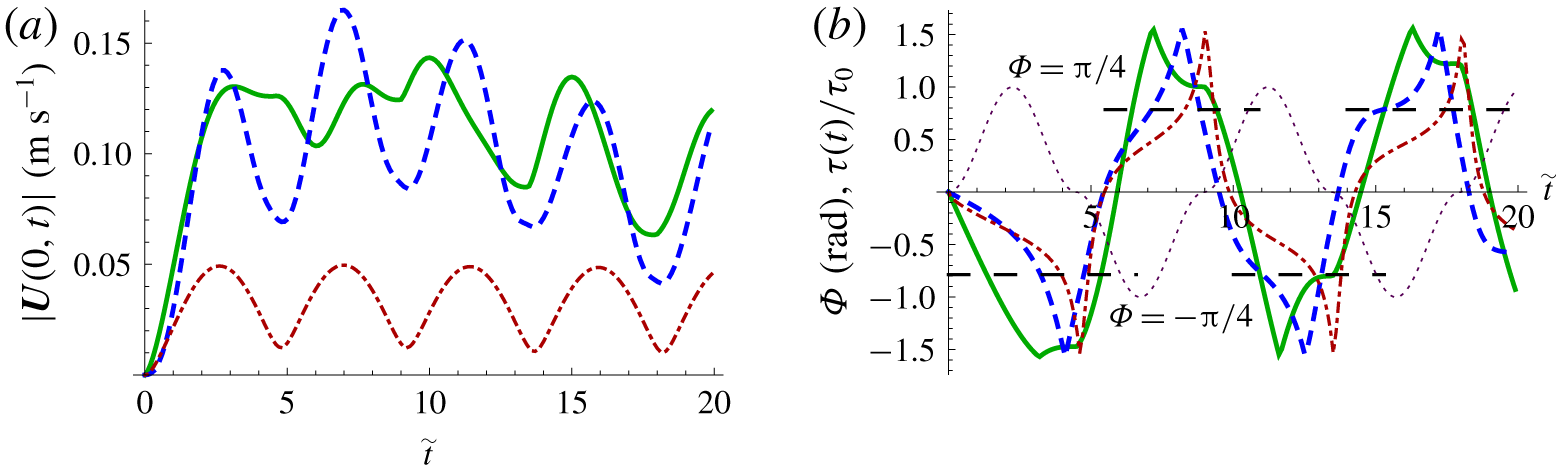
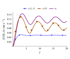
Evolution of surface Ekman currents from rest under a suddenly turned-on periodic wind in three different models of eddy viscosity: the simplified time–depth-dependent viscosity model,  $\unicode[STIX]{x1D708}_{e}=az\cdot \unicode[STIX]{x1D708}_{e1}(t)(\unicode[STIX]{x1D708}_{e1}(0)=1),$ (dot-dashed line, red online); the time-dependent viscosity model,
 $\unicode[STIX]{x1D708}_{e}=0.0125u_{\ast }^{2}/f\cdot \unicode[STIX]{x1D708}_{e1}(t)$ with
 $\unicode[STIX]{x1D708}_{e1}(0)=1$ (solid line, green online); the Ekman solution with constant eddy viscosity
 $\unicode[STIX]{x1D708}_{e}=\unicode[STIX]{x1D708}_{0}$ is plotted by dashed line (blue online). (a) Current speed at the surface
 $|\boldsymbol{U}(0,t)|$ (taken at depth
 $z=0.1~\text{m}$) as function of time (
 $\tilde{t}=ft$). (b) The deflection angle
 $\unicode[STIX]{x1D6F7}(t)$ between the surface current vector (taken at depth
 $z=0.1~\text{m}$) and the wind as function of time. Normalized tangential stress
 $\unicode[STIX]{x1D70F}(t)/\unicode[STIX]{x1D70F}_{0}$ is plotted by dotted line (purple online). The parameter values are:
 $f=10^{-4}~\text{s}^{-1}$,
 $\unicode[STIX]{x1D6FA}=0.7f\,\text{rad}~\text{s}^{-1}$,
 $\unicode[STIX]{x1D708}_{0}\approx 2\times 10^{-2}~\text{m}^{2}~\text{s}^{-1}$,
 $g_{1}=2\times 10^{-2}~\text{m}~\text{s}^{-1}$,
 $\unicode[STIX]{x1D70C}=1027~\text{kg}~\text{m}^{-3}$,
 $\unicode[STIX]{x1D70F}_{0}=0.175~\text{N}~\text{m}^{-2}$,
 $|U_{10}^{0}|=10~\text{m}~\text{s}^{-1}$.

4.1.1 Dynamics of the Ekman current at the surface
Figure 1 shows an example of the evolution of a mid-latitude Ekman current at the ocean surface under a periodic unidirectional wind (4.1) for two models with time-dependent eddy viscosity (with and without linear depth dependence) as well as for the classical Ekman model with constant viscosity as a reference. More specifically, the first model is a simplified version of the general model of § 3 with linear depth dependence, a time-dependent Madsen model,  $\unicode[STIX]{x1D708}_{e}=g_{1}z\cdot \unicode[STIX]{x1D708}_{e1}(t)$, where
 $g_{1}=2\times 10^{-2}~\text{m}~\text{s}^{-1}$. In the second model where viscosity depends only on time, we adopt Zikanov’s scaling for
 $\unicode[STIX]{x1D708}_{e}$:
 $\unicode[STIX]{x1D708}_{e}=0.025/2(u_{\ast }^{2}/f)\cdot \unicode[STIX]{x1D708}_{e1}(t)$, where
 $\unicode[STIX]{x1D708}_{e1}(0)=1$. The constant viscosity
 $\unicode[STIX]{x1D708}_{0}$ is chosen to be
 $2\times 10^{-2}~\text{m}^{2}~\text{s}^{-1}$. Here, and, for consistency in all subsequent figures, to avoid possible singularity at the surface, we take the current at depth 0.1 m as the ‘surface current’. There are noticeable discrepancies between the predictions of all three models, which fact, in our view, shows the importance of a proper accounting for both the time and depth dependence of the eddy viscosity. Obviously, the discrepancies depend on the specific choice of parameters employed in drawing figure 1. At present we are not prepared to speculate on how representative this particular choice is, to this end a systematic analysis of the parameter space is needed, which requires a dedicated work.
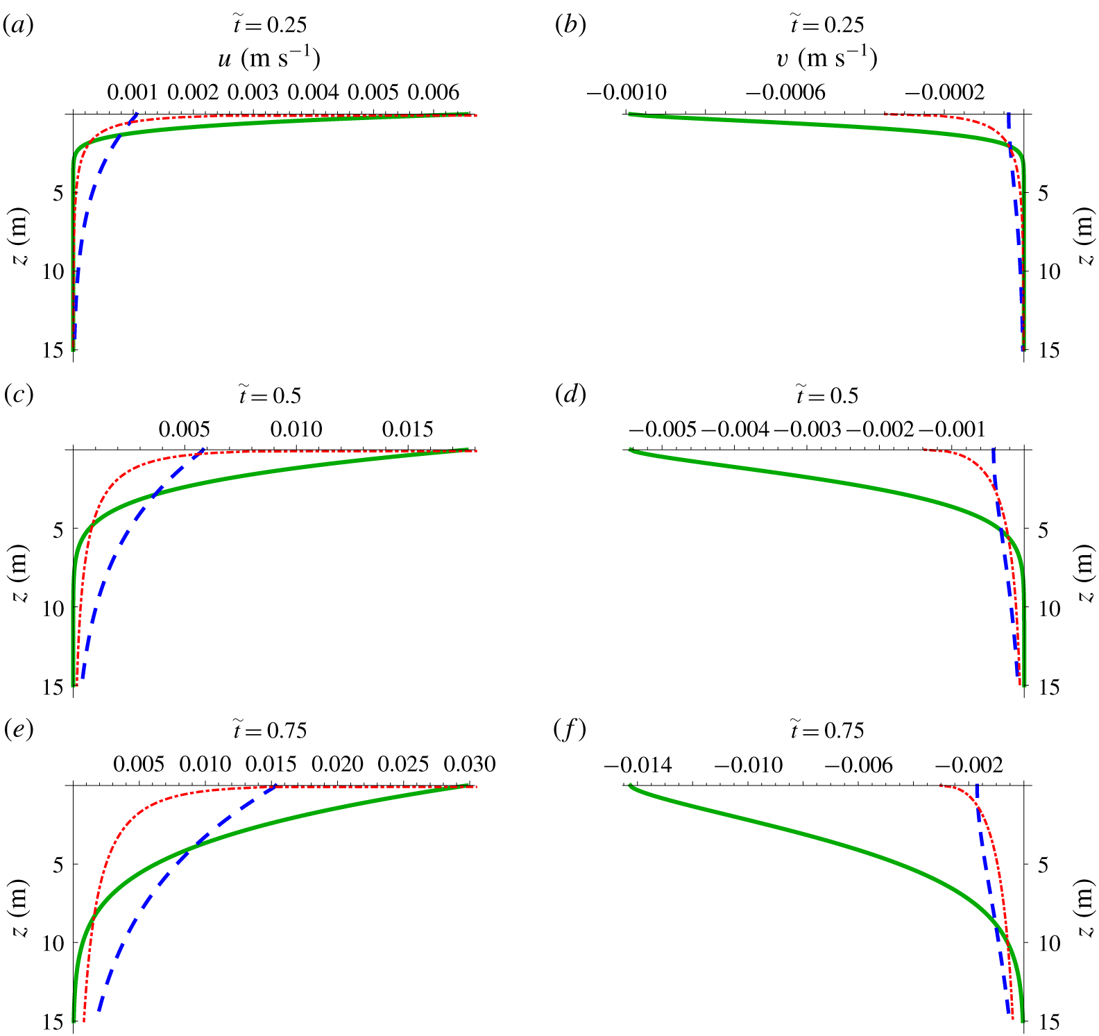
Vertical profiles of the  $x$ and
 $y$ velocity components generated by a suddenly turned-on periodic wind plotted at three sample moments for three different models of figure 1: time–depth-dependent viscosity model (dot-dashed line, red online), the time-dependent viscosity model (solid line, green online), the solution for the classical Ekman model, i.e. with constant eddy viscosity, is plotted by dashed line (blue online). The parameters and expressions for eddy viscosity are the same as in figure 1.

For the chosen set of mid-range parameters the time-dependent Madsen model accounting for both the time and depth dependence of viscosity predicts the strongest variation of the surface current magnitude and the sharpest turns of its direction with respect to wind. This is not surprising given the vanishing viscosity at the surface. The complementary figure 2 illustrates the evolution of both components of the velocity as a function of  $z$, it shows a high degree of subsurface confinement of the surface flow in this case. Thus, when the motion is primarily localized in a very thin layer of fluid, it is natural to expect for the same tangential stress to result in higher velocities and sharper turns. We would ascribe this feature to an artefact of the time-dependent Madsen model; taking into account non-zero
 $\unicode[STIX]{x1D708}_{0}$ comparable to the value in the constant viscosity model would have decreased the amplitude of the surface velocity oscillations and would have smoothed them as well. Note a salient feature of the Ekman response: most of the time the surface current is directed windward, in contrast to the steady Ekman response characterized by a significant deflection (
 $\unicode[STIX]{x03C0}/4$ in the classical Ekman model). Overall, the Ekman currents generated by periodic wind (in all models) show very little resemblance to the steady solutions, although the diurnal period is not small and, a priori, an adiabatic quasi-steady evolution of the Ekman layer might have been considered as a possibility. The characteristic time scale of transition to the steady solution is several inertial periods.

4.1.2 Vertical profiles of the transient Ekman currents caused by periodic breeze
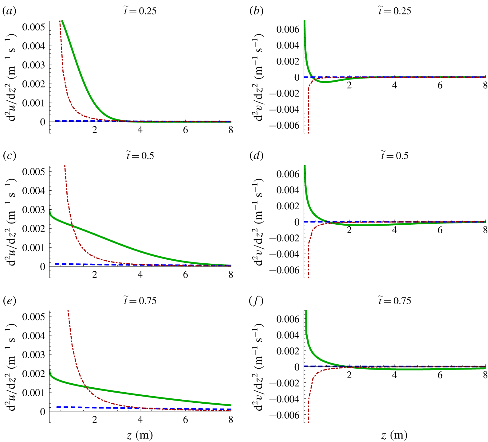
The discrepancies between the predictions of all three models are not confined to the ocean surface, the most profound differences occur below. To give an idea of the flow evolution we draw in figures 2 and 3 instantaneous profiles of the current and its second derivatives sampled at three consecutive moments ( $\tilde{t}=0.25,0.5,0.75$). All three models show a gradual increase of the Ekman current and its slow rotation. Figure 2 shows that the rates of flow acceleration, the rotation of the current direction and the thickness of the boundary layer all differ substantially in the three models. The salient common feature of these transient velocity profiles is the absence of the vertical spiral typical of the steady Ekman currents. The difference between the predictions of the three models is most apparent in the profiles of the second derivatives shown in figure 3.
4.1.3 Instability of the transient Ekman currents caused by periodic wind
With time the evolving current profiles invariably exhibit inflection points and, therefore, by virtue of the Rayleigh criterion, might become linearly unstable. The emergence of inflection points in the current profiles  $u(z,t)$ and
 $v(z,t)$ is illustrated in figure 3. At the sampled moments the profiles predicted by the model with time-dependent eddy viscosity do exhibit a change of curvature sign for all sampled moments, which suggests a possibility of strong, essentially inviscid, inflectional instability, while in the time-dependent Madsen model inflection points develop only at somewhat later times not illustrated by the figure. The occurrence of inflection points in a flow does not in itself necessarily imply the existence and importance of instabilities, but it certainly warrants a study of instabilities of the flow.
First, we specify in what sense it is justified to discuss instability of time-dependent aperiodic flows. The transient Ekman currents we are considering are functions of  $z$ and
 $t$. Their characteristic time scale, as suggested by figure 1, is
 $O(1/f)$. Therefore, assuming separation of scales, we can examine linear instabilities in an adiabatic approximation, that is choosing for analysis particular sample moments
 $t_{s}$ and acting as if the Ekman current were frozen. Such an approach is justified if there exist instabilities with the growth rates
 $\text{Im}\unicode[STIX]{x1D714}$ far exceeding the characteristic inverse time scales of the transient Ekman current, that is with
 $\text{Im}\unicode[STIX]{x1D714}\gg f$. The justification is provided a posteriori, by first examining the corresponding boundary value problem for the perturbations on the transient Ekman current frozen at a chosen sequence of sample moments. If at a chosen sample moment of time
 $t_{s}$ there are sufficiently strong instabilities, we can indeed ignore the dynamics of the corresponding transient Ekman current itself and conclude that such a current cannot exist in reality. If at
 $t=t_{s}$ and at the moments of the previous samplings there are no strong instabilities, we can expect that our solutions describing transient Ekman currents can faithfully predict their dynamics, at least up to this moment.
Now consider the dynamics of a small three-dimensional perturbation  $\{\tilde{u} (z,t),\tilde{v}(z,t),\tilde{w}(z,t)\}$ on a given transient Ekman current
 $\{u(z,t),v(z,t)\}$, assumed frozen at a chosen moment
 $t=t_{s}$. The smallness of the perturbation enables us to linearize the Navier–Stokes equations around the Ekman current, which is horizontally uniform by definition. This fact allows us to perform the Fourier transform with respect to the horizontal coordinates and, by virtue of the assumed scale separation, with respect to time as well. These assumption lead to the boundary value problem for each spectral component similar to that in Leibovich & Lele (Reference Leibovich and Lele1985). Since we are interested only in the fast perturbations we neglect the terms due to rotation, then the standard boundary value problem for the eigenmodes reduces to the Orr–Sommerfield-type equation for the Fourier amplitude of each spectral component with the no-flux and no-stress boundary conditions at the surface and vanishing of the perturbations at infinity. The fundamental weakness of the analysis by Leibovich & Lele (Reference Leibovich and Lele1985), to our knowledge so far not discussed in the literature, is that nothing is known about the small-scale scale-dependent eddy viscosity affecting the perturbations under consideration. Without any discussion Leibovich & Lele (Reference Leibovich and Lele1985) adopt the same value of the constant eddy viscosity for the perturbations as that used for the basic Ekman current. The small-scale viscosity could be orders of magnitude smaller. The boundary value problem based on the Orr–Sommerfield-type equation shares the same fundamental predicament as well. However, although we do not know the small-scale viscosity we can expect the dynamics of the small-scale three-dimensional perturbations to be essentially inviscid, because of the absence of the no-slip boundary condition at the surface. Therefore, to leading order in inverse Reynolds number we can neglect the term due to viscosity and consider instead, of the Orr–Sommerfield-type equation, the Rayleigh equation with the appropriate boundary conditions. Although we do not know the true Reynolds number for the perturbations, for our purposes it is sufficient that it is large. For generic parallel inviscid shear flows the occurrence of one or more inflection points is only the necessary condition for instability, however for boundary-layer-type profiles it is both necessary and sufficient (Tollmien Reference Tollmien1935).
In the inviscid setting the boundary value problem formulated in terms of the perturbation vertical velocity component  $\hat{\tilde{w}}(z,k_{x},k_{y})$ takes the form,
 $$\begin{eqnarray}(\unicode[STIX]{x1D714}-\boldsymbol{k}\boldsymbol{\cdot }\boldsymbol{u}(z))(\unicode[STIX]{x2202}_{zz}^{2}-\boldsymbol{k}^{2})\hat{\tilde{w}}+(\unicode[STIX]{x2202}_{zz}^{2}\boldsymbol{k}\boldsymbol{\cdot }\boldsymbol{u}(z))\hat{\tilde{w}}(z)=0\quad \hat{\tilde{w}}(0)=\hat{\tilde{w}}(\infty )=0,\end{eqnarray}$$
where  $\hat{\tilde{w}}(z,k_{x},k_{y})$ is the eigenmode of the Fourier harmonic with wavevector
 $\{k_{x},k_{y}\}$,
 $\unicode[STIX]{x1D714}(\boldsymbol{k})$ being the eigenvalue. Other notations are standard:
 $\boldsymbol{k}=\{k_{x},k_{y}\}$,
 $\boldsymbol{u}=\{u(z),v(z)\}$. Note that although
 $\boldsymbol{u}(z)$ is specified by two functions
 $u(z),v(z)$, for any chosen
 $\boldsymbol{k}$ the boundary value problem (4.2) is one-dimensional, albeit different for each
 $\boldsymbol{k}$.
The characteristics of the instabilities are obtained by solving numerically the above boundary value problem for each instant of time and each possible wavevector; this has to be repeated for each model of eddy viscosity. Although the eddy viscosity does not enter the boundary value problem (4.2), it strongly affects the Ekman current. On solving the boundary value problem at a chosen instant, we select the eigenvalues with the maximal growth rates. A systematic analysis of these instabilities is a massive time and computer intensive task which requires a dedicated work. When such inviscid instabilities have high growth rates, we can expect almost instant (compared to the inertial time scale) development of larger vortices in the already turbulent flow. Here, we confine ourselves to a very limited study based on analysis of a few examples of transient Ekman currents used in drawing figures 1–3. We aim at addressing just the most basic questions about these instabilities:
(i) Are the instabilities sensitive to the employed viscosity model?
(ii) What are the most unstable characteristic scales of the perturbations and how fast do they grow?
(iii) What are the directions of the wavevectors of the most unstable perturbations?
(iv) How important are the instabilities for the evolution of Ekman currents?
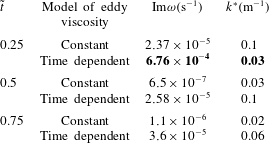
The answers could be deduced from the results of our preliminary numerical study of the boundary value problem (4.2) which are summarized in table 1, where the maximal growth rates  $\text{Im}\unicode[STIX]{x1D714}$ and the corresponding wavenumber
 $k^{\ast }$ are given.
Parameters of short-scale instabilities of transient Ekman currents generated by a suddenly turned-on periodic wind simulated with three different eddy viscosity models employed in drawing figures 1–3. The maximal growth rates of the instabilities  $\text{Im}\unicode[STIX]{x1D714}$ and the corresponding wavenumber
 $k^{\ast }$ are found by solving the boundary value problem (4.2) for the samples of the instantaneous current profiles shown in figures 2 and 3. The parameters of the ‘true instabilities’ which grow much faster than the basic Ekman current are shown in bold. The Ekman currents in the time-dependent Madsen model are stable at the sampled moments and, correspondingly, produce no entries for the table.

First, it is easy to see that the instabilities are very sensitive to the eddy viscosity model: the profiles obtained with the time-dependent Madsen model proved to be stable (for the sampled moments). In accordance with our criterion ( $\text{Im}\unicode[STIX]{x1D714}\gg f$), only the instability occurring at
 $\tilde{t}=0.25$ in the model with the time-dependent viscosity is a true instability, that is it evolves much faster than the characteristic time scale of the unperturbed Ekman current. For the chosen set of parameters all other ‘instabilities’ shown in the table can be ignored as too slow to have a noticeable effect, but it is important to remember that these ignored instabilities exist and a minor tweak of the parameters can strongly increase their growth rates and make these sleeping instabilities actual. It should be also noted that even weak instabilities might have an order-one integral effect on the basic flow if a sufficiently broad range of scales is excited. For the examined sample profiles the most unstable perturbations (both the true and ‘sleeping’ ones) are propagating perpendicular to the wind and have characteristic wavelengths of the order of a hundred metres. The fact that in the example at hand the model with time-dependent viscosity yields at
 $\tilde{t}=0.25$ growth time scales which are much faster than the characteristic time scale of the unperturbed motion, suggests that the instability might completely change the evolution predicted by the exact solutions of the Ekman equations. The current might evolve into something not even remotely resembling the transient Ekman currents our solution predicts. We have not seen such a possibility discussed in the literature so far. To predict what might happen in reality a direct numerical simulation study is needed.
In our sample simulations the instabilities in the classical Ekman model, i.e. with the eddy viscosity constant in time and depth, proved to be very weak, below the threshold of significance. This could justify their neglect when we are interested in time scales of the order of up to a day; time scales exceeding several days require a more comprehensive consideration.
The spatial scales of all found instabilities (both the true and ‘sleeping’ ones) proved to be much larger than the characteristic thickness  $d$ of the boundary layer illustrated in figure 2. This enables us to treat the boundary value problem (4.2) analytically making use of this disparity of scales. A detailed asymptotic derivation of the solution of (4.2) exploiting the smallness of the thickness-to-wavelength ratio can be found in Healey (Reference Healey2017). In particular, the solution provides both the real and imaginary parts of the eigenvalue. Thus, for each perturbation wavevector
 $\boldsymbol{k}$ the growth rates can be found explicitly, then the wavevectors with the fastest growth could be identified. On this basis the judgement can be made on how unstable a particular transient Ekman current is at each particular moment and when this instability should be taken into account. However, even with an analytic solution available a systematic analysis of the instability parameter space represents a massive task and will be a subject of a dedicated follow-up study.
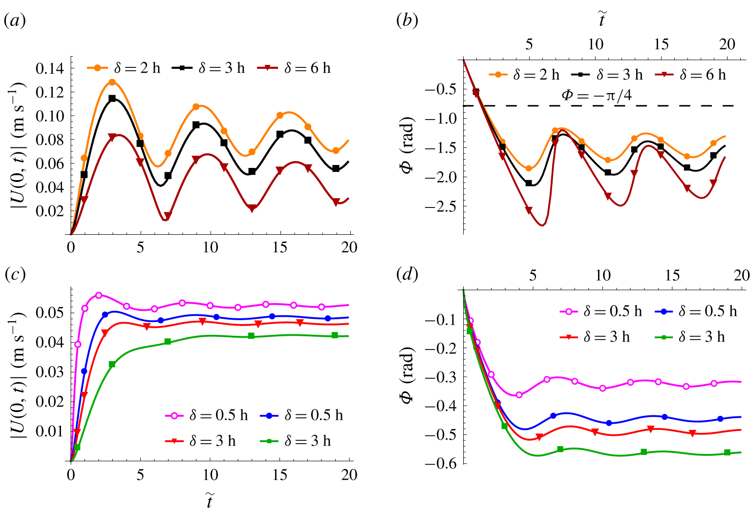
Evolution of Ekman currents under growing wind with different wind growth time scales  $\unicode[STIX]{x1D6FF}$. The magnitude of the current surface velocity
 $|U(0,t)|$ and the angle
 $\unicode[STIX]{x1D6F7}$ of its deflection relative to the wind: (a,b) for the time-dependent vertically uniform viscosity model, (c,d) for the time-dependent Madsen model of viscosity. The surface velocity is taken at
 $z=0.1~\text{m}$. The parameters are the same as in figure 1.

4.2 An increase of wind ending up with a plateau
Consider a gradual increase of unidirectional wind ending up with a plateau with the surface shear stress prescribed in the form,
 $$\begin{eqnarray}\displaystyle U_{10}=\mathit{U}_{10}^{0}\left(1-\text{e}^{-t/\unicode[STIX]{x1D6FF}}\right),\quad \unicode[STIX]{x1D70F}(t)=\unicode[STIX]{x1D70F}_{0}H(t)\left(1-\text{e}^{-t/\unicode[STIX]{x1D6FF}}\right)^{2}. & & \displaystyle\end{eqnarray}$$
By playing with several time dependencies of a gradual increase of wind it was found that the specific function describing the increase is not particularly important and, therefore, in the example we analyse here its functional form was chosen primarily for the sake of convenience. The characteristic time scale of wind increase, on the contrary, proved to be essential; we specify it by a dimensional parameter  $\unicode[STIX]{x1D6FF}$. A few examples of the evolution of Ekman currents in the deep ocean caused by a gradual increase of wind are shown in figures 4 and 5. In figure 4 the evolution of the Ekman currents is plotted for several values of the wind time scale
 $\unicode[STIX]{x1D6FF}$ for the time-dependent Madsen model of viscosity and the model with vertically uniform viscosity dependent only on time. This figure illustrates the evolution of the surface currents (the magnitude and direction). Although the general pattern of the evolution is qualitatively similar in all cases: with an increase of wind the magnitude of the surface current also increases with the same time scale, while its direction is being deflected to the right; an increase of the current is followed by inertial oscillations. The figure demonstrates the sensitivity of the response both to the time scale of the wind increase
 $\unicode[STIX]{x1D6FF}$ and the choice of the viscosity model. While the magnitude of the surface current increases noticeably with the decrease of
 $\unicode[STIX]{x1D6FF}$, the smaller is
 $\unicode[STIX]{x1D6FF}$, the earlier and higher is the ‘saturation’ plateau in
 $|\boldsymbol{U}(0,t)|$, the current orientation with respect to the wind proved to be the most sensitive to
 $\unicode[STIX]{x1D6FF}$, the surface velocity deflection is the smallest for the fastest growth of wind. A possible interpretation is that the rotation of the current vector makes the flow acceleration by wind less effective and thus curtails the growth of its magnitude. The rotation of the current vector is, at least partly, due to the excitation of inertial oscillations. Overall, the surface current direction proved to be the most sensitive characteristic.
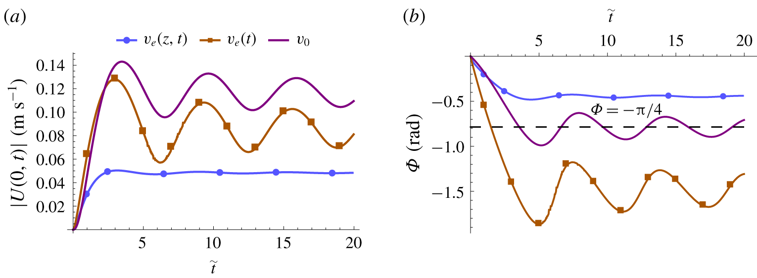
Figure 5 illustrates the role of the viscosity model in the Ekman response to the same wind increase pattern. Three models of eddy viscosity are considered: time-dependent Madsen model, model with vertically uniform time-dependent viscosity and the model with constant viscosity. The increase of the surface current is always followed by inertial oscillations which are most pronounced for the model with eddy viscosity dependent on time only, and the least pronounced for the time-dependent Madsen model. The amplitude of the oscillations increases with the decrease of the wind time scale  $\unicode[STIX]{x1D6FF}$. For the time-dependent Madsen model the viscosity increases with depth, its time dependence smooths the switch on, which acts similar to an increase of
 $\unicode[STIX]{x1D6FF}$ and, thus also contributes to the decrease of inertial oscillations. Note the considerably smaller deflection predicted by the time-dependent Madsen model compared to the models with constant and time-only dependent viscosity.
Evolution of Ekman currents under growing wind for the wind time scale  $\unicode[STIX]{x1D6FF}=2h$. Comparison between predictions of the models with the time-dependent vertically uniform viscosity, time-dependent Madsen model and the constant viscosity model. (a) The magnitude of the current surface velocity. (b) The angle of its deflection with respect to the wind. The surface velocity is taken at
 $z=0.1~\text{m}$. The parameters and expressions for eddy viscosity are the same as in figure 1.

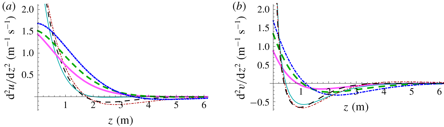
The most profound implications of the obtained solutions are concerned with the evolving current profiles caused by increasing wind: as in the case of periodic wind, the evolving profiles invariably exhibit inflection points and are likely to become strongly linearly unstable. The emergence of inflection points in the current profiles  $u(z,t)$ and
 $v(z,t)$ in all three models is illustrated in figure 6. Here, we do not quantify the growth rates of these instabilities, which for the reasons we have already discussed goes beyond the scope of this work. We reiterate, that often such instabilities have high growth rates and we can expect almost instant (compared to the inertial time scale) development of larger vortices (or rolls) in the already turbulent flow. Certainly, the Ekman model, which is based on the assumption of horizontal uniformity, is no longer applicable for such situations. Note the vertical localization of the expected turbulence spike: in our sample examples the layers of expected intense mixing occur near the surface, while most of the models predict enhanced mixing near the bottom of the mixed layer. To our knowledge, none of the existing much more sophisticated models of turbulent closures employed for modelling of the surface boundary-layer dynamics can capture such short-lived strongly localized events.
The curvatures of the velocity profiles  $u^{\prime \prime }(z,t)$ and
 $v^{\prime \prime }(z,t)$ as functions of depth in two models of viscosity: constant (thick lines) and time-dependent vertically uniform viscosity (thin lines). Three different moments are considered:
 $\tilde{t}=2$ (solid lines),
 $\tilde{t}=3$ (dashed lines) and
 $\tilde{t}=5$ (dotted lines). The parameters:
 $\unicode[STIX]{x1D6FF}=3~\text{h}$,
 $f=10^{-4}~\text{s}^{-1}$,
 $\unicode[STIX]{x1D708}_{0}=10^{-4}~\text{m}^{2}~\text{s}^{-1}$.

5 Transient Ekman currents in time-dependent viscosity model with $\unicode[STIX]{x1D708}_{e}(z,t)=\unicode[STIX]{x1D708}_{e}(t)\unicode[STIX]{x1D708}_{0}(1+z/\unicode[STIX]{x1D6FC}(t))^{\unicode[STIX]{x1D707}}$

Although the linear dependence of eddy viscosity with depth we adopted in the previous sections is supported by both naive translation of the wall layer ideology and large-eddy simulations by Zikanov et al. (Reference Zikanov, Slinn and Dhanak2003), the observations in the ocean often reveal a more complicated picture. There are a number of studies which report observations of a logarithmic layer near the surface as a universal phenomenon (e.g. Csanady Reference Csanady2001), while other authors report a more complicated picture (e.g. Kudryavtsev et al. Reference Kudryavtsev, Shrira, Dulov and Malinovsky2008) and some more complicated empirical parameterizations of  $\unicode[STIX]{x1D708}_{e}(z)$ were put forward (e.g. Large et al. Reference Large, McWilliams and Doney1994). It is not clear how well the aggregated data were controlled for the absence of solar heating and night convection, which violate our basic assumptions. In the oceanographic community there is a need for nonlinear with respect to depth parameterizations of
 $\unicode[STIX]{x1D708}_{e}(z)$. The implications of a nonlinear parameterization of eddy viscosity for Ekman currents are not clear; there is no applicable mathematical model. In § 3 we sketched the derivation of the general solution for a wide class of self-similar profiles,
 $$\begin{eqnarray}\displaystyle \unicode[STIX]{x1D708}_{e}(z,t)=\unicode[STIX]{x1D708}_{0}\unicode[STIX]{x1D708}_{e1}(t)\left[(1+z/\unicode[STIX]{x1D6FC}(t))^{\unicode[STIX]{x1D707}}\right],\quad (\unicode[STIX]{x1D707}>0), & & \displaystyle\end{eqnarray}$$
where  $\unicode[STIX]{x1D6FC}(t)$ is real and positive and
 $\unicode[STIX]{x1D708}_{0}$ is constant. For viscosity that is constant in time Jordan & Baker (Reference Jordan and Baker1980) derived solutions in terms of Bessel functions for the steady Ekman current, they also examined the non-steady problem but have not obtained a compact closed solution. Employing their results as a starting point in appendix A we obtain solutions (A 27) for the time- and depth-dependent profiles given by (5.1).
Leaving aside the question of whether the obtained solutions occur in reality, there is also a legitimate question: if transient Ekman currents do occur, how might a nonlinear depth dependence of viscosity affect their dynamics. To our knowledge, there have been no studies of this issue.
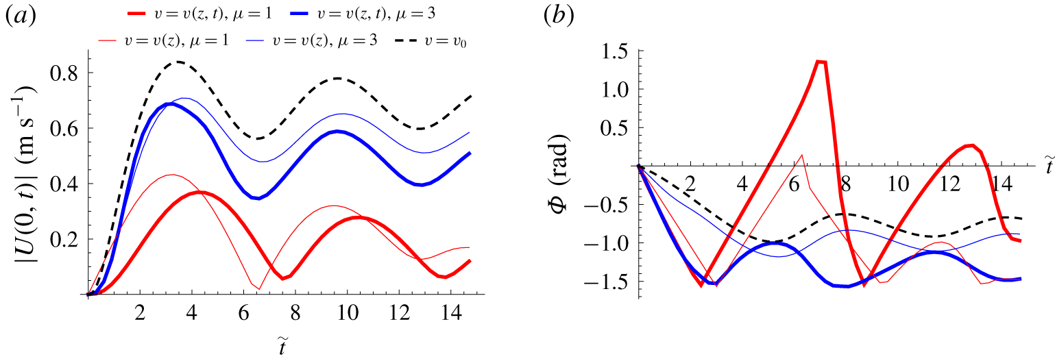
Evolution of Ekman currents from rest under growing wind (with the growth time scale  $\unicode[STIX]{x1D6FF}=2~\text{h}$) ending up with a plateau in five different models: two time–depth-dependent viscosity models with eddy viscosity
 $\unicode[STIX]{x1D708}_{e}(z,t)=\unicode[STIX]{x1D708}_{e1}(t)[\unicode[STIX]{x1D708}_{0}(1+z/\unicode[STIX]{x1D6FC})^{\unicode[STIX]{x1D707}}]$, where
 $\unicode[STIX]{x1D707}=1$ and
 $\unicode[STIX]{x1D707}=3$; two models with
 $\unicode[STIX]{x1D708}_{e1}(t)=\text{const.}$, the depth-only dependent viscosity models with
 $\unicode[STIX]{x1D707}=1,3$; the classical Ekman model with constant eddy viscosity
 $\unicode[STIX]{x1D708}=\unicode[STIX]{x1D708}_{0}$. Time is scaled as in all previous plots:
 $\tilde{t}=ft$. (a) Current speed at the surface
 $|\boldsymbol{U}(0,t)|$. (b) The deflection angle
 $\unicode[STIX]{x1D6F7}(t)$ (between the surface current and the wind). The parameter values are:
 $f=10^{-4}~\text{s}^{-1}$,
 $\unicode[STIX]{x1D708}_{0}\approx 0.000625~\text{m}^{2}~\text{s}^{-1}$,
 $H=400~\text{m}$,
 $\unicode[STIX]{x1D6FC}=50~\text{m}$,
 $\unicode[STIX]{x1D70C}=1027~\text{kg}~\text{m}^{-3}$,
 $\unicode[STIX]{x1D70F}_{0}=0.175~\text{N}~\text{m}^{-2}$,
 $|U_{10}|=10~\text{m}~\text{s}^{-1}$.

To illustrate the effect of an eddy viscosity nonlinear dependence on depth in the case of constant  $\unicode[STIX]{x1D6FC}$ we compare the evolution of the Ekman currents for an example where the motion starts from rest and is forced by the same gradually increasing wind, ending up with a plateau. Figure 7 shows the evolution of Ekman currents at the surface predicted by five different models of eddy viscosity: two time-and-depth-dependent viscosity models with linear (
 $\unicode[STIX]{x1D707}=1$) and nonlinear (
 $\unicode[STIX]{x1D707}=3$) depth dependence with
 $\unicode[STIX]{x1D6FC}$ constant, two models with a depth-only dependent viscosity with
 $\unicode[STIX]{x1D707}=1$ and
 $\unicode[STIX]{x1D707}=3$ and a constant eddy viscosity. While the constant and linear in depth viscosity models were considered for an infinitely deep ocean, in the models with
 $\unicode[STIX]{x1D707}=3$ the depth
 $H$ was taken to be large but finite. It has been checked that the chosen value
 $H=400~\text{m}$ is large enough for the results not to depend noticeably on it. The evolution of the magnitude of surface velocity proved to be qualitatively the same in all five models: an increase upon turn on of the wind up to a plateau with superimposed decaying near-inertial oscillations. The characteristics of the pattern which are the most sensitive to the model of viscosity are the rate of growth after the turn on of the wind and the height of the plateau. The growth rate and the height of the plateau are maximal for the constant viscosity model. The cubic viscosity models, i.e. with
 $\unicode[STIX]{x1D708}_{e}(z,t)=\unicode[STIX]{x1D708}_{e1}(t)[\unicode[STIX]{x1D708}_{0}(1+z/\unicode[STIX]{x1D6FC})^{3}]$, predict somewhat smaller, but close, values of the growth rate and the plateau height for both the time–depth-dependent and depth-only dependent cases. In the models with linear depth dependence, the time dependence noticeably slows down and, at the same time, prolongs the growth. The magnitude of the near-inertial oscillations (with respect to the plateau) is the smallest in the model with constant-in-time cubic viscosity, while the constant-in-time linear viscosity leads to the largest amplitude of the oscillations. This is consistent with our overall understanding of the picture: the viscosity time dependence acts as an effective increase in the wind time scale
 $\unicode[STIX]{x1D6FF}$ and hence leads to weaker inertial oscillations. However, in this context, as figure 7(a) clearly shows, the effect of viscosity time dependence, although not negligible, is much weaker than the effect of the depth dependence.
The behaviour of the deflection angle  $\unicode[STIX]{x1D6F7}$ in the four models, although qualitatively similar (the current first rotates to the right and after reaching the maximal deflection exhibits decaying oscillations around a certain deflection level), differs quantitatively quite substantially. The amplitude of these oscillations is the feature most sensitive to the viscosity dependence: the largest oscillations (up to
 $\pm \unicode[STIX]{x03C0}/2$) occur in the model with time-and-depth-dependent viscosity with
 $\unicode[STIX]{x1D707}=1$, while the model with constant viscosity predicts the smallest (
 ${\sim}\pm 0.1\unicode[STIX]{x03C0}$) oscillations. The models with time-dependent viscosity exhibit noticeably larger oscillations than their counterparts with viscosities that are constant in time. At the present we cannot explain all the intricacies of these differences. We do not know how representative the chosen values of the parameters are. What the figure makes clear is that the evolution of surface Ekman currents is very sensitive to the choice of the eddy viscosity parameterization. This is probably the only conclusion we could make now with confidence. The above discussion of a single model example, although obviously insufficient for general conclusions, suggests that, because of their sensitivity to the choice of eddy viscosity parameterization and insufficient constraint of this choice by the available data, the Ekman models in their present shape are unfit to describe quantitatively the dynamics of Ekman currents. To advance our understanding, a dedicated study examining the Ekman layer dynamics in a wider range of models and parameters is needed.
6 Stokes–Ekman layer in models with time- and depth-dependent eddy viscosity
The picture of the ocean Ekman current dynamics outlined above does not take into account the ubiquitous surface waves, despite the common knowledge that whenever there is wind, wind waves are nearly always present. The exceptions include the situations with the water surface covered by floating ice, i.e. similar to those encountered by Nansen (Reference Nansen1905) and theoretically investigated by Ekman (Reference Ekman1905). The account of surface waves can essentially affect the Ekman current dynamics compared to the classical Ekman model, as was first suggested by Huang (Reference Huang1979). The effect of the wave-induced Stokes drift on Ekman currents was examined in a substantial number of works (see e.g. Xu & Bowen Reference Xu and Bowen1994, McWilliams, Sullivan & Moeng Reference McWilliams, Sullivan and Moeng1997, Lewis & Belcher Reference Lewis and Belcher2004, Polton, Lewis & Belcher Reference Polton, Lewis and Belcher2005, Ardhuin et al. Reference Ardhuin, Marié, Rascle, Forget and Roland2009 and Sullivan & McWilliams Reference Sullivan and McWilliams2010), it has been confirmed that this effect can indeed be essential: the deflection of the current from the wind direction was found to be particularly strongly affected (McWilliams et al. Reference McWilliams, Sullivan and Moeng1997; Lewis & Belcher Reference Lewis and Belcher2004). However, in the literature, consideration was confined to somewhat oversimplified models. In particular, the eddy viscosity was assumed to be either constant (both in space and time) and isotropic, or isotropic, constant in time and linearly varying with depth (Lewis & Belcher Reference Lewis and Belcher2004), while the wave spectrum was, as a rule, modelled by a single harmonic; crucially, the Stokes drift dynamics caused by wave field evolution was ignored. It is indeed plausible to consider a quasi-stationary wave field subjected to a constant wind for a relatively short period. However, since the characteristic time scale of the Ekman currents subjected to variable winds is several inertial periods, for a quantitative study it is as questionable to assume constant eddy viscosity as to consider the Stokes drift to be constant in time. Note that, even under a constant wind the Stokes drift cannot remain constant, the dominant wavelength increases with time on a time scale which might be comparable to or smaller than the scale of Ekman layer formation. At present, there is no study of Ekman currents subjected to variable winds interacting with an evolving wave field. In this section we partly address this gap. We consider how a time-dependent Stokes drift with a more realistic vertical profile of time-dependent viscosity could be incorporated into the picture of Ekman current dynamics without these too restrictive assumptions.
Accounting for the Stokes drift, the ‘Stokes–Ekman’ equations take the form (e.g. Xu & Bowen Reference Xu and Bowen1994; Sullivan & McWilliams Reference Sullivan and McWilliams2010),
 $$\begin{eqnarray}\displaystyle \frac{\unicode[STIX]{x2202}\boldsymbol{U}}{\unicode[STIX]{x2202}t}+\text{i}f(\boldsymbol{U}+\boldsymbol{U}_{s})=\frac{\unicode[STIX]{x2202}}{\unicode[STIX]{x2202}z}\left(\unicode[STIX]{x1D708}_{e}(z,t)\frac{\unicode[STIX]{x2202}\boldsymbol{U}}{\unicode[STIX]{x2202}z}\right), & & \displaystyle\end{eqnarray}$$
where  $\boldsymbol{U}_{s}=U_{s}(z,t)\boldsymbol{e}_{U}$ is the Stokes drift due to surface waves as a function of time and depth,
 $\boldsymbol{e}_{U}$ is unit vector in the mean direction of wave propagation (not necessarily coinciding with the direction of wind), the rest of the notation remains the same as in the previous sections:
 $\boldsymbol{U}=U(z,t)+\text{i}V(z,t)$,
 $\unicode[STIX]{x1D708}_{e}=\unicode[STIX]{x1D708}_{e}(z,t)$. To leading order, the Stokes drift is provided by integration in the wavevector space over all wavevectors of the wave spectrum,
 $$\begin{eqnarray}\displaystyle \boldsymbol{U}_{s}(z,t)={\textstyle \frac{1}{2}}\int _{0}^{\unicode[STIX]{x1D714}_{c}}\int _{0}^{2\unicode[STIX]{x03C0}}\unicode[STIX]{x1D714}\boldsymbol{k}(\unicode[STIX]{x1D714},\unicode[STIX]{x1D703})E(\unicode[STIX]{x1D714},\unicode[STIX]{x1D703},t)\text{e}^{-2|\boldsymbol{k}|z}\,\text{d}\unicode[STIX]{x1D714}\,\text{d}\unicode[STIX]{x1D703}, & & \displaystyle\end{eqnarray}$$
where  $E(\unicode[STIX]{x1D714},\unicode[STIX]{x1D703},t)$ is the directional energy spectrum (presumed to be given in our context),
 $\unicode[STIX]{x1D714}$ is the frequency of a monochromatic wave component with a wavevector
 $\boldsymbol{k}$,
 $\unicode[STIX]{x1D714}_{c}$ is a cutoff frequency; the specific choice of the cutoff scale is of little significance. Strictly speaking, the
 $z$-dependence of each spectral component is not exponential, as is well known from available solutions of the boundary value problem for waves upon a sheared current (e.g. Kirby & Chen Reference Kirby and Chen1989). The, usually neglected in this context,
 $O(\boldsymbol{k}\boldsymbol{U}|_{(z=0)}/\unicode[STIX]{x1D714})$ correction depends on the profile and direction of the Ekman current. The neglect of the dependence of surface mode vertical structure on the boundary-layer profile decouples
 $\boldsymbol{U}_{s}$ from
 $\boldsymbol{U}(z,t)$ and dramatically simplifies the problem. Although here we follow the established practice and also neglect the effect of the Ekman current on the mode structure, we seem to be the first to note that in doing so we are neglecting a wave–current interaction mechanism which might prove important for wave modelling over large distances and, therefore, is worth investigating. Such a study, however, requires a dedicated work.
In contrast to the purely local ocean response in the classical Ekman model, the time dependence of the directional wave spectrum  $E(\unicode[STIX]{x1D714},\unicode[STIX]{x1D703},t)$, as a rule, is determined not by the local wind but by the history of wind over a large area (e.g. Komen, Cavaleri & Donelan Reference Komen, Cavaleri and Donelan1996). Here, assuming it to be known from a wave model, we just note that the characteristic time scale of
 $\boldsymbol{U}_{s}$ could be either comparable to characteristic time scales of wind variability or, as a rule, exceed them.
It is convenient to rewrite equation (6.1) as the standard Ekman equation with an added ‘forcing’ right-hand side due to the Stokes drift,
 $$\begin{eqnarray}\displaystyle \frac{\unicode[STIX]{x2202}\boldsymbol{U}}{\unicode[STIX]{x2202}t}+\text{i}f\boldsymbol{U}-\frac{\unicode[STIX]{x2202}}{\unicode[STIX]{x2202}z}\left(\unicode[STIX]{x1D708}_{e}(z,t)\frac{\unicode[STIX]{x2202}\boldsymbol{U}}{\unicode[STIX]{x2202}z}\right)=-\text{i}f\boldsymbol{U}_{s}(z,t). & & \displaystyle\end{eqnarray}$$
The term  $\text{i}fU_{s}$ is sometimes referred to as the ‘Coriolis–Stokes force’. The flow is subjected to the same boundary conditions given by (2.5), (2.6). The initial condition specifies the velocity field at the initial moment
 $t=0$:
 $\boldsymbol{U}(z,0)$.
The general solution of (6.3) for arbitrary  $\boldsymbol{U}_{s}(z,t)$ and
 $\boldsymbol{U}(z,0)$ satisfying the boundary conditions (2.5) and (2.6) is derived in appendix B. The solution given by (B 9), (B 10) and (B 12) is expressed in terms of integrals of the modified Bessel functions
 $\text{I}_{0}$ and
 $\text{K}_{0}$. The formulae provide complete analytical solution describing transient Ekman currents caused by an arbitrarily changing wind under the assumption of a time-dependent eddy viscosity linearly increasing with depth.
To apply the obtained formulae, the time dependence of the Stokes drift has to be prescribed. To this end, one has to know the history of the evolution of the wave spectra over a considerable area. For example, if we are interested in describing the Ekman current dynamics on time scales of 10 hours or 10 days, we would need to model the evolution of wave spectra over fetches of approximately  $4\times 10^{2}$ or
 $10^{4}$ km and to know the wave spectra history over 10 hours or 10 days respectively. Since wave modelling on such a scale is routinely carried out by global and regional wave models, it is tempting to add an Ekman current block to the existing wave models. Wave spectrum evolution is, in turn, affected by Ekman currents. To our knowledge the feedback effect of Ekman currents on the wave field evolution has never been discussed and quantified in the literature; it might be noticeable for large fetches. Now we have got at our disposal a new tool which, by providing a better description of these currents, might help in improving wave modelling. Although the use of a ‘WAM’ or ‘Wavewatch’-type wave model (e.g. www.bodc.ac.uk/data/documents/nodb/254628/, https://polar.ncep.noaa.gov/waves/wavewatch/) with an Ekman current block looks straightforward, it goes beyond the scope of the present work and requires a dedicated study. Here, in the spirit of this work, which is an entirely analytical study, we confine ourselves to a single qualitative conclusion which, to our knowledge, has not been mentioned in the literature: accounting for the Stokes drift makes the existence of the steady Ekman current impossible since, even under a steady wind, the wave field always continues to evolve. The question on how the Ekman layer evolves due to nonlinear evolution of the wave field will be elaborated elsewhere.
7 Concluding remarks
Our main conclusions could be summarized as follows. We showed that the Ekman theory could be extended to take into account time- and depth-dependent eddy viscosity, which is expected to be a better reflection of reality. Under the assumption of self-similar time- and depth-dependent eddy viscosity, which includes as a subclass the situations with arbitrary power-law depth dependence of eddy viscosity and arbitrary time dependence of the wind, we found exact general solution to the Ekman equations with time- and depth-dependent viscosity. This general solution describes the dynamics of the Ekman boundary layer in terms of an explicit Green’s function expressed via modified Bessel functions. This novel broad class of exact solutions to the Navier–Stokes equations is of interest per se.
From the viewpoint of possible applications, our examination of the basic scenarios demonstrates that taking into account both the depth and time dependences of the eddy viscosity substantially affect the Ekman current response. We did not attempt to explore the parameter space and, hence, do not know how representative the examples of evolution we investigated are. For the fundamental reasons we discuss below, we are reluctant to draw any specific conclusions on the effect of accounting for the time and depth dependence of the eddy viscosity.
The solutions describing transient Ekman currents in models with time- and depth-dependent eddy viscosity were further extended by taking into account the time- and depth-dependent Stokes drift created by evolving wave spectra. The general solution of the corresponding Stokes–Ekman equations has been derived to fill the gap in the existing literature. Possibilities for the coupling of existing wave models with the Stokes–Ekman equations and as yet unaccounted for mechanisms of coupling were also discussed.
In nature, the eddy viscosity (recall that it is merely a parametrization) does depend on time, although the dependence might be more complicated than the scaling in terms of the  $u_{\ast }$ we adopted. There is a potential to extend our approach by considering non-local in time relations between wind and eddy viscosity, which we did not explore here. A natural first step in this direction would be to consider a time-dependent eddy viscosity with a time delay, which we have not attempted here.
In this work we did not attempt a comparison with data. The fact that our solutions for time-dependent linear-in-depth viscosity predict noticeably smaller surface current deflection to the wind direction, which better agrees with the observations, is not sufficient to be treated as a vindication of our approach. The data are too scattered and each case has to be thoroughly studied before any far reaching conclusions are made. A salient feature of the Ekman currents forced by the varying wind is that the obtained transient solutions do not resemble the steady solutions, for example, they do not develop the Ekman spirals, even if the wind is varying slowly.
Probably our most significant finding is that of the intrinsic contradictions of the Ekman-type models and all their generalizations used for modelling of the oceanic surface boundary layer. To our knowledge, these contradictions, which we briefly discuss below, have not been mentioned in the literature. Subjected to a growing or turning wind, the Ekman current response develops profiles which are likely to become unstable. We found that these instabilities are of small scale (with wavelengths  ${\sim}10^{2}~\text{m}$) but with wavelengths far exceeding the characteristic thickness of the Ekman currents (this separation of scales enables one to find the characteristics of the instabilities asymptotically). They proved to be very sensitive to the adopted model of eddy viscosity. Crucially, the instabilities are fast compared to the inertial time scale and, thus, to the characteristic time scales of the Ekman current dynamics. This raises questions about the fundamentals of the Ekman type models. Only during its stable initial phase could the Ekman current evolution from rest be faithfully captured within the framework of the Ekman paradigm. When strong instabilities occur, we could expect a substantial deviation from the obtained Ekman solutions; horizontally and vertically localized dramatically enhanced ‘spike’ mixing (compared to the models assuming merely diffusion of momentum) in the corresponding parts of the water column is the most likely outcome. Thus, we could expect two-scale mixing characterized by widely separated temporal scales: ‘normal’ diffusion of momentum and a ‘spike mixing’ caused by the inflectional instabilities. The fast evolving part of the current profile is expected to reach a stable configuration at the time scale of instability, then only the slow evolution of the current will continue, until the varying wind creates another instance of a strongly unstable inflectional profile. An immediate implication of this new qualitative picture is that a gusty wind should produce a broader boundary layer than a smooth wind of comparable strength. The occurrence of such strong instabilities of transient Ekman currents undermines the very existence of the Ekman paradigm. The instabilities violate the basic assumption of the presumed horizontal uniformity of the flow. In principle, it might still be possible to preserve Ekman models by interpreting them in a coarse grain sense (averaging over certain time and spatial scales and using a bulk viscosity). For example, the presence of Langmuir circulations, which breaks down the key assumption of horizontal isotropy of the eddy viscosity, is dealt with by considering non-diagonal tensor of Reynolds stresses (Wirth Reference Wirth2010). However, at present it is not clear how to apply such an averaging and how the scale of averaging is linked to the parameters of Langmuir circulations. This example is aimed just to highlight a general lack of clarity regarding the scales of spatial and temporal averaging implicit in the Ekman type models. We conclude that, at present, the Ekman models cannot be seriously considered as rational models (after the occurrence of instability), since we do not know when/whether they work and with what accuracy. Hence, to preserve the established Ekman paradigm, it needs a radical revision.
Although the prime motivation for this work came from the oceanic surface boundary-layer context, the implications of the findings are not confined to the upper ocean. The Ekman layers are ubiquitous and our findings, and especially the general questions we raised, might be relevant in many other contexts as well. The present work has just highlighted the problem, the issue certainly needs further study and will be explored elsewhere.
Acknowledgements
The authors thank R. Danyi for his help in examining the instabilities, M. Luneva for helpful discussions and an anonymous referee for very helpful comments. The hospitality of the University of Toulon, where this work was revised by V.I.S., and stimulating discussions with P. Fraunié are greatly appreciated. The work was partly supported by UK NERC grant NE/M016269/1, by EU grant FP7 612610 and by Libyan Ministry of Education grant 469, which is gratefully acknowledged.
Declaration of interests
The authors report no conflict of interest.
Appendix A. Time-dependent viscosity model with $\unicode[STIX]{x1D708}_{e}(z,t)=\unicode[STIX]{x1D708}_{e}(t)\unicode[STIX]{x1D708}_{0}(1+z/\unicode[STIX]{x1D6FC}(t))^{\unicode[STIX]{x1D707}}$

Here, we provide the derivation of the general solution for the following class of self-similar profiles,
 $$\begin{eqnarray}\displaystyle \unicode[STIX]{x1D708}_{e}(z,t)=\unicode[STIX]{x1D708}_{0}\unicode[STIX]{x1D708}_{e1}(t)\left[(1+z/\unicode[STIX]{x1D6FC}(t))^{\unicode[STIX]{x1D707}}\right],\quad (\unicode[STIX]{x1D707}>0), & & \displaystyle\end{eqnarray}$$
where  $\unicode[STIX]{x1D6FC}(t)$ is real and positive and
 $\unicode[STIX]{x1D708}_{0}$ is constant.
Consider the standard Ekman equations
 $$\begin{eqnarray}\displaystyle & \displaystyle \frac{\unicode[STIX]{x2202}\boldsymbol{U}}{\unicode[STIX]{x2202}t}+\text{i}f\boldsymbol{U}=\frac{\unicode[STIX]{x2202}}{\unicode[STIX]{x2202}z}\left(\unicode[STIX]{x1D708}_{e}(z,t)\frac{\unicode[STIX]{x2202}\boldsymbol{U}}{\unicode[STIX]{x2202}z}\right), & \displaystyle\end{eqnarray}$$
 $$\begin{eqnarray}\displaystyle & \displaystyle \frac{\unicode[STIX]{x2202}\boldsymbol{U}}{\unicode[STIX]{x2202}z}=\frac{-\unicode[STIX]{x1D749}(t)}{\unicode[STIX]{x1D70C}\unicode[STIX]{x1D708}_{e}(z,t)}\quad \text{at }z=0, & \displaystyle\end{eqnarray}$$
 $$\begin{eqnarray}\displaystyle & \displaystyle \boldsymbol{U}=0\quad \text{as }z\rightarrow \infty , & \displaystyle\end{eqnarray}$$
for a class of self-similar eddy viscosity distributions (A 1). The substitution,
 $$\begin{eqnarray}\displaystyle \boldsymbol{U}(z,t)=\text{e}^{-\text{i}ft}\boldsymbol{W}(z,T),\quad T=\unicode[STIX]{x1D708}_{0}\int _{0}^{t}\unicode[STIX]{x1D708}_{e1}(\unicode[STIX]{x1D709})\,\text{d}\unicode[STIX]{x1D709}, & & \displaystyle\end{eqnarray}$$
turns the Ekman system (A 2) into a more tractable one,
 $$\begin{eqnarray}\displaystyle \displaystyle \frac{\unicode[STIX]{x2202}\boldsymbol{W}}{\unicode[STIX]{x2202}T}=\frac{\unicode[STIX]{x2202}}{\unicode[STIX]{x2202}z}\left[\left(1+\frac{z}{\unicode[STIX]{x1D6FC}(t)}\right)^{\unicode[STIX]{x1D707}}\frac{\unicode[STIX]{x2202}\boldsymbol{W}}{\unicode[STIX]{x2202}z}\right], & & \displaystyle\end{eqnarray}$$
 $$\begin{eqnarray}\displaystyle \displaystyle \frac{\unicode[STIX]{x2202}\boldsymbol{W}}{\unicode[STIX]{x2202}z}=\frac{-\text{e}^{\text{i}ft(T)}\unicode[STIX]{x1D749}(t(T))}{\unicode[STIX]{x1D70C}\unicode[STIX]{x1D708}_{e}(z,t(T))}\quad \text{at }z=0, & & \displaystyle\end{eqnarray}$$
 $$\begin{eqnarray}\displaystyle \displaystyle \boldsymbol{W}=0\quad \text{as }z\rightarrow \infty . & & \displaystyle\end{eqnarray}$$
Introducing new independent variables,
 $$\begin{eqnarray}Z=1+\frac{z}{\unicode[STIX]{x1D6FC}(t(T))};\quad T_{1}=\int _{0}^{T}\frac{1}{\unicode[STIX]{x1D6FC}^{2}(t(\unicode[STIX]{x1D701}))}\,\text{d}\unicode[STIX]{x1D701},\end{eqnarray}$$
and noting that,
 $$\begin{eqnarray}\frac{\unicode[STIX]{x2202}\boldsymbol{W}}{\unicode[STIX]{x2202}z}=\frac{1}{\unicode[STIX]{x1D6FC}(t(T))}\frac{\unicode[STIX]{x2202}\boldsymbol{W}}{\unicode[STIX]{x2202}Z},\quad \frac{\unicode[STIX]{x2202}^{2}\boldsymbol{W}}{\unicode[STIX]{x2202}z^{2}}=\frac{1}{\unicode[STIX]{x1D6FC}^{2}(t(T))}\frac{\unicode[STIX]{x2202}^{2}\boldsymbol{W}}{\unicode[STIX]{x2202}Z^{2}},\end{eqnarray}$$
enables us to simplify the system (A 6)–(A 8) into,
 $$\begin{eqnarray}\displaystyle & \displaystyle \frac{\unicode[STIX]{x2202}\boldsymbol{W}}{\unicode[STIX]{x2202}T_{1}}=\frac{\unicode[STIX]{x2202}}{\unicode[STIX]{x2202}Z}\left[Z^{\unicode[STIX]{x1D707}}\frac{\unicode[STIX]{x2202}\boldsymbol{W}}{\unicode[STIX]{x2202}Z}\right], & \displaystyle\end{eqnarray}$$
 $$\begin{eqnarray}\displaystyle & & \displaystyle \nonumber\\ \displaystyle & \displaystyle \frac{\unicode[STIX]{x2202}\boldsymbol{W}}{\unicode[STIX]{x2202}Z}=\frac{-\text{e}^{\text{i}ft(T_{1})}\unicode[STIX]{x1D6FC}(t(T_{1}))\unicode[STIX]{x1D749}(t(T_{1}))}{\unicode[STIX]{x1D70C}\unicode[STIX]{x1D708}_{0}\unicode[STIX]{x1D708}_{e1}(t(T_{1}))Z^{\unicode[STIX]{x1D707}}}=\boldsymbol{G}(T_{1})\quad \text{at }Z=1, & \displaystyle\end{eqnarray}$$
 $$\begin{eqnarray}\displaystyle & & \displaystyle \nonumber\\ \displaystyle & \displaystyle \boldsymbol{W}=0\quad \text{as }Z\rightarrow \infty . & \displaystyle\end{eqnarray}$$
By taking the Laplace transform of (A 9) with respect to  $T_{1}$ (
 ${\mathcal{L}}\{\boldsymbol{W}(T_{1})\}=\hat{\boldsymbol{W}}(s)$) we find,
 $$\begin{eqnarray}\displaystyle Z^{\unicode[STIX]{x1D707}}\frac{\text{d}^{2}\hat{\boldsymbol{W}}}{\text{d}Z^{2}}+\unicode[STIX]{x1D707}Z^{\unicode[STIX]{x1D707}-1}\frac{\text{d}\hat{\boldsymbol{W}}}{\text{d}Z}-s\hat{\boldsymbol{W}}=0. & & \displaystyle\end{eqnarray}$$
One more change of variables,
 $$\begin{eqnarray}\displaystyle \hat{\boldsymbol{W}}=S_{1}^{\unicode[STIX]{x1D70E}}\unicode[STIX]{x1D6F9}(S_{1});\quad S_{1}=\frac{1}{|1-\unicode[STIX]{x1D707}/2|}Z^{1-\unicode[STIX]{x1D707}/2};\quad \unicode[STIX]{x1D70E}=\frac{1}{2}\left(\frac{1-\unicode[STIX]{x1D707}}{1-\unicode[STIX]{x1D707}/2}\right) & & \displaystyle\end{eqnarray}$$
yields,
 $$\begin{eqnarray}\displaystyle \frac{\text{d}\hat{\boldsymbol{W}}}{\text{d}Z}=S_{1}^{\unicode[STIX]{x1D70E}}\frac{\text{d}\unicode[STIX]{x1D6F9}}{\text{d}S_{1}}\frac{\text{d}S_{1}}{\text{d}Z}+\unicode[STIX]{x1D70E}S_{1}^{\unicode[STIX]{x1D70E}-1}\frac{\text{d}S_{1}}{\text{d}Z}\unicode[STIX]{x1D6F9}(S_{1}), & & \displaystyle\end{eqnarray}$$
and,
 $$\begin{eqnarray}\displaystyle \frac{\text{d}^{2}\tilde{\boldsymbol{W}}}{\text{d}Z^{2}} & = & \displaystyle S_{1}^{\unicode[STIX]{x1D70E}}\left(\frac{\text{d}S_{1}}{\text{d}Z}\right)^{2}\frac{\text{d}^{2}\unicode[STIX]{x1D6F9}}{\text{d}S_{1}^{2}}+\left[S_{1}^{\unicode[STIX]{x1D70E}}\frac{\text{d}^{2}S_{1}}{\text{d}Z^{2}}+2\unicode[STIX]{x1D70E}S_{1}^{\unicode[STIX]{x1D70E}-1}\left(\frac{\text{d}S_{1}}{\text{d}Z}\right)^{2}\right]\frac{\text{d}\unicode[STIX]{x1D6F9}}{\text{d}S_{1}}\nonumber\\ \displaystyle & & \displaystyle +\,\left[\unicode[STIX]{x1D70E}S_{1}^{\unicode[STIX]{x1D70E}-1}\frac{\text{d}^{2}S_{1}}{\text{d}Z^{2}}+\unicode[STIX]{x1D70E}(\unicode[STIX]{x1D70E}-1)S_{1}^{\unicode[STIX]{x1D70E}-2}\left(\frac{\text{d}S_{1}}{\text{d}Z}\right)^{2}\right]\unicode[STIX]{x1D6F9}(S_{1}).\end{eqnarray}$$
On substituting (A 13), (A 14) and (A 15) into equation (A 12), we obtain,
 $$\begin{eqnarray}\displaystyle \frac{\text{d}^{2}\unicode[STIX]{x1D6F9}}{\text{d}S_{1}^{2}}+S_{1}^{-1}\frac{\text{d}\unicode[STIX]{x1D6F9}}{\text{d}S_{1}}-\left(\left(\frac{\unicode[STIX]{x1D707}-1}{2-\unicode[STIX]{x1D707}}\right)^{2}S_{1}^{-2}+s\right)\unicode[STIX]{x1D6F9}(S_{1})=0. & & \displaystyle\end{eqnarray}$$
Yet another change of independent variable,
 $$\begin{eqnarray}\displaystyle \unicode[STIX]{x1D701}=\text{i}S_{1}\sqrt{s} & & \displaystyle\end{eqnarray}$$
turns equation (A 16) into the Bessel equation,
 $$\begin{eqnarray}\displaystyle \unicode[STIX]{x1D701}^{2}\frac{\text{d}^{2}\unicode[STIX]{x1D6F9}}{\text{d}\unicode[STIX]{x1D701}^{2}}+\unicode[STIX]{x1D701}\frac{\text{d}\unicode[STIX]{x1D6F9}}{\text{d}\unicode[STIX]{x1D701}}+\left(\unicode[STIX]{x1D701}^{2}-\left(\frac{\unicode[STIX]{x1D707}-1}{2-\unicode[STIX]{x1D707}}\right)^{2}\right)\unicode[STIX]{x1D6F9}(\unicode[STIX]{x1D701})=0. & & \displaystyle\end{eqnarray}$$
Its general solution in terms of Bessel functions is (e.g. Abramowitz & Stegun Reference Abramowitz and Stegun1972),
 $$\begin{eqnarray}\displaystyle \unicode[STIX]{x1D6F9}=c_{1}J_{\unicode[STIX]{x1D70E}_{1}}(\unicode[STIX]{x1D701})+c_{2}Y_{\unicode[STIX]{x1D70E}_{1}}(\unicode[STIX]{x1D701});\quad \unicode[STIX]{x1D701}=\text{i}S_{1}\sqrt{s};\quad \unicode[STIX]{x1D70E}_{1}=\left|\frac{1-\unicode[STIX]{x1D707}}{-2+\unicode[STIX]{x1D707}}\right|. & & \displaystyle\end{eqnarray}$$
Then, the general solution of (A 12) can be written as,
 $$\begin{eqnarray}\displaystyle \hat{\boldsymbol{W}}(Z,s) & = & \displaystyle S_{1}^{\unicode[STIX]{x1D70E}}\unicode[STIX]{x1D6F9}(S_{1})\nonumber\\ \displaystyle & = & \displaystyle S_{1}^{\unicode[STIX]{x1D70E}}\left(c_{1}J_{\unicode[STIX]{x1D70E}_{1}}(iS_{1}\sqrt{s})+c_{2}Y_{\unicode[STIX]{x1D70E}_{1}}(iS_{1}\sqrt{s})\right)\nonumber\\ \displaystyle & = & \displaystyle S_{1}^{\unicode[STIX]{x1D70E}}\left(c_{1}i^{\unicode[STIX]{x1D70E}_{1}}I_{\unicode[STIX]{x1D70E}_{1}}(S_{1}\sqrt{s})+c_{2}Y_{\unicode[STIX]{x1D70E}_{1}}(\text{i}S_{1}\sqrt{s})\right),\end{eqnarray}$$
where
 $$\begin{eqnarray}I_{v}(x)=i^{-v}J_{v}(ix),\quad S_{1}=\frac{1}{|1-\unicode[STIX]{x1D707}/2|}Z^{1-\unicode[STIX]{x1D707}/2},\quad \unicode[STIX]{x1D70E}=\frac{1}{2}\left(\frac{1-\unicode[STIX]{x1D707}}{1-\unicode[STIX]{x1D707}/2}\right),\quad \unicode[STIX]{x1D70E}_{1}=\left|\unicode[STIX]{x1D70E}\right|.\end{eqnarray}$$
The boundary condition at infinity implies  $c_{1}=0$, hence,
 $$\begin{eqnarray}\hat{\boldsymbol{W}}(Z,s)=c_{2}S_{1}^{\unicode[STIX]{x1D70E}}Y_{\unicode[STIX]{x1D70E}_{1}}(iS_{1}\sqrt{s}).\end{eqnarray}$$
Making use of the Laplace form of the surface boundary condition (A 10),
 $$\begin{eqnarray}\frac{\text{d}\hat{\boldsymbol{W}}}{\text{d}Z}={\mathcal{L}}\{\boldsymbol{G}(T_{1})\}\quad \text{at }Z=1,\end{eqnarray}$$
provides us with  $c_{2}$,
 $$\begin{eqnarray}\displaystyle c_{2}=\frac{{\mathcal{L}}\{\boldsymbol{G}(T_{1})\}}{A}, & & \displaystyle\end{eqnarray}$$
where
 $$\begin{eqnarray}\displaystyle A & = & \displaystyle \frac{1-\unicode[STIX]{x1D707}}{2|1-\unicode[STIX]{x1D707}/2|^{\unicode[STIX]{x1D70E}}}Y_{\unicode[STIX]{x1D70E}_{1}}\left(\frac{\text{i}\sqrt{s}}{|1-\unicode[STIX]{x1D707}/2|}\right)-\frac{\text{i}(2+\unicode[STIX]{x1D707})\sqrt{s}}{|1-\unicode[STIX]{x1D707}/2|^{\unicode[STIX]{x1D70E}+1}}\nonumber\\ \displaystyle & & \displaystyle \times \,\left(Y_{\unicode[STIX]{x1D70E}_{1}-1}\left(\frac{\text{i}\sqrt{s}}{|1-\unicode[STIX]{x1D707}/2|}\right)-Y_{\unicode[STIX]{x1D70E}_{1}+1}\left(\frac{\text{i}\sqrt{s}}{|1-\unicode[STIX]{x1D707}/2|}\right)\right).\end{eqnarray}$$
Thus, the general solution of the system (A 9)–(A 11) in terms of  $Z$ and
 $T_{1}$ is
 $$\begin{eqnarray}\displaystyle \boldsymbol{W}(Z,T_{1})=\frac{1}{2\unicode[STIX]{x03C0}\text{i}}\int _{c-\text{i}\infty }^{c+\text{i}\infty }\text{e}^{sT_{1}}\hat{\boldsymbol{W}}(Z,s)\,\text{d}s;\quad c\geqslant 0, & & \displaystyle\end{eqnarray}$$
where,
 $$\begin{eqnarray}\displaystyle \tilde{\boldsymbol{W}}(Z,s)=c_{2}S_{1}^{\unicode[STIX]{x1D70E}}Y_{\unicode[STIX]{x1D70E}_{1}}(\text{i}S_{1}\sqrt{s}),\quad S_{1}=\frac{1}{|1-\unicode[STIX]{x1D707}/2|}Z^{1-\unicode[STIX]{x1D707}/2}, & & \displaystyle\end{eqnarray}$$
and  $c_{2}$ is given by (A 23) and (A 24). Finally, we can return to the original variables
 $z,t,U$,
 $$\begin{eqnarray}\displaystyle & \displaystyle z=\unicode[STIX]{x1D6FC}(t)(Z-1),\quad T_{1}=\int _{0}^{T}\frac{1}{\unicode[STIX]{x1D6FC}^{2}(t(\unicode[STIX]{x1D701}))}\,\text{d}\unicode[STIX]{x1D701}, & \displaystyle\end{eqnarray}$$
 $$\begin{eqnarray}\displaystyle & \displaystyle T=\unicode[STIX]{x1D708}_{0}\int _{0}^{t}\unicode[STIX]{x1D708}_{e1}(\unicode[STIX]{x1D709})\,\text{d}\unicode[STIX]{x1D709},\quad \boldsymbol{U}(z,t)=\text{e}^{-\text{i}ft}\boldsymbol{W}(z,T). & \displaystyle\end{eqnarray}$$
This is the most general solution to the Ekman current initial-value problem obtained so far. For constant  $\unicode[STIX]{x1D6FC}$ it is straightforward to extend it for a fluid of finite depth. However, the solution becomes more complicated (
 $c_{1}$ is no longer zero but a lengthy expression) and in view of the revealed intrinsic contradictions of the Ekman paradigm discussed in § 7, we feel little incentive to provide more complicated formulae or elaborate dynamics of the Ekman currents described by the solution (A 22)–(A 28), at least until these fundamental contradictions are somehow resolved.
Appendix B. Ekman response to varying wind within the Stokes–Ekman model with time-and-depth-dependent eddy viscosity. The derivation
Our starting point is the Stokes–Ekman equations satisfying the standard boundary conditions ((2.5), (2.6)),
 $$\begin{eqnarray}\displaystyle \frac{\unicode[STIX]{x2202}\boldsymbol{U}}{\unicode[STIX]{x2202}t}+\text{i}f(\boldsymbol{U}+\boldsymbol{U}_{s})=\frac{\unicode[STIX]{x2202}}{\unicode[STIX]{x2202}z}\left(\unicode[STIX]{x1D708}_{e}(z,t)\frac{\unicode[STIX]{x2202}\boldsymbol{U}}{\unicode[STIX]{x2202}z}\right), & & \displaystyle\end{eqnarray}$$
where  $\boldsymbol{U}_{s}=U_{s}(z,t)\boldsymbol{e}_{U}$ is the Stokes drift due to surface waves as a function of time and depth is given by (5.2),
 $\boldsymbol{e}_{U}$ is unit vector in the mean direction of wave propagation, the rest of the notations we retain from the previous sections:
 $\boldsymbol{U}=U(z,t)+\text{i}V(z,t)$,
 $\unicode[STIX]{x1D708}_{e}=\unicode[STIX]{x1D708}_{e}(z,t)$. Here we presume
 $U_{s}(z,t)$ and
 $\unicode[STIX]{x1D708}_{e}(z,t)$ to be given. Here, in contrast to § 3.1, instead of continuing our consideration of self-similar distributions of eddy viscosity (A 1), we confine our analysis to simpler separable eddy viscosity distributions:
 $\unicode[STIX]{x1D708}_{e}(z,t)=\unicode[STIX]{x1D708}_{e1}(t)g(z)$ and later on consider the simplest case only. Using the substitution
 $$\begin{eqnarray}\displaystyle \boldsymbol{U}(z,t)=\text{e}^{-\text{i}ft}\boldsymbol{W}(z,T);\quad \left(T=\int _{0}^{t}\unicode[STIX]{x1D708}_{e1}(\unicode[STIX]{x1D709})\,\text{d}\unicode[STIX]{x1D709}\right), & & \displaystyle\end{eqnarray}$$
we rewrite the Ekman equation (6.3) as an inhomogeneous equation with a time- and depth-dependent right-hand side which we denote as  $\boldsymbol{F}_{1}(z,t)$,
 $$\begin{eqnarray}\displaystyle \frac{\unicode[STIX]{x2202}\boldsymbol{W}}{\unicode[STIX]{x2202}T}-\frac{\unicode[STIX]{x2202}}{\unicode[STIX]{x2202}z}\left(g(z)\frac{\unicode[STIX]{x2202}\boldsymbol{W}}{\unicode[STIX]{x2202}z}\right)=\frac{-\text{i}f\text{e}^{\text{i}ft(T)}\boldsymbol{U}_{s}(z,t(T))}{\unicode[STIX]{x1D708}_{e1}(t(T))}\equiv \boldsymbol{F}_{1}(z,T). & & \displaystyle\end{eqnarray}$$
Taking the Laplace transform with respect to  $T$ (
 ${\mathcal{L}}\{\boldsymbol{W}(T)\}=\hat{\boldsymbol{W}}(s)$) yields,
 $$\begin{eqnarray}\displaystyle \frac{\text{d}}{\text{d}z}\left(g(z)\frac{\text{d}\hat{\boldsymbol{W}}}{\text{d}z}\right)-s\hat{\boldsymbol{W}}=-\hat{\boldsymbol{F}}_{1}(z,s)-\boldsymbol{W}(z,0)\equiv -\hat{\boldsymbol{F}}_{2}(z,s), & & \displaystyle\end{eqnarray}$$
where  $\boldsymbol{W}(z,0)$ is the velocity profile at the initial moment which we presume to be given. Thus arbitrary non-zero initial conditions are incorporated into the right-hand side. Now, for simplicity and by virtue of arguments of § 3, we confine ourselves to linear
 $g(z)$:
 $g(z)=g_{1}(z+z_{0})$. More general separable and self-similar profiles (A 1) could be handled similarly.
The general solution is a sum of the general solution of the homogeneous equation  $\hat{\boldsymbol{W}}_{h}(z,s)$ derived in § 3.1 and a particular solution
 $\hat{\boldsymbol{W}}_{p}(z,s)$ of equation (B 4), thus,
 $$\begin{eqnarray}\displaystyle \hat{\boldsymbol{W}}(z,s)=\hat{\boldsymbol{W}}_{h}(z,s)+\hat{\boldsymbol{W}}_{p}(z,s). & & \displaystyle\end{eqnarray}$$
Since the fundamental solutions of the homogeneous equation are known, it is straightforward to find a particular solution of the inhomogeneous equation,
 $$\begin{eqnarray}\displaystyle \frac{\text{d}^{2}\hat{\boldsymbol{W}}}{\text{d}z^{2}}+\frac{1}{z+z_{0}}\frac{\text{d}\hat{\boldsymbol{W}}}{\text{d}z}-\frac{s}{g_{1}(z+z_{0})}\hat{\boldsymbol{W}}=\frac{-\hat{\boldsymbol{F}}_{2}(z,s)}{g_{1}(z+z_{0})}. & & \displaystyle\end{eqnarray}$$
A particular solution of this equation can be expressed in terms of modified Bessel functions  $\text{I}_{0}$ and
 $\text{K}_{0}$,
 $$\begin{eqnarray}\displaystyle \hat{\boldsymbol{W}}_{p} & = & \displaystyle \frac{2}{g_{1}}\int _{0}^{z}\hat{\boldsymbol{F}}_{2}(\unicode[STIX]{x1D702},s)\left(-\text{I}_{0}\left[2\sqrt{\frac{(z+z_{0})s}{g_{1}}}\right]\text{K}_{0}\left[2\sqrt{\frac{(\unicode[STIX]{x1D702}+z_{0})s}{g_{1}}}\right]\right.\nonumber\\ \displaystyle & & \displaystyle \left.+\,\text{K}_{0}\left[2\sqrt{\frac{(z+z_{0})s}{g_{1}}}\right]\text{I}_{0}\left[2\sqrt{\frac{(\unicode[STIX]{x1D702}+z_{0})s}{g_{1}}}\right]\right)\text{d}\unicode[STIX]{x1D702}.\end{eqnarray}$$
Then, the general solution satisfying the boundary condition at infinity ( $\tilde{\boldsymbol{W}}\rightarrow 0$ as
 $z\rightarrow \infty$) becomes,
 $$\begin{eqnarray}\displaystyle \hat{\boldsymbol{W}}(z,s)=\text{K}_{0}\left[2\sqrt{\frac{(z+z_{0})s}{g_{1}}}\right]\left(c_{2}+(2/g_{1})\int _{0}^{z}\hat{\boldsymbol{F}}_{2}(\unicode[STIX]{x1D702},s)\text{I}_{0}\left[2\sqrt{\frac{(\unicode[STIX]{x1D702}+z_{0})s}{g_{1}}}\right]\text{d}\unicode[STIX]{x1D702}\right). & & \displaystyle\end{eqnarray}$$
The arbitrary constant  $c_{2}$ is specified by the boundary condition at the surface. To this end, the first derivative of the obtained general solution at
 $z=0$
 $$\begin{eqnarray}\displaystyle \frac{\text{d}\hat{\boldsymbol{W}}}{\text{d}z} & = & \displaystyle \frac{2}{g_{1}}\text{I}_{0}\left[2\sqrt{\frac{(z+z_{0})s}{g_{1}}}\right]\text{K}_{0}\left[2\sqrt{\frac{(z+z_{0})s}{g_{1}}}\right]\hat{\boldsymbol{F}}_{2}(z,s)-\nonumber\\ \displaystyle & & \displaystyle \frac{\sqrt{s}}{\sqrt{g_{1}(z+z_{0})}}K_{1}\left[2\sqrt{\frac{(z+z_{0})s}{g_{1}}}\right]\!\left(c_{2}+(2/g_{1})\int _{0}^{z}\hat{\boldsymbol{F}}_{1}(\unicode[STIX]{x1D702},s)\text{I}_{0}\left[2\sqrt{\frac{(\unicode[STIX]{x1D702}+z_{0})s}{g_{1}}}\right]\text{d}\unicode[STIX]{x1D702}\right)\nonumber\\ \displaystyle & & \displaystyle\end{eqnarray}$$
is substituted into the boundary condition at the surface ( $\hat{\boldsymbol{W}^{\prime }}(0,s)=\hat{\boldsymbol{F}}(s),\hat{\boldsymbol{F}}(s)={\mathcal{L}}[\boldsymbol{F}(T)]$), which yields the needed closed expression for
 $c_{2}$,
 $$\begin{eqnarray}\displaystyle c_{2}=\frac{\sqrt{g_{1}z_{0}}}{\sqrt{s}K_{1}\left[2\sqrt{\displaystyle \frac{sz_{0}}{g_{1}}}\right]}\left({\displaystyle \frac{2}{g_{1}}}\text{I}_{0}\left[2\sqrt{\frac{sz_{0}}{g_{1}}}\right]\text{K}_{0}\left[2\sqrt{\frac{sz_{0}}{g_{1}}}\right]\hat{\boldsymbol{F}}_{1}(0,s)-\hat{\boldsymbol{F}}(s)\right). & & \displaystyle\end{eqnarray}$$
Finally, by substituting (B 10) into (B 9) we can now express the solution in terms of the original variables by taking the inverse Laplace transform,
 $$\begin{eqnarray}\displaystyle \boldsymbol{U}(z,t)=\text{e}^{-\text{i}ft}\boldsymbol{W}(z,T);\quad T=\int _{0}^{t}\unicode[STIX]{x1D708}_{e1}(\unicode[STIX]{x1D709})\,\text{d}\unicode[STIX]{x1D709}, & & \displaystyle\end{eqnarray}$$
where
 $$\begin{eqnarray}\displaystyle & \boldsymbol{W}(z,T)={\displaystyle \frac{1}{2\unicode[STIX]{x03C0}\text{i}}}\int _{\unicode[STIX]{x1D6FD}-\text{i}\infty }^{\unicode[STIX]{x1D6FD}+\text{i}\infty }\hat{\boldsymbol{W}}(z,s)\text{e}^{sT}\,\text{d}s;\quad \unicode[STIX]{x1D6FD}\geqslant 0, & \displaystyle\end{eqnarray}$$
with  $\hat{\boldsymbol{W}}(z,s)$ and
 $c_{2}$ given by (B 9) and (B 10). We reiterate, that, from the technical viewpoint, more general self-similar eddy viscosity distributions (A 1) could be handled in the same way.