2 Numerical model, matrix of simulations and validation

The simulations in the present study were performed using the Spalart–Allmaras (SA) version of detached-eddy simulation (DES). Detached-eddy simulation is a hybrid model which combines LES with a Reynolds-averaged Navier–Stokes (RANS) model to account for the unresolved turbulence (Spalart Reference Spalart2009; Rodi, Constantinescu & Stoesser Reference Rodi, Constantinescu and Stoesser2013). The DES turbulence length scale is defined as $d_{DES}=\min (d+0.03k_{s},C_{DES}\unicode[STIX]{x1D6E5})$ , where $d$ is the RANS length scale (distance from the closest solid boundary in the SA model), $k_{s}$ is the equivalent roughness height, $\unicode[STIX]{x1D6E5}$ is a global measure of the size of the cell and the model constant is $C_{DES}=0.65$ . Away from the solid boundaries, the turbulence length scale is proportional to the local grid spacing, as in classical LES (Keylock, Constantinescu & Hardy Reference Keylock, Constantinescu and Hardy2012). In the SA version of DES, a transport equation is solved for the modified eddy viscosity, $\tilde{\unicode[STIX]{x1D710}}$ . For smooth boundaries, $k_{s}$ and $\tilde{\unicode[STIX]{x1D710}}$ are set equal to zero. In the case of a rough surface, the value of $\tilde{\unicode[STIX]{x1D708}}$ is estimated by solving $\unicode[STIX]{x2202}\tilde{\unicode[STIX]{x1D708}}/\unicode[STIX]{x2202}n=\tilde{\unicode[STIX]{x1D708}}/d$ (Travin et al. Reference Travin, Shur, Strelets and Spalart2000; Zeng, Constantinescu & Weber Reference Zeng, Constantinescu and Weber2008), where $n$ is the wall-normal direction, yielding non-zero values of the modified viscosity and subgrid-scale viscosity on the rough surface. At Reynolds numbers at which the boundary layers on the cylinders are laminar at separation, the accuracy of DES predictions of flow past long (circular) cylinders has been shown to be comparable to that of well-resolved LES (Travin et al. Reference Travin, Shur, Strelets and Spalart2000; Hansen & Forsythe Reference Hansen and Forsythe2003; Spalart Reference Spalart2009).

The viscous flow solver solves the incompressible Navier–Stokes equations in a time-accurate way (Constantinescu & Squires Reference Constantinescu and Squires2004; Chang, Constantinescu & Park Reference Chang, Constantinescu and Park2007; Orr et al. Reference Orr, Domaradzki, Spedding and Constantinescu2015). The governing equations are transformed to generalized curvilinear coordinates on a non-staggered grid and integrated using a fully implicit fractional-step method. The convective terms in the momentum equations are discretized using a blend of a fifth-order-accurate upwind-biased scheme and a second-order central scheme. A second-order upwind scheme is used to discretize the convective terms in the equation solved for $\tilde{\unicode[STIX]{x1D708}}$ . All other terms in the momentum equations, the transport equation for $\tilde{\unicode[STIX]{x1D708}}$ and the pressure-Poisson equation are approximated using second-order central differences. The discrete momentum (predictor step) and turbulence model equations are integrated in pseudo-time using an alternate-direction-implicit (ADI) approximate factorization scheme. The delayed version of DES, which preserves the RANS mode inside the attached boundary layers, is used (Spalart Reference Spalart2009). In the simulations reported in the present study, the mesh is sufficiently refined (first grid point in the wall-normal direction is placed at less than two non-dimensional wall units from the wall) close to the solid boundaries, such that the near-wall flow is resolved and no wall functions are used. For applications involving open channel flows, the agreement between highly resolved LES with a dynamic Smagorinsky model and DES conducted on a much coarser mesh was found to improve significantly when the incoming turbulent flow contained resolved turbulent fluctuations obtained from a preliminary calculation (Chang et al. Reference Chang, Constantinescu and Park2007; Koken & Constantinescu Reference Koken and Constantinescu2009). This is the approach adopted in the present study.

Validation of the DES solver for flow in straight and curved open channels with flat-bed and naturally deformed (e.g. equilibrium scour) bathymetry is reported by Constantinescu et al. (Reference Constantinescu, Miyawaki, Rhoads, Sukhodolov and Kirkil2011, Reference Constantinescu, Miyawaki, Rhoads and Sukhodolov2012), Keylock et al. (Reference Keylock, Constantinescu and Hardy2012) and Koken, Constantinescu & Blanckaert (Reference Koken, Constantinescu and Blanckaert2013). Another directly relevant type of flow for the present investigation is flow in an open channel containing a surface-mounted obstacle. The DES code was used to predict flow past surface-mounted high-aspect-ratio rectangular and circular cylinders with $D/H\cong 1$ and $10\,000<Re_{D}<10^{6}$ and to investigate the physics of the necklace vortices of the HV system and of the near-wake region (Kirkil & Constantinescu Reference Kirkil and Constantinescu2009, Reference Kirkil and Constantinescu2010; Kirkil, Constantinescu & Ettema Reference Kirkil, Constantinescu and Ettema2009; Zeng & Constantinescu Reference Zeng and Constantinescu2017). In particular, Kirkil & Constantinescu (Reference Kirkil and Constantinescu2009) compared results of well-resolved LES conducted using the dynamic Smagorinsky model and a fully non-dissipative code (Kirkil & Constantinescu Reference Kirkil and Constantinescu2012) with DES results for flow past a circular cylinder with $Re_{D}=18\,000$ and $D/h\approx 1$ . The agreement between the two simulations in terms of the mean flow and turbulence variables (turbulent kinetic energy, total turbulence production term) was found to be very satisfactory both inside the near-wake region and in the HV system region. Detached-eddy simulation successfully captured the bimodal oscillations of the main necklace vortex of the turbulent HV system. A similar study was conducted by Koken & Constantinescu (Reference Koken and Constantinescu2009) for a high-aspect-ratio rectangular cylinder placed at one of the lateral walls of a straight open channel at a channel Reynolds number of 18 000. The agreement between DES and well-resolved LES was again very satisfactory. Additionally, experimental data were used to validate DES predictions of flow past a circular and a high-aspect-ratio rectangular cylinder at $Re_{D}=5\times 10^{5}$ – $10^{6}$ and $D/h\approx 1$ (Kirkil & Constantinescu Reference Kirkil and Constantinescu2009, Reference Kirkil and Constantinescu2010).

Figure 1.

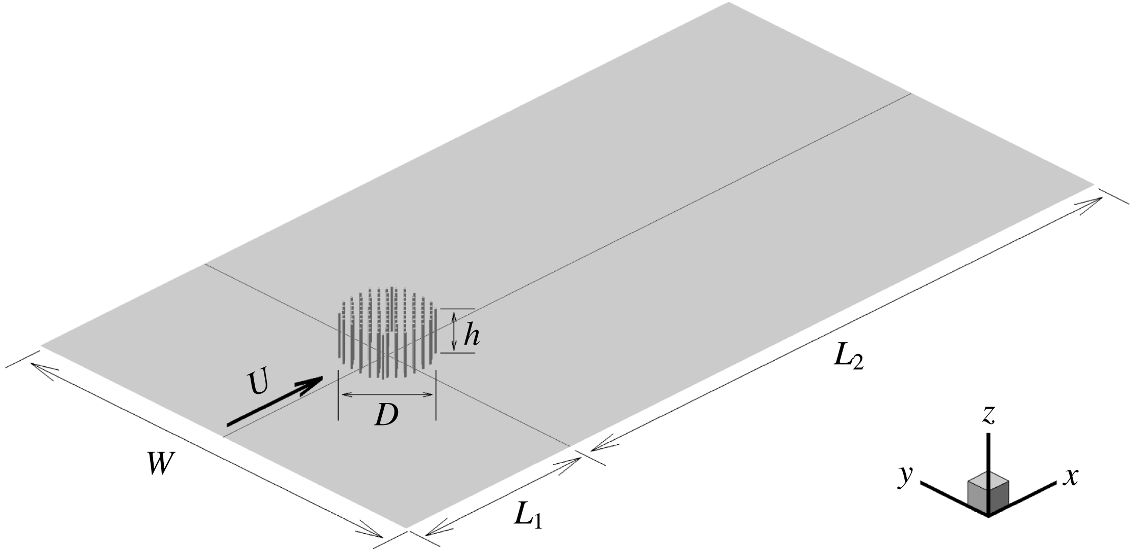
Sketch of the computational domain with a porous cylinder of diameter  $D$ containing a number of solid cylinders of diameter  $d$ . The domain size in the horizontal plane is the same in the flat-bed and deformed-bed cases.

The horizontal set-up of the present numerical simulations (figure 1) is similar to that used in the related study of Chang & Constantinescu (Reference Chang and Constantinescu2015). In the present flat-bed simulations, the bed is located at $z=0$ and the free surface at $z=h$ . The origin of the system of coordinates is located at the centre of the porous or solid cylinder. The streamwise direction is $x$ , while the spanwise direction is $y$ . The simulations with $\text{SVF}=0.034$ and $\text{SVF}=0.092$ are conducted with the same flow conditions and geometrical set-up (e.g. number of cylinders in the array, $d/D$ , $h/D$ , $Re_{D}$ ) as those considered in the corresponding experiments of Follett & Nepf (Reference Follett and Nepf2012). 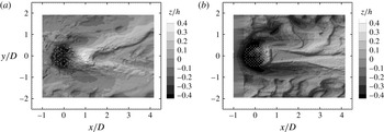In the deformed-bed simulations, $z=0$ corresponds to the bed level away from the porous cylinder, where the bed deformations are negligible during the erosion and deposition process. The shape of the deformed bed at equilibrium scour conditions (figure 2) is obtained from the corresponding loose-bed experiments (experimental cases 7 and 15) conducted by Follett & Nepf (Reference Follett and Nepf2012). The width of the computational domain is $W\approx 6D$ , approximately the same as the width of the flume in the experiments ( $D=0.22$  m cases) conducted by Follett & Nepf (Reference Follett and Nepf2012). The distance between the inflow and the centre of the porous cylinder is $L_{1}\approx 2.5D$ and the distance between the centre of the porous cylinder and the exit section is $L_{2}\approx 7D$ (figure 1). The solid cylinders forming the array are placed using a close-to-regular staggered pattern in the $x{-}y$ planes (see also Chang & Constantinescu Reference Chang and Constantinescu2015). A small random displacement of $0.5d{-}1.0d$ is applied on the initial regular pattern to reduce the regularity of the wake-to-wake interactions between neighbouring cylinders. This arrangement is similar to the one used in laboratory experiments of such flows (e.g. see Chen et al. Reference Chen, Ortiz, Zong and Nepf2012; Zong & Nepf Reference Zong and Nepf2012). In most of the simulations, the horizontal mesh contains close to one million cells and 48 points are used to resolve the flow in the vertical direction. The mesh is refined inside the porous cylinder region and some distance downstream of it. In the vertical direction, the mesh is refined close to the bed surface. The first point off the bed surface is situated at approximately $0.0005h$ ( ${\approx}0.00025D$ ) from the bed.

Figure 2.

Equilibrium scour bathymetry in the deformed-bed cases with (a)  $\text{SVF}=0.034$ and (b)  $\text{SVF}=0.092$ , as measured in the experiments of Follett & Nepf (Reference Follett and Nepf2012). The contours show the non-dimensional bed elevation $z/h$ , where $z=0$ corresponds to the initial horizontal bed elevation at the start of the scour and deposition process.

The velocity fields containing resolved turbulent fluctuations at the inflow section are obtained from precursor LES simulations performed in a straight channel with periodic boundary conditions in the streamwise direction (Kirkil & Constantinescu Reference Kirkil and Constantinescu2009, Reference Kirkil and Constantinescu2010). The flow depth, channel width and channel Reynolds number in the precursor simulation are the same as in the corresponding domain containing the porous or solid cylinder. A convective boundary condition is used at the outflow (Rodi et al. Reference Rodi, Constantinescu and Stoesser2013). The free surface is modelled as a shear-free rigid lid. This is justified due to the low value of the channel Froude number ( $Fr=U/(gh)^{1/2}<0.3$ , where $g$ is the gravitational acceleration) and small free-surface deformations observed in the corresponding experiments. One should also mention that in cases where organic matter or surfactant films are present at the free surface, use of a no-slip boundary condition at the free surface is more appropriate (Cuenot, Magnaudet & Spennato Reference Cuenot, Magnaudet and Spennato1997). However, that was not the case in the experiments based on which the numerical test cases were set up in the present study. All of the solid surfaces were treated as no-slip walls. The channel bottom was treated as a rough surface with an equivalent roughness height $k_{s}=1.0$  mm, which corresponds to two times the median sand grain diameter used in the experiments. The mean value of the bed friction velocity in the incoming flow can be used to estimate a friction factor. The estimated value of the friction factor in the different test cases ( $f\approx 0.027$ ) is very close to the value obtained using the Moody diagram for the same channel Reynolds number and relative roughness height. The time step is $0.001D/U$ . This low value allows resolution of the range of energetic frequencies associated with the dynamically important coherent structures in the flow (e.g. necklace vortices, vortex shedding in the wake of the solid cylinders, vortex tubes in the SSLs of the porous cylinder). A grid dependency study was conducted for the flat-bed case with $\text{SVF}=0.092$ to confirm that the mean flow and turbulence statistics were close to grid-independent. Mean flow and turbulence statistics were collected over a time interval of approximately $80D/U$ . This time interval was sufficiently long to converge the first- and second-order statistics.

In the case of circular cylinders, $a=Nd/(\unicode[STIX]{x03C0}D^{2}/4)$ and $\text{SVF}=Nd^{2}/D^{2}$ , which means that $aD=\text{SVF}\ast (D/d)\ast 4/\unicode[STIX]{x03C0}$ . Thus, when comparing cases with the same value of $D/d$ , investigating the effects of varying $aD$ and SVF is equivalent. The inverse of this variable, $1/(aD)$ , is a non-dimensional length scale which, together with $d/D$ , characterizes the porous patch and controls the total drag force induced by the patch. In the present simulations, $0.03<\text{SVF}<0.23$ , $1.4<aD<9.6$ and $0.03<d/D<0.06$ . This range is comparable to that used in laboratory experiments of flow past patches of vegetation. For example, $0.03\leqslant \text{SVF}\leqslant 0.36$ , $0.1<aD<8.0$ , $0.014\leqslant d/D\leqslant 0.05$ in the experiments of Zong & Nepf (Reference Zong and Nepf2012), $0.03<\text{SVF}<0.51$ , $0.7<aD<9$ , $0.015<d/D<0.128$ in the experiments of Chen et al. (Reference Chen, Ortiz, Zong and Nepf2012), $0.03<\text{SVF}<0.1$ , $1.3<aD<4.4$ , $d/D=0.03$ in the experiments of Follett & Nepf (Reference Follett and Nepf2012). The numerical study of Chang & Constantinescu (Reference Chang and Constantinescu2015) for long porous cylinders was conducted with $0.023<\text{SVF}<0.2$ , $0.61<aD<5.5$ , $0.048<d/D<0.096$ .

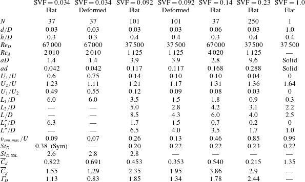
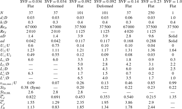
The main geometrical and flow parameters of the six test cases are reviewed in table 1. Also included are results for the limiting case of flow past a solid cylinder ( $\text{SVF}=1.0$ ) placed on a flat bed. In all cases, $D=0.22$  m. Most of the simulations are conducted with $3.5\times 10^{4}<Re_{D}<7.0\times 10^{4}$ , $480<Re_{d}<960$ and $d=0.03D$ . The channel Reynolds number is larger than 15 000 for all cases.

Flat-bed simulations with $d=0.03D$ and $\text{SVF}=0.034$ , 0.092, 0.14 and 0.23 are used to study the effect of the SVF and $aD$ on the flow. The effect of the relative size of the solid cylinders, $d/D$ , is investigated by comparing the flat-bed simulations ( $N=37$ ) with $\text{SVF}=0.034$ ( $d/D=0.03$ ) and $\text{SVF}=0.14$ ( $d/D=0.06$ ). Two of the test cases ( $\text{SVF}=0.034$ and $\text{SVF}=0.092$ ) are also run with a deformed bed corresponding to equilibrium scour conditions, as measured in the corresponding loose-bed experiments conducted by Follett & Nepf (Reference Follett and Nepf2012). As shown in figure 2, the SVF has a significant effect on the bathymetry shape at equilibrium. While in the $\text{SVF}=0.034$ case, a mound of sediment forms immediately behind the porous cylinder and most of the erosion takes place inside the array, in the $\text{SVF}=0.092$ case, no significant erosion takes place in a triangular region at the back of the porous cylinder, two regions of sediment deposition form starting around the downstream end of this triangular region and significant erosion occurs not only inside the upstream part of the porous cylinder but also around the lateral sides of the porous cylinder. Comparison of the flat-bed and deformed-bed simulations allows investigation of the changes in the flow structure associated with the bed evolution during the erosion and deposition process.

Table 1.

The main geometrical and flow variables of the test cases. Here, $N$ is the number of cylinders in the array; $d$ is the diameter of the solid cylinders; $D$ is the diameter of the circular array; $Re_{D}=UD/\unicode[STIX]{x1D708}$ ; $Re_{d}=Ud/\unicode[STIX]{x1D708}$ ; $aD$ is the non-dimensional frontal area per unit volume for the array; $U_{1}$ is the centreline streamwise velocity at the upstream end of the steady wake region; $U_{2}$ is the maximum streamwise velocity of the flow on the sides of the array; $L_{1}$ , $L_{1}^{\prime \prime }$ are estimates of the steady wake length; $L$ , $L^{\prime \prime }$ are estimates of the total wake length; $L_{2}=L-L_{1}$ ; $v_{rms,max}$ is the maximum of the r.m.s. of the lateral velocity fluctuations along the centreline; $St_{D}$ is the Strouhal number defined with $U$ and $D$ corresponding to the most energetic frequency in the wake of the (porous) cylinder; $St_{D,SSL}$ is the Strouhal number defined with $U$ and $D$ corresponding to the energetic eddies shed close to the upstream end of the SSLs of the porous cylinders; $\overline{C}_{d}$ is the mean solid cylinder streamwise drag coefficient for the array defined with the incoming velocity, $U$ , as velocity scale; $\overline{C}_{d}^{\prime }$ is the mean solid cylinder streamwise drag coefficient for the array defined with the mean velocity inside the porous cylinder, $U_{p}$ , as velocity scale; $\unicode[STIX]{x1D6E4}_{D}=\overline{C}_{d}aD/(1-\text{SVF})$ is a combined drag parameter for the array.

Figure 3.

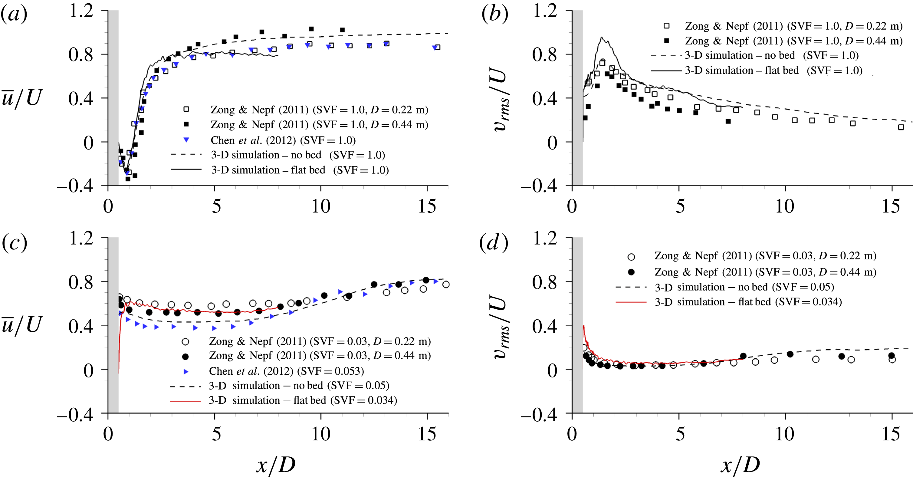
Longitudinal profiles of the streamwise velocity, $\overline{u}/U$ , and the r.m.s. of the lateral velocity fluctuations, $v_{rms}/U$ , measured along the centreline, $y/D=0$ , close to the free surface. The grey region denotes the solid or porous cylinder. Panels (a,b) compare the present flat-bed 3-D simulation, the 3-D simulation of Chang & Constantinescu (Reference Chang and Constantinescu2015) for a long cylinder (no bed) and the experiments of Zong & Nepf (Reference Zong and Nepf2011) and Chen et al. (Reference Chen, Ortiz, Zong and Nepf2012) for the solid cylinder ( $\text{SVF}=1$ ) case. Panels (c,d) compare the present flat-bed 3-D simulation with $\text{SVF}=0.034$ and $d/D=0.03$ , the 3-D simulation of Chang & Constantinescu (Reference Chang and Constantinescu2015) for a long cylinder (no bed) with $\text{SVF}=0.05$ and $d/D=0.05$ , and the experiments of Zong & Nepf (Reference Zong and Nepf2011) and Chen et al. (Reference Chen, Ortiz, Zong and Nepf2012) performed for $\text{SVF}=0.03$ and $\text{SVF}=0.053$ respectively. The two sets of experimental data from Zong & Nepf (Reference Zong and Nepf2011) correspond to different diameters of the porous cylinder ( $D=0.22$  m,  $d/D=0.027$ and $D=0.42$  m,  $d/D=0.015$ ).

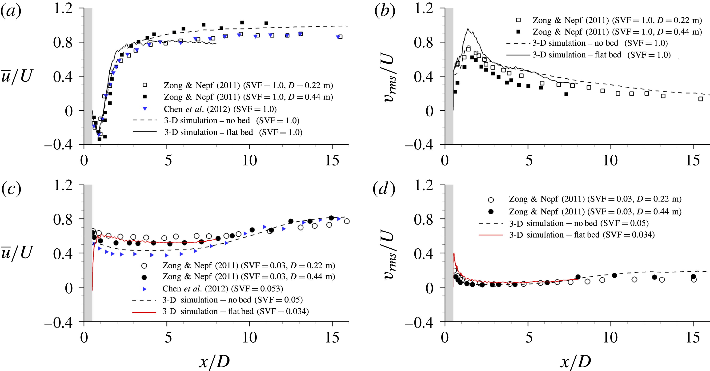
Figure 3 shows validation results for the simulations conducted with $\text{SVF}=1.0$ and $\text{SVF}=0.034$ (see also table 1). The longitudinal profiles of the streamwise velocity, $\overline{u}/U$ , and the r.m.s. of the lateral velocity fluctuations, $v_{rms}/U$ , along the centreline of the solid/porous cylinder are compared for the present simulations, the 3-D LES of flow past a long cylinder conducted by Chang & Constantinescu (Reference Chang and Constantinescu2015), and the experimental measurements of Zong & Nepf (Reference Zong and Nepf2011) and Chen et al. (Reference Chen, Ortiz, Zong and Nepf2012). The comparison for the solid cylinder case (figure 3 a) shows that the predicted centreline velocity is the present simulation is in good agreement with the experimental data measured by Zong & Nepf (Reference Zong and Nepf2011) and Chen et al. (Reference Chen, Ortiz, Zong and Nepf2012) for a cylinder of equal size ( $D=0.22$  m). Comparison with the case of a long cylinder shows that the presence of the bed and free surface delays the recovery of the mean streamwise velocity in the wake towards the free-stream value. The values of $v_{rms}/U$ along the centreline are overpredicted by the present simulation around $x/D=1.5$ (figure 3 b). It is probable that the main reason is the relatively high level of turbulence intensity present in the incoming flow which is assumed to be fully turbulent in our simulation. The long-cylinder simulation is performed with no incoming turbulence, while in the experiments, the flume length was probably not sufficiently long to ensure fully developed turbulent flow at the location of the porous cylinder. However, the agreement with both the experimental data of Zong & Nepf (Reference Zong and Nepf2012) for the $D=0.22$  m case and the LES of a long cylinder is very good for $x/D>2$ . One should also mention that the predicted value of the mean drag coefficient for the solid cylinder is $\overline{C}_{d}=1.35$ , slightly larger than the value predicted by the long-cylinder simulation ( $\overline{C}_{d}=1.17$ ). Kirkil & Constantinescu (Reference Kirkil and Constantinescu2015) observed a similar increase of the mean drag coefficient on a solid cylinder once flow shallowness effects become non-negligible (e.g. $D/h\approx 2$ in the present simulation conducted for moderately shallow flow conditions). Most of the increase is due to the bottom boundary layer, which reduces the incoming flow velocity around the bottom part of the cylinder. For such conditions, the drag coefficient assumes larger values. Despite differences in $Re_{D}$ , $d/D$ , $D/h$ and $N$ among the different cases with $0.03<\text{SVF}<0.05$ compared in figures 3(c) and 3(d), the agreement between the present simulation results and the other experimental and numerical data represented in these figures is very satisfactory.

Figure 4.

Visualization of coherent structures using the $\unicode[STIX]{x1D64C}$ criterion: (a)  $\text{SVF}=0.092$ , 3-D view; (b)  $\text{SVF}=0.092$ ; (c)  $\text{SVF}=0.092$ , deformed bed; (d)  $\text{SVF}=0.14$ ; (e)  $\text{SVF}=0.23$ ; (f)  $\text{SVF}=1$ . The $\unicode[STIX]{x1D64C}$ isosurface is coloured using the non-dimensional vertical position, $z/h$ . The red arrows in (d) point towards the necklace vortices forming around the upstream face of the solid cylinders directly exposed to the incoming flow.

3 Flow structure around the upstream face of the porous cylinder

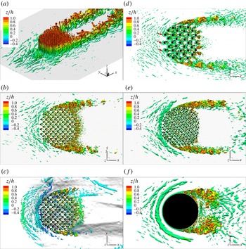
Figure 4(a) visualizes the vortical structure around the porous cylinder for the $\text{SVF}=0.092$ case using the $\unicode[STIX]{x1D64C}$ criterion (Dubief & Delcayre Reference Dubief and Delcayre2000). The quantity $\unicode[STIX]{x1D64C}$ is the second invariant of the resolved velocity gradient tensor ( $\unicode[STIX]{x1D64C}=-0.5\unicode[STIX]{x2202}u_{i}/\unicode[STIX]{x2202}x_{j}\ast \unicode[STIX]{x2202}u_{j}/\unicode[STIX]{x2202}x_{i}(D^{2}/U^{2})$ ). As for the case of a long porous cylinder, large-scale coherent structures in the form of deformed vortex tubes are generated in the SSLs of the surface-mounted porous cylinder. However, large-scale coherent structures are also present in the near-bed region around the upstream base of the porous cylinder. These eddies are induced by the adverse pressure gradients present in the vicinity of the bottom boundary layer. Similarly to the case of a surface-mounted solid cylinder, adverse pressure gradients are generated by the interaction of the incoming flow with the solid cylinders in the array directly or partially exposed to the incoming flow. This interaction results in partial lateral deflection of the incoming flow approaching the porous cylinder, as also observed for long cylinders (Chang & Constantinescu Reference Chang and Constantinescu2015), and in the formation of a vertical downflow fairly parallel to the upstream face of the porous cylinder (see the discussion of figure 11). As it reaches the bed, most of the downflow is diverted upstream. One difference from the corresponding case of a solid cylinder is that the downflow can slightly penetrate inside the porous cylinder as it moves towards the bed surface.

As the SVF increases, the bleeding flow becomes weaker, the adverse pressure gradients generated around the porous cylinder increase and the downflow becomes stronger. Thus, for a sufficiently large SVF, necklace vortices should start to form around the upstream base of the cylinder, as is the case for the widely studied case of a solid cylinder mounted on a flat surface (figure 4 f). Indeed, a necklace vortex is present in the $\text{SVF}=0.23$ case (figure 4 e), although its strength (e.g. as measured by the circulation of its core) is smaller than that of the corresponding main necklace vortex observed in the $\text{SVF}=1$ case. Secondary necklace vortices which are detaching from the region where the incoming boundary layer separates and eventually merge in an irregular way with the main necklace vortex are also observed in figures 4(e) and 4(f). No well-defined necklace vortex is observed in the $\text{SVF}=0.034$ , $\text{SVF}=0.092$ (figure 4 b) and $\text{SVF}=0.14$ (figure 4 d) flat-bed cases. Elongated eddies form around part of the upstream base of the cylinder in the $\text{SVF}=0.092$ case, but these streaky structures never generate a necklace vortex. Small necklace vortices also form around the base of the solid cylinders directly exposed to the flow for cases when no necklace vortex forms around the base of the porous cylinder. These vortices are nicely captured in figure 4(d) for the $\text{SVF}=0.14$ ( $d/D=0.06$ ) case. The orientation of the legs of these necklace vortices follows that of the mean flow approaching the individual cylinders in the array. This is why the legs of these necklace vortices are sometimes oriented at a large angle relative to the streamwise direction in figure 4(d). These necklace vortices are a main mechanism for development of scour around the solid cylinders exposed to the incoming flow. Depending on the spacing and the SVF, the scour holes developing around the individual solid cylinders can coalesce. This creates the conditions for the formation of a scour hole around the upstream base of the cylinder even for cases when no necklace vortices form around the porous cylinder.

In the case of a loose bed, scour develops around the sides and upstream face of the cylinder if the SVF is sufficiently high. The presence of a scour hole favours the formation of necklace vortices and stabilizes their position relative to the upstream face of the (porous) cylinder. This is one of the reasons why, once the scour hole becomes sufficiently deep, the necklace vortices rather than the flow acceleration on the sides of the (porous) cylinder drive the growth of the scour hole around the upstream base of the (porous) cylinder. For example, while in the $\text{SVF}=0.092$ flat-bed case, no necklace vortices are present (figure 4 b), in the $\text{SVF}=0.092$ case with equilibrium scour bed (figure 4 c), a necklace vortex is present close to the junction line between the porous cylinder and the bed. Additionally, the incoming boundary layer separates close to the upstream mouth of the scour hole and a small recirculation region forms. Small necklace vortices are shed irregularly from this region towards the porous cylinder, similarly to the scenario observed for solid cylinders (Kirkil et al. Reference Kirkil, Constantinescu and Ettema2009).

Figure 5.

Effect of the solid volume fraction on the mean flow structure in front of the porous cylinder. The distributions of the TKE, $k/U^{2}$ (left-hand side) and out-of-plane mean vorticity magnitude, $|\unicode[STIX]{x1D714}_{y}D|/U$ (right-hand side), are shown in a vertical $x{-}z$ plane situated close to the symmetry plane ( $y=0.7d$ ); (a)  $\text{SVF}=0.092$ ; (b)  $\text{SVF}=0.23$ ; (c)  $\text{SVF}=1.0$ ; (d)  $\text{SVF}=0.092$ , deformed bed. The solid cylinders are shown in grey. The vertical dashed line corresponds to the boundary of the porous cylinder ( $x/D=-0.5$ ). In some of the cases, the vertical $x{-}z$ plane does not intersect the solid cylinders situated close to the face of the porous cylinder.

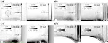
The distribution of the TKE, $k/U^{2}$ , in an $x{-}z$ vertical plane situated close to the symmetry plane (see the inset in figure 5) allows assessment of the effect of the eddies advected with the downflow on the amplification of the turbulence in the near-bed region around the upstream base of the porous cylinder. Even though the 2-D streamlines in figure 5(a) show that the mean flow does not separate, a region where the TKE is strongly amplified compared with the levels in the approaching fully developed turbulent flow is present in the $\text{SVF}=0.092$ case. The TKE amplification is induced by the formation of larger-scale eddies in the near-bed region (figure 4 b), where the bottom boundary layer is subject to adverse pressure gradients, and eddies advected with the downflow reach the bed surface. However, this region does not contain strongly coherent necklace vortices, as observed from the distributions of both the 2-D streamline patterns and the out-of-plane mean vorticity in figure 5(a). In contrast, in the $\text{SVF}=0.23$ case (figure 5 b), the region of high vorticity close to the bed contains two patches of large vorticity next to the porous cylinder, and the incoming boundary layer separates at approximately 0.2D from the face of the porous cylinder. The largest patch of high vorticity corresponds to the main necklace vortex, which is present at all times in the instantaneous flow fields. Its strength (circulation), position and mean size are variable in time. A very significant increase is observed in the size of the region of high TKE, and the peak TKE values inside this region, as the SVF increases from 0.092 to 0.23. This increase is mainly due to the oscillations of the core of the main necklace vortex in the $\text{SVF}=0.23$ case. As the SVF is further increased, the coherence of the main necklace vortex continues to increase and a secondary vortex forms upstream of the main necklace vortex (e.g. see the results for $\text{SVF}=0.23$ and $\text{SVF}=1.0$ in figures 5 b and 5 c respectively). The size of the patch of vorticity associated with the core of the main necklace vortex, and the peak TKE values inside the core of this vortex increase by close to 100 % as the SVF increases from 0.23 to 1.0. Moreover, the location where the incoming boundary layer separates moves upstream, to approximately $0.35D$ from the cylinder in the $\text{SVF}=1.0$ case.

The development of a naturally deformed scoured bed favours the formation of a necklace vortex over the deepest part of the scour hole (see the vorticity distribution in figure 5 d), even for cases when a necklace vortex is not present at the start of the scouring process (e.g. the $\text{SVF}=0.092$ case). Given that, in such cases, patches of vorticity separate fairly regularly from the downstream end of the attached boundary layer at the upstream mouth of the scoured region, the region of high TKE covers all of the scoured region in between the attached boundary layer and the porous cylinder (figure 5 d).

Figure 6.

The non-dimensional pressure distribution in the mean flow close to the free surface ( $z/h=0.9$ ) and close to the bed ( $z/h=0.1$ ) in the flat-bed cases with (a)  $\text{SVF}=0.092$ , (b)  $\text{SVF}=0.23$ and (c)  $\text{SVF}=1.0$ .

Figure 7.

The non-dimensional vertical vorticity distribution in the instantaneous flow close to the free surface ( $z/h=0.9$ ): (a)  $\text{SVF}=0.034$ ; (b)  $\text{SVF}=0.092$ ; (c)  $\text{SVF}=0.092$ , deformed bed; (d)  $\text{SVF}=0.14$ ; (e)  $\text{SVF}=0.23$ . Regions with $|\unicode[STIX]{x1D714}_{z}D/U|<1$ were blanked.

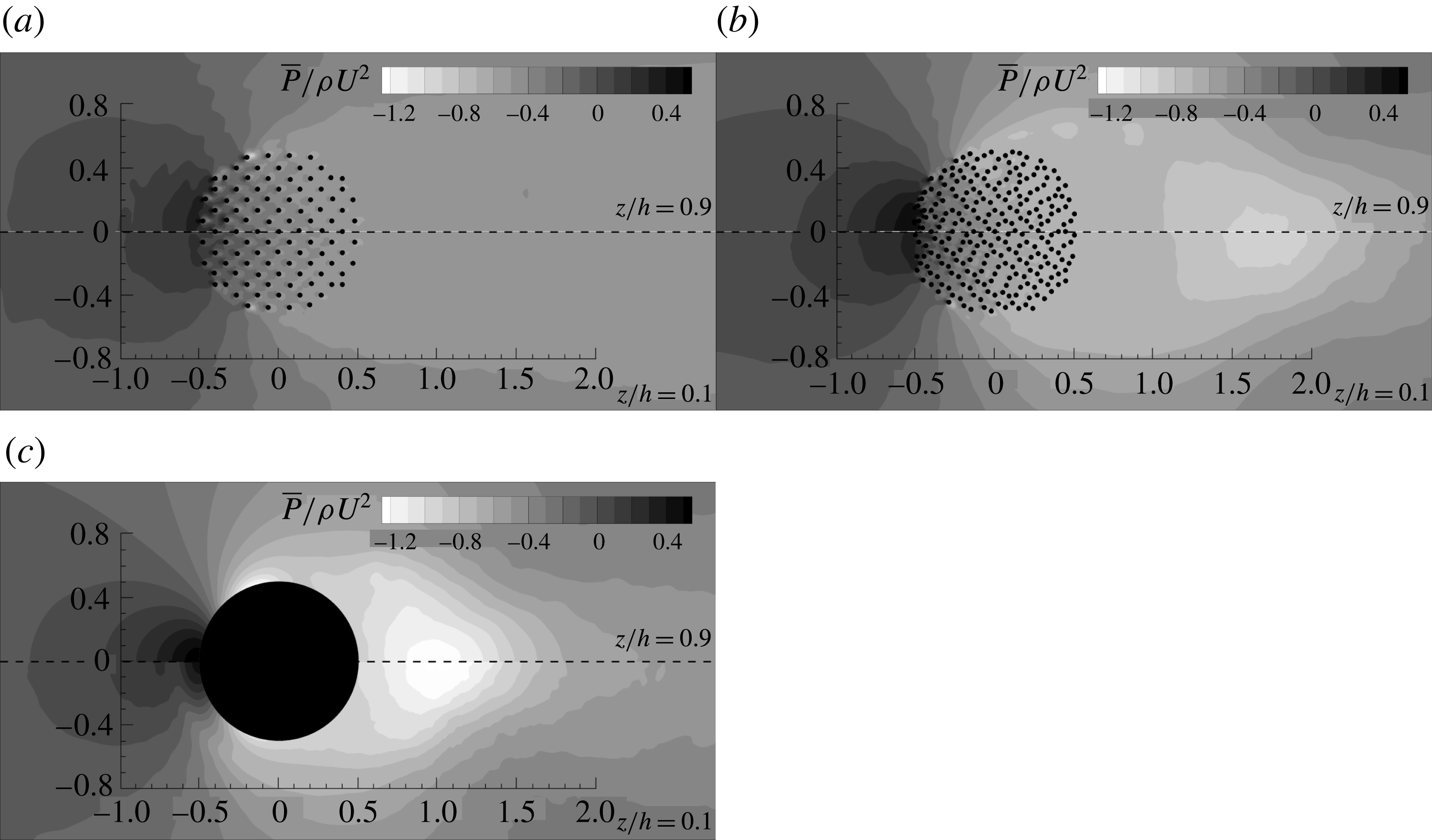
In the previous discussion, we made the point that the adverse pressure gradients generated in front of the (porous) cylinder increase monotonically with increasing SVF. This is illustrated in a quantitative way in figure 6, where the mean pressure distribution, $\overline{p}/\unicode[STIX]{x1D70C}U^{2}$ , is represented in two horizontal planes situated near the free surface ( $z/h=0.9$ , top half of figure 6) and near the bed ( $z/h=0.1$ ) for the $\text{SVF}=0.092$ , 0.23 and 1.0 cases. For all cases, the adverse pressure gradients are weaker close to the bed and the vertical non-uniformity effects increase with increasing SVF. This occurs because the mean incoming velocity decreases as the bed surface is approached. Moreover, the decay of the pressure away from the upstream face of the porous cylinder is faster for the cases with higher SVFs. Moreover, for the same SVF, the streamwise pressure gradient inside the porous cylinder is smaller near the bed compared with close to the free surface. This is due to the increased strength of the bleeding flow and the increased penetration of the downflow inside the porous cylinder with decreasing SVF. Vertical non-uniformity effects become weaker as the SVF decreases. The results in figure 6 also show that vertical non-uniformity effects on the mean pressure distribution behind the porous cylinder are fairly negligible.

4 Flow and turbulence structure inside the porous cylinder and its wake

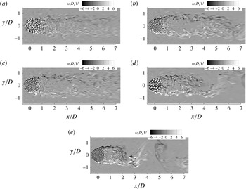
The distributions of the instantaneous vertical vorticity in the $z/h=0.9$ plane in figure 7 show that important differences are observed in the near-wake structure close to the free surface between cases with low and high SVFs, and also between high-SVF cases with flat and deformed beds. For the flat-bed cases with high SVFs (e.g. $\text{SVF}=0.24$ , 0.14 and 0.092 in figure 7), counter-rotating wake billows are shed at the back of the porous cylinder, and the vortex shedding is asymmetrical, similarly to the von Kármán vortex street observed past long solid cylinders. This is expected, as for all cases considered in the present study, the wake stability number is much larger than 0.2, so the effects of bed friction on the formation of the wake billows are relatively small. As for the case of long porous cylinders (Chang & Constantinescu Reference Chang and Constantinescu2015), the SSLs of the porous cylinder become longer and the distance from the back of the cylinder to the location at which wake billows form increases with decreasing SVF. For example, the wake billows form at approximately 0.7D and 4.0D from the back of the cylinder in the $\text{SVF}=0.23$ and $\text{SVF}=0.092$ cases respectively. The Strouhal number, $St_{D}=fU/D$ (where $f$ is the frequency), associated with the formation and advection of wake billows increases slightly with increasing SVF until $\text{SVF}\approx 0.23$ (e.g. from 0.2 for $\text{SVF}=0.092$ to approximately 0.23 for $\text{SVF}=0.23$ ; see also table 1). For very high SVFs, the Strouhal number decreases slightly (e.g. $St_{D}\approx 0.22$ for $\text{SVF}=1.0$ ). The trend and range of $St_{D}$ values are consistent with those predicted for long cylinders by Chang & Constantinescu (Reference Chang and Constantinescu2015).

Even if the SSLs of the porous cylinder are still populated by energetic coherent structures originating mostly from the wakes of the solid cylinders situated close to the lateral sides of the porous cylinder (polar angles measured for the symmetry plane $|\unicode[STIX]{x1D719}|\approx 90^{\circ }$ ), the antisymmetric vortex shedding in the wake is supressed in the $\text{SVF}=0.034$ case (figure 7 a). This is because the bleeding flow entering the region situated in between the two SSLs at the back of the porous cylinder is sufficiently strong to impede the natural interactions of the two SSLs, which results in the formation of wake billows. Still, the wake contains larger-scale eddies which form mostly via merging of the co-rotating vortex-tube-like eddies advected in each SSL. At large distances from the porous cylinder ( $x/D>4$ ), the Strouhal number associated with the passage of these eddies is close to 0.38 in the $\text{SVF}=0.034$ case. Another interesting observation is that a very energetic frequency is present inside the upstream part of the SSLs in the $\text{SVF}=0.034$ case. The corresponding Strouhal number, $St_{D,SSL}$ , is around 2.6–2.8 (table 1). It corresponds to the frequency of passage of eddies shed in the wake of the solid cylinders which are injected into the upstream part of the SSL. This frequency is also present in the $\text{SVF}=0.092$ case for which the antisymmetrical vortex shedding mode is present.

For the moderately shallow flow conditions considered in the present study ( $D/h\approx 2$ ) and for sufficiently high SVFs, another important change in the wake structure occurs during the later stages of the scour and erosion process. Once the scour hole on the side of the porous cylinder becomes sufficiently large and a region of flow deposition forms close to the symmetry plane some distance behind the porous cylinder, an upwelling mean flow motion is induced close to the symmetry plane at the back of the porous cylinder (e.g. see the detailed discussion in Kirkil et al. (Reference Kirkil, Constantinescu and Ettema2009) for the case of a solid cylinder with $D/h\approx 1$ ). The upwelled fluid is diverted away from the symmetry plane as it approaches the free surface. This is another mechanism that impedes the interactions of the SSLs, which results in antisymmetrical shedding of wake billows. In the $\text{SVF}=0.092$ case with a deformed equilibrium scour bed, a weak upwelling motion is present behind the cylinder. This upwelling is weaker than the one observed for solid cylinders, but it is strong enough to weaken the antisymmetric mode considerably (figure 7 c). The $St_{D}=0.22$ frequency observed in the flat-bed case is still present in velocity spectra inside the near wake (not shown), but it is much less energetic in the deformed-bed case. Additionally, a range of energetic frequencies ( $0.125<St_{D}<0.4$ ) are present in the deformed-bed case. Therefore, the $\text{SVF}=0.092$ case with a deformed bed can be classified as a case with weak antisymmetric vortex shedding. Kirkil et al. (Reference Kirkil, Constantinescu and Ettema2009) observed total suppression of the antisymmetric mode and a transition to the symmetric mode for the case of a solid cylinder under similarly shallow conditions. For the relatively shallow conditions considered in the present study, the absence of a strong antisymmetric mode at the free surface can be used to infer the presence of a highly scoured bed surface in the cases with relatively high SVFs. However, for much deeper cases, the antisymmetric mode is expected to be present close to the free surface even for cases where the bathymetry is close to equilibrium conditions.

The development of scour inside the porous region and downstream of it affects the wake dynamics even for cases with low SVFs, where the symmetric vortex shedding mode is present for flat-bed conditions. For example, in the $\text{SVF}=0.034$ deformed-bed case, the velocity power spectra contain a range of energetic frequencies ( $0.12<St_{D}<0.8$ ), but no dominant frequency corresponding to the peak frequency $St_{D}=0.38$ associated with the symmetric shedding in the flat-bed simulation. On the other hand, the velocity spectra recorded at locations situated in the upstream part of the SSLs still contain a very energetic frequency ( $St_{D,SSL}=2.8$ ) which is fairly close to the value determined in the flat-bed case ( $St_{D,SSL}=2.6$ ).

Figure 8.

The non-dimensional TKE distribution close to the free surface ( $z/h=0.9$ ) and close to the bed ( $z/h=0.1$ ) in the flat-bed cases with (a)  $\text{SVF}=0.034$ , (b)  $\text{SVF}=0.092$ , (c)  $\text{SVF}=0.14$ , (d)  $\text{SVF}=0.23$ and (e)  $\text{SVF}=1.0$ . Regions with $|k/U^{2}|<0.03$ were blanked.

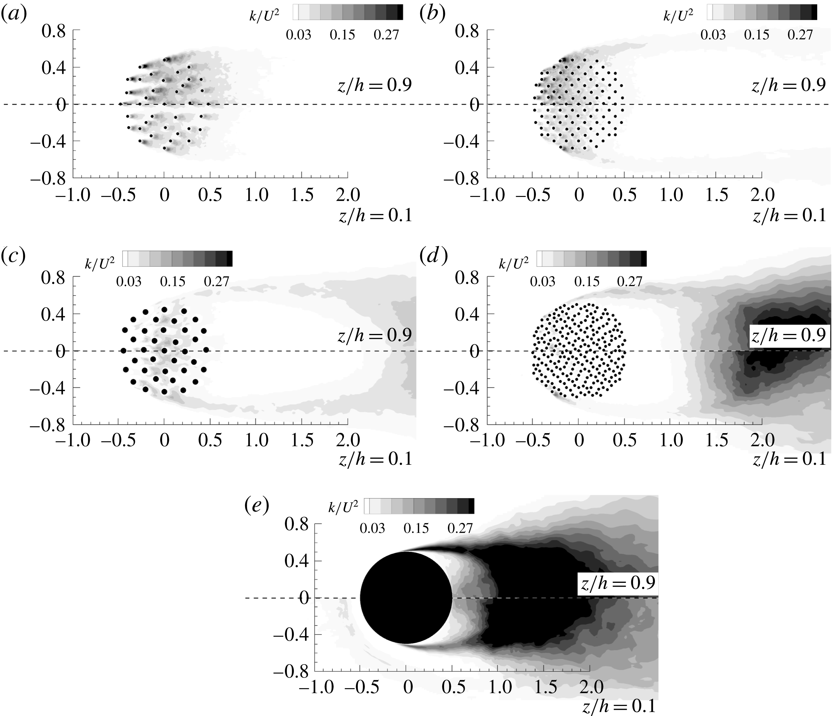
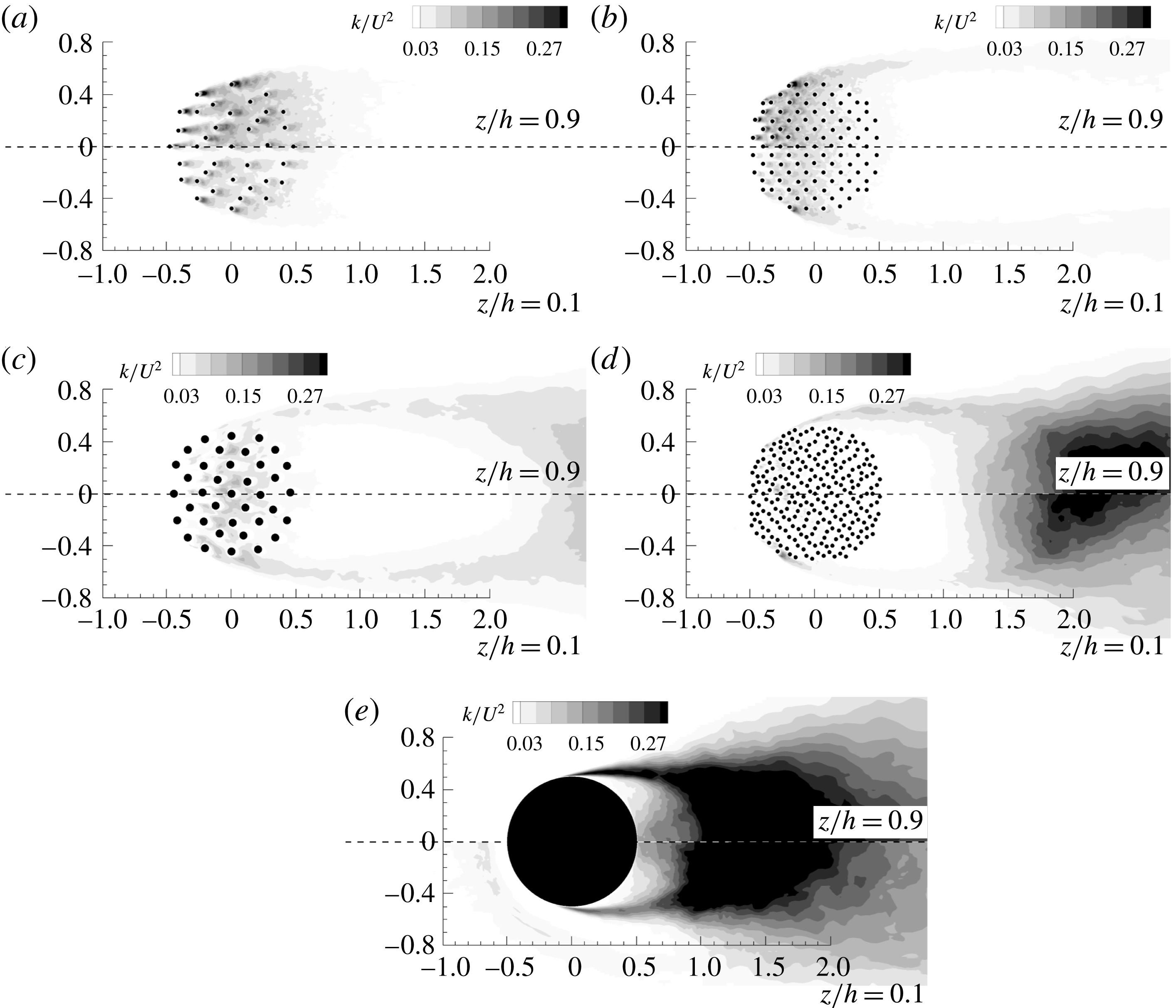
Figure 8 provides information on the vertical non-uniformity of the TKE distribution inside and close to the porous region for the flat-bed cases. At very low SVFs (e.g. $\text{SVF}=0.034$ in figure 8 a), the region of high TKE amplification induced by the interaction of the bleeding flow with the solid cylinders covers the whole porous region and some short distance behind it. As the SVF increases, the region of high TKE starts at the upstream face of the porous cylinder but does not cover the whole porous region (e.g. it ends at $x/D\approx 0.2$ for $\text{SVF}=0.092$ ; figure 8 b). This is because, as the SVF increases, the bleeding flow strongly decelerates as it interacts with the solid cylinders, and some of it changes orientation towards the sides of the cylinder. At even higher SVFs, the region of high TKE is situated away from the upstream and downstream ends of the porous region (e.g. it occupies roughly the region $-0.15<x/D<0.2D$ for $\text{SVF}=0.14$ ; figure 8 c). This occurs because the spacing between the cylinders becomes relatively small and the large-scale unsteady vortex shedding is significantly impeded around the most upstream cylinders in the array. In the $\text{SVF}=0.23$ case (figure 8 d), the region of high TKE shrinks even more and moves towards the front of the porous region ( $-0.3<x/D<0.1$ ). For very high SVFs, the bleeding flow is very weak and its interaction with the cylinders hardly generates large-scale eddies in their wakes (e.g. billow vortices). This is the case even for the cylinders for which the approaching flow velocity should be sufficiently high to generate strong unsteady shedding if the cylinder were situated far from the other cylinders.

Another noticeable effect of increasing the SVF in figure 8 is the increase of the TKE values inside the SSLs developing on the two sides of the porous cylinder. For $\text{SVF}>0.2$ , the TKE inside the upstream part of the SSLs becomes higher than the peak TKE values observed inside the porous region. The TKE distributions in figure 8 also show that the size of the region of high TKE, and the peak TKE values within this region decrease as the bed is approached. For most cases, the decay of the peak TKE values between $z/D=0.9$ and $z/D=0.1$ is of the order of 20 %. For the solid cylinder case (figure 8 e), the region of high TKE in front of the cylinder present in the $z/h=0.1$ plane corresponds to the core of the main necklace vortex. For cases with antisymmetric shedding, the patch of high TKE behind the porous cylinder corresponds to the region where wake billows form.

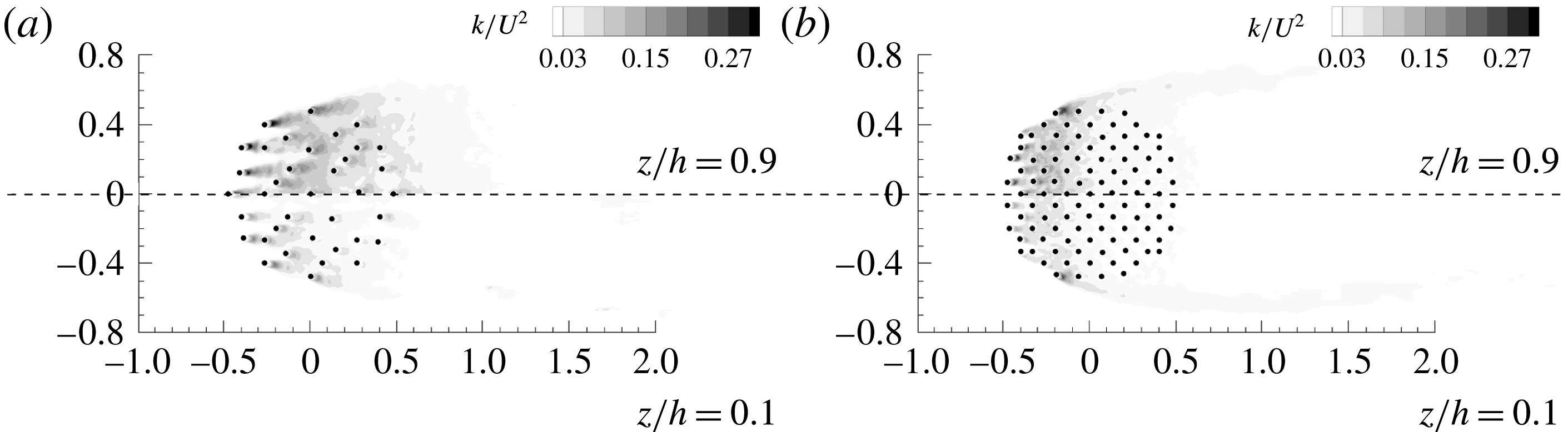
The TKE distributions near the free surface ( $z/D=0.9$ ) in the deformed-bed cases are qualitatively similar to those observed in the corresponding flat-bed cases (e.g. compare figures 8 a and 9 a for $\text{SVF}=0.034$ and figures 8 b and 9 b for $\text{SVF}=0.092$ ). For both SVFs, there is a reduction of the TKE levels within the region of high turbulence amplification of approximately 10 %–15 % in the deformed-bed case compared with the flat-bed case. A faster decay of the TKE is observed over the downstream part of the porous region in the deformed-bed cases, close to the free surface. The differences in the average TKE levels inside the region of high turbulence amplification increase to approximately 50 % if the comparison is made for a deformed surface situated at $0.1h$ from the bed. For the $\text{SVF}=0.092$ case, where the antisymmetric vortex shedding is greatly weakened at equilibrium scour conditions, the TKE values inside the SSLs are significantly lower in the deformed-bed case compared with the flat-bed case.

Figure 9.

The non-dimensional TKE distribution close to the free surface ( $z/h=0.9$ ) and close to the bed (on a deformed surface situated at a distance of $0.1h$ from the bed surface) in the deformed-bed cases with (a)  $\text{SVF}=0.034$ and (b)  $\text{SVF}=0.092$ . Regions with $|k/U^{2}|<0.03$ were blanked.

Figure 10.

The 2-D mean flow streamline patterns close to the free surface ( $z/h=0.9$ ) and close to the bed ( $z/h=0.1$ ) in the flat-bed cases with (a)  $\text{SVF}=0.034$ , (b)  $\text{SVF}=0.092$ , (c)  $\text{SVF}=0.23$ and (d)  $\text{SVF}=1$ .

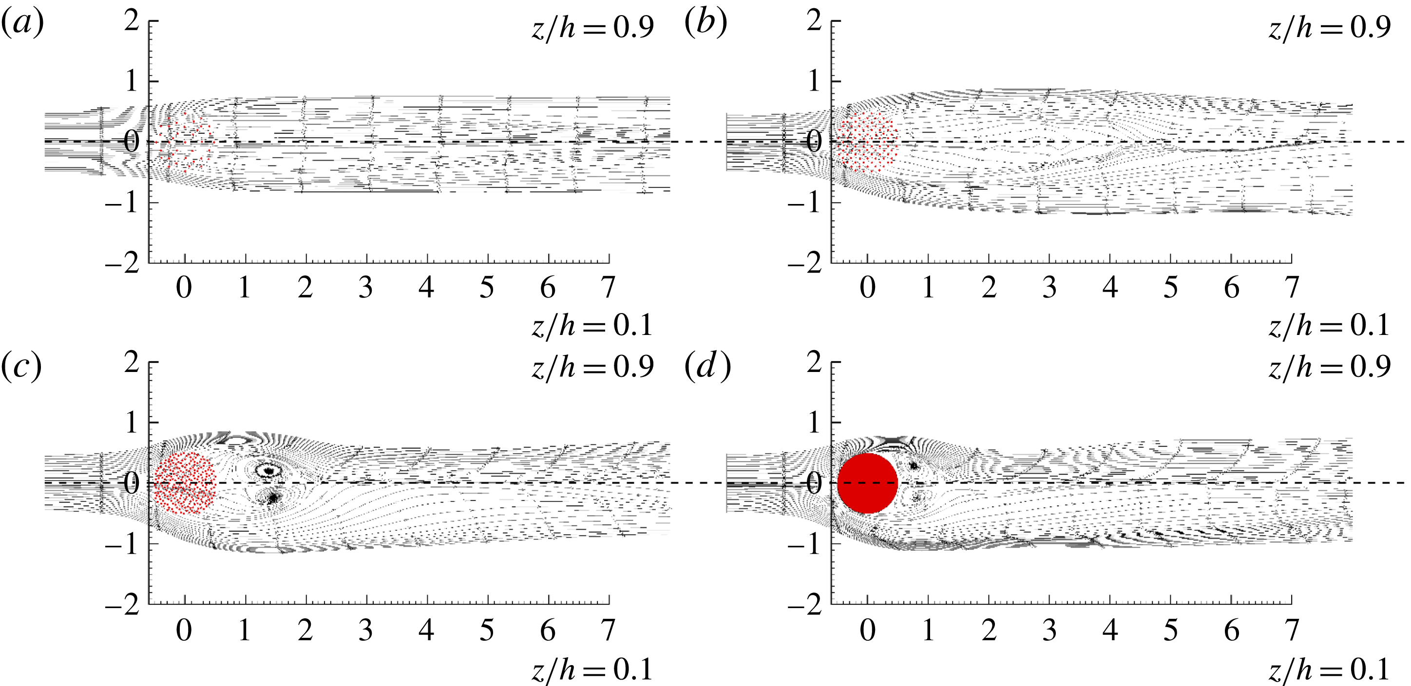
The presence of a recirculation bubble at the back of the cylinder in which the mean velocity and turbulence intensity are small provides a favourable habitat for fish and macroinvertebrates. In the flat-bed cases, no recirculation bubble forms for the low-SVF cases where the antisymmetric shedding mode is not present (e.g. $\text{SVF}=0.034$ in figure 10 a). For such cases, the lateral disturbance of the 2-D streamlines as they enter the wake region is minimal. The presence of a weak antisymmetric shedding mode does not automatically trigger the formation of a recirculation bubble, but the 2-D streamlines exiting the back of the porous region move first away from the symmetry plane and then back towards it before reorienting themselves along the streamwise direction (e.g. $\text{SVF}=0.092$ in figure 10 b). At higher SVFs, a recirculation eddy forms on each side of the wake with respect to the symmetry plane, but, as opposed to the limiting case of a solid cylinder (figure 10 d), this eddy does not touch the back of the (porous) cylinder. For example, this eddy extends between $x/D=1$ and $x/D=2$ in the $\text{SVF}=0.23$ case (figure 10 c). The predicted position and length of the recirculation eddy as a function of the SVF are consistent with those observed for long cylinders (Chang & Constantinescu Reference Chang and Constantinescu2015). The results in figure 10 show that the position and length of this eddy are fairly independent of the vertical location in the flat-bed simulations. Comparison of the 2-D streamline patterns inside the porous region in figure 10(a–c) shows that the bleeding flow inside the porous region is close to parallel to the streamwise direction only for very low SVFs. As the SVF increases, the streamlines entering the porous region are diverted laterally away from the symmetry plane. The bleeding flow exiting the porous region away from the symmetry plane has a strong lateral velocity component, which means that turbulent eddies advected with the bleeding flow will reach the SSLs. This dynamics directly affects the energy content and width of the SSLs.

In the previous section, we mentioned that part of the downflow penetrates into the upstream part of the porous region. This induces a secondary mean flow with a non-zero vertical velocity component in the flat-bed cases. The secondary flow present inside the patch and over part of the near wake has important implications for the capacity of plant stems to remove nutrients or to trap heavy metals and suspended particles (Zong & Nepf Reference Zong and Nepf2011; Follett & Nepf Reference Follett and Nepf2012). For example, particulates and matter are more likely to be deposited in regions where the secondary flow is oriented towards the bed and the mean flow parallel to the bed is weak. Several studies have shown that the upstream part of the wake behind an array of emerged rigid cylinders placed in a loose-bed open channel is a region where fine particle deposition is important (Follett & Nepf Reference Follett and Nepf2012). This means that this part of the wake is also a region that contains soil with high levels of nutrients which is favourable to new plant growth and may explain why patches grow mainly on the side of the steady wake region (Follett & Nepf Reference Follett and Nepf2012).

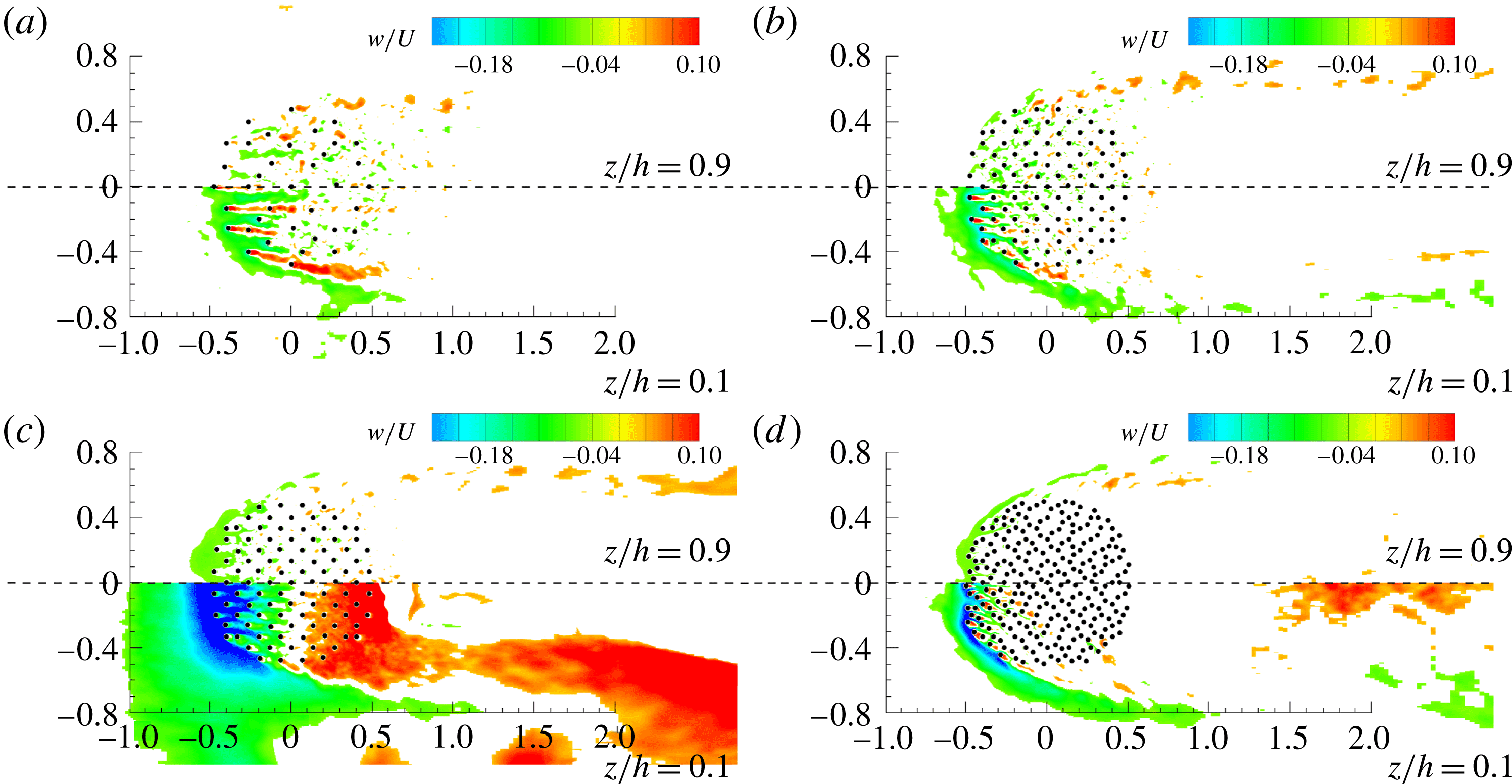
As expected, the mean vertical velocity component is fairly small close to the free surface. However, as the bed is approached (e.g. see the distributions on a surface situated at $0.1h$ from the bed in figures 11 a,b and 11 d), one can see a region of negative (towards the bed) vertical velocities developing around the upstream face of the porous cylinder. This region of negative velocities penetrates inside the porous patch and occupies the main ‘corridors’ in between the solid cylinders. The length of the region of negative vertical velocities inside the porous cylinder decreases monotonically with increase in the SVF. Meanwhile, the vertical velocity magnitude inside the downflow increases monotonically with increasing SVF. The other main observation is that the near wakes of the solid cylinders situated close to the upstream face of the porous cylinder are regions of strong flow upwelling near the bed. Upwelling in the wake of these cylinders is even detected close to the free surface at relatively low values of the SVF. By comparison, the magnitude of the vertical velocity is negligible over the downstream part of the porous cylinder. The results in figure 11(a,b) also show that, for small SVFs, upwelling takes place inside the cores of the vortex-tube-like eddies advected inside the SSLs of the porous cylinder, at large distances from the bed.

Figure 11.

The non-dimensional vertical velocity close to the free surface ( $z/h=0.9$ ) and close to the bed (on a surface situated at a distance of $0.1h$ from the flat or deformed bed surface): (a)  $\text{SVF}=0.034$ ; (b)  $\text{SVF}=0.092$ ; (c)  $\text{SVF}=0.092$ , deformed bed; (d)  $\text{SVF}=0.23$ . Regions with $|w/U|<0.04$ were blanked.

A strong amplification of vertical transport is observed in the deformed-bed cases, especially in the deeper part of the flow domain. The presence of an inclined scour hole around the upstream base of the porous cylinder and of a small deposition region just downstream of the porous region in the $\text{SVF}=0.092$ case (figure 2 b) explains the presence of two regions of large negative and positive vertical velocities in figure 11(c) in a surface situated at $0.1h$ from the deformed bed. For the $\text{SVF}=0.092$ case, the downflow is much stronger in the deformed-bed case at all elevations. The region of high positive near-bed vertical velocities in the near wake in figure 11(c) is due to the formation of two elongated ridges of deposited sediment which join at around $x/D=3$ (figure 2 b). The flow passing the porous cylinder in the near-bed region acquires a positive vertical velocity component as it is advected over the lateral walls of these ridges.

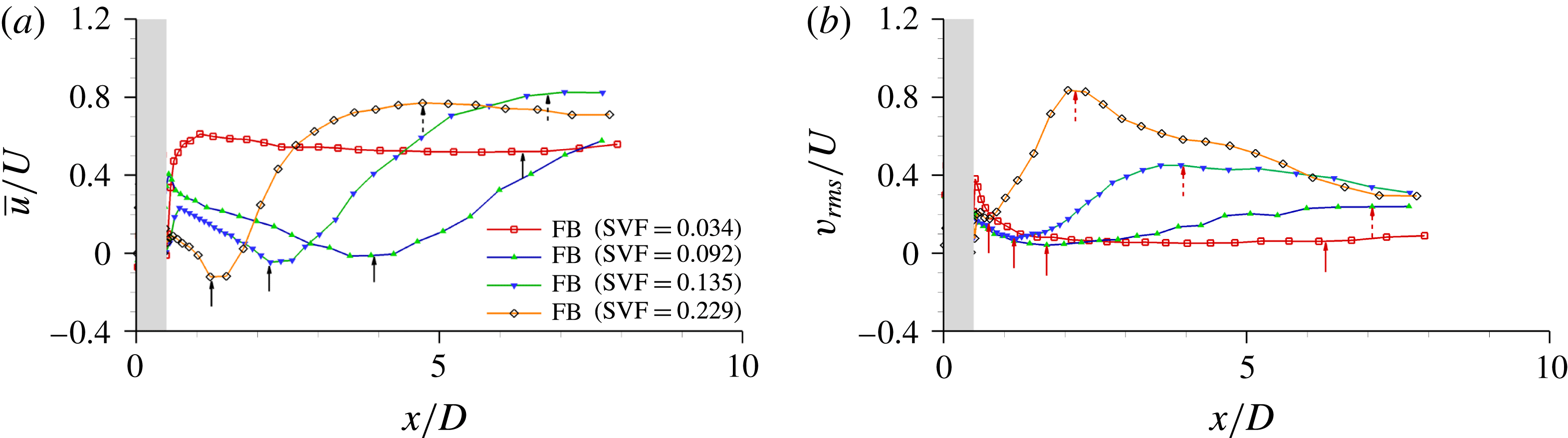
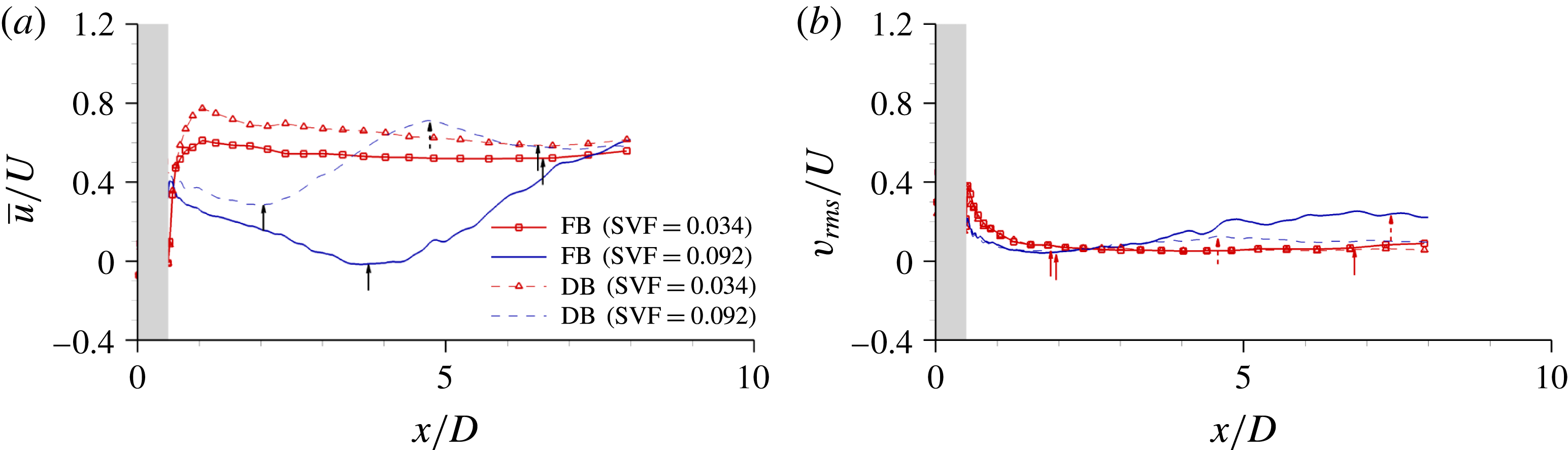
5 Spatial extent of the wake region

Following Zong & Nepf (Reference Zong and Nepf2012), the centreline profiles of the mean streamwise velocity, $\overline{u}/U$ , at the free surface are used to estimate the length of the steady wake region, $L_{1}$ , and the total length of the wake region, $L$ (figures 12 a and 13 a). The distance between the location where $\overline{u}/U$ reaches a minimum and the back of the porous cylinder ( $x/D=0.5$ ) is denoted $L_{1}$ . The length from the back of the cylinder to the location where the non-dimensional streamwise gradient of the mean streamwise velocity, $\unicode[STIX]{x2202}(\overline{u}/U)/\unicode[STIX]{x2202}(x/D)$ , becomes smaller than a threshold value (0.02) is denoted  $L$ . The length $L$ approximately corresponds to the distance from the porous cylinder to where wake billows form for cases where the antisymmetric shedding mode is present. The length of the steady wake region and the total length of the wake region are also estimated based on the centreline profiles of the r.m.s. of the lateral velocity near the free surface, $v_{rms}/U$ , shown in figures 12(b) and 13(b), following the procedure proposed by Chang & Constantinescu (Reference Chang and Constantinescu2015). The corresponding values of these lengths are denoted $L_{1}^{\prime \prime }$ and $L^{\prime \prime }$ respectively. The length $L_{1}^{\prime \prime }$ is defined as the distance from the back of the cylinder to the upstream end of the region where $v_{rms}$ starts to increase monotonically. The length $L^{\prime \prime }$ is defined as the distance from the back of the porous cylinder to the location of the peak of $v_{rms}/U$ , which is denoted $v_{rms,max}/U$ in table 1. If the antisymmetric mode is present, one expects that $v_{rms}$ will peak around the location where the wake billows form. Use of $L^{\prime \prime }$ to define the total length of the wake region eliminates the dependence on an arbitrary threshold value used to define  $L$ .

Figure 12.

Longitudinal profiles of (a) streamwise velocity, $\overline{u}/U$ , and (b) r.m.s. of the lateral velocity fluctuations, $v_{rms}/U$ , near the free surface ( $z/h=0.9$ ). The profiles are shown along the centreline, $y/D=0$ , for the flat-bed (FB) cases with $\text{SVF}=0.034$ , 0.092, 0.14 and 0.23. The grey region shows the extent of the porous cylinder ( $-0.5\leqslant x/D\leqslant 0.5$ ). The black solid arrows in (a) show the end of the steady wake region based on the length $L_{1}$ , the black dashed arrows in (a) show the end of the total wake region based on the length  $L$ , the red solid arrows in (b) show the end of the steady wake region based on the length $L_{1}^{\prime \prime }$ and the red dashed arrows in (b) show the end of the total wake region based on the length  $L^{\prime \prime }$ .

Figure 13.

Longitudinal profiles of (a) streamwise velocity, $\overline{u}/U$ , and (b) r.m.s. of the lateral velocity fluctuations, $v_{rms}/U$ , near the free surface ( $z/h=0.9$ ). The profiles are shown along the centreline, $y/D=0$ , for the flat-bed (FB) and deformed-bed (DB) cases with $\text{SVF}=0.034$ and 0.092. The grey region shows the extent of the porous cylinder ( $-0.5\leqslant x/D\leqslant 0.5$ ), the black solid arrows in (a) show the end of the steady wake region based on the length $L_{1}$ , the black dashed arrows in (a) show the end of the total wake region based on the length $L$ , the red solid arrows in (b) show the end of the steady wake region based on the length $L_{1}^{\prime \prime }$ and the red dashed arrows in (b) show the end of the total wake region based on the length  $L^{\prime \prime }$ .

In the flat-bed cases, increase in the SVF results in a decrease of the minimum streamwise velocity used to identify the end of the steady wake region (figure 12 a). The decrease of the minimum peak velocity with increasing SVF is fairly small for $\text{SVF}>0.1$ . The velocity at the start of the steady wake region, $U_{1}/U$ , is a relevant velocity scale for the present flow as it characterizes the strength of the bleeding flow at the back of the porous region (see also table 1). The profile of $\overline{u}/U$ has a relative maximum at this location, which is generally situated a short distance from the back of the porous cylinder. The results in figure 12(a) show that the streamwise velocity inside the steady wake region decreases by approximately $0.3U$ for $\text{SVF}>0.05$ . It is only for cases with very small SVFs that the centreline velocity inside the steady wake region is characterized by a small decay in the streamwise direction inside the steady wake region. The peak value of $v_{rms}/U$ along the centreline increases with increasing SVF (figure 12 b). A monotonic decrease of $L_{1}$ and $L$ with increasing SVF is observed for the flat-bed cases (figure 12 a). The same observation applies for $L_{1}^{\prime \prime }$ and $L^{\prime \prime }$ (figure 12 b).

The streamwise variations of $\overline{u}/U$ along the centreline are qualitatively similar in the $\text{SVF}=0.034$ cases with flat and deformed beds (figure 13 a). The main difference is the increase by approximately 20 % of $U_{1}/U$ as the bed evolves from flat to equilibrium scour conditions. The difference between the values of $\overline{u}/U$ at the start and end of the erosion and deposition process reduces significantly towards the end of the steady wake region. The distribution of $v_{rms}/U$ along the centeline varies little during the erosion and deposition process for this case (figure 13 b). Much larger differences are observed between the free-surface profiles of $\overline{u}/U$ in the $\text{SVF}=0.092$ case (figure 13 a), where the development of a deformed bed leads to significant weakening of the antisymmetric vortex shedding mode. Still, the overall shape of the $\overline{u}/U$ profile is similar in the flat-bed and equilibrium scour bed $\text{SVF}=0.092$ simulations. Although the velocity at the upstream end of the steady wake region is approximately the same in both simulations, the velocity at the downstream end of the steady wake region increases as the bed evolves towards equilibrium conditions. This increase is related to the reduction in the length of the steady wake region (e.g. $L_{1}$ decays from $3.5D$ to $1.5D$ in the $\text{SVF}=0.092$ case). For the $\text{SVF}=0.034$ case, for which the antisymmetric mode is absent even in flat-bed conditions, the development of the scour hole had a negligible effect on the value of $L_{1}$ (e.g. see figure 13 a and table 1 for the $\text{SVF}=0.034$ case). In the $\text{SVF}=0.092$ case, where the total wake length can be estimated based on the proposed definitions, a significant reduction in the values of $L$ and $L^{\prime \prime }$ is observed between flat-bed and equilibrium scour conditions (figure 13 and table 1).

Figure 14.

The main variables characterizing the near-wake region plotted as a function of the velocity ratio $U_{1}/U_{2}$ , the turbulence intensity $v_{rms,max}/U$ and the SVF: (a)  $L_{1}/D$ versus $U_{1}/U_{2}$ ; (b)  $L/D$ versus $U_{1}/U_{2}$ ; (c)  $L_{2}/D$ versus $v_{rms,max}/U$ ; (d)  $U_{1}/U$ versus SVF. The experimental data of Zong & Nepf (Reference Zong and Nepf2011) and Follett & Nepf (Reference Follett and Nepf2012) are included.

Figures 14(a) and 14(b) show the variation of $L_{1}/D$ and $L/D$ with the velocity ratio $U_{1}/U_{2}$ , where $U_{2}$ is the maximum velocity in the acceleration region forming on the outer side of the SSLs. The values of $L_{1}$ and $L$ predicted by the present simulations with flat and deformed beds are compared with those in the flat-bed experiments reported by Zong & Nepf (Reference Zong and Nepf2011) and the 3-D LES conducted for long porous cylinders by Chang & Constantinescu (Reference Chang and Constantinescu2015). Overall, the level of agreement with the values of $L_{1}$ and $L$ inferred from the experiments is good for the flat-bed cases. The values estimated for the deformed-bed cases are in fair agreement (e.g. within a 25 % difference) with those estimated for the flat-bed experiments for $U_{1}/U_{2}>0.2$ . The scatter in the experimental data is very high for low values of $U_{1}/U_{2}$ . A one-to-one comparison between the present cases and the long-cylinder cases cannot be made because, even for cases with the same SVF, the ratio $d/D$ and the relative distance between the cylinders in the array are not exactly the same in the two studies. Still, the ranges of values predicted for $L_{1}$ and $L$ in the present flat-bed simulations and the long-cylinder cases considered by Chang & Constantinescu (Reference Chang and Constantinescu2015) are in good agreement (e.g. see figure 14 a,b), which allows us to conclude that the length of the wake region near the free surface is approximately the same as the one for very deep cases, at least for moderately shallow cases.

Following Zong & Nepf (Reference Zong and Nepf2012), we also plot in figures 14(c) and 14(d) the variation of $L_{2}=L-L_{1}$ with the peak value of the spanwise velocity fluctuations, $v_{rms,max}$ , and that of the streamwise velocity at the upstream end of the steady wake region with the SVF. The agreement between the present flat-bed simulations and the flat-bed experiments of Zong & Nepf (Reference Zong and Nepf2011) is very satisfactory (less than 10 % difference between predicted values and those inferred via interpolation of the experimental values). The large reduction in the total wake length in the deformed-bed simulation with $\text{SVF}=0.092$ compared with the corresponding flat-bed case is the main reason why the point corresponding to this case falls away from the data corresponding to the flat-bed cases in figure 14(c). Related to the variation of $U_{1}/U$ with SVF in figure 14(d), a better agreement with the experimental results of Zong & Nepf (Reference Zong and Nepf2011) is observed for the present flat-bed simulations than that shown by the long-cylinder simulations of Chang & Constantinescu (Reference Chang and Constantinescu2015), especially for $\text{SVF}>0.1$ .

Figure 14(d) also includes results from the experiments of Follett & Nepf (Reference Follett and Nepf2012) conducted with a movable bed. The numerical predictions of the length of the steady wake region and $U_{1}/U$ at equilibrium scour conditions ( $L_{1}/D=6.0$ , $U_{1}/U=0.75$ for $\text{SVF}=0.034$ and $L_{1}/D=1.5$ , $U_{1}/U=0.1$ for $\text{SVF}=0.092$ ) are consistent with the values ( $L_{1}/D>5.5$ , $U_{1}/U=0.7$ for $\text{SVF}=0.034$ and $L_{1}/D=2.4$ , $U_{1}/U=0.08$ for $\text{SVF}=0.092$ ) inferred from the experiments of Follett & Nepf (Reference Follett and Nepf2012). This also explains the good agreement observed between the numerical simulations and the corresponding experiments conducted with a deformed bed in figure 14(d).

Figure 15.

The length of the steady wake region, $L_{1}/D$ , as a function of the non-dimensional flow blockage parameter, $\overline{C}_{d}^{\prime \prime }aD$ .

Following Chen et al. (Reference Chen, Ortiz, Zong and Nepf2012), the variation of the length of the steady wake region, $L_{1}/D$ , is plotted as a function of a non-dimensional blockage parameter, $\overline{C}_{d}^{\prime \prime }aD$ , in figure 15. To allow a direct comparison with the experimental data of Chen et al. (Reference Chen, Ortiz, Zong and Nepf2012), the drag coefficient $\overline{C}_{d}^{\prime \prime }$ is estimated based on the value of the Reynolds number defined with the solid cylinder diameter, $d$ , and the mean velocity inside the porous cylinder, $U_{p}$ , which is directly estimated from the numerical simulation. The values of $\overline{C}_{d}^{\prime \prime }$ are obtained using the procedure presented by Tanino & Nepf (Reference Tanino and Nepf2008). The agreement with the experimental data of Chen et al. (Reference Chen, Ortiz, Zong and Nepf2012) is very good for $\overline{C}_{d}^{\prime \prime }aD<10$ . The numerical simulations with no bed conducted by Chang & Constantinescu (Reference Chang and Constantinescu2015) and the present simulations with flat and deformed beds predict a fairly monotonic decay of $L_{1}/D$ for $\overline{C}_{d}^{\prime \prime }aD>10$ .

6 Bed friction velocity

To reveal the main mechanism for sediment entrainment inside and around porous cylinders, the effects of the SVF and $d/D$ on the bed friction velocity distribution are analysed next for some of the flat-bed cases. The extent of the steady wake region, the antisymmetric shedding of wake billows, the shedding of eddies in the wake of the solid cylinders and the formation of a necklace vortex around the upstream base of the cylinder have important consequences for the distribution of the bed friction velocity. For example, the passage of wake billows can induce a large amount of sediment entrainment behind the porous cylinder at locations where the mean value of the bed friction velocity is far beneath the mean critical value given by the Shields diagram or other methods used to estimate this variable (Miller, McCave & Komar Reference Miller, McCave and Komar1977). This statement is supported by the findings of Tinoco & Coco (Reference Tinoco and Coco2016) and Yang et al. (Reference Yang, Chung and Nepf2016) based on experimental observations of sediment entrainment and resuspension in such flows. The distribution of the bed friction velocity in the instantaneous flow field, $u_{\unicode[STIX]{x1D70F}}/U$ , allows investigation of the direct link between the presence, or the regular passage, of large-scale coherent structures over a certain bed location and the formation of regions of high/low $u_{\unicode[STIX]{x1D70F}}$ which would result in sediment entrainment from the bed. To characterize in an average way the capacity of the flow to entrain sediment, one has to consider not only the mean value of the bed friction velocity, $\overline{u}_{\unicode[STIX]{x1D70F}}$ , but also the temporal variation of the bed friction velocity with respect to the mean value. This is why we discuss not only the distribution of $\overline{u}_{\unicode[STIX]{x1D70F}}/U$ , but also that of the standard deviation of the bed friction velocity, $u_{\unicode[STIX]{x1D70F}}^{SD}/U$ , which serves to characterize in an approximate way the (larger-scale) temporal fluctuations of the bed friction velocity induced by the coherent structures present in the vicinity of the bed. Given that the first point off the wall is placed at less than two wall units, the bed friction velocity is calculated using the definition, without using wall functions. The magnitude of the local bed friction velocity in the instantaneous flow is defined as $u_{\unicode[STIX]{x1D70F}}/U=((1/Re)((u_{m}/U)/(n_{1}/H_{0})))^{1/2}$ , where $u_{m}$ is the instantaneous velocity magnitude in a plane parallel to the bed situated at a normal distance $n_{1}$ from the bed. The distance $n_{1}$ is sufficiently small for the plane to cut through the viscous sublayer. The same definition is used to calculate the bed friction velocity in the mean flow, with $u_{m}$ being the mean velocity magnitude in the same plane. When calculating the standard deviation of the bed friction velocity, $u_{m}$ is replaced by the square root of the turbulent kinetic energy in the same plane.

Figure 16.

The non-dimensional distribution of the mean bed friction velocity magnitude (a,b,g,h), the standard deviation of the bed friction velocity (c,d,i,j) and the instantaneous bed friction velocity magnitude (e,f,k,l) in the flat-bed cases with (a,c,e)  $\text{SVF}=0.034$ , (b,d,f)  $\text{SVF}=0.092$ , (g,i,k)  $\text{SVF}=0.23$ and (h,j,l)  $\text{SVF}=1.0$ .

At very low SVFs (e.g. $\text{SVF}=0.034$ in figure 16 a,c,e), the regions of high $\overline{u}_{\unicode[STIX]{x1D70F}}$ inside the porous region are situated on the sides of the solid cylinders, where the flow accelerates as it passes each cylinder. This mechanism for the amplification of $\overline{u}_{\unicode[STIX]{x1D70F}}$ is essentially the same as that for an isolated cylinder. Additionally, in the case of an array of cylinders, there is a certain level of amplification of $\overline{u}_{\unicode[STIX]{x1D70F}}$ due to the flow contraction as the bleeding flow is forced through the gap between neighbouring cylinders. The near wakes of the solid cylinders are characterized by low values of $\overline{u}_{\unicode[STIX]{x1D70F}}$ . Meanwhile, $u_{\unicode[STIX]{x1D70F}}^{SD}$ peaks in the same region, indicating that vortex shedding behind the solid cylinders may be an important mechanism for scour inside the porous cylinder. This is important, as for low SVFs, the coherence of the shed vortices is large and comparable to that observed past isolated cylinders for most of the cylinders in the array (see also figure 7 a). On the other hand, the amplification of $\overline{u}_{\unicode[STIX]{x1D70F}}$ and $u_{\unicode[STIX]{x1D70F}}^{SD}$ beneath the SSLs of the porous cylinder is fairly small (less than 50 % compared with the values observed on the channel bed at large distances upstream of the porous cylinder). Still, the distribution of the instantaneous bed shear stress shows that, at times, the levels of $u_{\unicode[STIX]{x1D70F}}$ in the upstream part of the SSLs are comparable to those observed on the sides of the solid cylinders inside the array. This is mainly because a relatively small percentage of the incoming flow approaching the porous cylinder is deflected laterally around it. As expected, the region situated in between the SSLs is characterized by small values of $u_{\unicode[STIX]{x1D70F}}$ and $\overline{u}_{\unicode[STIX]{x1D70F}}$ . The distributions of $\overline{u}_{\unicode[STIX]{x1D70F}}$ and $u_{\unicode[STIX]{x1D70F}}^{SD}$ are consistent with the scour patterns observed at equilibrium conditions (figure 2 a), where the most severe scour occurs inside the porous region, virtually no scour develops around the upstream base of the porous cylinder and the scour on the sides of the porous cylinder is fairly small compared with that observed inside the porous region. Most of the sediment deposition occurs in a region ( $0.6<x/D<1.4$ ) characterized by very small values of $\overline{u}_{\unicode[STIX]{x1D70F}}$ and $u_{\unicode[STIX]{x1D70F}}^{SD}$ . Still, one should be careful about trying to predict scour patterns in the later stages of the erosion and deposition process based on the bed friction velocity distributions during the initial stages of the erosion process. For example, the distributions of $u_{\unicode[STIX]{x1D70F}}$ in figure 16(a,c,e) do not give any indication why a V-shaped ridge of deposited sediment forms for $x/D>1.4$ (figure 2 a).

As the SVF increases and antisymmetric vortex shedding is observed in the wake of the porous cylinder, several important qualitative changes occur in the bed friction velocity distributions (e.g. compare figures 16 a,c,e and 16 b,d,f for $\text{SVF}=0.034$ and 0.092 respectively). Due to the larger adverse pressure gradients in the $\text{SVF}=0.092$ case, a larger part of the incoming flow approaching the porous cylinder is deflected laterally, which results in a very large amplification of $\overline{u}_{\unicode[STIX]{x1D70F}}$ and $u_{\unicode[STIX]{x1D70F}}$ on the sides of the porous cylinder and the outer side of the SSLs (figure 16 b,d,f). This region of flow acceleration has a maximum width of approximately $1D$ and extends until the end of the steady wake region. At the same time, ‘corridors’ of relatively high $\overline{u}_{\unicode[STIX]{x1D70F}}$ form inside the upstream part of the porous region in the $\text{SVF}=0.092$ case, as the relatively high-velocity fluid penetrating inside the porous region locally accelerates as it passes in between two rows of solid cylinders (figure 16 b,d,f). These ‘corridors’ are oriented along the streamwise direction only at small lateral distances from the symmetry plane ( $y/D=0$ ) and start to make an angle with the streamwise direction at larger $y/D$ . The orientation of the ‘corridors’ is consistent with the observed mean flow pattern inside the porous region, away from the bed surface (figure 10 b). Due to the drag induced by the solid cylinders on the bleeding flow, the fluid advected inside these ‘corridors’ gradually decelerates. This explains the decay of $\overline{u}_{\unicode[STIX]{x1D70F}}$ and $u_{\unicode[STIX]{x1D70F}}$ for $x/D>0.3$ . As opposed to the $\text{SVF}=0.032$ case, where the regions of high $u_{\unicode[STIX]{x1D70F}}^{SD}$ correspond to the wakes of the solid cylinders, in the $\text{SVF}=0.092$ case, $u_{\unicode[STIX]{x1D70F}}^{SD}$ is amplified over most of the porous region in between $x/D=-0.3$ and $x/D=0.3$ . Only over the upstream part of the porous region ( $x/D<-0.3$ ) do regions of high $u_{\unicode[STIX]{x1D70F}}^{SD}$ correspond to the wakes of the solid cylinders directly or partially exposed to the incoming flow. The reason for the large amplification of $u_{\unicode[STIX]{x1D70F}}^{SD}$ for $-0.3<x/D<0.3$ is the strong wake-to-cylinder and wake-to-wake interactions, which result in entrainment of billows shed from the wakes of the solid cylinders into the higher-speed flow inside the ‘corridors’. The region where most of the scour inside the porous cylinder occurs at equilibrium conditions (figure 2 b) is approximately the same as the region ( $x/D<0.3$ ) where high values of $\overline{u}_{\unicode[STIX]{x1D70F}}$ and $u_{\unicode[STIX]{x1D70F}}^{SD}$ are observed at the start of the scour and deposition process.

Given the much weaker bleeding flow entering the region between the SSLs at the back of the porous cylinder in the $\text{SVF}=0.092$ case compared with the $\text{SVF}=0.034$ case, the values of $\overline{u}_{\unicode[STIX]{x1D70F}}$ are very small inside the steady wake region in the $\text{SVF}=0.092$ case. As expected, the formation of the wake billows results in a fairly large amplification of $u_{\unicode[STIX]{x1D70F}}$ beneath the newly formed billow (e.g. a billow is present at $x/D\approx 6.5$ in the $u_{\unicode[STIX]{x1D70F}}$ field shown in figure 16 b,d,f). However, these billows are not very coherent compared with those observed at very high SVFs, and the $u_{\unicode[STIX]{x1D70F}}$ values at the same locations are very low once the billow has left the region. Thus, the values of $\overline{u}_{\unicode[STIX]{x1D70F}}$ are quite low in this region. Still, these billows can entrain and carry sediment downstream of the steady wake.

At relatively high SVF values ( $\text{SVF}>0.2$ ), most of the incoming flow is diverted laterally, similarly to the case of a solid cylinder. For example, in the $\text{SVF}=0.23$ case, the main region of high $\overline{u}_{\unicode[STIX]{x1D70F}}$ is situated on the outer side of the porous cylinder and extends on the outer side of its SSLs until the end of the steady wake region. Within this flow acceleration region, the size of the region with $\overline{u}_{\unicode[STIX]{x1D70F}}/U>0.05$ is by more than 50 % higher in the $\text{SVF}=0.23$ case (figure 16 g,i,k) compared with the $\text{SVF}=0.092$ case (figure 16 b,d,f). The same is true for the peak values of $\overline{u}_{\unicode[STIX]{x1D70F}}$ within this flow acceleration region. Meanwhile, the ‘corridors’ of high $\overline{u}_{\unicode[STIX]{x1D70F}}$ penetrate only until $x/D\approx 0$ in the $\text{SVF}=0.23$ case. The region of high $u_{\unicode[STIX]{x1D70F}}^{SD}$ inside the porous cylinder also extends only until $x/D=0$ . On the other hand, the level of amplification of $\overline{u}_{\unicode[STIX]{x1D70F}}$ and $u_{\unicode[STIX]{x1D70F}}^{SD}$ inside the SSLs of the porous cylinder is much higher in the $\text{SVF}=0.23$ case, which is expected given the large acceleration of the flow velocity as it passes the porous cylinder and the larger coherence of the eddies advected inside the SSL in the $\text{SVF}=0.23$ case compared with the $\text{SVF}=0.092$ case. The level of amplification of $\overline{u}_{\unicode[STIX]{x1D70F}}$ and $u_{\unicode[STIX]{x1D70F}}^{SD}$ inside the SSLs continues to increase with increasing SVF (e.g. compare the distributions for the $\text{SVF}=0.23$ case and the $\text{SVF}=1.0$ case in figure 16). Therefore, for $\text{SVF}>0.2$ , one expects that most of the scour will initially develop on the sides of the porous cylinder and beneath the SSLs, similarly to what is observed for solid cylinders mounted on a loose bed.

The small region of relatively high $u_{\unicode[STIX]{x1D70F}}^{SD}$ observed close to the upstream base of the porous cylinder in the $\text{SVF}=0.23$ case is due to the presence of a necklace vortex (figure 4 e). Its coherence is not very high, which explains why the values of $\overline{u}_{\unicode[STIX]{x1D70F}}$ over the same region are only slightly larger than those observed in the approaching flow. As the SVF is further increased, the necklace vortex becomes more coherent and its core is subject to bimodal oscillations. Figure 16(h,j,l) shows results for the limiting case of a solid cylinder ( $\text{SVF}=1$ ). The region of high $\overline{u}_{\unicode[STIX]{x1D70F}}$ in front of the solid cylinder penetrates until the symmetry plane, while large values of $u_{\unicode[STIX]{x1D70F}}^{SD}$ are observed at all locations beneath the core of the main necklace vortex.

Large differences are also observed in the distribution of the bed friction velocity in the wake of the porous cylinder among the $\text{SVF}=0.092$ (figure 16 b,d,f), $\text{SVF}=0.23$ (figure 16 g,i,k) and $\text{SVF}=1.0$ (figure 16 h,j,l) cases. For $\text{SVF}>0.2$ , the highest values of $u_{\unicode[STIX]{x1D70F}}^{SD}$ are not observed inside the porous region any more, but rather in the region where the ends of the SSLs bend towards each other and wake billows form ( $1.5<x/D<2.5$ for $\text{SVF}=0.23$ ). The coherence of the wake billows in their formation region increases with increasing SVF. So does their capacity to induce large bed friction velocities, as observed by comparing the distributions of $u_{\unicode[STIX]{x1D70F}}$ in figures 16(b,d,f), 16(g,i,k) and 16(h,j,l). Moreover, for $\text{SVF}>0.2$ , the capacity of the wake billows to induce large bed friction velocities remains high after they start moving away from the formation region.

Figure 17.

The mean non-dimensional force, $\overline{\boldsymbol{F}}^{n}/(0.5\unicode[STIX]{x1D70C}U^{2}\,\text{d}h)=\overline{C}_{D}^{n}\boldsymbol{i}\pm \overline{C}_{DL}^{n}\,\boldsymbol{j}$ , acting on the solid cylinders within the array: (a)  $\text{SVF}=0.034$ ; (b)  $\text{SVF}=0.034$ , deformed bed; (c)  $\text{SVF}=0.092$ ; (d)  $SVF=0.23$ . The black vector at the top right corner corresponds to the mean (streamwise) non-dimensional force predicted on an isolated solid cylinder of diameter $d=0.03D$ .

7 Drag forces

Figure 17 compares the time-averaged non-dimensional force vector acting on the solid cylinders within the array, $\overline{\boldsymbol{F}}^{n}/(0.5\unicode[STIX]{x1D70C}U^{2}\,\text{d}h)=\overline{C}_{D}^{n}\boldsymbol{i}\pm \overline{C}_{L}^{n}\,\boldsymbol{j}$ , for several representative cases with flat and deformed beds, where $n$ is the index of the solid cylinder, and $\overline{C}_{D}^{n}=\overline{F}_{x}^{n}/(0.5\unicode[STIX]{x1D70C}U^{2}\,\text{d}h^{n})$ and $\overline{C}_{DL}^{n}=\overline{F}_{y}^{n}/(0.5\unicode[STIX]{x1D70C}U^{2}\,\text{d}h^{n})$ are the streamwise and lateral ( $y$ -direction) drag forces acting on the solid cylinder of height $h^{n}$ . For the flat-bed cases, $h^{n}=h$ .

On average, the force acting on the solid cylinders directly exposed to the incoming flow decreases with increasing SVF (see figures 17 a, 17 c,d comparing the flat-bed cases). Because of the adverse pressure gradients associated with the porous cylinder region, the mean force acting on the cylinders directly exposed to the incoming flow situated close to the symmetry plane is smaller than that observed for an isolated solid cylinder of the same diameter, $d$ . The difference is only of the order of 10 % for the $\text{SVF}=0.034$ case and increases to approximately 65 % for the $\text{SVF}=0.23$ case. The peak forces are observed for cylinders situated close to the upstream face of the porous region at polar angles of approximately $35^{\circ }{-}90^{\circ }$ in the larger-SVF cases (figure 17 c,d). This is the region where the maximum flow acceleration occurs in the immediate vicinity of the porous cylinder. For some of these solid cylinders, the magnitude of the drag force is slightly larger than that observed for an isolated cylinder. At small SVFs, the drag forces on all cylinders in the arrays have a fairly negligible component along the lateral direction (e.g. case $\text{SVF}=0.034$ in figure 17 a). As the SVF increases, the drag forces on the solid cylinders acquire an important lateral component in the $x/D<0$ region (e.g. see figure 17 d), consistent with the bleeding flow pattern inside the porous region (figure 10 c).

In all cases, the drag force decreases, on average, with increasing distance from the upstream edge of the porous region. For relatively low SVFs, where the flow is in what can be called the low-flow-blockage regime (e.g. $\text{SVF}<0.09$ ), the rate of decrease of the average drag force acting on the individual cylinders increases with increasing SVF (e.g. compare the forces acting on the cylinders in figure 17 a,c). Once the flow inside the porous patch can be considered to transition to the high-flow-blockage regime ( $\text{SVF}>0.09$ ), the reduction in drag force between cylinders situated close to the leading and trailing edges of the porous patch is fairly independent of the SVF, as the momentum decay scale is the diameter of the porous cylinder, which is the same in the present test cases. With the exception of a couple of cylinders shielded by the wake of the upstream cylinders, the drag forces acting on the cylinders situated close to the downstream face of the porous cylinder in the $\text{SVF}=0.034$ case are larger than 50 % of the average force acting on the cylinders directly exposed to the incoming flow. In the $\text{SVF}=0.092$ case, the drag forces acting on most of the solid cylinders situated in the $x/D>0.1$ region are less than 50 % of the average force acting on the cylinders directly exposed to the incoming flow. For the $\text{SVF}=0.23$ case, the same is true for most of the cylinders situated in the $x/D>-0.15$ region. The randomness of the orientation of the drag forces on the solid cylinders also increases with the SVF (e.g. compare the $\text{SVF}=0.092$ and $\text{SVF}=0.23$ cases in figure 17) because of the increase of the wake-to-cylinder interactions as the distance among the cylinders in the arrays decreases. Comparison of the distributions of the drag forces in the $\text{SVF}=0.034$ cases with flat (figure 17 a) and deformed (figure 17 b) beds reveals that the magnitude of the drag force slightly decreases as the bed evolves towards equilibrium.

Analysis of the forces acting on the individual cylinders shows that the distribution of the forces is strongly dependent on the SVF. In the $\text{SVF}=0.034$ case (figure 17 a), around 85 % of the cylinders in the array are subject to forces that are larger than 50 % of the force acting on an isolated cylinder, with virtually no cylinder being subject to forces that are less than 25 % of the force acting on an isolated cylinder. In contrast, in the $\text{SVF}=0.23$ case (figure 17 d), around 70 % of the cylinders in the array are subject to forces that are less than 25 % of the force acting on an isolated cylinder, and only 12 % of them are subject to forces that are larger than 50 % of the force acting on an isolated cylinder. On the other hand, in the $\text{SVF}=0.092$ case, most of the cylinders in the arrays are subject to forces of between 25 % and 50 % of the force acting on an isolated cylinder (figure 17 c).

Figure 18.

The non-dimensional time-averaged streamwise drag force. (a) Time-averaged total drag coefficient for the array, $\overline{C}_{DG}$ , versus SVF; (b) mean time-averaged solid cylinder drag coefficient, $\overline{C}_{d}=(\overline{C}_{DG}/N)(D/d)$ , versus SVF; (c)  $\overline{C}_{d}$ versus $aD$ in linear–linear scale; (d)  $\overline{C}_{d}$ versus $aD$ in log–linear scale; (e) non-dimensional flow blockage parameter $\overline{C}_{d}^{\prime }aD$ versus SVF in linear–linear scale; (f) combined drag parameter for the porous cylinder, $\unicode[STIX]{x1D6E4}_{D}=\overline{C}_{d}(aD)/(1-\text{SVF})$ , versus $aD$ . Besides the present test cases with flat and deformed beds, results are also included from the 2-D DNS of Nicolle & Eames (Reference Nicolle and Eames2011) and the 3-D LES of Chang & Constantinescu (Reference Chang and Constantinescu2015) conducted for long porous cylinders (no bed). The red line in (d) shows a best fit to the numerical data. Also included in (e) are the experimental data of Tinoco & Cowen (Reference Tinoco and Cowen2013) for arrays of rigid cylinders. The dashed line in (e) shows the best fit to the experimental data ( $\overline{C}_{d}^{\prime }aD=16.53\,\text{SVF}^{2}+1.47\text{SVF}$ ) proposed by Tinoco & Cowen (Reference Tinoco and Cowen2013).

The time-averaged non-dimensional forces acting on the porous cylinder are discussed next. The mean force acting on the porous cylinder is $\overline{\boldsymbol{F}}=\sum _{n=1}^{N}\overline{\boldsymbol{F}}^{n}$ . Using the streamwise component, one can define a total drag coefficient, $\overline{C}_{DG}=\overline{F}_{x}/(0.5\unicode[STIX]{x1D70C}U^{2}Dh)$ , and an average drag coefficient for the solid cylinders in the array, $\overline{C}_{d}=(\overline{C}_{DG}/N)(D/d)=(1/N)\sum _{n=1}^{N}\overline{C}_{D}^{n}$ . These two drag coefficients are plotted in figure 18(a,b) as a function of the SVF for the flat-bed and deformed-bed cases. Also included are the drag coefficients evaluated from the 2-D DNS of Nicolle & Eames (Reference Nicolle and Eames2011) and the 3-D LES of Chang & Constantinescu (Reference Chang and Constantinescu2015) conducted for long cylinders. The flat-bed results are fairly close to the corresponding long-cylinder simulations. For both types of simulations, an increase of $d/D$ results in a relatively large decrease of $\overline{C}_{DG}$ and an increase of $\overline{C}_{d}$ . For constant $d/D$ , $\overline{C}_{d}$ decreases monotonically with increasing SVF. The values of $\overline{C}_{DG}$ and $\overline{C}_{d}$ at equilibrium bed conditions are approximately 10 %–15 % lower than those estimated for the corresponding flat-bed cases. We also calculated $\overline{C}_{d}$ from the deformed-bed simulations using the drag forces acting only between the $z=h/2$ level and the free surface. An increase of 7 %–10 % of $\overline{C}_{d}$ was observed compared with the values estimated over the whole flow depth.

A plot of $\overline{C}_{d}$ as a function of $aD$ (figure 18 c) has the advantage that it basically eliminates the dependence of $\overline{C}_{d}$ on $d/D$ . The data from the four series of simulations collapse fairly well on a single curve. In particular, the $\overline{C}_{d}$ values predicted by the flat-bed simulations and the 3-D long-cylinder simulations are very close for similar values of $aD$ . Moreover, to a good approximation, the variation of $\overline{C}_{d}$ with $aD$ is logarithmic, at least for $0.1<aD<10$ (see figure 18 d, where the same data are plotted in a log–linear scale). The best fit equation is $\overline{C}_{d}=0.872{-}0.708\log (aD)$ .

A more general way to represent the dependence of the mean drag cylinder coefficient for an array of cylinders as a function of the characteristics of the array is to plot the non-dimensional flow blockage parameter as a function of the SVF. As mentioned by Tinoco & Cowen (Reference Tinoco and Cowen2013), the advantage of using the flow blockage parameter, $\overline{C}_{d}^{\prime }aD$ , is that it accounts for porous region properties other than the cylinder diameter, $d$ . The flow blockage parameter was defined by Tinoco & Cowen (Reference Tinoco and Cowen2013) using a mean cylinder drag coefficient, $\overline{C}_{d}^{\prime }$ , calculated using the mean velocity within the porous region, $U_{p}$ , as the velocity scale. The estimated values of $\overline{C}_{d}^{\prime }$ based on our numerical simulations are also included in table 1. Tinoco & Cowen (Reference Tinoco and Cowen2013) also proposed a simple polynomial variation for $\overline{C}_{d}^{\prime }aD$ with the SVF based on their experiments conducted with $\text{SVF}<0.1$ . One can see from figure 18(e) that the $\overline{C}_{d}^{\prime }aD$ values predicted by the present numerical simulations with flat and deformed beds are in very good agreement with the experimental values for $\text{SVF}<0.1$ and that the best fit proposed by Tinoco & Cowen (Reference Tinoco and Cowen2013) does a fairly good job in predicting $\overline{C}_{d}^{\prime }aD$ at larger SVF values.

For high-Reynolds-number cases, the dominant terms in the momentum balance within the porous region are the streamwise advection term $(1-\text{SVF})u(\unicode[STIX]{x2202}u/\unicode[STIX]{x2202}x)$ and the quadratic velocity drag term $\overline{C}_{d}au|u|$ , where $u$ is the local streamwise velocity. As discussed by Chang & Constantinescu (Reference Chang and Constantinescu2015), the ratio between these two terms characterizes the relative influence of the drag term relative to the advection term. This ratio defines a combined drag parameter for the porous medium, $\unicode[STIX]{x1D6E4}_{D}=\overline{C}_{d}aD/(1-\text{SVF})$ , where we assume that $\unicode[STIX]{x2202}u/\unicode[STIX]{x2202}x$ is of the order of the mean deceleration of the streamwise velocity across the porous cylinder, which scales with $U/D$ . The same parameter $\unicode[STIX]{x1D6E4}_{D}$ represents the ratio of the porous cylinder diameter, $D$ , to the canopy drag length scale, $L_{c}=2(1-\text{SVF})/(\overline{C}_{d}\cdot a)$ , proposed by Belcher, Jerram & Hunt (Reference Belcher, Jerram and Hunt2003). The range of $\unicode[STIX]{x1D6E4}_{D}$ in the present simulations is 0.83–2.44, which is fairly close to the range ( $0.68<\unicode[STIX]{x1D6E4}_{D}<2.57$ ) in the study of Chang & Constantinescu (Reference Chang and Constantinescu2015). The results in figure 18(f) show that $\unicode[STIX]{x1D6E4}_{D}$ increases fairly monotonically with $aD$ for $aD<8$ . Over this range of $aD$ , the differences between the predicted values of $\unicode[STIX]{x1D6E4}_{D}$ for the flat-bed and the long-cylinder simulations are small. For larger $aD$ values, $\unicode[STIX]{x1D6E4}_{D}$ starts to decrease. This is simply because the drag forces on the cylinders situated close to the back of the porous cylinder are negligible in the simulations with high SVF or $aD$ (e.g. this happens in the region with $z/D>0.25$ for the case with $\text{SVF}=0.23$ and $aD=9.6$ ). If one were to use the ‘active’ number of cylinders in the array to calculate $\overline{C}_{d}$ , then $\unicode[STIX]{x1D6E4}_{D}$ would be expected to continue to increase monotonically with $aD$ . A decrease of 10 %–15 % is observed for $\unicode[STIX]{x1D6E4}_{D}$ as the bed surface changes from flat to equilibrium bed conditions. This means that the bleeding flow will be relatively stronger as the bathymetry approaches equilibrium. As a result, the capacity of the flow to induce sediment resuspension inside an array of a given SVF will be enhanced as the bathymetry evolves towards equilibrium.

8 Summary and conclusions

Simulations conducted for a porous cylinder containing emerged solid circular cylinders placed in an open channel were used to investigate the flow structure, the sediment erosion mechanisms and the distribution of drag forces on the cylinders forming the array for moderately shallow conditions ( $h/D\approx 0.5$ ). The lateral deflection of part of the incoming flow around the upstream face of the porous cylinder generated a region of high bed friction velocities. For sufficiently large SVFs, scour around the porous cylinder would be initiated in this region. The size of this region and the peak values of the bed friction velocity within this region increase monotonically with the SVF. For $\text{SVF}>0.2$ , a necklace vortex forms close to the junction between the upstream face of the porous cylinder and the bed, as the downflow reaches the bed surface and moves away from the junction line. The size and coherence of the necklace vortex increase as the bed evolves towards equilibrium scour conditions and the SVF becomes larger. The necklace vortex increases the magnitude of the mean bed friction velocity and the r.m.s. of the bed friction velocity fluctuations beneath its core. At lower SVFs (e.g. for $\text{SVF}=0.14$ ), for which no necklace vortices developed around the porous cylinder, strong necklace vortices formed around the solid cylinders directly exposed to the incoming flow. Moreover, a large amplification of the turbulence was observed in front of the porous cylinder, in the near-bed region, even at SVF values that were lower than the minimum value required for a necklace vortex to form around the porous cylinder. This explains the presence of relatively large mean fluctuations of the bed friction velocity in front of the porous cylinder even in the absence of a necklace vortex.

As opposed to the case of a solid cylinder, where the downflow moves parallel to the face of the cylinder, in the case of a porous cylinder, part of the downflow penetrates inside the porous region and induces significant negative vertical velocities in the near-bed region inside the ‘corridors’ of higher-speed bleeding flow. Consistent with continuity, regions of strong upwelling are observed in the wakes of the solid cylinders, even in the simulations with a flat bed. The strength of these vertical motions decreases with increasing SVF for the flat-bed cases. The presence of a deformed bed induces an even larger secondary flow inside the deeper parts of the porous cylinder regions. The mean flow vertical motions together with the highly energetic eddies shed from the solid cylinders have a great effect on transport within the porous region. They also affect the deposition of fine particles and sediment retention within the porous region in cases where the flow transports sediments.

While, for $\text{SVF}<0.05$ , the region of high TKE extended over most the porous cylinder, for larger SVFs, this region occupied only the upstream part of the porous cylinder. For $\text{SVF}>0.2$ , the wake-to-cylinder interactions were very strong and the region of high TKE occupied only a narrow strip inside the upstream half of the porous cylinder. All of these changes mean that the dynamics of the suspended sediment and the transport of particulates entering the porous region will be very different for arrays of rigid cylinders with low and high SVFs. While, for $\text{SVF}<0.05$ , the main reason for the amplification of the bed friction velocity inside the porous cylinder was the flow acceleration on the sides of the solid cylinders and the shedding of billow vortices in their wakes, at higher SVFs ( $0.05<\text{SVF}<0.2$ ), most of the larger-scale eddies shed in the wakes of the solid cylinders were drawn into the ‘corridors’ of strong bleeding flow. Most of the amplification of the mean bed friction velocity occurs inside these ‘corridors’, while regions of high r.m.s. of the bed friction fluctuations approximately correspond to regions of high TKE at larger distances from the bed. These results suggest that scour inside the porous region increases with the SVF, in agreement with the observations of Follett & Nepf (Reference Follett and Nepf2012), whose experiments were conducted with $\text{SVF}<0.1$ . However, the present results show that for $\text{SVF}>0.2$ , the bleeding flow is quite week and the small distance between the solid cylinders suppresses the generation of large-scale energetic eddies in the wakes of these cylinders. Thus, scour inside the porous cylinder is expected to start to decrease past a certain threshold value of the SVF. Given the large capacity of the large-scale eddies shed in the wake of the solid cylinders to amplify the instantaneous bed shear stress, both variables should be used to assess the erosive capacity of the flow inside the porous region. In the flat-bed simulations, regions of high bed friction velocity inside the porous region and around its upstream base matched fairly well the regions where scour developed in the corresponding movable bed experiments.

At sufficiently high SVFs where the antisymmetric vortex shedding mode is observed, the coherence of the billows shed in the wake of the porous cylinder was found to increase monotonically with the SVF. For the flat-bed case, the reduction of the lengths of the steady wake and total wake regions with increasing SVF was close to that predicted for long cylinders by Chang & Constantinescu (Reference Chang and Constantinescu2015). Even for relatively low SVFs, the billow vortices were shown to have a large capacity to induce large bed friction velocities in the instantaneous flow fields in their formation region. As the bed evolved from flat to equilibrium scour conditions, the lengths of the steady wake and total wake regions decreased by up to 50 % for the two cases where simulations were conducted with both a flat bed and an equilibrium scour bed. For the $\text{SVF}=0.092$ case, where the antisymmetric shedding mode was strong in the flat-bed simulation, the development of the scour hole led to near suppression of the antisymmetric shedding mode. This result is not surprising, given that for similar moderately shallow conditions, Kirkil et al. (Reference Kirkil, Constantinescu and Ettema2009) observed experimentally and numerically that the antisymmetric shedding mode is totally supressed for solid cylinders in equilibrium scour conditions. This was due to the development of upwelling close to the symmetry plane at the back of the cylinder. The upwelled flow was deflected by the free surface and pushed away the SSLs on the two sides of the cylinder.

One of the main advantages of the present study is that it allowed estimation of the drag forces on the individual cylinders in the array and the mean time-averaged streamwise drag coefficient of the solid cylinders, $\overline{C}_{d}$ , for both flat-bed and deformed-bed cases. For the flat-bed cases, the distributions of the drag forces and their magnitudes were found to be a strong function of the SVF. While, for $\text{SVF}<0.05$ , more than 50 % of the cylinders in the array were subject to drag forces that were larger than 75 % of the maximum drag force in the array or the drag force acting on an isolated solid cylinder, for $\text{SVF}>0.2$ , more than 50 % of the cylinders in the array were subject to forces that were smaller than 25 % of the maximum drag force in the array, with close to negligible forces acting on approximately half of these cylinders. The present data show that, at least for the range of SVF and $aD$ values considered in the present study, the decay of $\overline{C}_{d}$ with $aD$ is logarithmic. This mean drag coefficient for the array is the main empirical parameter to be provided in less complex RANS and LES models which account for the presence of the solid cylinders by simply adding a quadratic drag term proportional to $\overline{C}_{d}$ when solving the momentum equations inside the porous region. Although the present results suggest that the use of a constant value of $\overline{C}_{d}$ in movable bed solvers that try to predict the evolution of scour inside and around the array of rigid cylinders is an acceptable approximation, a slight reduction of $\overline{C}_{d}$ with the development of the scour hole may be considered in solvers that do not resolve the flow past the individual cylinders in the array.

The present study investigated only the case of flow past an emerged array of rigid cylinders under moderately shallow conditions. It will be of great interest to investigate how the flow structure and sediment erosion mechanisms change with increasing submergence of the porous region (array of rigid cylinders), and how the wake structure changes with the main geometrical parameters defining the porous region as the ratio $D/h$ becomes much larger than one and flow shallowness effects are sufficiently large to suppress the antisymmetric shedding even if the porous cylinder is placed on a flat bed (Sukhodolov & Sukhodolova Reference Sukhodolov and Sukhodolova2014).