1. Introduction
Skin-friction drag in wall-bounded turbulence significantly surpasses its laminar counterpart at equivalent Reynolds numbers (Kim Reference Kim2011). In particular, it constitutes up to 50 % of the total drag on commercial aircraft, nearly 90 % for submarines and almost all drag for internal flows, such as those in pipe and channels. Therefore, understanding the physical mechanisms responsible for turbulent skin-friction generation and developing effective drag control strategies are of central importance for energy efficiency and environmental sustainability (Gad-el Hak Reference Gad-el Hak2007).
Although turbulent skin friction is inherently a wall property, defined based on the wall-normal gradient of the streamwise velocity, it is intimately connected with unsteady flow physics across the entire wall layers. The unsteady flow structures within the wall layer cause significant changes to the velocity field compared with laminar flows, leading to increased instantaneous and mean skin frictions. Over the past decades, a variety of decomposition frameworks have been proposed to relate the mean skin-friction coefficient to statistical flow quantities. For example, the seminal contribution of Fukagata, Iwamoto & Kasagi (Reference Fukagata, Iwamoto and Kasagi2002), widely known as the FIK identity, relates the mean skin-friction coefficient to the Reynolds shear-stress distribution in wall-bounded turbulence. An alternative viewpoint was later provided by Renard & Deck (Reference Renard and Deck2016), which interprets skin friction as the rate at which energy is transferred from the wall to the fluid through viscous dissipation and turbulence production. Building on these two pioneering identities, numerous extensions have recently been developed (Yoon et al. Reference Yoon, Ahn, Hwang and Sung2016; de Giovanetti et al. Reference de Giovanetti, Hwang and Choi2016; Chen et al. Reference Chen, Yao and Hussain2021), significantly advancing our understanding of skin-friction generation and drag-reduction mechanisms in wall-bounded flows (Elnahhas & Johnson Reference Elnahhas and Johnson2022; Ricco & Skote Reference Ricco and Skote2022; Floryan Reference Floryan2023; Zhao, Fan & Li Reference Zhao, Fan and Li2024).
Despite the progress enabled by existing decomposition frameworks, they focus primarily on mean or statistical quantities and therefore cannot identify the corresponding flow structures that are directly responsible for the turbulent skin-friction generation. It is well established that the skin-friction drag in wall turbulence arises predominantly from the near-wall self-sustaining cycle, namely, the regeneration of streamwise streaks and vortices. Therefore, most drag-reduction strategies aim to weaken or disrupt these quasi-coherent motions (Gatti & Quadrio Reference Gatti and Quadrio2016; Rastegari & Akhavan Reference Rastegari and Akhavan2018). At high Reynolds numbers, however, recent studies have demonstrated that large-scale and very-large-scale outer motions play an increasingly important role in contributing to the wall-shear stress (Marusic et al. Reference Marusic, Chandran, Rouhi, Fu, Wine, Holloway, Chung and Smits2021), suggesting that skin-friction generation results from a multiscale structural organisation spanning the entire wall layer. To probe the structural sources of the skin-friction generation, prior efforts have largely relied on correlation-based analyses or conditional averaging techniques (Jeong et al. Reference Jeong, Hussain, Schoppa and Kim1997; Hwang Reference Hwang2015). Despite important insights revealed by these methods, the connection between such flow structures and skin friction remains largely qualitative. This underscores the need for a unified framework that can quantitatively relate coherent flow structures to skin-friction generation, with which a more mechanistic understanding may be obtained, while consistent effectiveness comparisons among different control strategies may be made (Yao, Chen & Hussain Reference Yao, Chen and Hussain2018).
To achieve this goal, modal decomposition techniques may be used. Common decomposition techniques, such as proper orthogonal decomposition (POD) and dynamic mode decomposition (DMD), are widely used to extract coherent structures from complex turbulent flows. The resulting POD modes are ranked by their kinetic energy content, while DMD modes are ordered in terms of their `contribution’ to the overall dynamics of the underlying system. However, our interests are not to seek energetic or dynamically dominant structures, but rather those that contribute most directly to skin-friction generation. Because neither POD nor DMD is designed to target wall-shear stress, a large number of modes is typically required to reconstruct the instantaneous skin friction with reasonable accuracy. Recently, canonical correlation decomposition (CCD) (Lyu Reference Lyu2024a , Reference Lyub ) has been proposed as an observable, targeted decomposition technique that isolates flow structures most strongly correlated with a given quantity of interest, while suppressing uncorrelated contributions. This property makes CCD particularly well suited for identifying structures directly responsible for skin-friction generation. The main objective of the present work is to apply CCD to turbulent channel flows to extract and characterise these structures.
The paper is structured as follows. Section 2 outlines the CCD methodology and describes the direct numerical simulation (DNS) databases of turbulent channel flows used in this paper. Section 3 shows the resulting flow structures that are most strongly correlated with skin friction. The analysis is then extended to channel flows subject to opposition control, allowing the structural modifications associated with drag reduction to be examined. The following section concludes the paper.
2. Canonical correlation decomposition of turbulent channel flows
As demonstrated by Lyu (Reference Lyu2024a
,Reference Lyu
b
), CCD aims to decompose the flow field based on its correlation strength with a given observable. For the sake of self-completeness, we outline the essential steps to perform the CCD. Consider a sequence of snapshots
 $\boldsymbol{u}_i$
obtained by sampling a flow field
 $u( \boldsymbol{x}, t)$
at time
 $t = t_i$
, where
 $\boldsymbol{x}$
represents the coordinates of the flow domain, and
 $i$
is an integer that takes the value of
 $1,2,3,\ldots , N$
. Suppose that each snapshot is represented by a column vector of length
 $M$
after spatial discretisation. We write this snapshot sequence compactly in a matrix notation as
 $\boldsymbol{U} = [\boldsymbol{u}_1, \boldsymbol{u}_2, \boldsymbol{u}_3,\ldots , \boldsymbol{u}_N ]$
.
For each
 $t_i$
used to sample
 $\boldsymbol{u}_i$
, assume that one can simultaneously sample an observable
 $p(t)$
at time
 $t_i+\tau _j$
and obtain the sequence
 $p_{i, j}$
, where
 $j$
is an integer and takes the values of
 $1,2,3, \ldots Q$
(
 $Q$
being a positive integer). The sampling frequency of the observable is therefore determined by
 $\tau _{j+1}-\tau _j$
and is hence independent of the sampling frequency of the flow. However, for each flow snapshot
 $\boldsymbol{u}_i$
, the observable sampling must start after the same time lag of
 $\tau _1$
. In practice, this can be ensured by a synchronised observable sampling triggered by the flow-sampling clock, or simply using an observable sampling frequency that is an integer multiple of the flow sampling frequency. In most cases, where the observable is not significantly behind or ahead of the flow, one can assume
 $\tau _1 \approx -\tau _Q/2$
for simplicity. For each integer
 $i$
, one defines a column vector
 $\boldsymbol{p}_i = [p_{i,1}, p_{i,2}, p_{i,3}, \ldots p_{i,Q}]^T,$
where
 $T$
denotes transpose. These vectors can be assembled into a matrix
 $\boldsymbol{P}=[\boldsymbol{p}_{1}, \boldsymbol{p}_2, \boldsymbol{p}_{3}, \ldots \boldsymbol{p}_N].$
The CCD starts by constructing the correlation matrix
 $\boldsymbol{A}$
and performing the singular value decomposition according to
 \begin{equation} \boldsymbol{A} = \left(1/\sqrt {QN^2}\right) \boldsymbol{P} \boldsymbol{U}^\dagger = \boldsymbol{R} \boldsymbol{\varSigma } \boldsymbol{V}^\dagger , \end{equation}
where
 $\dagger$
denotes Hermitian adjoint (complex transpose), and
 $\boldsymbol{\varSigma }$
is a diagonal matrix with the singular values
 $\sigma _j$
(
 $j=1, 2, 3\ldots , \min (M, Q)$
) as its diagonal elements. The column vectors of
 $\boldsymbol{V}$
represent the CCD modes of the flow field; these modes are mutually orthogonal, ranked by their correlation strength with the observable (
 $\sigma _j^2$
).
Note that an important difference between the present method and other correlation-based methods, such as extended POD (Borée Reference Borée2003) and linear stochastic estimation (Adrian & Moin Reference Adrian and Moin1988), is the inclusion of a varying time lag between the observable and the flow when calculating the correlation between
 $\boldsymbol{u}$
and
 $p$
. Each row of
 $\boldsymbol{P}$
represents a particular time lag
 $\tau _j$
, and as such the resulting matrix
 $\boldsymbol{A}$
consists of the cross-correlation of the flow and observable at various time delays. This additional dimension, which is not included in the extended POD and linear stochastic estimations, is a key feature crucial for yielding a more effective order reduction. Note also that in CCD it is not the energy of the flow that is maximised, but the cross-correlation between the flow and the observable. This represents the key difference from the extended POD and also ensures that the CCD modes are mutually orthogonal (Lyu Reference Lyu2024b
).
To identify the flow structures most correlated with the skin friction, CCD is applied to several high-fidelity DNS databases of turbulent channel flows, performed using the code developed by Lee & Moser (Reference Lee and Moser2015). First, two regular uncontrolled turbulent channel flows at friction Reynolds numbers of
 $Re_\tau \approx 180$
and
 $550$
are considered, where
 $Re_\tau$
is defined as
 $u_\tau h/\nu$
, with
 $u_\tau$
and
 $\nu$
representing the wall friction velocity and the fluid kinematic viscosity, respectively. In addition, a database of opposition control with detection plane at
 $y_d^+ = 15$
at
 $Re_\tau \approx 180$
(Yao, García & Hussain Reference Yao, García and Hussain2025) is included to examine how drag control modifies the correlation-based structures, where
 $y_d^+$
is obtained by non-dimensionalising the height of the detection plane
 $y_d$
above the wall against the viscous scale
 $\nu /u_\tau$
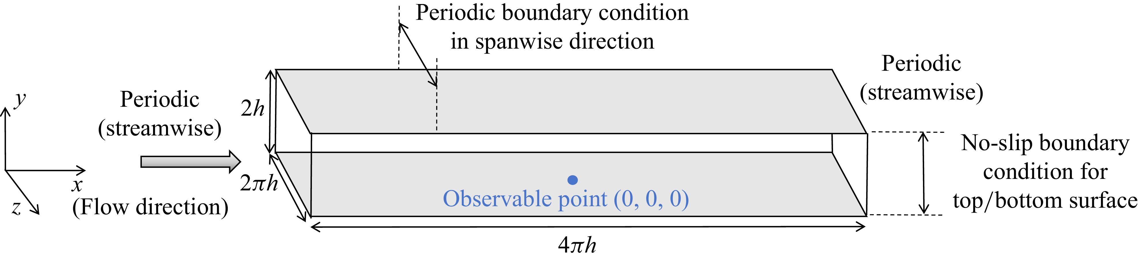
. The computational domains for all three cases remain the same, as shown in figure 1. It extends over
 $4\pi h \times 2h \times 2\pi h$
in the streamwise (
 $x$
), wall-normal (
 $y$
) and spanwise (
 $z$
) directions, respectively, where
 $h$
denotes the half-channel height. The flow is driven by a pressure gradient, which varies in time to ensure that the mass flux through the channel remains constant. The simulation time step is fixed at
 $\Delta t=0.01 h/U_b$
for the two databases of
 $Re_{\tau }\approx 180$
, while at
 $\Delta t=0.005h/U_b$
for
 $Re_{\tau }\approx 550$
. The flow snapshots are stored every 100 time steps, while the skin friction is stored every 10 time steps for all the databases.
Schematic of the computational domain, boundary conditions, coordinates and observable positions for all three DNS databases.

For the decomposition, the streamwise velocity fluctuation (time mean value removed) is chosen to represent the flow field. The observable is the skin-friction coefficient fluctuation
 $c_f^\prime$
at the centre of the bottom plate, i.e. (
 $x$
,
 $y$
,
 $z$
) =
 $(0,0,0)$
, as shown in figure 1. To improve statistical convergence in the calculation of the correlation matrix
 $\boldsymbol{A}$
, statistical homogeneity of the flow is exploited. This is because any point on the wall is equally suitable as an observable location; the associated coherent structures for all observables are identical up to a spatial shift. Thus, multiple observables may be used to improve the convergence of CCD modes (Lyu Reference Lyu2024a
). Specifically, for the observable
 $c_f^\prime$
at
 $(0,0,0)$
, the original velocity fluctuation field is used to formulate
 $\boldsymbol{U}$
, while for the observable
 $c_f^\prime$
at
 $(\pi h,0,0)$
, the velocity fluctuation field is first circularly shifted by
 $-\pi h$
in the streamwise direction before being used as an additional sample
 $\boldsymbol{U}$
in the ensemble space. In this paper, 192 and 32 such observables are used in the
 $Re_{\tau }\approx 180$
and
 $550$
cases, respectively, substantially improving the statistical convergence of the resulting CCD modes.
Note that, for CCD, the sampling frequency of the observable is independent of that of the flow. Here, it is sampled ten times faster for all databases to better resolve the temporal correlation. For example, in the uncontrolled
 $Re_\tau \approx 180$
case, a total of 16,870 observable samples are obtained, while only 1687 velocity snapshots are obtained. Since the correlation between the flow and observable is likely to decay to zero beyond a time shift of
 $10h/U_b$
, we choose
 $Q$
to be
 $100$
. Since the temporal delay between the flow and the observable is negligible, we choose
 $\tau _1$
to be
 $-5 h/U_b$
. For comparison, both the classical and extended POD are also performed.
3. Results and discussion
In this section, the CCD is applied to three DNS datasets: two uncontrolled cases at
 $Re_\tau \approx 180$
and
 $550$
, respectively, and a drag-reduction case with opposition control at
 $Re_\tau \approx 180$
. For each case, we examine the CCD spectra and the corresponding modes that are most strongly correlated with the instantaneous wall-shear stress. The spectra and mode shapes from the classical and extended POD are also briefly presented for comparison. Note that the classical POD modes are obtained in two different approaches. The first is a direct decomposition of the three-dimensional flow field, while the second aims to improve the mode convergence by first performing fast Fourier transforms (FFT) along the streamwise (
 $x$
) and spanwise (
 $z$
) directions due to statistical homogeneity, and then conducting POD in the wall-normal (
 $y$
) direction only. In the extended POD, a small subdomain in the vicinity of the observable point, i.e. the first layer of grid above the wall within the region of
 $|x|/h \lt 2\pi /3$
and
 $|z|/h\lt \pi /3$
, is used. Note that the layer directly on the wall cannot be used as it is characterised by zero velocity under the no-slip condition.
3.1. Uncontrolled cases at
 $Re_\tau \approx 180$
and
$550$


Figure 2(a,c,e,g) shows the spectra of the first 20 CCD, classical and extended POD modes for the uncontrolled
 $Re_\tau \approx 180$
case. Note that, for CCD modes, the singular values squared
 $\sigma _j^2$
measure the correlation strength between the observable and each mode, whereas for the classical and extended POD, they reflect the kinetic energy of each mode. Compared with the classical and extended POD, the CCD spectrum exhibits a much steeper decay as mode number
 $n$
increases, indicating a possibility of effective order reduction. In particular, the spectra in figure 2(c,e,g) remain comparatively flat, indicating that the kinetic energy of the classical and extended POD modes is likely to decay too slowly to yield an efficient reduced-order representation of the total flow as far as the skin friction is concerned.
The spectra and reconstruction of the skin-friction coefficient (fluctuation part) using the first 4 modes for CCD (a,b), POD (c,d), POD after FFT (e,f) and extended POD (g,h) at
 $Re_\tau \approx 180$
, respectively. Abbreviations: f-POD/FFT-POD: POD after FFT; ePOD: extended POD.

The rapid decay of the CCD spectrum suggests that the skin friction may be well approximated by a low-rank model built from only a few leading-order CCD modes. Such an attempt is demonstrated in figure 2(b), which shows reconstructions of the instantaneous skin-friction coefficient fluctuation
 $c_f^\prime$
obtained by projecting the velocity fluctuation field onto the first four CCD modes. Specifically, for flow field
 $\boldsymbol{u}_i$
at time
 $t_i$
, its projection on the
 $k$
th-order mode
 $\boldsymbol{v}_k$
is calculated by
 $a_k(t_i)=\boldsymbol{u}_i\boldsymbol{v}_k$
. Thus, an approximation of
 $\boldsymbol{u}_i$
is obtained using the linear combination of the first 4 modes, i.e.
 $\boldsymbol{u}_i^{a}=\sum ^{4}_{k=1}a_k(t_i)\boldsymbol{v}_k$
.
The skin-friction coefficient fluctuation
 $c_f^\prime$
is then reconstructed using Newton’s law by calculating the wall-normal gradient of the reconstructed streamwise velocity fluctuation at the observer point. Figure 2(b) shows that the reconstruction based on the first four CCD modes closely follows the ground truth. More specifically, the reconstruction recovers more than 80
 $\%$
of
 $c_f^\prime$
variation when measured by
 $\boldsymbol{c}_f^\prime \boldsymbol{\cdot }\boldsymbol{c}_r^\prime / |\boldsymbol{c}_f^\prime |^{2}$
, where
 $\boldsymbol{c}_f^\prime$
and
 $\boldsymbol{c}_r^\prime$
denote the true and reconstructed
 $c_f^\prime$
in vector form, respectively. As the sampling frequency of the observable increases, an even higher accuracy may be expected. In contrast, the reconstructions using the first four classical POD modes, as shown in figure 2(d,f), capture less than 2 % of the
 $c_f^\prime$
variation. This is anticipated, since POD ranks structures by kinetic energy rather than by their contribution to
 $c_f^\prime$
variations. Moreover, figure 2(h) shows that although the extended POD appears to improve the reconstruction, the improvement remains limited. If the subdomain is further reduced so as to contain only the observable point, CCD still outperforms the extended POD as it can be shown mathematically that in this case the extended POD is a degenerate case of CCD with
 $Q=1$
(Lyu Reference Lyu2024a
,
Reference Lyub
). In summary, figure 2 demonstrates that CCD provides a markedly more compact representation of the skin-friction-producing structures compared with the classical and extended POD.
Front (a,c,e,g) and left (b, d, f, h) views of the first four CCD modes at
 $Re_\tau \approx 180$
. Note that
 $z=0$
for (a, c, e, g) while
 $x=0$
for (b, f) and
 $x=\pi h/3$
for (d, h). The choice of different
 $x$
values is to show the structures in a plane with higher signal-to-noise ratios.

We are now in a position to examine the spatial structures of the resulting CCD, classical and extended POD modes. They are shown in figures 3 to 5. Note that they represent the velocity fluctuations after the mean field removed. The three decompositions yield significantly different structures in both location and organisation.
Figure 3(a,c,e,g) shows the front (
 $x$
–
 $y$
plane) views of the first four CCD modes. The CCD modes take the form of streamwise-elongated streaks whose centres are aligned with the observable location on the bottom wall. These streaks appear at a finite distance above the wall, whose centres are located at approximately
 $y^+\approx 15$
. This height is consistent with the well-established position of the buffer-layer streaks that dominate momentum transfer and near-wall shear production in canonical wall turbulence. The leading-order CCD mode exhibits the largest streamwise coherence, whereas higher-order modes display progressively shorter characteristic wavelengths, as manifested by the increasingly rapid phase variations. The streaks are also slightly inclined in the
 $x$
–
 $y$
plane, a feature commonly associated with the growth and lifting of coherent packets or hairpin-like vortical structures. Note that the skin friction can be calculated directly from the velocity gradient at the wall; therefore, since the velocity is strictly zero on the wall, a streak with an instantaneous positive sign generally corresponds to a local increase in instantaneous skin friction. Similarly, a streak with an instantaneous negative sign generally corresponds to a local decrease in instantaneous skin-friction.
Figure 3(b,d,f,h) shows the corresponding side (
 $y$
–
 $z$
plane) view of the first four CCD modes. In the spanwise direction, the CCD modes are strongly localised around the observable point at
 $z=0$
. Their effective spanwise width is approximately
 $0.2h$
, which offers a representative estimate for the spanwise scale of the streaks. This localisation indicates that only streaks sufficiently close to the observable point contribute meaningfully to the instantaneous skin friction, whereas the majority of remote structures produce a negligible contribution. Note that although the decomposition is performed using an observable at a single wall location, this does not reduce generality because the underlying flow is statistically homogeneous in both
 $x$
and
 $z$
.
Isosurface of the first- to fourth-order (a to d) CCD modes at
 $Re_\tau \approx 180$
. The red and blue isosurfaces represent
 $50\,\%$
and
 $-50\,\%$
of the fluctuation amplitude, respectively. Structures are zoomed-in in orange boxes and replotted in wall units (
 $-1000\lt x^+\lt 1000$
,
 $-100\lt z^+\lt 100$
).

To better show the structures of the resulting CCD modes, three-dimensional isosurface visualisations are shown in figure 4. These renderings reinforce the picture obtained from the planar views: the dominant CCD structures manifest as localised, streamwise-elongated streaks anchored to the vicinity of the observable point on the wall. In addition, for streaks aligned with the channel centreline, a symmetric pair of structures is observed on either side, both with an opposite phase. This pairing behaviour is consistent with the reflectional symmetry of the channel geometry and with the tendency of near-wall streaks to form in counter-rotating or phase-opposed arrangements as part of the self-sustaining cycle. Such paired streaks have been associated with the flanking motions induced by quasi-streamwise vortices, which naturally generate alternating high- and low-speed regions.
The first mode’s front and left views for POD (a, b), POD after FFT (c, d) and extended POD (e, f) at
 $Re_\tau \approx 180$
. Note that
 $z=0.6h$
for (a),
 $z=0$
for (c, e), while
 $x=0$
for (b, d, f).

In contrast, the first classical POD mode shown in figure 5(a, b) also appears as a streamwise-elongated streak, but it is neither centred around the observer location nor localised in the spanwise direction. A similar behaviour is observed for the improved classical POD modes obtained by performing FFT in advance, as shown in figure 5(c–d). This behaviour is expected because the classical POD prioritises structures that maximise kinetic-energy, rather than those most strongly associated with the
 $c_f^\prime$
variations. The second- to the fourth-order classical POD modes are similar to the first modes, and are hence omitted for brevity. Figure 5(e–f) shows the first extended POD mode. Since a small subdomain is targeted, the resulting mode appears closer to the bottom wall. However, since the extended POD modes are still optimised to capture most energy, these streaks are still scattered within the domain, particularly in the spanwise direction. These scattered patterns are even more evident in higher-order modes, which are omitted here for conciseness.
Front (a, c, e, g) and left (b, d, f, h) views of the first four CCD modes at
 $Re_\tau \approx 550$
. Note that
 $z=0$
for (a, c, e, g), while
 $x=0$
for (b, f) and
 $x=\pi h/9$
for (d, h).

As mentioned in § 1, the skin-friction-producing structures are also known to vary with Reynolds number. To assess these changes, CCD is applied to a turbulent channel flow at a higher friction Reynolds number, i.e.
 $Re_\tau \approx 550$
. The resulting first four leading-order CCD modes are shown in figure 6. Compared with the
 $Re_\tau \approx 180$
case, the mode shapes retain a broadly similar organisation and spatial distribution, suggesting that the underlying mechanism of skin-friction production remains qualitatively unchanged. Nevertheless, notable differences also exist. In particular, the streamwise and spanwise extents of the structures become significantly shorter, consistent with the well-established trend of decreasing characteristic length scales as
 $Re_\tau$
increases.
Note that these modes appear less well converged compared with those in figure 3, because fewer observables are used for the average, and the flow has a higher Reynolds number. The three-dimensional visualisations in figure 7 further demonstrate that the CCD structures decrease in size both in the
 $x$
and
 $z$
directions. A key difference, evident in figure 7(a), is that the pair of opposite-phase streaks flanking the primary streak becomes much weaker compared with figure 4(a), suggesting that, at higher Reynolds numbers, the streaks are less correlated in the spanwise direction.
Isosurface of the first- to fourth-order (a to d) CCD modes at
 $Re_\tau \approx 550$
. The red and blue isosurfaces represent
 $50\,\%$
and
 $-50\,\%$
of the fluctuation amplitude, respectively. Structures are zoomed-in in orange boxes and replotted in wall units (
 $-1000\lt x^+\lt 1000$
,
 $-100\lt z^+\lt 100$
).

Comparison of the first four CCD modes’ front views (
 $z=0$
) in wall units when
 $Re_\tau$
varies, where
 $Re_\tau \approx 180$
for (a, c, e, g) while
 $Re_\tau \approx 550$
for (b, d, f, h).

To examine the scaling of the characteristic lengths with the Reynolds number, we compare the CCD modes plotted in wall units
 $x^+$
(normalised also by
 $\nu /u_\tau$
) and
 $y^+$
at
 $Re_\tau \approx 180$
and
 $550$
, respectively, as shown in figure 8. One can see that, when plotted in wall units, the streamwise extents of the identified modes are comparable in size. The wall-normal extents appear slightly larger at
 $Re_\tau \approx 550$
; however, the difference is modest. The spanwise extents of these modes at the two Reynolds numbers are also of similar sizes. Their detailed contours in the
 $z^+$
–
 $y^+$
plane are omitted in the paper, but may be seen in the insets of figures 4 and 7, where the three-dimensional structures are shown in wall units. These imply that these optimally correlated structures follow the viscous scale near the wall.
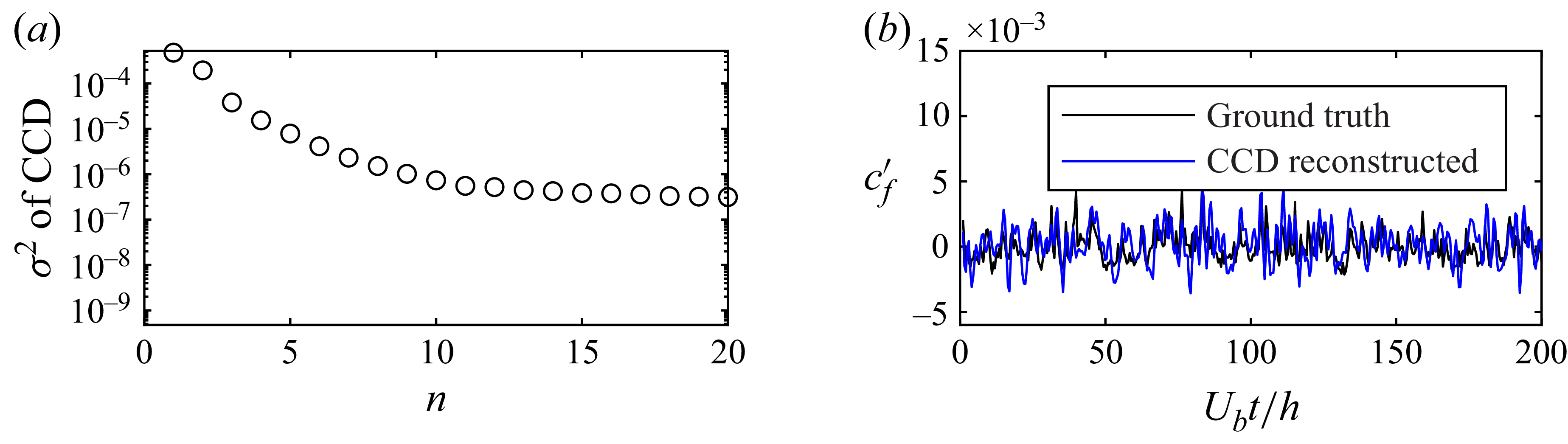
The CCD spectra and reconstruction results are shown in figures 9(a) and 9(b), respectively. Although the decay of
 $\sigma _j^2$
is somewhat slower than in the
 $Re_\tau \approx 180$
case, the first few singular values still decrease rapidly. Consequently, the reconstruction of the instantaneous skin friction remains effective, albeit being less accurate than that at
 $Re_\tau \approx 180$
. The agreement, however, is expected to improve when the observable is sampled faster.
(a) The CCD spectra and (b) reconstruction of
 $c_f\prime$
for the
 $Re_\tau \approx 550$
case.

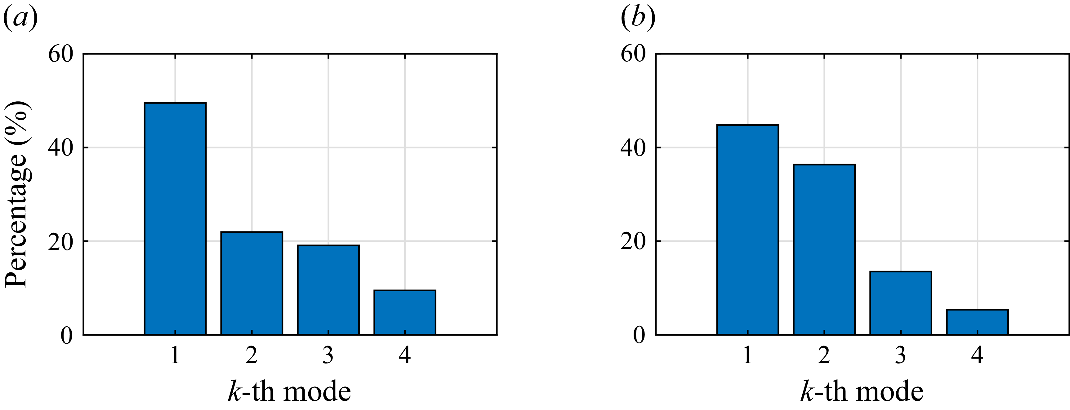
Modal contribution to the reconstructed skin-friction variation for (a)
 $Re_\tau \approx 180$
and (b)
 $550$
.

To measure the contribution of each CCD mode in the skin-friction reconstruction when
 $Re_\tau$
varies, we define the contribution ratio of the
 $k$
th-order mode as
 $\langle {a^2_k(t)}\rangle /\sum ^{4}_{n=1}\langle {a^2_n(t)}\rangle$
, where
 $\langle \rangle$
represents the time average. The results are shown in figure 10. For both
 $Re_\tau \approx 180$
and 550, the first-order mode accounts for more than 40 % of the reconstructed skin friction, indicating its leading role. As
 $Re_\tau$
increases, the second-order mode appears to show a more pronounced contribution. It is worth noting that the sampling frequency of the observable should be increased for a better mode convergence and hence a more conclusive demonstration of this trend at
 $Re_{\tau }\approx 550$
.
Front (a, c, e, g) and left (b, d, f, h) views of the first four CCD modes for the controlled flow. Note that
 $z=0$
for (a, c, e, g), while
 $x=0$
for (b, f) and
 $x=\pi h/3$
for (d, h).

Isosurface of the first- to fourth-order (a–d) CCD modes for controlled flow. The red and blue isosurfaces represent
 $50\,\%$
and
 $-50\,\%$
of the fluctuation amplitude, respectively.

3.2. Opposition-controlled case at
$Re_\tau \approx 180$

To examine the mechanism of opposition control, we apply the CCD to the controlled database at
 $Re_\tau \approx 180$
. An examination of the mean skin friction shows that a total reduction of 22
 $\%$
is achieved, consistent with prior studies of opposition control at comparable Reynolds numbers (Choi, Moin & Kim Reference Choi, Moin and Kim1994; Hammond, Bewley & Moin Reference Hammond, Bewley and Moin1998). The first four CCD modes for this case are shown in figures 11 and 12. Similar to the uncontrolled cases, the dominant structures retain streaky characteristics; however, their spatial organisation undergoes substantial modification. Most notably, the streaks are lifted farther away from the wall and show a pronounced reduction in streamwise extent. For the leading-order mode, the streamwise length of the primary streak reduces from approximately
 $9.4h$
in the uncontrolled case (figure 3
a) to
 $7h$
under control (figure 11
a). These lengths are obtained by measuring the isosurface representing 40 % of the fluctuation amplitude. This lifting and shortening of the streaks are consistent with the well-established suppression of the near-wall cycle by opposition control, wherein quasi-streamwise vortices are attenuated and the formation of elongated low-speed streaks is inhibited (Wang, Huang & Xu Reference Wang, Huang and Xu2016; Yao et al. Reference Yao, García and Hussain2025). Consequently, the coherence of near-wall streaks is reduced, resulting in more fragmented and less persistent structures.
A more significant structural change is the emergence of a secondary streak immediately beneath the primary streak, as seen in figure 11. This secondary structure is thinner, shorter and more compact – approximately half the streamwise length and one third the spanwise width of the primary streak – and exhibits an opposite phase. This feature can be interpreted as a direct imprint of the opposition actuation, which introduces anti-correlated wall-normal motions and generates counter-phase velocity responses in the near-wall region. Similar phase-opposed streaky structures have been reported in previous studies, particularly in analyses based on energy spectra and flow visualisation (Choi et al. Reference Choi, Moin and Kim1994; Wang et al. Reference Wang, Huang and Xu2016; Yao et al. Reference Yao, García and Hussain2025).
The three-dimensional visualisations in figure 12 further highlight the reorganisation of flow structures induced by opposition control. The streak system appears more interwoven and segmented than those in the uncontrolled case. In particular, the two lateral streaks flanking the primary streak become substantially more prominent – comparable in amplitude and spanwise width to the primary structure – whereas in the uncontrolled flow, they are noticeably weaker. This enhanced presence of side streaks, together with the lifted and shortened primary structure, indicates an organisation of the near-wall coherent structures that is associated with the observed skin-friction reduction.
4. Conclusion
The recently developed flow field decomposition method, CCD, is applied to turbulent channel flows to identify coherent structures most strongly associated with turbulent skin-friction generation. At
 $Re_\tau \approx 180$
, the skin-friction variation is found to correlate primarily with a set of streamwise-elongated streaks localised in the immediate spanwise vicinity of the observable point. The CCD spectrum exhibits a pronounced low-rank character: the first four modes capture more than 80 % of the skin-friction coefficient variation, in stark contrast to the negligible variation captured by the first four modes of energy-ranked decompositions such as POD and the extended POD optimised for a small subdomain in the vicinity of the observable point.
When
 $Re_\tau$
increases to
 $550$
, the CCD modes retain the same qualitative streaky structures but contract in both the streamwise and spanwise directions, consistent with the decrease of characteristic near-wall length scales at higher Reynolds numbers. Despite these quantitative differences, the underlying mechanism associated with streak-driven wall-shear production appears largely unchanged, and the extracted structures appear comparable in size when plotted in wall units. The opposition-controlled case reveals a markedly different structural organisation. The primary streaks are lifted up from the wall and become shorter in the streamwise direction. More importantly, a secondary, thinner and more compact streak of opposite phase emerges beneath each lifted streak. The three-dimensional visualisations further show a greater interweaving of streaks and enhanced prominence of flanking streaks, indicating a substantial reorganisation of near-wall coherent structures under control. Note that the structures extracted here are optimally correlated with the skin friction. They are likely to change if a different variable at the observable point is used.
These results demonstrate that CCD provides a compact and physically interpretable framework for systematically isolating the flow structures responsible for the skin-friction generation and for quantifying how these structures change under various control techniques. The structural insights obtained here offer a promising route toward an improved understanding of drag-producing mechanisms and may be used to inform the development of more effective drag-reduction techniques in wall-bounded turbulence in future work.
Funding
The authors wish to gratefully acknowledge the National Natural Science Foundation of China (NSFC) under grant numbers 12472263, U2570222.
Declaration of interests
The authors report no conflict of interest.