1 Introduction
1.1 To be or not to be
$\ldots $
 ergodic

In the nineteenth century, during his studies in the dynamical theory of gases, Ludwig Boltzmann formulated a principle that is fundamental in statistical physics—the ergodic hypothesis. This remarkable work settled the foundations of ergodic theory, an area with profound connections with analysis, probability, dynamical systems and physics. Roughly speaking, Boltzmann’s principle says that time averages equal space averages at least for typical points. Ergodicity can be formalized by saying that an automorphism
$f\colon X\rightarrow X$
 on a measure space
$(X,\unicode{x3bb} )$
 , which leaves a measure
$\unicode{x3bb} $
 invariant, must satisfy the following equality:

for
$\unicode{x3bb} $
 -almost every (a.e.)
$x\in X$
 and any continuous observable
$\varphi \colon X\rightarrow \mathbb {R}$
 .
Another equivalent definition of ergodicity says that any f invariant set must have zero or full
$\unicode{x3bb} $
 -measure. In this paper, we will be interested in the case where
$\unicode{x3bb} $
 is the volume measure. Whenever we consider perturbations of volume-preserving maps (also called conservative), we assume that they still keep the volume invariant. We say that a property is generic (or residual) if it holds in a set that contains a countable intersection of open and dense subsets. In a Baire space, a generic set is dense.
Some central questions in conservative dynamics include determining whether a given map is ergodic, stably ergodic or becomes ergodic after a small perturbation. A map is stably ergodic if ergodicity prevails even after small perturbations. The answers to these questions can vary significantly depending on the topology used to compare maps. In fact, we have the following facts.
-
(i) The ergodic conservative homeomorphisms are $C^0$
-generic. This was proved in the celebrated paper by Oxtoby and Ulam [Reference Oxtoby and Ulam21]. In particular, any
$C^0$
homeomorphism can be
$C^0$
approximated by an ergodic one. Yet, there is no possible way to get
$C^0$
-open sets of ergodic homeomorphisms, since the
$C^0$
-topology, as being really very feeble, allows us to destroy ergodic maps under
$C^0$
-perturbations. The techniques to get
$C^0$
-genericity of ergodicity in [Reference Oxtoby and Ulam21] were pushforward by Krengel in [Reference Krengel16] to get
$C^0$
-genericity of zero metric entropy. -
(ii) There are examples of $C^1$
-open sets of conservative diffeomorphisms, the Anosov ones, such that all the elements of the open set are ergodic with respect to volume [Reference Anosov5]. In this case, we have stable ergodicity and stable positive metric entropy. However, Anosov maps are far from being typical. Furthermore, trying to adapt the arguments in [Reference Oxtoby and Ulam21] to the
$C^1$
topology and obtain
$C^1$
-genericity of ergodicity is doomed to failure because, similarly, we could also obtain
$C^1$
-genericity of zero metric entropy, which is false as we saw earlier. -
(iii) There are examples of $C^r$
-open sets of diffeomorphism (
$r>3$
) such that there are no ergodic maps in the open set. These examples, eventually with more regularity, are known since the mid-20th century from the outstanding work by Kolmogorov, Arnold and Moser (KAM). This tuning on the regularity for
$C^r$
(
$r>3$
) was provided by Yoccoz [Reference Yoccoz26]. These KAM examples ended Boltzmann’s dream on fulfilling the ergodic hypothesis for most maps.


In the title of the Oxtoby and Ulam paper [Reference Oxtoby and Ulam21], ergodicity is referred to by the outdated expression metrical transitivity. This can be contextualized noticing that ergodicity displays a kind of measure indecomposability of the phase space. There is another type of indecomposability with topological flavour called topological transitivity, which means that the dynamical system displays a dense orbit in the whole manifold. Regarding the generic theory of topological transitivity, we have that both:
-
(iv) $C^0$
-generic conservative homeomorphisms are topological transitive [Reference Alpern and Prasad3]; and -
(v) $C^1$
-generic conservative diffeomorphisms are topological transitive [Reference Bonatti and Crovisier8].


Throughout the article, X is a smooth closed connected Riemannian manifold of dimension
$d\geq 2$
 .
1.2 The Sobolev class
Items (i)–(iii) above reveal that there is a clear change of paradigm from
$C^0$
 to
$C^1$
 and from
$C^1$
 to
$C^3$
 . We are interested in complementing the literature concerning the genericity of ergodicity, focusing on the first jump. Moreover, items (iv) and (v) above show that topological transitivity prevails generically both
$C^0$
 and
$C^1$
 . We will also extend these generic results to the following Sobolev framework.
First, we need to define, given an open bounded subset
$\Omega $
 of
$\mathbb {R}^d$
 , a Baire space with a topology capturing the uniform and the
$(1,p)$
 -Sobolev topologies (
$0<p<\infty $
 ), where we will look for the ergodic or the topologically transitive elements. With this in mind, we consider
$W^{1;\infty ,p}(\Omega ,\mathbb {R}^d)$
 , the completion of the space of the
$C^1$
 functions, continuous on
$\overline {\Omega }$
 , admitting derivatives in
$L^p(\Omega )$
 , relative to the norm
$\|\,{\cdot}\, \|_{1;\infty ,p}=\max \{\|\,{\cdot}\, \|_\infty ,\|\,{\cdot}\, \|_{1,p}\}$
 . Formally, an element
$f\in W^{1;\infty ,p}(\Omega ,\mathbb {R}^d)$
 is represented by a pair
$(\pi _1(f),\pi _2(f))$
 , with
$\pi _1(f)$
 being the uniform limit of a sequence and
$\pi _2(f)$
 the limit in
$L^p(\Omega )^{d^2}$
 of the sequence of their derivatives.
If
$p\geq 1$
 , then a pair in
$W^{1;\infty ,p}(\Omega ,\mathbb {R}^d)$
 is identified by its first coordinate, as its derivative is the second one. With this in mind, it can be shown that
$W^{1;\infty ,p}(\Omega ,\mathbb {R}^d)$
 is formed by the continuous functions from
$\overline {\Omega }$
 to
$\mathbb {R}^d$
 admitting distributional derivatives in
$L^p(\Omega )$
 . In contrast to the
$C^0$
 and
$C^1$
 case, if
$f,g\in W^{1;\infty ,p}(\Omega ,\mathbb {R}^d)$
 and
$f(\overline {\Omega })\subseteq \overline {\Omega }$
 , then
$g\circ f$
 may not belong to
$W^{1;\infty ,p}(\Omega ,\mathbb {R}^d)$
 . For that reason, we consider
$\overline {\textrm {Lip}_\unicode{x3bb} (\Omega )}^{\,p}$
 as the closure of the conservative Lipschitz homeomorphisms. Finally, we consider
$\mathcal {M}^{1,p}_\unicode{x3bb} (\Omega )$
 as the space of the homeomorphisms in
$\overline {\textrm {Lip}_\unicode{x3bb} (\Omega )}^{\,p}$
 , which is a Baire space.
If
$0<p<1$
 , the situation is different as if
$f\in W^{1;\infty ,p}(\Omega ,\mathbb {R}^d)$
 ,
$\pi _2(f)$
 may not be the derivative of
$\pi _1(f)$
 . For this reason, we have to adapt the definitions above, essentially calling a pair a bijection/conservative/Lipschitz/homeomorphism/ergodic if its first coordinate is.
For full details, see §2.2.
These concepts can be carried over to a smooth closed connected manifold.
Our main goal is to obtain a version of the Oxtoby–Ulam theorem establishing that ergodicity is generic, for
$0<p<1$
 (Theorem B), and that topological transitivity is also generic, for
$1\leq p<d-1$
 (Theorem C).
We observe that Sobolev homeomorphisms have gained particular significance in various applications, such as certain types of partial differentiential equations (PDEs) in nonlinear elasticity (see the Ball–Evans problem in [Reference Iwaniec, Kovalev and Onnine15]), in ergodic theory (genericity of infinite topological entropy in [Reference de Faria, Hazard and Tresser11, Reference de Faria, Hazard and Tresser12]), in dynamical systems related to the closing lemma [Reference Azevedo, Azevedo, Bessa and Torres7, Reference de Faria, Hazard and Tresser12] and in global analysis [Reference Azevedo, Azevedo, Bessa and Torres6, Reference de Faria and Hazard10].
1.3 A volume-preserving Sobolev Lusin theorem
The Lusin theorem was summed up by J. E. Littlewood by saying that ‘every measurable function is nearly continuous’.
In Theorem A, we obtain a weak version of Lusin’s theorem in the Sobolev-
$(1,p)$
 uniform closure of volume-preserving Lipschitz homeomorphisms on closed and connected d-dimensional manifolds,
$d \geq 2$
 and
$0<p<1$
 .
This result generalizes for the Sobolev setting previous
$C^0$
 versions proved by Oxtoby [Reference Oxtoby19], White [Reference White24], Alpern and Prasad [Reference Alpern and Prasad3], and Alpern and Edwards [Reference Alpern and Edwards2].
We point out that Theorem A is the crucial ingredient that allow us, in Theorem B, to obtain a version of the Oxtoby–Ulam theorem.
Let
$\mathcal {G}_\unicode{x3bb} (X)$
 denote the set of measurable bijections on X that keep
$\unicode{x3bb} $
 invariant.
Theorem A. (Volume-preserving Sobolev weak Lusin theorem)
Let X be a closed connected d-dimensional manifold,
$d \geq 2$
 and
$0<p<1$
 . Let
$g \in \mathcal {G}_\unicode{x3bb} (X)$
 ,
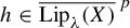
$h\in \overline {\mathrm {Lip}_\unicode{x3bb} (X)}^{\,p}$
 and consider
$\delta>0$
 . Then, given any weak topology neighbourhood
$\mathcal {W}$
 of g, there exists
$f \in \mathrm {Lip}_\unicode{x3bb} (X)$
 such that
$f \in \mathcal {W}$
 and

1.4 Towards the Oxtoby–Ulam theorem
In addition to its intrinsic importance in analysis, the weak Lusin theorem in the volume-preserving class was crucial in a proof given in [Reference Alpern and Prasad3] of the result of Oxtoby and Ulam, that ergodicity is generic for measure-preserving homeomorphisms of compact manifolds. Therefore, a Sobolev version of this theorem (cf. Theorem A) will be useful in the study of dynamical properties in the Sobolev class.
Our main result is the generalization of the important classic Oxtoby–Ulam theorem for
$\mathcal {M}^{1,p}_\unicode{x3bb} (X)$
 .
We say that an element
$f\in \mathcal {M}^{1,p}_\unicode{x3bb} (X)$
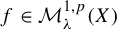 is ergodic if
$\pi _1(f)$
 is ergodic.
Theorem B. (Sobolev Oxtoby–Ulam theorem)
Let X be a closed connected d-dimensional manifold,
$d \geq 2$
 and
$0< p<1$
 . The set of the ergodic elements in
$\mathcal {M}^{1,p}_\unicode{x3bb} (X)$
 is generic.
We cannot fail to mention to the reader the obligation to look through the beautiful written historical background in [Reference Alpern and Prasad4, §1] describing the trajectory of, undoubtedly, one of the most important results in dynamical systems.
1.5 Genericity of topological transitivity
We say that a homeomorphism f is topologically transitive if given any open sets
$U,V\subset X$
 , we have

Since ergodicity is stronger than topological transitivity, a direct corollary of Theorem B states that the topologically transitive elements in
$\overline {\textrm {Lip}_\unicode{x3bb} (X)}^{\,p}$
 ,
$0< p<1$
 , form a residual set. However, the problem of genericity of ergodicity for
$p\geq 1$
 remains unsolved. Our last result is a topological counterpart of the Oxtoby–Ulam theorem (topological transitivity instead of metric transitivity) for
$\mathcal {M}^{1,p}_\unicode{x3bb} (X)$
 ,
$p\geq 1$
 .
Theorem C. (Sobolev generic transitivity)
Let X be a closed connected d- dimensional manifold,
$d \geq 3$
 and
$1\leq p<d-1$
 . The topologically transitive elements in
$\mathcal {M}^{1,p}_\unicode{x3bb} (X)$
 form a generic set.
1.6 Open problems
We end the introduction by considering several important open questions. In [Reference de Faria, Hazard and Tresser11], the early result by Yano [Reference Yano25] in the 1980s was generalized for Sobolev homeomorphisms. We ask if an analogous result holds in the conservative class posing the following problem.
Problem 1. Is infinite topological entropy generic in
$\mathcal {M}^{1,p}_\unicode{x3bb} (X)$
 for
$p>0$
 ?
The seminal ideas from Oxtoby and Ulam’s paper [Reference Oxtoby and Ulam21] on periodic approximations can be used to obtain
$C^0$
 -genericity of zero metric entropy (see [Reference Choksi and Prasad9, Reference Krengel16, Reference Rohlin23]). With this in mind, we consider the following question.
Problem 2. Is zero metric entropy generic in
$\mathcal {M}^{1,p}_\unicode{x3bb} (X)$
 for
$p>0$
 ?
An affirmative answer to previous problems would allow us to conclude that the volume measure could not play an effective role on fulfilling an (hypothetical) variational principle for a generic set of Sobolev conservative homeomorphisms.
Finally, we pose what we believe to be the most important open question.
Problem 3. Is ergodicity generic in
$\mathcal {M}^{1,p}_\unicode{x3bb} (X)$
 for
$p\geq 1$
 ?
This paper is organized as follows. In §2, we introduce the space of automorphisms and the Sobolev-
$(1,p)$
 framework in which we will work (
$0<p<\infty $
 ). In §3, we prove a key perturbation result (Theorem 3.1) which will be crucial to prove the theorems of the subsequent sections. In §4, we obtain a weak version of Lusin’s theorem for
$p<1$
 (Theorem A). In §5, we prove the Sobolev Oxtoby–Ulam theorem (Theorem B) with respect to the same topology. In §6, we prove the genericity of topological transitivity (Theorem C) for
$1\leq p<d-1$
 . Finally, in §7, we construct an explicit example showing that the space
$\mathcal {M}^{1,p}_\unicode{x3bb} (X)$
 is not a functional one.
2 Preliminaries
We recall that X is a smooth closed connected Riemannian manifold of dimension d and
$d_X$
 is the distance on X induced by the Riemannian structure. We denote the Euclidean norm in
$\mathbb {R}^d$
 by
$|\cdot |$
 . Let
$\unicode{x3bb} $
 stand for the measure on both X and
$\mathbb {R}^d$
 derived from the standard volume form.
2.1 Automorphisms and homeomorphisms of
$(X,\unicode{x3bb} )$

An automorphism of the underlying Borel measure space
$(X,\unicode{x3bb} )$
 is a bijection
$g \colon X \to X$
 such that g and, consequently,
$g^{-1}$
 are measurable functions and
$\unicode{x3bb} (B)=\unicode{x3bb} (g^{-1}(B))$
 for all measurable sets B. Automorphisms that differ on a set of measure zero will be identified. We denote by
$\mathcal {G}_\unicode{x3bb} (X)$
 the space of automorphisms of
$(X,\unicode{x3bb} )$
 . We shall consider two topologies on
$\mathcal {G}_\unicode{x3bb} (X)$
 .
The first, defined by Halmos [Reference Halmos13], requires that a sequence
$(f_n)_n$
 converges to f if and only if
$\lim _n\unicode{x3bb} (f_n(A)\triangle f(A))=0$
 for every measurable
$A\subseteq X$
 (here,
$\triangle $
 means ‘symmetric difference’). In [Reference Halmos14, pp. 62–64], Halmos proved that
$\mathcal {G}_\unicode{x3bb} (X)$
 endowed with the weak topology is a topological group and is topologically complete. In particular,
$\mathcal {G}_\unicode{x3bb} (X)$
 with the weak topology is a Baire space. In addition, Alpern proved in [Reference Alpern1] that the weak topology is determined by the metric, known as weak metric, defined by

This metric will be used, for instance, in the proof of Theorem A.
The second topology we consider over
$\mathcal {G}_\unicode{x3bb} (X)$
 is the uniform topology determined by the metric defined by

The space
$\mathcal {G}_\unicode{x3bb} (X)$
 with the uniform topology is a Baire space.
We denote by
$\mathcal {M}_\unicode{x3bb} (X)$
 the subspace of all homeomorphisms in
$\mathcal {G}_\unicode{x3bb} (X)$
 , endowed with the uniform topology. This space is not complete, but it is topologically complete (see [Reference Oxtoby20]), and thus a Baire space. In fact, as X is compact, the metric is equivalent to the complete metric defined by

We shall call volume-preserving homeomorphisms of X the elements in
$\mathcal {M}_\unicode{x3bb} (X)$
 . For
$f\in \mathcal {M}_\unicode{x3bb} (X)$
 and
$\delta>0$
 , we shall denote by
$B^\infty (f,\delta )$
 the uniform ball centred in f and with radius
$\delta $
 .
2.2 Sobolev maps
Let
$\Omega $
 be an open bounded subset of
$\mathbb {R}^d$
 and
$0<p <\infty $
 . It is well known that
$L^p(\Omega )$
 endowed with its natural norm or quasi-norm for
$1\leq p< \infty $
 or
$0<p<1$
 , respectively, defined by

is a complete space.
Indeed, for
$0<p<1$
 , from the inequality
$(a+b)^p\leq a^p+b^p$
 , for
$a,b\geq 0$
 , we obtain

proving that
$L^p(\Omega )$
 is a metric space. Therefore, we have the quasi-triangle inequality as

In contrast to the case where
$1\leq p<\infty $
 , if
$0<p<1$
 ,
$L^p(\Omega )$
 is neither a normable nor a locally convex space, from where one can obtain that its dual is the trivial space.
Of course, if
$\Omega $
 is bounded and
$0<p<q<\infty $
 , then
$L^q(\Omega )$
 is continuously included in
$L^p(\Omega )$
 . In fact, if
$f\in L^q(\Omega )$
 , we have, using the Hölder inequality,

For
$1\leq p<\infty $
 , there are (usually) two equivalent ways to define the Sobolev spaces
$W^{n,p}(\Omega )$
 [Reference Meyers and Serrin17]: one using a completion of
$C^n(\Omega )$
 and the other using weak derivatives of functions in
$L^p(\Omega )$
 . If
$0<p<1$
 , only the first one has a sense because, for those p, a function in
$L^p(\Omega )$
 may not be locally integrable.
For
$0<p<1$
 , the completion
$W^{n,p}(\Omega )$
 has a strange behaviour. For simplicity, let us look at the case where
$n=d=1$
 ,
$\Omega $
 being an interval. Peetre [Reference Peetre22] proved that for all
$g,h\in L^p(\Omega )$
 , there exists an element of
$W^{1,p}(\Omega )$
 represented by a sequence
$(f_n)_n$
 such that

That is, in this case, the elements of
$W^{1,p}(\Omega )$
 are represented by pairs
$(g,h)\in L^p(\Omega )\times L^p(\Omega )$
 , where h can be any function in
$L^p(\Omega )$
 and not necessarily the weak derivative of g, as happens if
$p\geq 1$
 .
Just to give an idea of what is possible in this space, we present an explicit example (adapted from [Reference Peetre22]) of this situation.
Example 2.1. For
$n\in \mathbb {N}$
 , let
$a,b>0$
 with
$a+b={1}/{n}$
 and consider
$f_n:[0,{1}/{n}]\rightarrow [0,{1}/{n}]$
 defined by

We extend
$f_n$
 to a function from
$[0,1]$
 to
$[0,1]$
 defining
$f_n({k}/{n}+x)=f_n(x) +{k}/{n}$
 if
$x\in\ ] {k}/{n},({k+1})/{n}]$
 , with
$k\in \{0,1\ldots ,n-1\}$
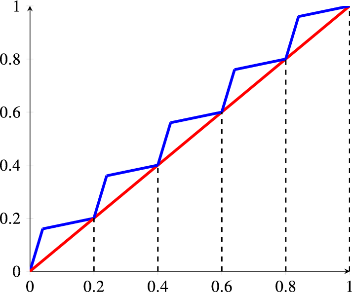
 (see Figure 1). Note that these functions are Lipschitz homeomorphisms.
Graphic of
$f_5$
 (with
$a={1}/{25}$
 ) and of the identity (colour online).

Let I be the identity function in
$[0,1]$
 . Then,
$\|f_n-I\|_\infty \leq {1}/{n}$
 , proving that
$ (f_n)_n$
 converges uniformly and in all
$L^p(I)$
 , for
$0<p<\infty $
 . If we fix
$0<p<1$
 , then

If we choose a such that
$\lim _n an=0$
 (or
$\lim _nbn=0$
 ), then
$(f_n)_n$
 converges in
$W^{1,p}(I)$
 to an element f represented by the pair
$(I,0)$
 .
In the present paper, all the functions we will be interested in are volume-preserving homeomorphisms from
$\overline {\Omega }$
 to
$\overline {\Omega }$
 , whose components are in
$W^{1,p}(\Omega )$
 .
With this in mind, we start with the vectorial space

with the norm or quasi-norm for
$1\leq p<\infty $
 or
$0<p<1$
 , respectively, defined by

where
$\|f\|_\infty =\max _i\|f_i\|_\infty $
 and
$\|Df\|_{p}=\max _{i,j}\|{\partial f_i}/{\partial {x_j}}\|_p$
 .
Note that we do not need to include
$\|f\|_p$
 in (2.4), as it is superfluous.
Definition 2.1. If
$\Omega $
 is an open bounded subset of
$\mathbb {R}^d$
 and
$0<p<\infty $
 , we denote by
$W^{1;\infty ,p}(\Omega ,\mathbb {R}^d)$
 the completion of the space defined in (2.3) relative to the norm
$\|\,{\cdot}\, \|_{1;\infty ,p}$
 .
As in any completion, if
$f\in W^{1;\infty ,p}(\Omega ,\mathbb {R}^d)$
 , we denote by
$\|f\|_{1;\infty ,p}$
 the limit of the sequence
$(\|f_n\|_{1;\infty ,p})_n$
 , where
$(f_n)_n$
 is a representative Cauchy sequence of f.
Remark 2.2. Notice that, using (2.2), if
$0<p<q<\infty $
 , then
$W^{1;\infty ,q}(\Omega ,\mathbb {R}^d)$
 is continuously included in
$W^{1;\infty ,p}(\Omega ,\mathbb {R}^d)$
 .
An element of
$f\in W^{1;\infty ,p}(\Omega ,\mathbb {R}^d)$
 is represented by a Cauchy sequence
$(f_n)_n$
 relatively to the norm defined in (2.4). Thus, the sequences
$(f_n)_n$
 and
$(D f_n)_n$
 are Cauchy (and then convergent) sequences in
$C^0(\overline {\Omega })^d$
 and
$(L^p(\Omega ))^{d^2}$
 , respectively. Then, we have a linear continuous inclusion

and

As noted before, in [Reference Meyers and Serrin17], if
$p\geq 1$
 , then
$\pi _2(f)$
 is the weak derivative of
$\pi _1(f)$
 and, then, f will be represented only by
$\pi _1(f)$
 . Furthermore, if
$u\in L^p(\Omega )^d$
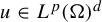 admitting weak partial derivatives in
$L^p(\Omega )$
 , then, there not only exists a sequence of
$C^\infty $
 functions converging to u in
$W^{1,p}(\Omega ,\mathbb {R}^d)$
 , but also in
$C^0(\overline {\Omega })^d$
 , if
$u\in C^0(\overline {\Omega })^d$
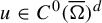 . Then,

where the derivatives are weak ones.
Example 2.3. If
$f_n$
 is defined as in Example 2.1 and

then
$(F_n)_n$
 is a sequence of homeomorphisms converging uniformly to the identity I and
$(DF_n)_n$
 converges to the null function in
$L^p(I^d)^{d^2}$
 . So, the limit of
$(F_n)_n$
 in
$W^{1;\infty ,p}(\Omega ,\mathbb {R}^d)$
 is represented by the pair
$(I,0)$
 and, of course, the second component is not the derivative of the first one.
Using (2.6) and Remark 2.2, it follows that the Lipschitz functions from
$\overline {\Omega }$
 to
$\overline {\Omega }$
 belong to
$W^{1;\infty ,p}(\Omega ,\mathbb {R}^d)$
 for every
$0<p<\infty $
 . Consequently, the following definition makes sense.
Definition 2.2. If
$\Omega $
 is a bounded open subset of
$\mathbb {R}^d$
 and
$0<p<\infty $
 , let
$\textrm {Lip}_\unicode{x3bb} (\Omega )$
 be the subspace of
$W^{1;\infty ,p}(\Omega ,\mathbb {R}^d)$
 formed by the volume-preserving Lipschitz homeomorphisms from
$\overline {\Omega }$
 to
$\overline {\Omega }$
 . The closure in
$W^{1;\infty ,p}(\Omega ,\mathbb {R}^d)$
 of
$\textrm {Lip}_\unicode{x3bb} (\Omega )$
 will be denoted by
$\overline {\textrm {Lip}_\unicode{x3bb} (\Omega )}^{\,p}$
 .
Remark 2.4. If
$f\in \overline {\textrm {Lip}_\unicode{x3bb} (\Omega )}^{\,p}$
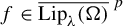 , then
$\pi _1(f)\in C^0_\unicode{x3bb} (\overline {\Omega })$
 , the set of volume-preserving functions, but it may not be a homeomorphism. However, if
$\pi _1(f)$
 , it is injective and then it is a homeomorphism.
This justifies the definition of the Baire space with which we are going to work.
Definition 2.3. If
$\Omega $
 is a bounded open subset of
$\mathbb {R}^d$
 and
$0<p<\infty $
 , we denote by
$\mathcal {M}^{1,p}_\unicode{x3bb} (\Omega )$
 the subspace of
$\overline {\textrm {Lip}_\unicode{x3bb} (\Omega )}^{\,p}$
 ,

It is clear that, if we have an element
$f=(g,h)\in \mathcal {M}^{1,p}_\unicode{x3bb} (\Omega )$
 then, viewing h as a matrix
$d\times d$
 , the determinant of h is, almost everywhere, equal to
$\pm 1$
 . This is a consequence of the fact that the
$L^p$
 convergence implies almost everywhere convergence and that g is the limit in
$L^p(\Omega )^{d^2}$
 of a sequence in
$\textrm {Lip}_\unicode{x3bb} (\Omega )$
 . In particular, the element
$(I,0)$
 defined in Example 2.3 does not belong to
$\mathcal {M}^{1,p}_\unicode{x3bb} (\Omega )$
 .
It is natural to ask if
$\mathcal {M}^{1,p}_\unicode{x3bb} (I^d)$
 contains any element
$f=(g,h)\in \mathcal {M}^{1,p}_\unicode{x3bb} (I^d)$
 such that h is not the weak derivative of g. Of course, the question only makes sense if
$0<p<1$
 . In §7, we answered positively to this question using techniques that will be developed in the following sections.
Proposition 2.5. If
$\Omega $
 is a bounded open subset of
$\kern1.2pt\mathbb {R}^d$
 and
$0<p<\infty $
 , then
$\mathcal {M}^{1,p}_\unicode{x3bb} (\Omega )$
 is a Baire space.
Proof. Let

Using Remark 2.4, it is clear that
$\mathcal {M}^{1,p}_\unicode{x3bb} (\Omega )=\bigcap _n X_n$
 . To conclude the proof, it is enough to show that, for
$n\in \mathbb {N}$
 ,
$X_n$
 is an open subset of
$\overline {\textrm {Lip}_\unicode{x3bb} (X)}^{\,p}$
 , which is a complete space.
Given
$f\in X_n$
 , let

As
$\overline {\Omega }$
 is compact, then
$\delta> 0$
 . Let us see that, if
$g\in \overline {\textrm {Lip}_\unicode{x3bb} (\Omega )}^{\,p}$
 and
$\|f-g\|_{1;\infty ,p}<{\delta }/{2}$
 , then
$g\in X_n$
 . In fact, if
$x,y\in \overline {\Omega }$
 and
$|x-y|\geq {1}/{n}$
 , then, as
$\|f-g\|_\infty \leq \|f-g\|_{1;\infty ,p}$
 ,

from where we conclude that
$\pi _1(g)(x)\neq \pi _1(g)(y)$
 and then
$g\in X_n$
 .
The following result will be useful in the proof of Theorems A and C to estimate the
$L^p$
 -norm of the derivative of some composition of functions.
Lemma 2.6. Let
$f,g:I^d\rightarrow I^d$
 be Lipschitz functions, with g being a volume-preserving homeomorphism. If
$M=\max _{i,j}\|{\partial g_i}/{\partial x_j}\|_\infty $
 and
$p>0$
 , then

Proof. Using the chain rule, we have

Then, as g is measure-preserving,

If
$p\geq 1$
 , the triangular inequality gives

If
$0<p<1$
 , using (2.1), we obtain

and the conclusion follows.
All these concepts can be carried over to a smooth closed connected manifold.
3 A key perturbation theorem
The next theorem will serve as a cornerstone result essential for establishing a volume-preserving Sobolev weak Lusin theorem and the generic results of the following sections. Here,
$I^d=[0,1]^d$
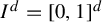 denotes the d-dimensional unit cube.
Theorem 3.1. Let
$d \geq 2$
 ,
$0<p<d-1$
 ,
$N\in \mathbb {N}$
 , and consider
$ \{P_i\}_{i=1}^N$
 and
$\{Q_i\}_{i=1}^N$
 as two sets of N distinct interior points of
$I^d$
 .
For sufficiently small
$r>0$
 , there is F, a volume-preserving
$C^{\infty }$
 diffeomorphism of
$I^d$
 , equal to the identity outside
$I^d$
 and in a neighbourhood of the boundary of
$I^d$
 , which sends, by translation, a ball of radius r centred in
$P_i$
 onto a ball centred in
$Q_i$
 .
Moreover, if
$\delta>0$
 , we can choose r such that

Remark 3.2. In the previous theorem, the function F will actually be equal to the identity outside a finite union of tubular neighbourhoods of ellipses of radius chosen as small as we need.
Remark 3.3. The conclusion of the previous theorem is false if
$p>d$
 , unless
$P_i=Q_i$
 for all
$i=1,\ldots ,N$
 . In fact, that conclusion would imply the existence of a sequence
$(F_n)_n$
 of functions converging to
$I_d$
 in
$W^{1,p}(I^d,I^d)$
 and such that the sequence
$(\|F_n-\mathrm {Id}\|_\infty )_n $
 converges to
$\max _i|P_1-Q_i|$
 , which contradicts the continuous inclusion of
$C^0(I^d)$
 in
$W^{1,p}(I^d)$
 , for those p.
The remainder of this section is devoted to proving Theorem 3.1.
3.1 Pseudo-ring
We introduce the following notion. Let
$\mathcal {E}$
 be an ellipse (not reduced to a point). Then, there exist unique b and R, with
$0\leq b\leq 1$
 and
$R> 0$
 , such that in a certain orthonormal basis of
$\mathbb {R}^d$
 , after a translation, the equations of the ellipse are
${x_1^2+({x_2}/{b})^2=R^2}$
 ,
$x_i=0$
 , for
$i\geq 3$
 .
For
$r>0$
 , we denote by
$\mathit{PR}^{\mathcal {E}}_r$
 the set, in the new variables,

We call this set a pseudo-ring in
$\mathbb {R}^d$
 as, if
$b=1$
 and
$R>r>0$
 , it is a d-ring, that is, obtained by the rotation of a
$d-1$
 ball of radius r around a circle of radius R. Notice that if
$R>r>0$
 , then, denoting by
$\omega _{d-1}$
 the volume of the unit ball in
$\mathbb {R}^{d-1}$
 ,

If
$b<1$
 , then
$\mathit{PR}^{\mathcal {E}}_r$
 is not a tubular neighbourhood of
$\mathcal {E}$
 , but is contained and contains tubular neighbourhoods of
$\mathcal {E}$
 . We denote by
$D(\mathcal {E},s)$
 , for
$s>0$
 , the closed tubular neighbourhood of
$\mathcal {E}$
 of radius s.
Lemma 3.4. In the previous conditions,

In particular, the disk
$D((\pm R,0,\ldots ,0),br)$
 is contained in
$\mathit{PR}^{\mathcal {E}}_r$
 .
Proof. We only need to consider the case
$d=2$
 .
Let
$x=(x_1,x_2)\in \mathit{PR}^{\mathcal {E}}_r$
 and consider
$\xi =\sqrt {x_1^2+({x_2}/{b})^2}$
 ,
$y=({R}/{\xi })(x_1,x_2)\in \mathcal {E}$
 . Then,

proving that
$x\in D(\mathcal {E},r)$
 .
However, let
$(x_1,x_2)\in D(\mathcal {E},br)$
 and consider
$(\alpha ,\beta )\in \mathcal {E}$
 such that
$\|(x_1,x_2)-(\alpha ,\beta )\|_2\leq br$
 . Then,
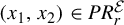
$(x_1,x_2)\in \mathit{PR}^{\mathcal {E}}_r$
 , as

As a particular case, noticing that
$(\pm R,0)\in \mathcal {E}$
 , we obtain
$D((\pm R,0),br)\subseteq \mathit{PR}^{\mathcal {E}}_r$
 .
3.2 Proof of Theorem 3.1
We start by proving some auxiliary results.
Lemma 3.5. Let
$d\geq 2$
 ,
$b>0$
 ,
$Z:\mathbb {R}^{d-1}\rightarrow \mathbb {R}$
 be a differentiable function and consider
$\alpha : \mathbb {R}^d \longrightarrow \mathbb {R}$
 defined by
$\alpha (x)=Z(x_1^2+({x_2}/{b})^2,\bar x)$
 , where
$\bar x=(x_3,\ldots ,x_d)$
 .
Then, the function
$F_b^\alpha : \mathbb {R}^d \rightarrow \mathbb {R}^d$
 defined by

is a volume-preserving diffeomorphism, with the same differential regularity as Z.
Proof. Note that writing
$F_b^\alpha =F=(F_1,\ldots ,F_d)$
 , we have

and then

However, as

then
$\alpha (x)=\alpha (F_b^\alpha (x))$
 . Therefore, it is easy to see that the inverse of
$ F_b^\alpha $
 is
$ F_b^{-\alpha }$
 .
Given
$\mu \in \,] 0,1[$
 , let
$h_\mu :\mathbb {R}\rightarrow \mathbb {R}$
 be a
$C^\infty $
 function, equal to
$\pi $
 in
$]{-}\infty ,1-\mu ] $
 , strictly decreasing in
$]1-\mu ,1[$
 and equal to
$0$
 in
$[1,+\infty [$
 . An explicit example of a function
$h_\mu $
 is defined in
$]1-\mu ,1[$
 by

As
$h_\mu '$
 is zero outside
$[1-\mu ,1]$
 and
$h_\mu '$
 is continuous, then
$|h_\mu '|$
 is bounded by a constant
$C=C(\mu )$
 . As a curiosity, one can verify that the best constant is
${2\pi }/{\mu }$
 .
Lemma 3.6. Let
$d\geq 2$
 and consider an ellipse
$\mathcal {E}$
 . Then, for
$r>0$
 , there exists
${F:\mathbb {R}^d\rightarrow \mathbb {R}^d}$
 , a volume-preserving
$C^\infty $
 diffeomorphism, which is equal to the identity outside
$\mathit{PR}^{\mathcal {E}}_r$
 , and in
$\mathit{PR}^{\mathcal {E}}_{({r}/{2})}$
 is a rotation of an angle
$\pi $
 in the plane of the ellipse whose centre is the centre of the ellipse.
Moreover, for
$r>0$
 , there exists C, increasing with r, such that
$|({\partial F_i}/{\partial x_j})(x)|\leq {C}/{r}$
 for all
$i,j=1,\ldots ,d$
 and
$x\in \mathbb {R}^d$
 .
Proof. Using a translation followed by a linear function with determinant equal to
$1$
 , we can suppose that the ellipse has equations
$x_1^2+({x_2}/{b})^2=R^2$
 ,
$x_i=0$
 , for
$i\geq 3$
 , for some
$b>0$
 .
Denote
$h_{\frac 34}$
 by h, consider
$\alpha :\mathbb {R}^d\rightarrow \mathbb {R}$
 defined by

and F defined in Lemma 3.5, for this function
$\alpha $
 . If
$x\notin \mathit{PR}^{\mathcal {E}}_r$
 , then
$\alpha (x)=0$
 and so
${F(x)=x}$
 . If
$x\in \mathit{PR}^{\mathcal {E}}_{{r}/{2}}$
 , then
$\alpha (x)=\pi $
 and
$F(x)=(-x_1,-x_2,\bar x)$
 .
For the second part, we only need to consider points in the interior of
$\mathit{PR}^{\mathcal {E}}_r$
 . For those points, we have

The conditions on the partial derivatives of F are simply a consequence of (3.2), the inequalities above, the inequalities
$|\!\cos (\alpha (x))|,|\!\sin (\alpha (x))|\leq 1$
 , and the boundedness
$|x_1|\leq R+r$
 ,
$|x_2|\leq b(R+r)$
 and
$|x_i|\leq r$
 for
$i\geq 3$
 .
Lemma 3.7. Let
$d\geq 2$
 and
$A\in \mathbb {R}^d$
 . Then, for
$s>0$
 and any plane
$\Pi $
 passing throughout A, there exists a volume-preserving
$C^{\infty }$
 diffeomorphism
$G:\mathbb {R}^d\rightarrow \mathbb {R}^d$
 , which is equal to the identity outside the sphere centred in A and radius s, and in the sphere centred in A and radius
${s}/{2}$
 is a rotation of an angle
$\pi $
 relative to the plane
$\Pi $
 , with centre in A.
Moreover, there exists C, independent of s, such that
$|({\partial G_i}/{\partial x_j})(x)|\leq C$
 for all
$i,j=1,\ldots ,d$
 and
$x\in \mathbb {R}^d$
 .
Proof. We define
$\alpha $
 like in the previous lemma, with
$R=0$
 and
$b=1$
 , and follow the proof denoting by G the function given by the lemma. As we have, in this case,
$|x_1|,|x_2|{\leq} s$
 , the boundedness of the derivatives of G are independent of s.
Combining Lemmas 3.6 and 3.7, we obtain the following proposition.
Proposition 3.8. Let
$d\geq 2$
 , and consider an ellipse
$\mathcal {E}$
 and
$b=b(\mathcal {E})>0$
 . Then, for
$r>0$
 , there exists a volume-preserving
$C^{\infty }$
 diffeomorphism
$H:\mathbb {R}^d\rightarrow \mathbb {R}^d$
 , equal to the identity outside
$\mathit{PR}^{\mathcal {E}}_r$
 and, if P and Q are the vertices of the ellipse, H is a translation of the ball centred in P and radius
$({b}/{4})r$
 to the ball centred in Q and radius
$({b}/{4})r$
 .
Moreover, there exists C, independent of r, such that
$|({\partial H_i}/{\partial x_j})(x)|\leq {C}/{r}$
 for all
$i,j=1,\ldots ,d$
 and
$x\in \mathbb {R}^d$
 .
Proof. Consider F given by Lemma 3.6 for the ellipse
$\mathcal {E}$
 and G given by Lemma 3.7 for
$A=Q$
 ,
$\Pi $
 the plane of the ellipse and, giving attention to Lemma 3.4,
$s=({b}/{2})r$
 . Then,
$H=G\circ F$
 satisfies the mentioned conditions.
At last, we are in a position to prove Theorem 3.1. We highlight that we construct explicit perturbations, which is a novelty when compared with the proof of [Reference Alpern and Prasad3, Theorem 2.4]. This is crucial since in the current setting, we need to control their derivatives.
Proof. We can suppose that
$P_i\neq Q_i$
 for all i.
Case 1. Suppose that there are ellipses
$\mathcal {E}_i$
 contained in the interior of
$I^d$
 , with vertices
$P_i$
 and
$Q_i$
 in such a way that
$\mathcal {E}_i\cap \mathcal {E}_j=\emptyset $
 for
$i\neq j$
 . It is clear that this always happens if
$d\geq 3$
 .
As the ellipses are compact subsets of
$\mathbb {R}^d$
 , there exists r such that
$\mathit{PR}^{\mathcal {E}_i}_r$
 is contained in the interior of
$I^d$
 , for all i, and these pseudo-ring are disjoint.
For any such r, define F as follows. In
$\mathit{PR}^{\mathcal {E}_i}_r$
 , for
$i=1,\ldots ,N$
 , F is equal to to the function given by Proposition 3.8 for
$\mathcal {E}_i$
 and r, and equal to the identity outside
$\bigcup _i \mathit{PR}^{\mathcal {E}_i}_r$
 .
Note that
$\|F-\mathrm {Id}\|_\infty $
 is less than or equal to the largest of the diameters of
$\mathit{PR}^{\mathcal {E}_i}_r$
 , which is equal to
$\max _i\{|P_i-Q_i|\}+2r$
 , as
$P_1$
 and
$Q_i$
 are the vertices of the ellipse.
However, for
$j=1,\ldots d$
 ,

and, as for
$j,k=1,\ldots d$
 ,
$|({\partial F}/{\partial x_j})(x)|\leq ({C}/{r})$
 for some
$C>0$
 , we have

Therefore, recalling (3.1) and that
$p<d-1$
 , we get
$\lim _{r\rightarrow 0}\|F-\mathrm {Id}\|_{1,p}=0$
 .
Case 2. Suppose now that
$d=2$
 . If the line segments connecting
$P_i$
 to
$Q_i$
 are disjoint, then we are in the first case. Otherwise, define, for each
$i=1,\ldots ,N$
 ,
$f_i(t)=P_i+t(Q_i-P_i)$
 for
$t\in [0,1]$
 . Consider the set
$\mathcal {A}$
 of all intersections of those line segments, suppose it is a finite set with m elements and that, for all
$t\in [0,1]$
 ,
$f_i(t)\neq f_j(t)$
 if
$i\neq j$
 . Let
$t_1<\cdots <t_m$
 be all the values of t for which
$f_i(t_j)\in \mathcal {A}$
 for some i. Consider
$0=s_0\leq t_1<s_1\cdots < s_{m-1}<t_m\leq s_m=1$
 .
For fixed
$j=0,\ldots ,m-1$
 , the line segments
$f_i([s_j,s_{j+1}])$
 are disjoint, and so we can apply the first case for the families
$ \{f_i(s_j)\}_{i=1}^N$
 and
$\{f_i(s_{j+1})\}_{i=1}^N$
 . Let
$H_j$
 be the volume-preserving
$C^{\infty }$
 diffeomorphism obtained from Case 1 and
$\mathit{PR}^{\mathcal {E}_{i,j}}_{r_j}$
 ,
$i=1,\ldots ,N$
 , the pseudo-ring used in its construction.
Let us see that
$H=H_m\circ \cdots \circ H_1$
 satisfies the desired conditions. Those regarding
$\|H-\mathrm {Id}\|_\infty $
 and
$\|H-\mathrm {Id}\|_p$
 are consequences of the inequalities

and

We now obtain the control of the norm of the derivative of
$H-\mathrm {Id}$
 . To simplify the notation, consider
$\mathcal {F}_j=\bigcup _{i=1}^N \mathit{PR}^{\mathcal {E}_{i,j}}_{r_j}$
 and
$\mathcal {G}_j=\mathcal {F}_j\setminus \bigcup _{l<j}\mathcal {F}_l$
 . There exists
$C>0$
 such that

Therefore, for
$r_i$
 small enough, there exists
$C'>0$
 , depending only on the data, such that

Choose
$c_m,c_{m-1},\ldots ,c_1>0$
 sequentially such that

For
$r_1$
 small enough, define
$r_2=r_1^{c_2}$
 ,
$r_3=r_2^{c_3}$
 , … ,
$r_m=r_{m-1}^{c_m}$
 , and note that, for
$j=1,\ldots ,m$
 ,

which converges to
$0$
 , as
$r_1$
 tends to
$0$
 considering (3.3).
If the assumptions about the set
$\mathcal {A}$
 referred in the beginning of Case 2 are not satisfied, then we can consider small perturbations replacing some line segments with two connected line segments such that the new set of points satisfies the conditions. In this case, some of the functions
$H_i$
 will be substituted by a composition of two functions of the same type. This argument follows [Reference Alpern and Prasad3, Theorem 2.4] with the addition of the control of the derivative, which is unchanged by the perturbations.
4 Proof of volume-preserving Sobolev weak Lusin theorem (Theorem A)
In the present section, we obtain a volume-preserving weak Lusin theorem for the Sobolev class
$\overline {\textrm {Lip}_\unicode{x3bb} (X)}^{\,p}$
 with
$0<p<1$
 (Theorem A). Since any smooth closed connected d-dimensional manifold can be obtained from
$I^d$
 by making boundary identifications, it follows, using a Moser result [Reference Moser18], that the proof of Theorem A reduces to the proof on the unit cube
$I^d$
 .
First, we obtain a control of the partial derivatives of a certain homeomorphism of a cube that will be used afterwards.
Lemma 4.1. Let
$\sigma $
 be a cube with edges parallel to the coordinates’ axes and, for
$t\in \,]0,1[$
 , let
$\sigma ^t$
 be the cube concentric with
$\sigma $
 , with faces parallel to its axes and such that
$\unicode{x3bb} (\sigma ^t)=t\unicode{x3bb} (\sigma )$
 .
For
$r,s\in \,]0,1[$
 , there exists a homeomorphism
$T^{\sigma ,r,s}:\sigma \rightarrow \sigma $
 ,
$C^\infty $
 except in the boundary of
$\sigma ^r$
 and at the points
$x=(x_1,\ldots ,x_d)\not \in \sigma ^r$
 such that
$x_i=x_j$
 for some
$i\neq j$
 , that is, a dilatation from
$\sigma ^r$
 onto
$\sigma ^s$
 and its inverse is
$T^{\sigma ,s,r}$
 .
Furthermore, the determinant of the Jacobian of
$T^{\sigma ,r,s}$
 is equal to
${s}/{r}$
 , in the interior of
$\sigma _r$
 , and is equal to
$({1-s})/({1-r})$
 in
$\sigma \setminus \sigma ^r$
 , and

In particular,
$T^{\sigma ,r,s}$
 and its inverse is Lipschitz.
Proof. Of course, we can suppose that
$\sigma =[-1,1]^d$
 . For
$r,s\in \,]0,1[$
 and
$A=(({1- s})/({1- r}))$
 , consider the function

Notice that, for
$\|x\|_\infty \geq r^{{1}/{d}}$
 ,
$ \|T^{\sigma ,r,s}(x)\|_\infty =(A\|x\|_\infty ^d+1-A)^{{1}/{d}}$
 increases in
$\|x\|_\infty $
 from
$s^{{1}/{d}}$
 to
$1$
 . Indeed,

If
$\|x\|_\infty \geq r^{{1}/{d}}$
 , then

From now on, we denote
$T^{\sigma ,r,s}$
 by T. For the second part of the proof, we only need to consider points whose coordinates are all positive and their first coordinates are strictly bigger than the others. Then, in a neighbourhood of such points,

where
$\unicode{x3bb} (x_1)=(Ax_1^d+1-A)^{{1}/{d}}$
 and
$g(x_1)=(({\unicode{x3bb} (x_1)})/{x_1})$
 .
The entries of the Jacobian of T are then

Noticing that
$ r< s$
 if and only if
$A<1$
 and

we conclude that
$|g'(x_1)|x_1$
 is decreasing,
$\unicode{x3bb} '$
 is increasing if
$A<1$
 and decreasing if
${A>1}$
 , and g is decreasing if
$A<1$
 and increasing if
$A>1$
 . Then, recalling that
$|x_1|\leq x_i$
 , for
$i>1$
 ,

from where we obtain the desired inequalities.
Finally,
$\det (JT(x))=\unicode{x3bb} '(x_1)g(x_1)^{d-1}=\unicode{x3bb} '(x_1)({\unicode{x3bb} ^{d-1}(x_1)}/{x_1^{d-1}})=A$
 , since the Jacobian of
$T(x)$
 is a lower triangular matrix.
We recall that a dyadic permutation of
$I^d$
 of order m is a bijection
$\mathscr {P} \colon I^d \to I^d$
 , which permutes by simple translation the dyadic open cubes that are products of intervals of the form
$]k/2^m,(k+1)/2^m[$
 .
The following result provides a smoothing of a rigid permutation
$\mathscr {P}$
 using a smooth volume-preserving map F. In the proof, we use concentric scaled-down versions of the dyadic cube
$\sigma _i$
 denoted by
$\sigma _i^\alpha $
 and
$\sigma _i^\beta $
 . The propagation of the measure of the modified set is controlled by the choice of
$\alpha $
 and
$\beta $
 , which are adjusted as a function of
$\delta $
 and
$\gamma $
 . A smooth volume-preserving map F approximates
$\mathscr {P}$
 and matches
$\mathscr {P}$
 on
$\sigma _i^\alpha $
 , where
${1-\alpha <\gamma }$
 . Then, a map T expands
$\sigma _i^\alpha $
 to
$\sigma _i^\beta $
 (
$\beta>1-\gamma $
 ) ensuring that the measure of the ‘disagreement set’
$\{x\in I^d \colon \mathscr {P}(x) \neq f(x)\}$
 is less than
$\gamma $
 . Finally, choosing
$\beta $
 close to
$1$
 guarantees that
$\|D(f - \mathrm {Id})\|_p<\delta $
 .
Theorem 4.2. Let
$d \geq 2$
 ,
$0<p<1$
 and
$\mathscr {P}$
 be a dyadic permutation of the cube
$I^d$
 . Given any
$\delta ,\gamma>0$
 , there is
$f\in \mathrm {Lip}_\unicode{x3bb} (I^d)$
 , equal to the identity on a neighbourhood of the boundary of
$I^d$
 , satisfying

Moreover, f is
$C^\infty $
 except in a set with zero measure.
Proof. Without loss of generality, we can suppose that
$\mathscr {P}$
 is a permutation of dyadic cubes
$\sigma _i$
 ,
$i=1,\ldots ,N$
 , with diameter less than
${\delta }/{3}$
 (just increase the order of the dyadic permutation). For
$0<\beta <1$
 , recall that we denote by
$\sigma _i^{\beta }$
 the cubes concentric to
$\sigma _i$
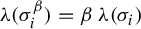
 with parallel faces and such that
$\unicode{x3bb} (\sigma _i^{\beta }) = \beta \, \unicode{x3bb} (\sigma _i)$
 . We denote by
$P_i$
 the centre of the cube
$\sigma _i$
 and let
$Q_i=\mathscr {P}(P_i)$
 ,
$i =1, \ldots ,N$
 . Since
$\|\mathscr {P}-\mathrm {Id}\|_{\infty } < \|\mathscr {P}-\mathrm {Id}\|_{\infty }+{\delta }/{3}$
 , applying Theorem 3.1 to the sets
$\{P_i\}_{i=1}^{N}$
 and
$\{Q_i\}_{i=1}^{N}$
 , we obtain a volume-preserving
$C^\infty $
 diffeomorphism of
$I^d$
 , F, equal to the identity on a neighbourhood of the boundary of
$I^d$
 and such that

Furthermore, since F sends a neighbourhood of
$P_i$
 by translation onto a neighbourhood of
$Q_i$
 , there exists
$0<\alpha <1$
 such that
$F=\mathscr {P}$
 on
$\sigma _i^{\alpha }$
 for every i. Consequently,
${\unicode{x3bb} \{x : \, \mathscr {P}(x) \neq F(x) \} \leq 1 - \alpha }$
 . If
$1-\alpha <\gamma $
 , the theorem is proved taking
$f=F$
 . Otherwise, it is clearly enough to obtain a map f which, in addition to satisfying the same conditions, coincides with
$\mathscr {P}$
 on the cubes
$\sigma _i^{\beta }$
 for some
$\beta $
 such that
$\beta>1-\gamma $
 . Fix
$\beta>1-\gamma $
 and define a map
$T \colon I^d \to I^d$
 (not volume-preserving) such that its restriction to each cube
$\sigma _i$
 is
$T^{\sigma _i,\alpha ,\beta }$
 , given by Lemma 4.1.
Finally, we define the map
$f:=T\circ F\circ T^{-1}$
 . This map satisfies the following points:
-
(i) $\unicode{x3bb} \{x \colon \mathscr {P}(x) \neq f(x) \} < \gamma $
, by construction; -
(ii) $x \in \bigcup _i \, \text {int}(\sigma _i^\beta )$
if and only if
$F(T^{-1}(x)) \in \bigcup _i \, \text {int} (\sigma _i^\alpha )$
; -
(iii) f is volume-preserving. In fact, by item (ii),
$$ \begin{align*} \det(J f(x))=\det(JT(F(T^{-1}(x))) \det(JF(T^{-1}(x))\det(JT^{-1}(x))=1, \end{align*} $$except in the boundary of $\sigma _i$
,
$\sigma _i^\alpha $
and
$\sigma _i^\beta $
.


It is clear that
$\|f-\mathrm {Id}\|_{\infty } \leq \|F-\mathrm {Id}\|_{\infty }+2 \|T-\mathrm {Id}\|_{\infty }<\|\mathscr {P}-\mathrm {Id}\|_\infty +\delta $
 .
As
$f=\mathrm {Id}$
 in
$\cup \sigma _i^\beta $
 , then
$\|f-\mathrm {Id}\|_p\leq \|f-\mathrm {Id}\|_{\infty }(1-\beta )^{{1}/{p}}<\delta $
 for
$\beta $
 large enough.
Using (2.1) and the fact that
$f=\mathrm {Id}$
 in
$\sigma _i^\beta $
 , we get

Notice that

To evaluate the norm of the partial derivatives of f, we start by noticing that:
-
• if $x\in \sigma _i$
, then
$T^{-1}(x)=T^{\sigma _i, \beta ,\alpha }(x)$
; -
• if $x\in \sigma _i\setminus \sigma _i^\beta $
, then
$T^{-1}(x)\in \sigma _i\setminus \sigma _i^\alpha $
and
$F(T^{-1}(x))\in \sigma _{i_1}\setminus \sigma _{i_1}^\alpha $
, where
$\sigma _{i_1}:=\mathscr {P}(\sigma _{i})$
. Then,
$f(x)=T^{\sigma _{i_1},\alpha ,\beta }(F(T^{-1}(x)))$
.






Using the chain rule, we have, for
$i,j=1,\ldots ,d$
 and almost every
$x\in I^d$
 ,

If
$x\in I_d\setminus \bigcup _i \sigma _i^\beta $
 , then, by the previous observations and (4.1), we have

and so,

Then, using (2.1), item (ii), the change of variables defined by
$T^{-1}$
 and the fact that
$F=\mathscr {P}$
 in
$\sigma ^\alpha _i$
 , we obtain

Hence, taking
$\beta $
 large enough, the conclusion follows.
We can now complete the proof of Theorem A.
Proof of Theorem A.
Let
$g \in \mathcal {G}_\unicode{x3bb} (I^d)$
 ,
$h\in \overline {\textrm {Lip}_\unicode{x3bb} (I^d)}^{\,p}$
 and consider
$\delta>0$
 . Let
$\mathcal {W}$
 be any weak topology neighbourhood of g. We will obtain
$f \in \textrm {Lip}_\unicode{x3bb} (I^d)$
 such that
$f \in \mathcal {W}$
 and

Recall that, if
$h\in \textrm {Lip}_\unicode{x3bb} (I^d)$
 , then
$\pi _1(h)=h$
 and
$\pi _2(h)=Dh$
 .
The proof will be divided into three steps.
Step 1. Assume first that
$h=\mathrm {Id}$
 . We only need to consider
$\mathcal {W}$
 of the form

Since the dyadic permutations are dense in
$\mathcal {G}_\unicode{x3bb} (I^d)$
 , the automorphism
$g\in \mathcal {G}_\unicode{x3bb} (I^d)$
 can be weakly arbitrarily approximated by a dyadic permutation R (see [Reference Alpern and Prasad3, Lemma 6.4]). Moreover, R can be weakly approximated by another dyadic permutation
$\mathscr {P}$
 satisfying

The technique for this approximation is described in the proof of [Reference Alpern and Prasad3, Theorem 6.2, p. 46].
Set
$\gamma _0:=\gamma - \unicode{x3bb} \{x : |g(x)-\mathscr {P}(x)| \geq \gamma \}$
 . Applying Theorem 4.2 (with
${\delta }/{2}$
 ) to the permutation
$\mathscr {P}$
 and using (4.2), we obtain a map
$f \in \textrm {Lip}_\unicode{x3bb} (I^d)$
 , with
$\|f-\mathrm {Id}\|_\infty < \|\mathscr {P}-\mathrm {Id}\|_\infty +{\delta }/{2}<\|g-\mathrm {Id}\|_\infty +\delta $
 ,
$\|D(f-\mathrm {Id})\|_p<{\delta }/{2}$
 and equal to the identity on a neighbourhood of the boundary, satisfying
$\unicode{x3bb} \{x \colon \mathscr {P}(x) \neq f(x) \} < \gamma _0$
 . From this last point, we also conclude that
$f \in \mathcal {W}$
 .
Step 2. Assume now that
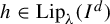
$h\in \textrm {Lip}_\unicode{x3bb} (I^d)$
 and consider
$\mathcal {W}$
 a weak topology neighbourhood of g in
$\mathcal {G}_\unicode{x3bb} (I^d)$
 .
As
$\mathcal {G}_\unicode{x3bb} (I^d)$
 , with the weak topology, is a topological group, then
$\mathcal {W}_h=\{\varphi \circ h^{-1}:\varphi \in \mathcal {W}\}$
 is a weak neighbourhood of
$g\circ h^{-1}$
 and

Using Step 1, consider
$f^*\in \textrm {Lip}_\unicode{x3bb} (I^d)$
 (which is in fact
$C^\infty $
 almost everywhere) such that
$f^*\in \mathcal {W}_h$
 and

for
$\delta ^*>0$
 to be defined later.
Consider
$f=f^*\circ h$
 . Notice that
$f\in \mathcal {W}$
 ,
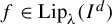
$f\in \textrm {Lip}_\unicode{x3bb} (I^d)$
 ,
$\|f-h\|_\infty =\|f^*-\mathrm {Id}\|_\infty $
 . However, using Lemma 2.6 and the hypothesis on
$f^*$
 , we have, for
$i,j=1,\ldots ,d$
 and
$M=\max _{i,j}\|{\partial h_i}/{\partial x_j}\|_\infty $
 ,

The conclusion follows choosing
$\delta ^*$
 conveniently.
Step 3. Suppose now that h is the limit of a sequence
$(h_n)_n$
 in
$\textrm {Lip}_\unicode{x3bb} (I^d)$
 . Let
$\delta ^*>0$
 , to be defined later, and
$n_0$
 such that
$\|\pi _1(h)-h_{n_0}\|_\infty ,\|\pi _2(h)-Dh_{n_0}\|_p< \delta ^*$
 .
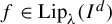
Applying Step 2, consider
$f\in \textrm {Lip}_\unicode{x3bb} (I^d)$
 such that
$f\in \mathcal {W}$
 and

Then, as
$\|\pi _1(h)-h_{n_0}\|_\infty <\delta ^*$
 ,

and, as
$\|\pi _2(h)-Dh_{n_0}\|_p < \delta ^*$
 , using (2.1),

and the conclusion follows if we choose
$\delta ^*=\min \{{\delta }/{3}, {\delta ^p}/{2}\}$
 .
Remark 4.3. The result of Theorem 4.2 and, consequently, of Theorem A is false if
$p\geq 1$
 . To see that, consider any permutation
$\mathscr {P}$
 different from the identity. Suppose that, for
$\delta ,\gamma>0$
 , there exists
$f\in \textrm {Lip}_\unicode{x3bb} (I^d)$
 , equal to the identity on a neighbourhood of the boundary of
$I^d$
 , satisfying

As
$f-\mathrm {Id}$
 equals to zero in the boundary of
$I^d$
 , then, using the Poincaré inequality, there exists C, depending on d and p, such that
$\|f-\mathrm {Id}\|_p \leq C\|D(f-\mathrm {Id})\|_p$
 . However,

which is a contradiction, as we can choose
$\delta ,\gamma $
 as small as we want.
5 Proof of Sobolev Oxtoby–Ulam theorem (Theorem B)
To prove the Sobolev Oxtoby–Ulam theorem, we need an auxiliary lemma that is the adaptation of [Reference Alpern and Prasad3, Lemma 7.2] to our setting. A crucial ingredient is our version of the Lusin theorem (Theorem A). As noticed before, the proof will be done in the cube
$I^d$
 . In brief terms, we will apply Lax’s approximation method, leveraging Hall’s marriage theorem to construct dyadic permutations that approximate volume-preserving homeomorphisms of the cube. While these permutations may initially decompose into multiple disjoint cycles, the fine scale of the cubes allows us to merge them into a single cycle by strategically reassigning a few cubes, all while preserving the closeness to the original homeomorphism.
Lemma 5.1. Let
$d\geq 2$
 ,
$0<p<1$
 and
$h\in \overline {\mathrm {Lip}_\unicode{x3bb} (I^d)}^{\,p}$
 . Then, given any
$\varepsilon>0$
 , there exists
$f\in \mathrm {Lip}_\unicode{x3bb} (I^d)$
 satisfying
$\|f-h\|_{1;\infty ,p}<\varepsilon $
 and such that, for some arbitrarily fine dyadic decomposition
$\{D_i\}_{i=1}^N$
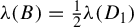
 , there is a compact set
$B\subset D_1$
 with
$\unicode{x3bb} (B)=\tfrac 12\unicode{x3bb} (D_1)$
 and
$f^i(B)$
 in the interior of the dyadic cube
$D_{i+1}$
 for
$i=0,\ldots , N-1$
 .
Proof. By [Reference Alpern and Prasad3, Theorem 3.3], there is a cyclic dyadic permutation
$\mathscr {P}$
 of some dyadic decomposition
$D_1,\ldots ,D_N$
 with
$\mathscr {P}(D_i)=D_{i+1}$
 , for
$i=1,\ldots ,N-1$
 and
$\mathscr {P}(D_N)=D_1$
 , with
$\|\mathscr {P}-\pi _1(h)\|_\infty <\varepsilon $
 . For
$D_i=\prod _{j=1}^d]a^i_j-\delta ,a^i_j+\delta [$
 , with
$\delta ={1}/({2\sqrt [d]{N}})$
 , define, for
$\alpha \in\ ]0,1[$
 ,
$D_{i,\alpha }=\prod _{j=1}^d]a^i_j-\alpha \delta ,a^i_j+\alpha \delta [$
 .
By Theorem A, there exists some
$f\in \textrm {Lip}_\unicode{x3bb} (I^d)$
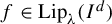 with
$\|f-h\|_{\infty ;1,p}<\varepsilon $
 , arbitrarily close to
$\mathscr {P}$
 in the weak topology. Therefore, there is a sequence
$(f_n)_n$
 in
$\textrm {Lip}_\unicode{x3bb} (I^d)$
 with
$\|f_n-h\|_{\infty ;1,p}<\varepsilon $
 , which converges to
$\mathscr {P}$
 in the weak topology.
In particular, for a, to be specified later, and
$\mu \in\ ]0,1[$
 satisfying
$\unicode{x3bb} (D_{1,\mu })>\tfrac 34\unicode{x3bb} (D_1)$
 , there exists
$n_0$
 such that
$\unicode{x3bb} (f_{n_0}(D_{i,\mu })\triangle \mathscr {P}(D_{i,\mu }))< a$
 for all
$i=1,\ldots ,N-1$
 . Note that, as
$\mathscr {P}(D_{i,\mu })=D_{i+1,\mu }$
 ,
$\unicode{x3bb} (f_{n_0}(D_{i,\mu })\setminus D_{i+1,\mu })< a$
 .
Let
$E_1=D_{1,\mu }$
 and, for each
$i>1$
 ,
$E_i=f(E_{i-1})\cap D_{i,\mu }$
 . By construction,
$E_i$
 is contained in the interior of
$D_i$
 ,
$\unicode{x3bb} (E_i)> \unicode{x3bb} (D_{1,\mu })-(i-1)a$
 and then, choosing
$a<{1}/({4(N-1)})$
 , we have
$\unicode{x3bb} (E_N)>\tfrac 12\unicode{x3bb} (D_1)$
 .
Consider
$B^*=(f^{N-1})^{-1}(E_N)$
 . Note that
$B^*$
 is a compact subset of
$D_1$
 and satisfies
$\unicode{x3bb} (B^*)>\tfrac 12\unicode{x3bb} (D_1)$
 , and
$f^i(B^*)$
 is included in
$D_{i+1,\mu }$
 .
Define
$g:[0,1[\rightarrow \mathbb {R}$
 by
$g(\alpha )=\unicode{x3bb} (B^*\cap D_{1,\alpha })$
 , which is a continuous function, since
$|g(\beta )-g(\alpha )|\leq |\unicode{x3bb} (D_{1,\beta })-\unicode{x3bb} (D_{1,\alpha })|=|(2\beta )^N-(2\alpha )^N|$
 for
$\alpha ,\beta \in ]0,1[$
 . In particular, there exists
$\alpha ^*$
 such that
$B=B^*\cap D_{1,\alpha ^*}$
 is a compact subset of
$D_1$
 , such that its measure is equal to
$\tfrac 12\unicode{x3bb} (D_1)$
 and
$f^i(B)$
 is included in the interior of
$D_{i+1}$
 for all
$i=0,\ldots ,N-1$
 .
Proof of Theorem B.
We exploit ideas developed in the proof of [Reference Alpern and Prasad3, Theorem 7.1], adapted with the many subtleties of the current Sobolev setting.
Let
$\mathcal {E}=\{f\in \mathcal {M}_\unicode{x3bb} (I^d):f \text {is ergodic}\}$
 and
$\mathcal {E}_\infty =\{f\in \mathcal {M}^{1,p}_\unicode{x3bb} (I^d): \pi _1(f) \text { is ergodic}\}$
 .
Consider
$(C_i)_{i\in \mathbb {N}}$
 an enumeration of all dyadic cubes of
$I^d$
 of all orders. For indices
$i,j$
 corresponding to dyadic cubes of the same order, define the subset
${\mathcal F}_{ij}$
 of
$\mathcal {M}_\unicode{x3bb} (I^d)$
 letting
$h\in {\mathcal F}_{ij}$
 if and only if there exists an h invariant set
$A\subseteq I^d$
 such that

In [Reference Alpern and Prasad3, Theorem 7.1], it was proved that
$\mathcal {M}_\unicode{x3bb} (I^d)\setminus \mathcal {E}=\bigcup _{i,j}\mathcal {F}_{ij}$
 and, for all
$i,j$
 ,
$\mathcal {F}_{ij}$
 is nowhere dense, that is,

The function f here is the one given by [Reference Alpern and Prasad3, Lemma 7.2], whose version in our context is Lemma 5.1.
Let
$\mathcal {G}_{ij}=\{h\in \mathcal {M}^{1,p}_\unicode{x3bb} (I^d):\pi _1(h)\in \mathcal {F}_{ij}\}$
 . It is clear that
$\mathcal {M}^{1,p}_\unicode{x3bb} (I^d)\setminus \mathcal {E_\infty }=\bigcup _{i,j}\mathcal {G}_{ij}$
 . To prove that
$\mathcal {G}_{ij}$
 is nowhere dense, consider
$h\in \mathcal {G}_{ij}$
 and
$\varepsilon>0$
 . Using Lemma 5.1 and the above, there exists
$f\in \textrm {Lip}_\unicode{x3bb} (I^d)$
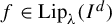 and
$\delta>0$
 such that

If
$g\in \mathcal {M}^{1,p}_\unicode{x3bb} (I^d)$
 and
$\|g-f\|_{1;\infty ,p}<\delta $
 then, by (2.5),
$\|\pi _1(g)-f\|_\infty <\delta $
 . So, as
$B^\infty (f,\delta )\cap \mathcal {F}_{ij}=\emptyset $
 , we conclude that
$\pi _1(g)\not \in \mathcal {F}_{ij}$
 , that is,
$g\not \in \mathcal {G}_{ij}$
 .
6 Proof of genericity of topological transitivity (Theorem C)
Our proof of Theorem C will be done in the cube
$I^d$
 and follows the same steps as [Reference Alpern and Prasad3, Theorem 4.1] using as a novelty our Theorem 3.1, where we deal with a finer topology.
Since, in this section,
$p\geq 1$
 , an element
$f\in \mathcal {M}^{1,p}_\unicode{x3bb} (I^d)$
 is identified with
$\pi _1(f)$
 , which is a volume-preserving homeomorphism admitting weak partial derivatives in
$L^p(I^d)$
 .
Proof of Theorem C.
Let
$\mathcal {Y}$
 be the (enumerable) set of the open dyadic cubes of any size and consider, for
$A,B\in \mathcal {Y}$
 ,

If we denote by
$\mathcal {T}$
 the set of all topologically transitive elements of
$\mathcal {M}^{1,p}_\unicode{x3bb} (I^d)$
 , then, as any open set in
$I^d$
 contains a dyadic cube,

As for
$A,B\in \mathcal {Y}$
 ,
$\mathcal {T}_{A,B}$
 is open (as it is open in the uniform topology), we are left to show that it is also a dense subset of
$\mathcal {M}_\unicode{x3bb} (I^d)$
 . To do this, it is enough to consider any
$f\in \textrm {Lip}_\unicode{x3bb} (I^d)$
 and
$\varepsilon>0$
 , and find
$g\in \mathcal {T}_{A,B}\cap \textrm {Lip}_\unicode{x3bb} (I^d)$
 such that

By [Reference Alpern and Prasad3, Theorem 3.3], there exists a cyclic dyadic permutation
$\mathscr {P}$
 of some dyadic decomposition
$D_1,\ldots ,D_N$
 , with
$\mathscr {P}(D_k)=D_{k+1}$
 , for
$k=1,\ldots ,N-1$
 and
${\mathscr {P}(D_N)=D_1}$
 , with
$\|f-\mathscr {P}\|_\infty <\varepsilon /2$
 . We can also suppose that the size of these dyadic cubes is less than the sizes of A and B. Let
$c_k$
 stand for the centre of
$D_k$
 .
We now apply Theorem 3.1 to the sets
$ \{f(c_k)\}_{k=1}^N$
 and
$\{\mathscr {P}(c_k)\}_{k=1}^N$
 , obtaining a
$C^{\infty }$
 volume-preserving diffeomorphism F of
$I^d$
 which is equal to the identity in a neighbourhood of the boundary of
$I^d$
 , sends by translation a ball centred in
$f(c_k)$
 onto the ball centred in
$\mathscr {P}(c_k)$
 and, for
$\delta =\delta (\varepsilon )$
 to be defined later,

Since
$f\in \textrm {Lip}_\unicode{x3bb} (I^d)$
 and F is a
$C^\infty $
 volume-preserving diffeomorphism, we get
$g:= F\circ f\in \textrm {Lip}_\unicode{x3bb} (I^d)$
 . Moreover, for all
$k=1,\ldots ,N-1$
 ,

Let
$i,j$
 be such that
$c_i\in A$
 and
$c_j\in B$
 . Then, as g permutes in a cyclical way the points
$c_1,\ldots ,c_N$
 , there exists
$n\in \mathbb {N}$
 such that
$g^n(c_i)=c_j$
 and then
$g^n(A)\cap B\not =\emptyset $
 . Hence,
$g\in \mathcal {T}_{A,B}$
 .
It is clear that
$\|g-f\|_\infty =\|F\circ f-f\|_\infty =\|F-I_d\|_\infty <\varepsilon $
 .
Finally, to estimate the norm of the partial derivatives of
$g-f$
 , we use the chain rule given by Lemma 2.6. We get, for a certain
$N>0$
 depending on
$\|Df\|_\infty $
 ,
$\|D(g-f)\|_p\leq N\,\|D(F-I)\|_p<N\delta \leq \varepsilon $
 if
$\delta ={\varepsilon }/{N}$
 .
7 Construction of an example
Now, we are in a condition to exhibit
$(g,h)\in \mathcal {M}^{1,p}_\unicode{x3bb} (I^d)$
 for
$0<p<1$
 such that h is not the weak derivative of g, proving that
$\mathcal {M}^{1,p}_\unicode{x3bb} (I^d)$
 is not a function space.
For
$d\geq 2$
 , we will give an example of a sequence
$(f_n)_n$
 of measure-preserving Lipschitz homeomorphisms of
$I^d$
 converging uniformly to the identity Id and such that the sequence
$(Df_n)_n$
 converges in
$L^p(I^d)^{d^2}$
 , with
$0<p<1$
 , to
$DJ$
 , where
$J:I^d\rightarrow I^d$
 is defined by
$J(x_1,x_2,x_3,\ldots ,x_d)=(1-x_1,1-x_2,x_3,\ldots ,x_d)$
 .
It is enough to prove that, for all
$\delta>0$
 , there exists f, a measure-preserving Lipschitz homeomorphisms of
$I^d$
 , such that

It is clear that if we have such an f for
$d=2$
 , then
$\tilde {f}$
 defined as

defines the intended function.
So, let us consider
$d=2$
 . Given
$\delta>0$
 , consider a dyadic partition of
$I^2$
 such that the
$\sigma _i$
 squares of the partition have diameter less than
$\delta $
 . Define
$F:[0,1]^2\rightarrow [0,1]^2$
 such that, in each square
$\sigma _i$
 of the partition, F is given by the restriction to
$\sigma _i$
 of the function G given by Lemma 3.7 for
$d=2$
 , A the centre of
$\sigma _i$
 and
$s=\frac 12\unicode{x3bb} (\sigma _i)^{\frac 12}$
 .
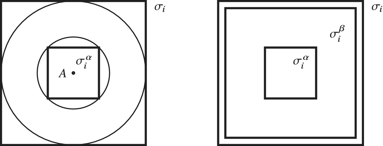
Consider a square
$\sigma _i^\alpha $
 inscribed in the circle centred in A and radius
${s}/{2}$
 .
For
$\alpha \leq \beta \leq 1$
 , let
$T_\beta :[0,1]^2\rightarrow [0,1]^2$
 be a homeomorphism such that, in each
$\sigma _i$
 ,
$T^\beta $
 is, as in Lemma 4.1, a dilatation from
$\sigma _i^\alpha $
 to
$\sigma _i^\beta $
 (see Figure 2). Finally, consider
$f=T_\beta \circ F\circ T^{-1}_\beta $
 .
An illustration of the example.

As
$f(\sigma _i)=\sigma _i$
 , then
$\|f-\mathrm {Id}\|_\infty <\delta $
 .
In what concerns the derivative, as f is a rotation of an angle of
$\pi $
 in each
$\sigma _i^\beta $
 , then, using (2.1),

Following the last part of the proof of Theorem 4.2, we get the estimates

Choosing
$\beta <1$
 large enough, we obtain
$\|{\partial f_i}/{\partial {x_j}}-{\partial J_i}/{\partial {x_j}}\|_p<\delta $
 .
To prove that f is measure-preserving, we will show that for all i and almost every
$x\in \sigma _i$
 ,
$|\!\det Df(x)|=1$
 . In fact, for such x, we have, as F is measure-preserving,

and the conclusion follows, using Lemma 4.1 noticing that
$T^{-1}_\beta (x)\in \sigma _i^\alpha $
 if and only if
$F(T^{-1}_\beta (x))\in \sigma _i^\alpha $
 .
Acknowledgements
We are deeply grateful to the anonymous referees for their insightful and constructive comments, which significantly improved the clarity, rigour and overall quality of this manuscript. A.A., D.A. and M.J.T. were partially financed by Portuguese Funds through FCT (Fundação para a Ciência e a Tecnologia) through the research Project UID/00013/2025 (https://doi.org/10.54499/UID/00013/2025). M.B. was partially financed by Portuguese Funds through FCT (Fundação para a Ciência e a Tecnologia) within the project: UID/04561/2025 (https://doi.org/10.54499/UID/04561/2025).