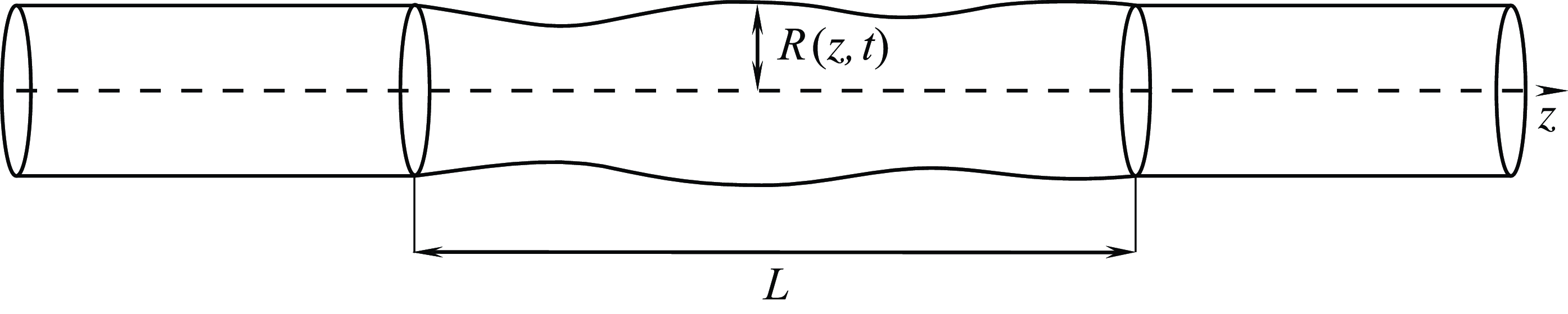
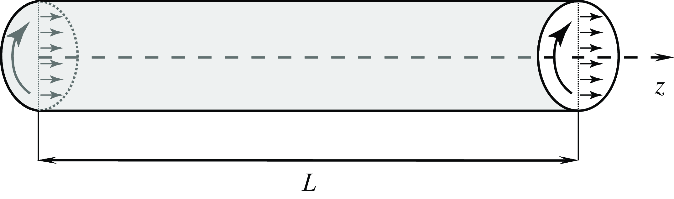
1. Introduction
Many fluid flows that play important roles in technical and natural processes occupy spatial domains elongated in one direction: flows in pipes, channels and flumes, film flows, boundary layers, jets, etc. To study the stability of such flows, it is often assumed that the domain is infinitely long, and a special class of perturbations in the form of travelling waves
 $\sim \textrm{e}^{{i}(kx-\omega t)}$
is analysed. However, infinitely long flows do not exist in reality, whereas the relation between the stability of infinitely long and finite-length flows turns out to be tricky. An instructive example is provided by rotating inviscid flow in a pipe studied by Wang & Rusak (Reference Wang and Rusak1996): if the rotation speed is sufficiently large, then the flow in a long finite-length pipe is always unstable, while that in an infinitely long pipe is neutrally stable. Plane Poiseuille flow serves as an opposite example: it is unstable for supercritical Reynolds numbers in the infinitely long channel, but a finite-length (no matter how long!) channel makes the flow stable.
The drastic difference between infinitely long and finite-length systems is caused by domain boundaries in the finite-length case: a single travelling wave cannot satisfy the boundary conditions, thus cannot exist in the bounded domain; instead, wave reflection from the boundaries takes place. That is why in finite-length systems, instead of travelling waves, eigenmodes of the form
 $\sim A(x)\,\textrm{e}^{{-i}\omega t}$
drive the stability properties, where
 $A(x)$
must satisfy the boundary conditions.
However, despite the disappointing examples showing defectiveness of infinitely long theoretical models of real finite-length flows, there exists a general framework for treating long finite-length problems, which is known as global instability theory. Namely, in spatially one-dimensional systems of large but finite domain, the complex eigenfrequency spectrum is concentrated around a specific asymptotic curve in the complex plane, and this curve is determined by the dispersion relation of an infinitely long system, as proved by Kulikovskii (Reference Kulikovskii1966a
); see also Pitaevskii & Lifshitz (Reference Pitaevskii and Lifshitz1981, § 65). If part of such a curve lies in the upper half-plane of the complex
 $\omega$
plane, then a system of sufficiently long length is unstable; such instability is called global. Recall that the instability condition of an arbitrarily long but finite system in general differs from the instability condition of an infinitely long system.
Note that some confusion exists in terminology: ‘global instability’ is attributed to spatially homogeneous finite-length systems (Kulikovskii Reference Kulikovskii1966a ), as well as to spatially developing infinitely long systems (Le Dizés et al. Reference Le Dizés, Huerre, Chomaz and Monkewitz1996). Although both approaches can be united, because turning points in spatially developing flows can be considered as effective boundary conditions that reflect and refract incident waves (Kulikovskii Reference Kulikovskii1985), the mathematical apparatus used in both theories is different. To be specific, in this study we consider ‘global instability’ in the first sense, i.e. in the context of homogeneous finite-length systems.
Global instability in finite-length problems has been studied in physical systems of a very different nature: Poiseuille flows in a pipe of finite length (Kulikovskii Reference Kulikovskii1966b , Reference Kulikovskii1968; Aizin & Maksimov Reference Aizin and Maksimov1978), thermocapillary convection (Priede & Gerbeth Reference Priede and Gerbeth1997), jet flows of a liquid (Shugai & Yakubenko Reference Shugai and Yakubenko1997; Yakubenko Reference Yakubenko1997), plasma instability (Kulikovskii Reference Kulikovskii1970), elastic plates in a flow of an incompressible fluid (Peake Reference Peake2004), supersonic panel flutter (Vedeneev Reference Vedeneev2016), spiral waves (Echebarria, Hakim & Henry Reference Echebarria, Hakim and Henry2006), flames (Nichols, Chomaz & Schmid Reference Nichols, Chomaz and Schmid2009), and axisymmetric Couette flows of a magnetic fluid (Priede & Gerbeth Reference Priede and Gerbeth2009). Similar analysis has also been used in the studies of thermoplasticity models (Kameniarzh Reference Kameniarzh1972), vibrations of fluid-conveying pipes (Kulikovskii & Shikina Reference Kulikovskii and Shikina1988; Doaré & de Langre Reference Doaré and de Langre2002), flows over cavities (Tuerke et al. Reference Tuerke, Sciamarella, Pastur, Lusseyran and Artana2015), and other problems (Doaré & de Langre Reference Doaré and de Langre2006).
Kulikovskii (Reference Kulikovskii1966a
) obtained the equation of the curve, which serves as an attractor of eigenvalues for large system lengths, only partially, by considering its uppermost sections in the complex
 $\omega$
plane, which correspond to the fastest growing modes. This is sufficient to obtain the stability criterion, but in many cases, e.g. to control the instability, it is also important to know how the instability modes are generated, through the analysis of the eigenfrequency loci and interactions in the complex plane prior to the transition to instability. To this end, in this work, the equation of the asymptotic curve is generalised to the case of arbitrary eigenfrequencies, which is discussed in § 2. In § 3, we analyse possible local topologies of this curve, and show that only three types of topology are stable with respect to small changes of the problem parameters. Bifurcations of the curve topology are analysed in § 4. A special consideration is necessary for the imaginary
 $\omega$
axis, which is discussed in § 5. In § 6, we demonstrate theoretical results of this work on three examples: supersonic panel flutter, flutter of a soft fluid-conveying pipe, and the stability of rotating pipe flow. Finally, in § 7 we summarise the results of this study.
2. Frequency equation for a one-dimensional system of large length
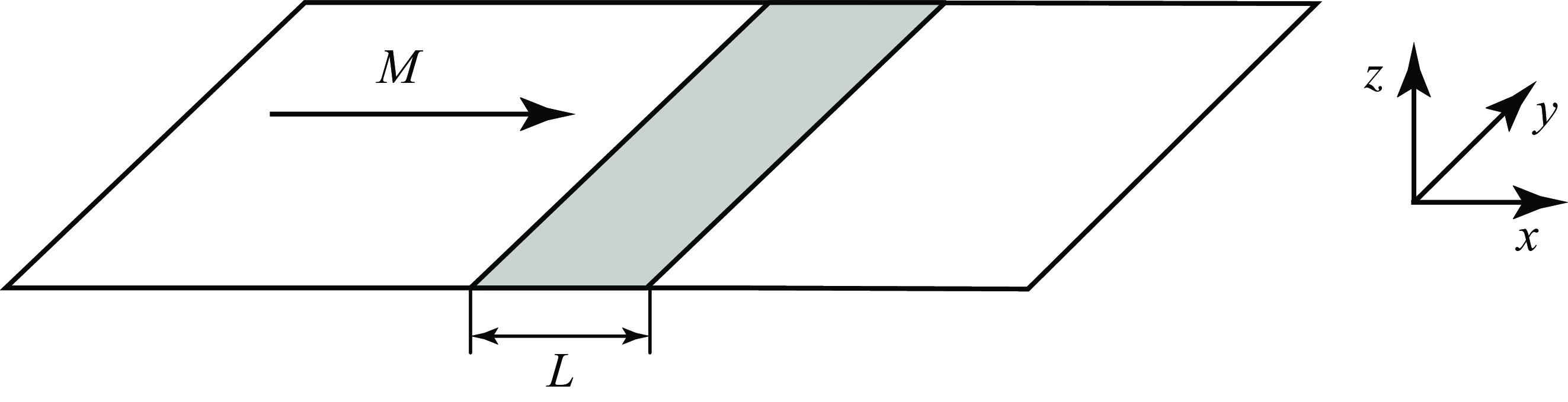
Consider a spatially one-dimensional homogeneous system, in which we are interested in the eigenfrequency spectrum. The system length is
 $L$
, so boundary conditions are assigned at
 $x=\pm L/2$
. At this point, we do not specify the physical nature of the problem; one may assume, say, plates or shells in an axial flow (either external of internal).
2.1. General properties of the dispersion relation for an infinite-length problem
First, let us consider the general properties of solutions of the dispersion equation of an infinitely long system
 \begin{equation} \mathcal {D}(k,\omega )=0, \end{equation}
where
 $k$
and
 $\omega$
are the complex wavenumber and frequency of travelling wave
 $\sim \textrm{e}^{{i}(kx-\omega t)}$
. We will assume that the system satisfies the causality principle, that is, there is a finite value
 $P=\max \limits _{k\in \mathbb {R},{1\leqslant j\leqslant M}} {\textrm {Im}}\,\omega _j(k)$
, where
 $M$
is the number of eigenfrequencies
 $\omega _j(k)$
. This condition means that travelling waves with real wavenumbers cannot grow arbitrarily fast. If this condition is not satisfied, then a smooth solution to the Cauchy problem does not exist (the system blows up), which means that the mathematical problem is not well-posed. In this case, the mathematical formulation of the physical problem must be updated to exclude infinitely fast growing perturbations. As a rule, unlimited growth, if it occurs, takes place as
 $k\to \infty$
; in this case, the mathematical formulation of the problem must be modified to take into account the damping mechanisms of short-wave disturbances.
Under this condition, for
 ${\textrm {Im}}\,\omega \gt P$
, all solutions
 $k_j=k_j(\omega )$
of the dispersion relation are complex. Let us number the roots of the dispersion equation
 $k=k(\omega )$
in descending order of the imaginary part for large
 ${\textrm {Im}}\,\omega$
, and let us divide them into two groups:
 ${\textrm {Im}}\, k_j\gt 0$
,
 $j=1,\ldots ,s$
, and
 ${\textrm {Im}}\, k_j\lt 0$
,
 $j=s+1,\ldots ,N$
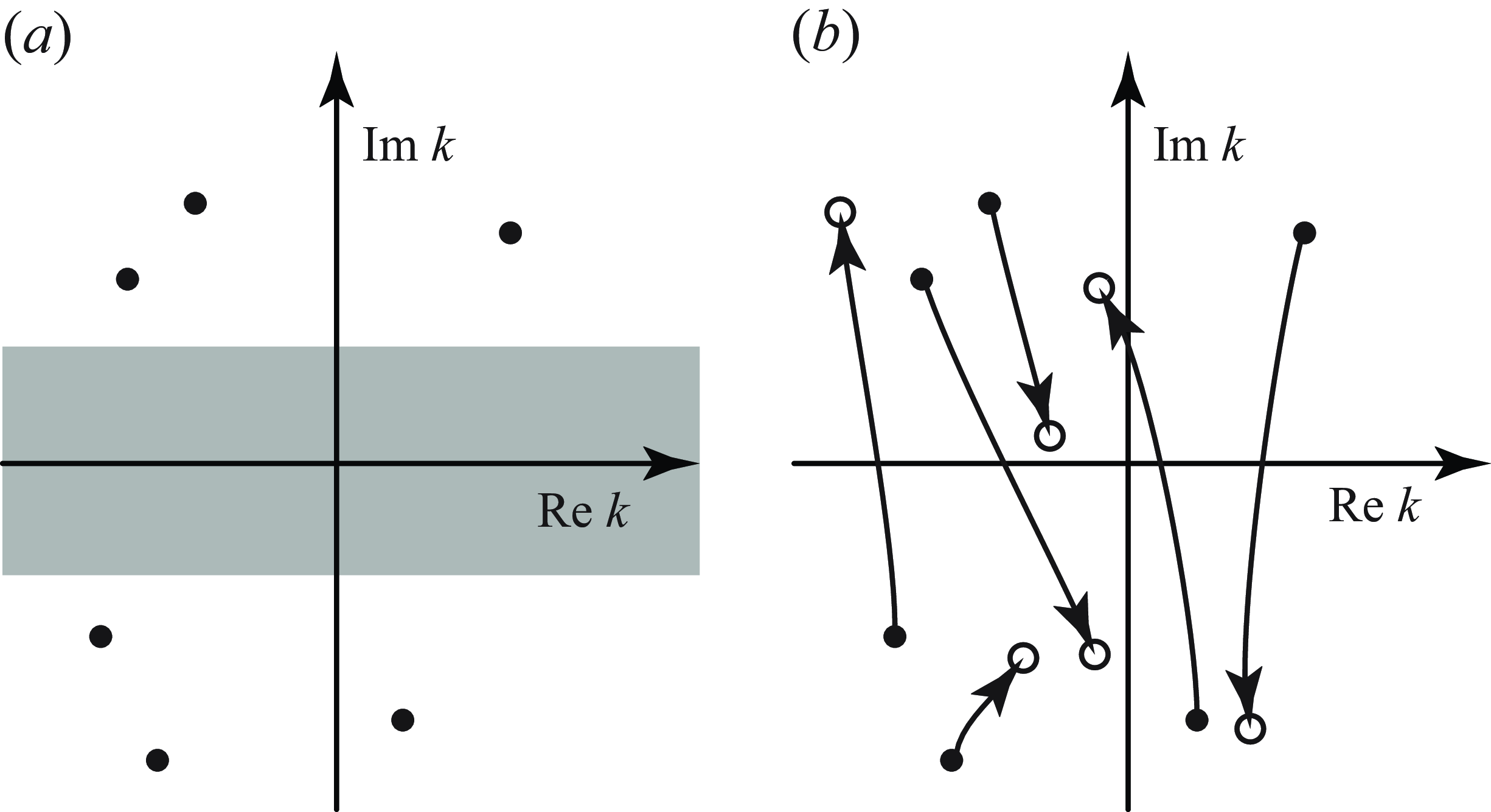
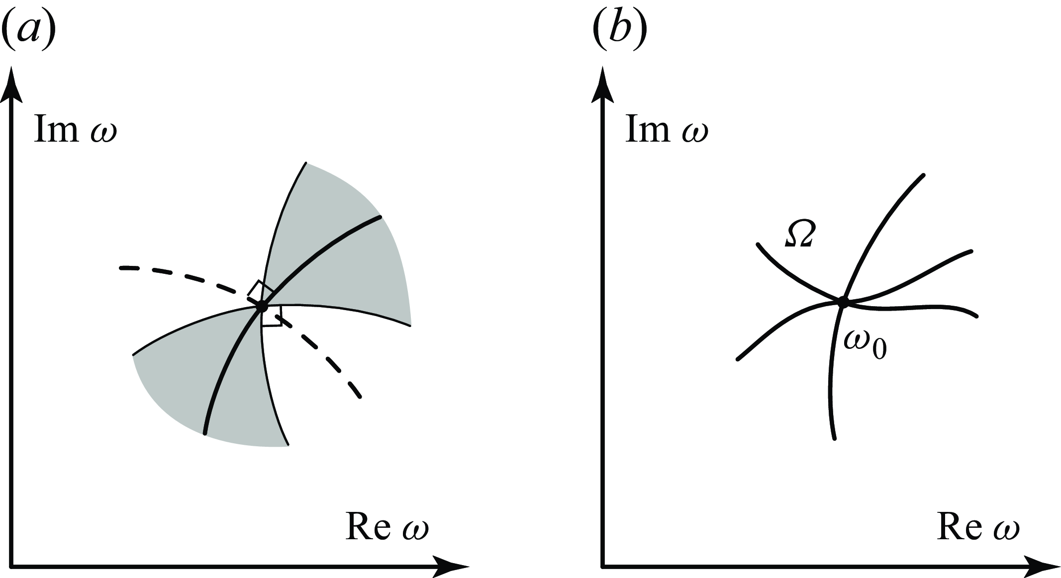
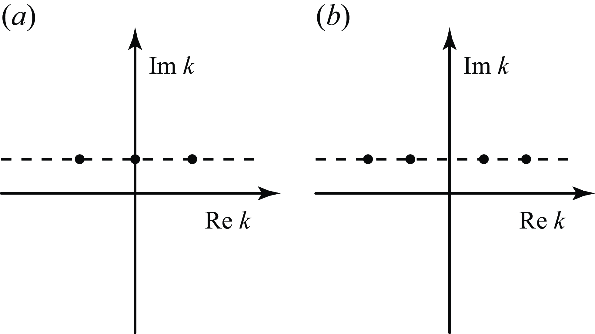
(figure 1
a). Waves corresponding to wavenumbers from the first group are right-travelling, and those from the second group are left-travelling (see § 2.3 of Briggs Reference Briggs1964; Ashpis & Reshotko Reference Ashpis and Reshotko1990). Then the criterion of the well-posedness of the boundary value problem can be formulated as follows (Hersh Reference Hersh1964): the number of boundary conditions at each boundary of the system
 $x=\pm L/2$
must be equal to the number of waves travelling away from that boundary, that is,
 $s$
conditions at the left-hand end (
 $x=-L/2$
), and
 $N-s$
conditions at the right-hand end (
 $x=L/2$
) must be specified. This ensures unambiguous amplitudes of reflected waves produced by waves incident to each boundary.
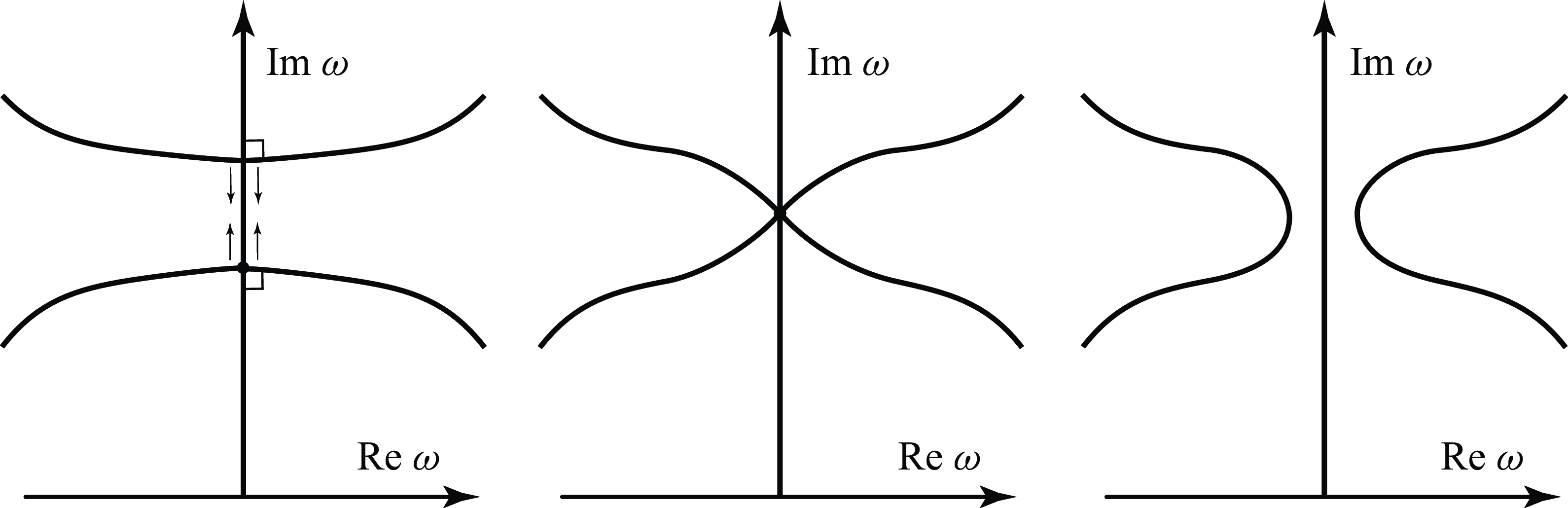
Location of wavenumbers
 $k(\omega )$
in the complex plane for
 ${\textrm {Im}}\,\omega \gt P$
: (a) right- and left-travelling waves are well separated by the shaded region; (b) their loci as
 ${\textrm {Im}}\,\omega$
decreases.

When lowering
 ${\textrm {Im}}\,\omega$
, the wavenumbers move in their complex plane and ‘mix’ with each other, as shown schematically in figure 1(b). As a result, for arbitrary values of
 $\omega$
, it is not possible to distinguish left- and right-travelling waves, and the only way to do that is to increase
 ${\textrm {Im}}\,\omega$
and track the sign of
 ${\textrm {Im}}\, k(\omega )$
. To give a physical interpretation, consider a travelling wave produced by a harmonic point source oscillating with a real frequency
 $\omega$
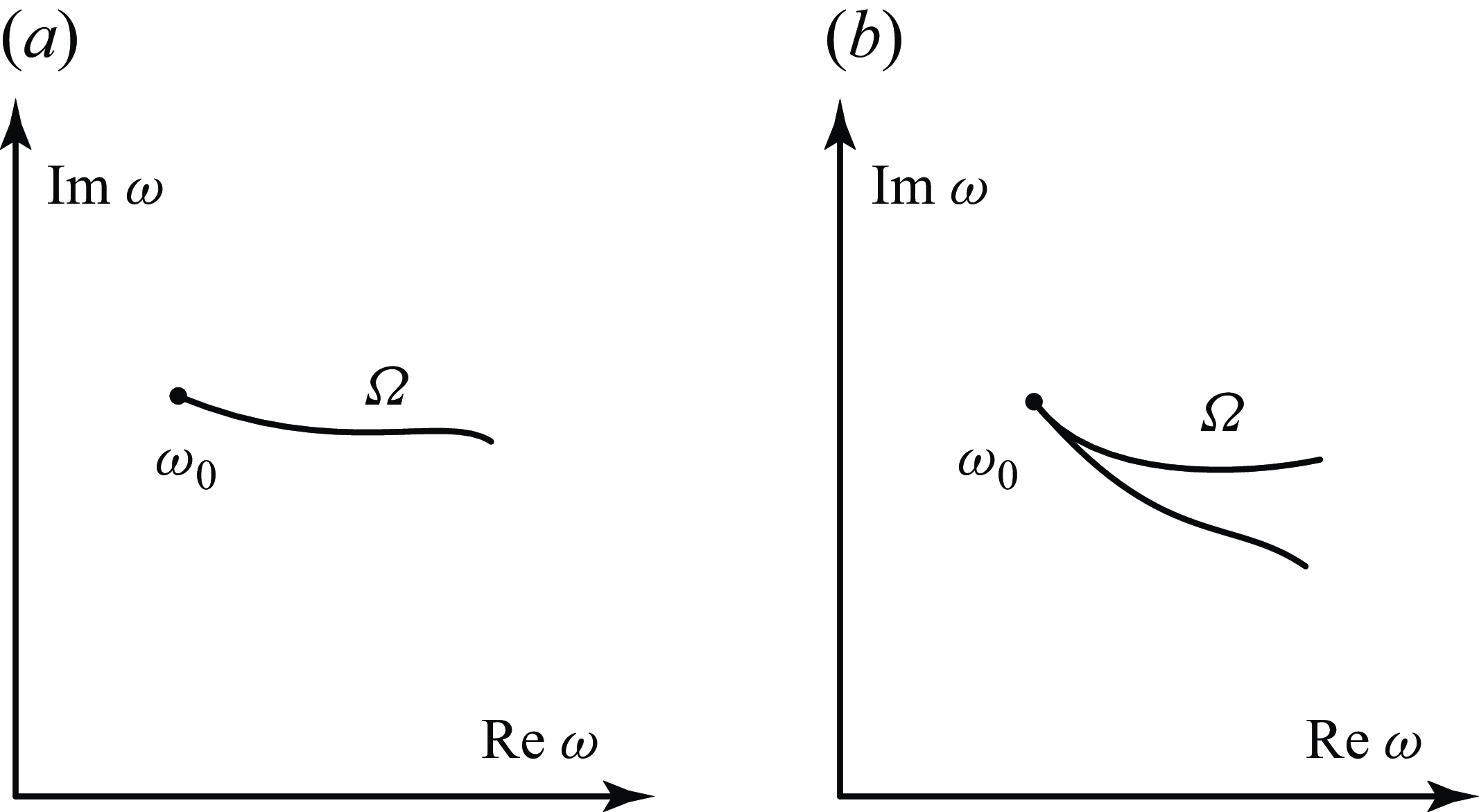
(figure 2
a). Let the wave be spatially amplifying in the positive
 $x$
-direction (i.e.
 ${\textrm {Im}}\, k(\omega ) \lt 0$
), which can signify that it is either a left-travelling damped wave, or a right-travelling amplified wave. Note that neither phase nor group speed can provide information about the direction of the wave motion. Increasing
 ${\textrm {Im}}\,\omega$
means adding temporal amplification to the source. Regardless of spatial amplification (or damping)
 ${\textrm {Im}}\, k$
at the real frequency, it will be dominated by sufficiently large
 ${\textrm {Im}}\,\omega$
so that the wave will become spatially damped when moving away from the source, and the wave direction will be clear through the sign of
 ${\textrm {Im}}\, k$
(figure 2
b).
(a) Waves produced by a harmonic point source with a real frequency; distinction between right-travelling amplified and left-travelling damped waves is not possible. (b) The same waves produced by a temporarily amplified point source: right- and left-travelling waves are well distinguished by the sign of
 ${\textrm {Im}}\, k$
.

2.2. Frequency equation for a finite-length problem
To search for eigenmodes of the finite-length problem, we consider a linear combination of
 $N$
travelling waves
 \begin{equation} \sum _{m=1}^N C_m\, \textrm{e}^{{i}(k_m(\omega )\,x-\omega t)}, \end{equation}
which is substituted into
 $N$
boundary conditions, which leads to a linear algebraic system of equations for the amplitudes
 $C_m$
. From the condition for the existence of a non-zero solution, we obtain the frequency equation

where
 $a_{ij}=a_{ij}(k_j(\omega ),\omega )$
are coefficients determined by boundary conditions. The eigenfrequencies of a finite-length system are the solutions of this equation. Note that the first
 $s$
lines in the determinant have terms with exponent
 $\textrm{e}^{{-i}k_j L}$
, while the remaining
 $(N-s)$
lines have
 $\textrm{e}^{{i}k_j L}$
, where
 $s$
is equal to the number of boundary conditions specified on the left-hand end, which, in turn, is determined by the number of waves moving to the right from this end at large
 ${\textrm {Im}}\,\omega$
.
2.3.
Frequency equation form for the case of large
 $L$

Let us assume that the length of the system is sufficiently large, i.e.
 $L\gg 1$
. For any given
 $\omega$
, let us sort the wavenumbers in descending order of the imaginary part
 ${\textrm {Im}}\, k_j(\omega )$
:
 \begin{equation} {\textrm {Im}}\, k_1(\omega )\geqslant {\textrm {Im}}\, k_2(\omega )\geqslant \ldots\geqslant {\textrm {Im}}\, k_s(\omega )\geqslant {\textrm {Im}}\, k_{s+1}(\omega )\geqslant \ldots \geqslant {\textrm {Im}}\, k_N (\omega ). \end{equation}
This sorting is natural for
 ${\textrm {Im}}\,\omega \gt P$
as explained in § 2.1, but now we use it for any
 $\omega$
. Then for
 $L\to \infty$
, the leading term of the determinant (2.3) is the product of the exponential factor
 \begin{equation} \textrm{e}^{-{i}(k_1(\omega )+\cdots +k_{s-1}(\omega )+k_s(\omega )-k_{s+1}(\omega )-k_{s+2} (\omega )-\cdots -k_{N}(\omega ))L/2} \end{equation}
and two minors of the matrix
 $A$
, composed of the coefficients
 $a_{ij}$
: one has order
 $s$
and occupies the upper left corner, the other is of order
 $N-s$
and occupies the lower right corner of this matrix. The next highest term is the product of the exponential factor
 \begin{equation} \textrm{e}^{-{i}(k_1(\omega )+\cdots +k_{s-1}(\omega )-k_s(\omega )+k_{s+1}(\omega )-k_{s+2} (\omega )-\cdots -k_{N}(\omega ))L/2}, \end{equation}
where the signs of
 $k_s$
and
 $k_{s+1}$
are reversed, and its coefficient is the product of the same minors of the matrix obtained from
 $A$
by permutation of the
 $s$
th and
 $(s+1)$
th columns. Thus keeping the two main terms in (2.3), and cancelling by the exponent (2.5), we obtain the leading-order form of (2.3) as
 $L\to \infty$
:
 \begin{equation} |A_s|\,|A_{N-s}|+|A_s'|\,|A_{N-s}'|\,\textrm{e}^{{i}(k_s(\omega )-k_{s+1}(\omega ))L}=0. \end{equation}
We now proceed to the analysis of solutions of (2.7) for
 $L\gg 1$
. Since
 $L$
is present only in the exponential factor, three cases are possible.
-
(i) If
${\textrm {Im}}\, k_s(\omega )\not ={\textrm {Im}}\, k_{s+1}(\omega )$
for a given frequency
$\omega$
, then as
$L\to \infty$
, the second term becomes negligible so that (2.7) yields(2.8)If the roots
\begin{equation} |A_s(\omega )||A_{N-s}(\omega )|=0 . \end{equation}
$k_1,\ldots, k_s$
for a given value of
$\omega$
correspond to right-travelling waves (i.e. these are the same branches of wavenumber as for
${\textrm {Im}}\,\omega \to +\infty$
), then the roots of this equation are called ‘one-sided frequencies’ (Kulikovskii Reference Kulikovskii1966a
). Indeed, if we consider a semi-infinite system in which
$x\in [-L/2,+\infty )$
, and assume the decaying condition as
$x\to +\infty$
, then in a linear combination of waves (2.2), it is necessary to retain only
$s$
right-travelling waves. Their substitution into the
$s$
boundary conditions at
$x=-L/2$
gives the frequency equation(2.9)Similarly, the natural frequencies of a semi-infinite system in which
\begin{equation} |A_s(\omega )|=0. \end{equation}
$x\in (-\infty,L/2]$
are given by the frequency equation(2.10)Thus for a system that is finite in both directions, the spectrum of one-sided frequencies (2.8) is the union of the frequency spectra of two semi-infinite systems, which explains the name of this part of the spectrum. If one of these frequencies has a positive imaginary part, then the system is unstable; in this case, the instability is also called one-sided.
\begin{equation} |A_{N-s}(\omega )|=0. \end{equation}
-
(ii) Next, assume that (2.8) is satisfied, but the roots
$k_1,\ldots, k_s$
(or
$k_{s+1},\ldots, k_N$
, depending on which multiplier in (2.8) is zero) include both right- and left-travelling waves. This is possible due to ‘mixing’ of wavenumbers at small
${\textrm {Im}}\,\omega$
, as discussed in § 2.1. We will call such frequencies ‘anomalous one-sided’. They are not truly one-sided frequencies, because in the semi-infinite problem, only waves moving in one direction are present. Although the existence of such frequencies is in general possible, it seems counterintuitive, and the authors are not aware of any physical system where such eigenfrequencies exist. -
(iii) If (2.8) is not satisfied, then as
$L\to \infty$
, the first and second terms in (2.7) must be balanced to cancel each other, which yields(2.11)Equation (2.11) defines the curve
\begin{equation} {\textrm {Im}}\,k_s(\omega )={\textrm {Im}}\, k_{s+1}(\omega ). \end{equation}
$\Omega$
on the complex plane
$\omega$
, which has the following property: for large values of
$L$
in the vicinity of any of its points, there is always a frequency that satisfies (2.7), and vice versa, any such frequency that is not one-sided lies in the vicinity of this curve. Thus eigenfrequencies that are not one-sided, although they form a discrete set, are located near the curve
$\Omega$
, more closely and densely concentrating around the curve, the greater the length of the system
$L$
. In other words,
$\Omega$
attracts eigenfrequencies as
$L\to \infty$
. If a piece of
$\Omega$
is located in the upper half-plane
$\omega$
, then the frequencies located near this piece correspond to growing disturbances. The spectrum defined by (2.11), and the instability caused by this spectrum, are called global (Kulikovskii Reference Kulikovskii1966a
).


Thus for sufficiently large
 $L$
, the frequency spectrum is separated into a regular one-sided, anomalous one-sided and global spectra. The larger
 $L$
, the higher the accuracy of such a separation, namely, the more accurate the transition from (2.3) to (2.7) and then to (2.8) and (2.11).
It is worth mentioning that the one-sided spectrum essentially depends on the boundary conditions, because the matrices in (2.8) consist of
 $a_{ij}$
that come from the boundary conditions. On the contrary, (2.11) does not depend on the particular boundary conditions, which govern the particular distribution of the eigenfrequencies along the
 $\Omega$
curve, but not the curve itself.
Note that in the case of polynomial coefficients
 $a_{ij}(\omega )$
, the one-sided spectrum is always finite (and often absent), while the global frequencies usually form a countable set. Therefore, in this study, we will limit ourselves to the analysis of the configuration of the global spectrum.
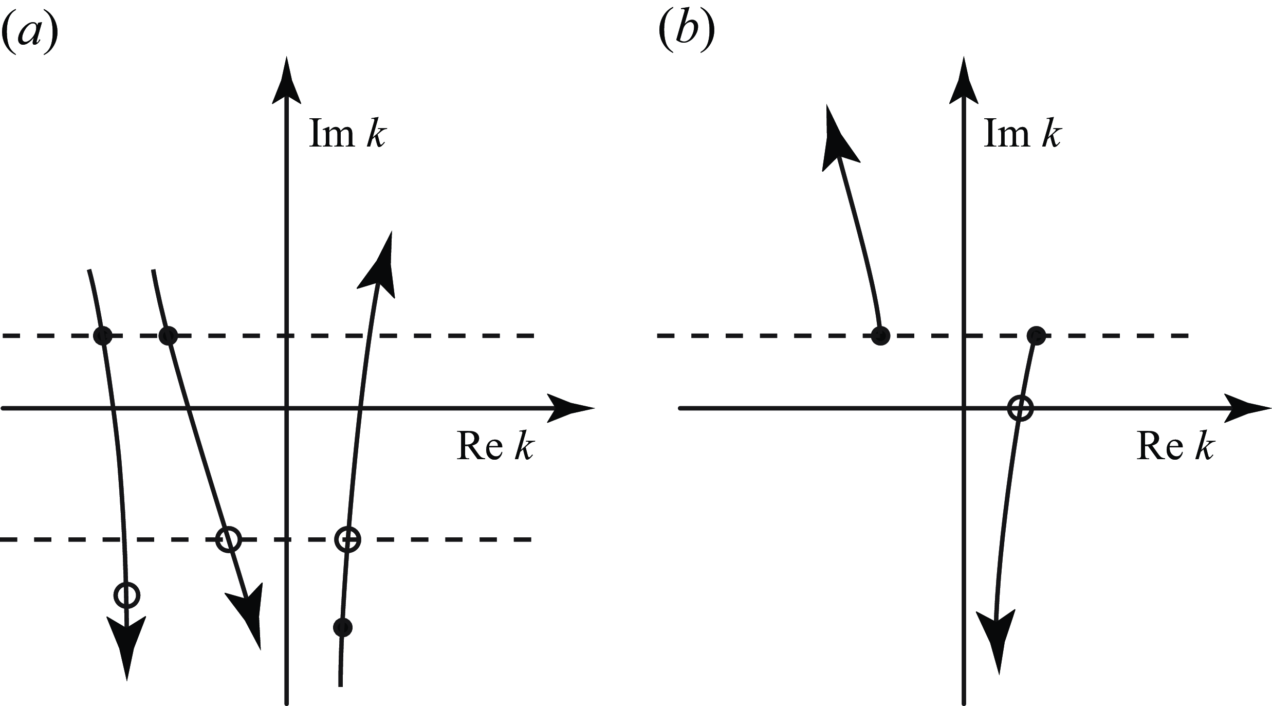
(a) Proof of the fastest growing global mode formation by the waves travelling in opposite directions. (b) Proof of the instability of the infinite-length system following from the global instability of the finite-length system. Arrows show the wavenumber loci with increasing
 ${\textrm {Im}}\,\omega$
; empty circles correspond to larger
 ${\textrm {Im}}\,\omega$
than filled circles.

2.4. Properties of the global spectrum
We have proved that all frequencies of the global spectrum are located near the curve (2.11). Let us now prove the converse statement: near every point of this curve, there exist global frequencies, if
 $L$
is sufficiently large. Indeed, consider a point
 $\omega _0$
satisfying (2.11), and nearby located points
 $\omega =\omega _0+\Delta \omega$
. Assume that the Taylor expansion
 \begin{equation} k_s-k_{s+1}=a+b\,\Delta \omega +o(\omega ),\quad a\in \mathbb {R}, \end{equation}
is valid. Solving the frequency equation (2.7), we find
 \begin{align} i(k_s-k_{s+1})=ia+ib\,\Delta \omega =\frac {1}{L}\ln \left (-\frac {|A_s|\,|A_{N-s}|}{|A_s'|\,|A_{N-s}'|}\right ) +\frac {2\unicode{x03C0} n i}{L},\quad n\in \mathbb {Z}. \end{align}
Taking real and imaginary parts of this equality, and denoting
 $b=b_r+ib_i$
,
 $\Delta \omega =\Delta \omega _r+i\,\Delta \omega _i$
, we get
 \begin{align} b_i\,\Delta \omega _r+b_r\,\Delta \omega _i=-\frac {1}{L}\ln \left (-\frac {|A_s|\,|A_{N-s}|}{|A_s'|\,|A_{N-s}'|}\right ), \end{align}
 \begin{align} b_r\,\Delta \omega _r-b_i\,\Delta \omega _i=\frac {2\unicode{x03C0} n}{L}-a. \end{align}
Note that one should select such
 $n$
that provide
 $2\unicode{x03C0} n /L\approx a$
to ensure the expansion (2.12). The determinant of this system is non-zero, so there are solutions
 $\Delta \omega$
such that
 $\Delta \omega \to 0$
as
 $L\to \infty$
. Thus we have proved that each point of the
 $\Omega$
curve attracts discrete eigenfrequencies of the boundary value problem as
 $L\to \infty$
.
Next, let us prove that the most unstable global eigenfrequencies are located near sections of
 $\Omega$
in which the roots
 $k_s$
,
 $k_{s+1}$
correspond to waves moving in opposite directions. Indeed, if
 ${\textrm {Im}}\, k_s(\omega )={\textrm {Im}}\, k_{s+1}(\omega )$
, but the branches
 $ k_{s,s+1}(\omega )$
are not the same as for
 ${\textrm {Im}}\,\omega \gt P$
(as shown in figure 3(a) by filled circles), then increasing
 ${\textrm {Im}}\,\omega$
will necessarily result in motion of wavenumbers to their ‘native’ half-planes where they are located for
 ${\textrm {Im}}\,\omega \gt P$
. Among several possible equalities
 ${\textrm {Im}}\, k_s(\omega )={\textrm {Im}}\, k_{s+1}(\omega )$
, the last one (i.e. at the largest possible
 ${\textrm {Im}}\,\omega$
) will occur for the branches
 $ k_{s,s+1}(\omega )$
from different groups (figure 3(a), empty circles). However, this statement is in general not correct for arbitrary points of
 $\Omega$
: due to possible redistribution of the order of
 ${\textrm {Im}}\, k_j$
at small
 ${\textrm {Im}}\,\omega$
, the equality
 ${\textrm {Im}}\, k_s(\omega )={\textrm {Im}}\, k_{s+1}(\omega )$
can correspond to the waves moving in the same direction, as shown in figure 3(a) by filled circles.
Now let us prove that if the finite-length problem is globally unstable (i.e. there exist points of the
 $\Omega$
curve with
 ${\textrm {Im}}\,\omega \gt 0$
), then the infinitely long problem is necessarily unstable. Consider two wavenumbers
 $k_{s,s+1}$
with equal imaginary parts (figure 3
b) corresponding to the largest
 ${\textrm {Im}}\,\omega _{\textit{fin}}$
. Since they move to opposite half-planes as
 ${\textrm {Im}}\,\omega$
increases, one of them necessarily crosses the real
 $k$
axis. This means that there exist
 $k\in \mathbb {R}$
with
 ${\textrm {Im}}\,\omega (k)\geqslant {\textrm {Im}}\,\omega _{\textit{fin}}\gt 0$
, i.e. there is a growing travelling wave, which finalises the proof. Note that the maximum growth rate of the infinite-length problem turns out to be not less than the maximum global growth rate of the finite-length problem.
A converse statement is in general incorrect: instability of the infinite-length problem does not necessarily mean global instability of the finite-length problem. However, if the instability of the infinite-length problem is absolute, then the finite-length problem is globally unstable. This becomes evident if one notes that the absolute instability frequency, i.e. saddle point of the
 $\omega (k)$
function, at which
 ${\rm d}\omega /{\rm d}k=0$
, corresponds to the branch point of the inverse function
 $k(\omega )$
, at which
 $k_s=k_{s+1}$
. Moreover, if the
 $\omega (k)$
saddle point is the absolute instability frequency, then the branches
 $k_{s,s+1}$
correspond to waves travelling in opposite directions. Of course, at such points, the equality (2.11) is also satisfied, i.e. they belong to the
 $\Omega$
curve. In § 3 we will show that such points are dead ends of the
 $\Omega$
curve.
We stress that the global instability curve only represents a limit state of the global spectrum as
 $L\to \infty$
. For small and moderate lengths
 $L$
, the location of eigenfrequencies in the complex plane is governed by the full frequency equation (2.3) and can be arbitrarily far from the
 $\Omega$
curve. In particular, instability of finite-length system is possible when the infinite-length system is stable. However, since the global instability is impossible for a stable infinite-length system, sufficiently long systems will always become stable.
The latter has one important exception: neutral global stability. In this case, we can only guarantee that the growth rate in the finite-length system is
 ${\textrm {Im}}\,\omega _{\textit{fin}}\to 0$
as
 $L\to \infty$
, but we cannot guarantee that the growth rate is not positive. Such a seemingly contradicting example is provided by the rotating pipe flow problem mentioned in § 1: a finite-length problem of arbitrarily large length is unstable, whereas an infinitely long problem is stable. In that problem, the infinite problem is stable only neutrally; the finite-length problem is also globally neutrally stable. Consequently, finite-length problem eigenfrequencies have
 ${\textrm {Im}}\,\omega \approx 0$
. But it turns out that while the growth rate
 ${\textrm {Im}}\,\omega$
tends to zero as
 $L\to \infty$
, its sign stays positive. This case will be considered in § 6 in more detail.
2.5. Physical interpretation
The derivation of the equation for the global instability asymptotic curve (2.11) was performed in an abstract mathematical manner. To provide a more intuitive insight into the structure of global modes, consider waves moving in the system.
Let us imagine that at the left-hand end of the system,
 $x=-L/2$
, we excite a disturbance in the form of
 $s$
right-travelling waves:
 \begin{align} \sum _{j=1}^{s}C_{\!j} \textrm{e}^{{i}(k_j x-\omega t)}. \end{align}
When they reach the right-hand end,
 $x=L/2$
, the amplitude of one of the waves, namely the
 $s$
th wave, significantly exceeds the amplitudes of the remaining waves, since the wavenumbers
 $k_j$
are numbered in descending order of the imaginary part, which means that the
 $s$
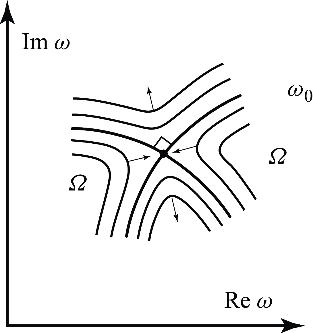
th wave has the largest spatial growth rate or the smallest spatial decay rate among right-travelling waves (figure 4
a). Therefore, the remaining waves can be ignored at the reflection process from the right-hand end. After the reflection of the
 $s$
th wave,
 $N-s$
reflected left-travelling waves leave the right-hand end. For similar reasons, the amplitudes of all waves, except for the
 $(s+1)$
th one, can be neglected when they arrive at the left-hand end
 $x=-L/2$
(figure 4
b).
Thus for large
 $L$
, the dominant role in the reflection process is played by two waves running in opposite directions: the
 $s$
th and
 $(s+1)$
th waves.
Hierarchy of (a) right-travelling and (b) left-travelling waves. Arrows show the directions of the waves’ motion.

Let us calculate the amplitudes of these waves at different moments in time. When the wave
 $C_s \textrm{e}^{{i}(k_sx-\omega t)}$
, excited at the left-hand end, reaches the right-hand end, its amplitude is equal to
 $C_s\textrm{e}^{-{\textrm {Im}}\, k_sL/2}$
(the factor
 $\textrm{e}^{{-i}\omega t}$
can be ignored, since it is the same for all waves). After reflection, it will turn into the wave
 $A_{s (s+1)}C_s \textrm{e}^{-{\textrm {Im}}\, k_sL/2}\,\textrm{e}^{{\textrm {Im}}\, k_{s+1}L/2}\,\textrm{e}^{{i}(k_{s+1}x-\omega t)}$
, where
 $A_{s (s+1)}$
is the reflection coefficient of the
 $s$
th wave into the
 $(s+1)$
th wave at the right-hand end. When the latter wave reaches the left-hand end, its amplitude will be equal to
 $A_{s (s+1)}C_s \textrm{e}^{-{\textrm {Im}}\, k_sL/2}\,\textrm{e}^{{\textrm {Im}}\, k_{s+1}L}$
. After reflection from the left-hand end, it will turn into the wave
 $A_{(s+1)s}A_{s (s+1)}C_s \textrm{e}^{-{\textrm {Im}}\, k_sL/2}\,\textrm{e}^{{\textrm {Im}}\, k_{s+1}L}\,\textrm{e}^{-{\textrm {Im}}\, k_sL/2}\,\textrm{e}^{{i}(k_sx-\omega t)}$
, where
 $A_{(s+1)s}$
is the reflection coefficient of the
 $(s+1)$
th wave into the
 $s$
th wave at
 $x=-L/2$
. Consequently, after two reflections, we obtain the originally excited wave, but in general of different phase and amplitude.
In the case when the amplitude and phase of the
 $s$
th wave after two reflections coincide with the initial ones, the described process will be repeated cyclically in a self-sustained manner, i.e. it will represent an eigenmode. The coincidence condition has the form
 \begin{equation} A_{(s+1)s}A_{s (s+1)}\,\textrm{e}^{{\textrm {Im}} (k_{s+1}-k_s) L}=1. \end{equation}
For large
 $L$
, it can be satisfied only if
 ${\textrm {Im}}\, k_s(\omega )\approx {\textrm {Im}}\, k_{s+1}(\omega )$
, that is, for
 $\omega$
, lying in the neighbourhood of the curve (2.11). On the other hand, in the neighbourhood of any point determined by (2.11), one can find a frequency that satisfies (2.17).
Physically, the reflection coefficients that are determined by the boundary conditions become unimportant for large
 $L$
, because the amplitude of every wave is governed mostly by its exponential spatial growth rate accumulated over the long domain. The initial amplitudes at each end that depend on the reflection coefficients can be dominated by the spatial growth by just a slight change in the frequency. That is why the eigenfrequencies in the long domain become insensitive to the boundary conditions, yielding the global spectrum limit. The condition (2.11) means that the spatial growth rate of a left-travelling wave and spatial decay rate of a right-travelling wave (or vice versa) coincide, which provides an almost unaltered amplitude of the doubly reflected wave. Small variation of the frequency near the one satisfying (2.11) provides fine tuning of the amplitude and phase to get truly original waves and organise a self-sustained reflection process.
Summarising, we conclude that global eigenmodes have form of a superposition of two most amplified (or least damped) waves moving in opposite directions, while at the ends of the system, they transform into each other.
3. Local topology of the asymptotic
$\Omega$
curve

Let us investigate possible local configurations of the curve
 $\Omega$
, which is determined, as established above, by the system
 \begin{equation} {\textrm {Im}}\, k_1(\omega )\geqslant {\textrm {Im}}\, k_2(\omega )\geqslant \ldots\geqslant {\textrm {Im}}\, k_s(\omega )= {\textrm {Im}}\, k_{s+1}(\omega )\geqslant \ldots \geqslant {\textrm {Im}}\, k_N( \omega ). \end{equation}
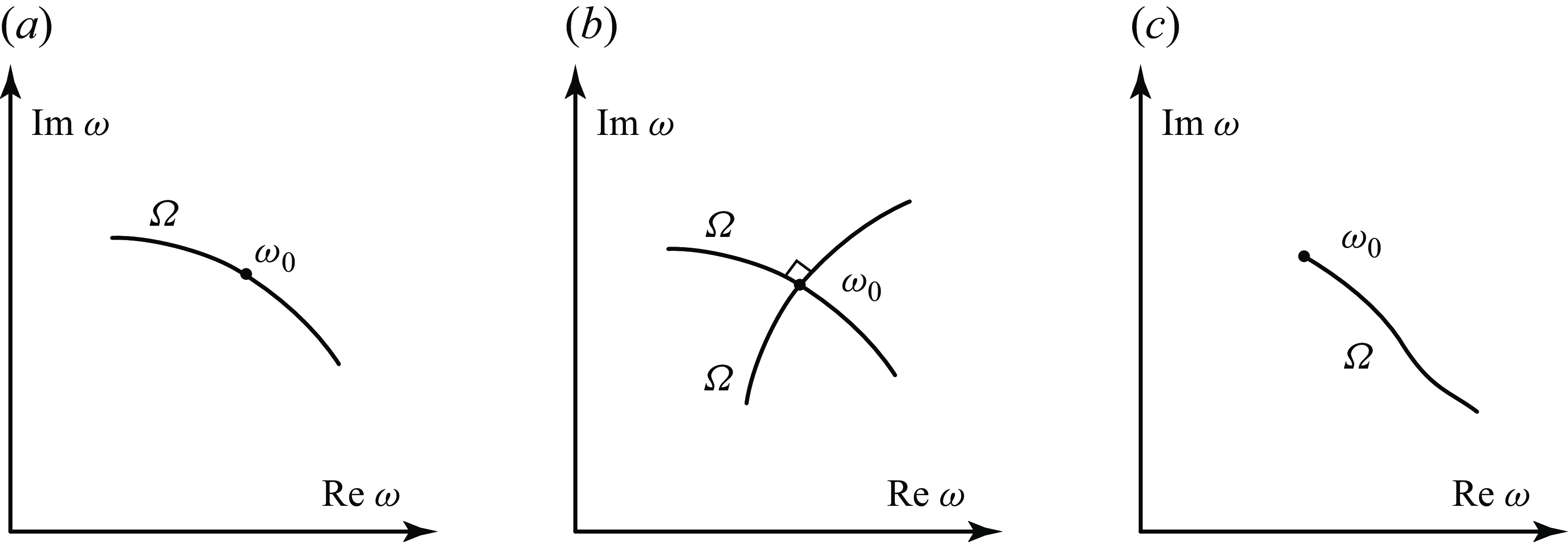
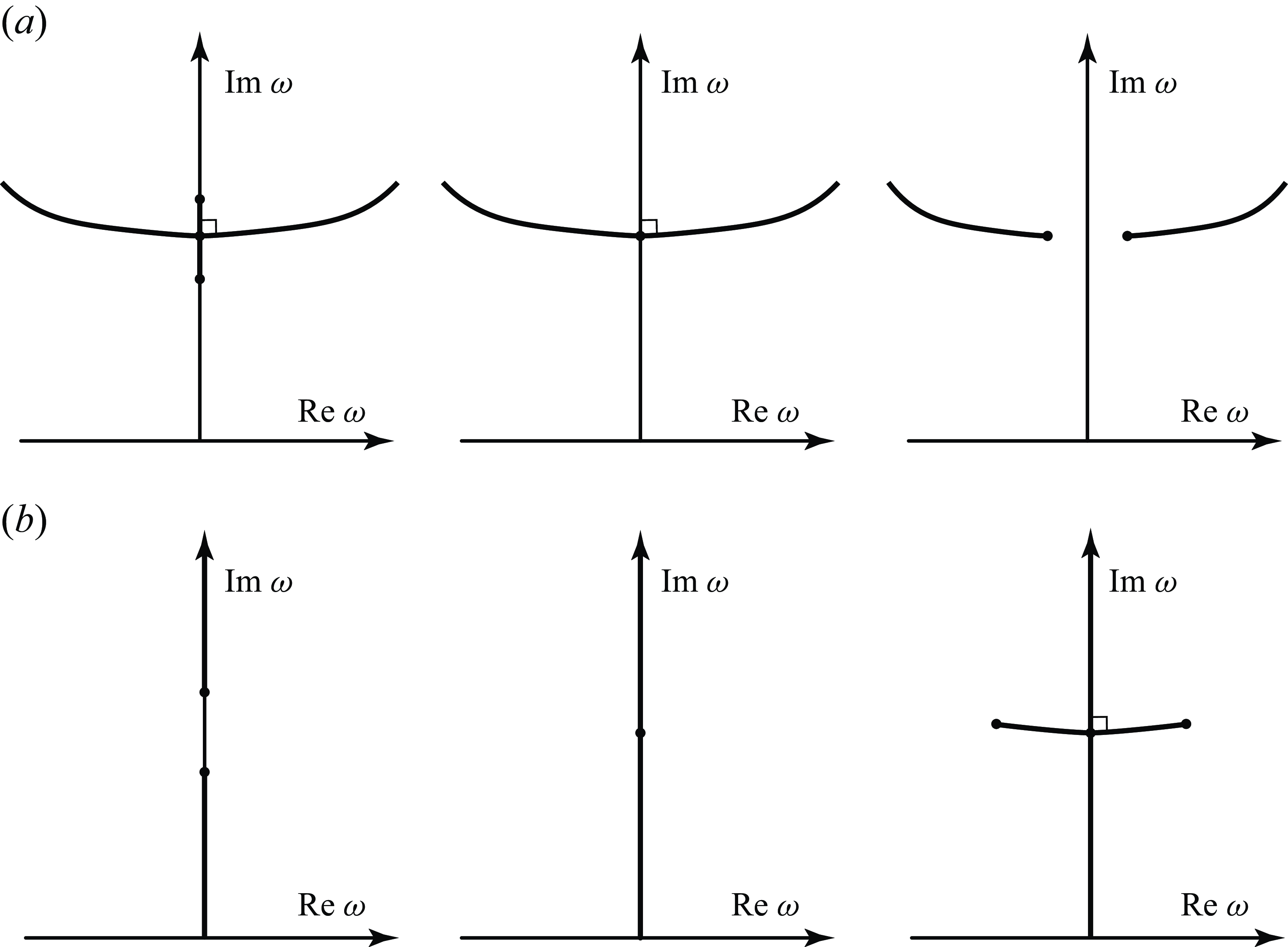
Local structure of curve
 $\Omega$
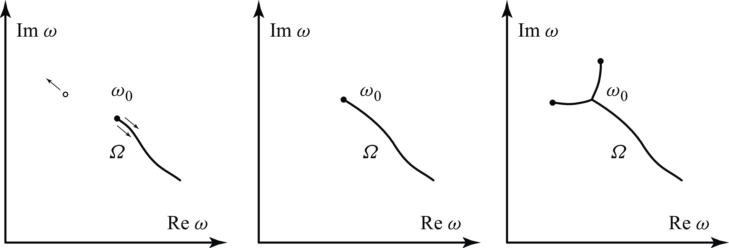
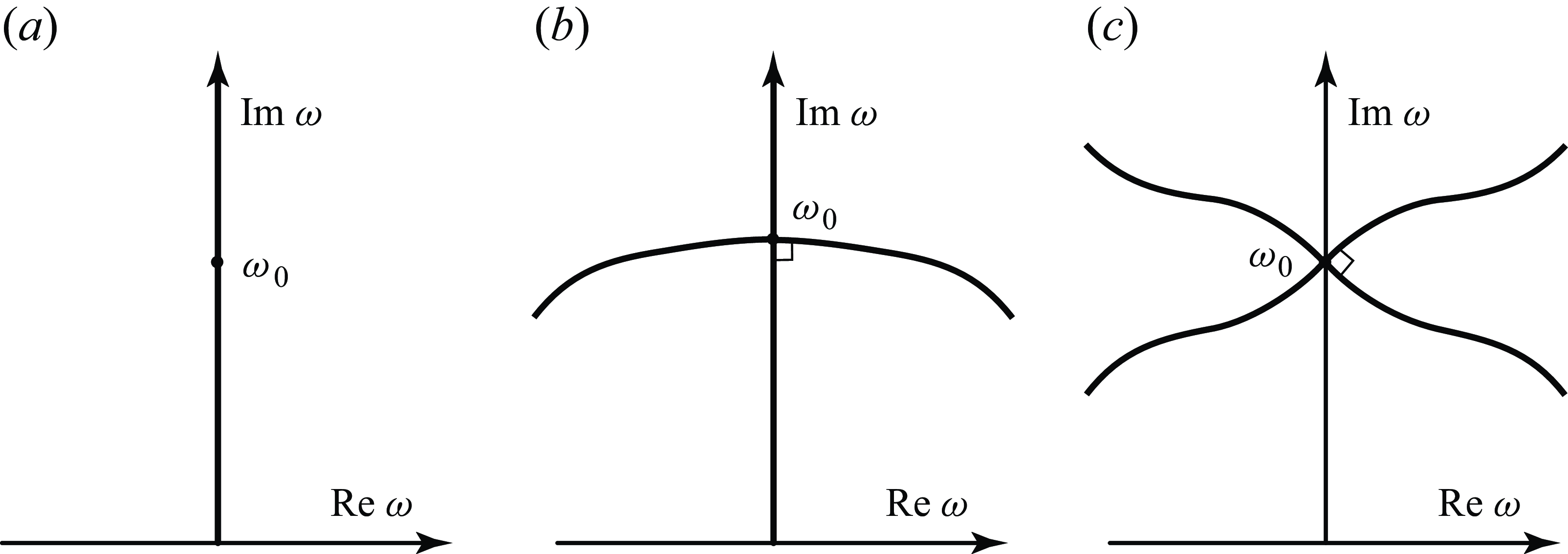
: (a) case 1a, regular point; (b) case 1b, intersection of two curves at angle
 $\unicode{x03C0} /2$
; (c) case 2, branch point
 $k(\omega )$
, dead end of the curve.

Let there be a point
 $\omega _0$
at the curve. Let us analyse which points
 $\omega$
close to
 $\omega _0$
also belong to the curve. Consider several possible cases.
-
1. Let the roots
$k_s$
,
$k_{s+1}$
at the point
$\omega _0$
have equal imaginary parts, and let the imaginary parts of
$k_{s-1}(\omega )$
and
$k_{s+2}$
be different. In addition, let the point
$\omega _0$
not be a branch point of
$k_s$
,
$k_{s+1}$
. Then the following Taylor expansions are valid:(3.2)where the expansion coefficients
\begin{align} &k_s(\omega )=k_s(\omega _0)+a_1(\omega -\omega _0)+a_2(\omega -\omega _0)^2+\cdots , \nonumber \\ &k_{s+1}(\omega )=k_{s+1}(\omega _0)+b_1(\omega -\omega _0)+b_2(\omega -\omega _0)^2+\cdots , \end{align}
$a_j$
and
$b_j$
,
$j=1, 2, \ldots$
, are functions of
$\omega _0$
.-
(a) If
$a_1(\omega _0)\not = b_1(\omega _0)$
, then the equality
${\textrm {Im}}\, k_s(\omega )={\textrm {Im}}\, k_{s+1}$
, up to linear terms, reduces to the equation of the straight line
${\textrm {Im}} ( (a_1-b_1)(\omega -\omega _0))=0$
. Such points
$\omega _0$
are regular points of the curve
$\Omega$
; the curve passes through them without any bifurcations (figure 5
a). -
(b) If
$a_1(\omega _0) = b_1(\omega _0) \Leftrightarrow {\rm d}k_s/{\rm d}\omega ={\rm d}k_{s+1}/{\rm d}\omega$
, but
$a_2(\omega _0) \not = b_2(\omega _0)$
, then, up to quadratic terms, we obtain
${\textrm {Im}} ((a_2-b_2)(\omega -\omega _0)^2)=0$
. Let us denote
$\omega -\omega _0=w\, \textrm{e}^{{i}\varphi }$
,
$a_2-b_2=A\,\textrm{e}^{{i}\alpha }$
. Then the equation can be rewritten as(3.3)Here,
\begin{equation} Aw^2\, \textrm{e}^{{i}(2\varphi +\alpha )}=q\,\textrm{e}^{i\unicode{x03C0} m} \quad \Rightarrow \quad 2\varphi +\alpha =\unicode{x03C0} m \quad \Rightarrow \quad \varphi =\frac {\unicode{x03C0} m}{2}-\frac {\alpha }{2}. \end{equation}
$A$
and
$\alpha$
are the known modulus and argument of
$a_2-b_2$
,
$w$
and
$\varphi$
are the unknown modulus and argument of the
$\omega$
increment,
$q$
is an arbitrary non-negative number, and
$m\in \mathbb {N}$
. Thus the equation of the curve gives four directions with angle
$\unicode{x03C0} /2$
between them. Locally at a given point, the curve represents the intersection of two straight lines with angle
$\unicode{x03C0} /2$
(figure 5
b). Note that the presence of such points on the curve is a special situation, since the equation
${\rm d}k_s/{\rm d}\omega ={\rm d}k_{s+1}/{\rm d}\omega$
has a finite number of roots, and the passage of the curve
$\Omega$
through such roots is, generally speaking, an exceptional situation.
-
(c) At points where a larger number of derivatives coincide,
${\rm d}^jk_s/{\rm d}\omega ^j={\rm d}^jk_{s+1}/{\rm d}\omega ^j$
,
$j=1,\ldots p$
, locally the curve
$\Omega$
has the form of the intersection of
$j+1$
straight lines with angles
$\unicode{x03C0} /(p+1)$
between adjacent rays. The existence of such points is an extremely rare situation and is not considered here in more detail.
-
-
2. As before, let the roots
$k_s$
,
$k_{s+1}$
at the point
$\omega _0$
have equal imaginary parts, and the imaginary parts
$k_{s-1}(\omega )$
and
$k_{s +2}$
are different from them. But now the point
$\omega _0$
is the branch point of
$k_s$
,
$k_{s+1}$
. Then the following expansions are valid:(3.4)where the ellipsis denotes the regular part of the expansion. Let us denote
\begin{equation} k_{s,s+1}(\omega )=k(\omega _0)\pm a\sqrt {\omega -\omega _0}+\cdots , \end{equation}
$a=A\,\textrm{e}^{{i}\alpha }$
. Then the equation of the curve
$\Omega$
gives(3.5)As can be seen, there is a unique direction for the continuation of the
\begin{align} {\textrm {Im}} (a\sqrt {\omega -\omega _0})=0 \quad & \Rightarrow \quad {\textrm {Im}} (A\sqrt {w}\, \textrm{e}^{{i}(\alpha +\varphi /2)})=0 \quad \Rightarrow \quad \alpha +\varphi /2=\unicode{x03C0} m \nonumber \\ & \Rightarrow \quad \varphi =-2\alpha -2\unicode{x03C0} m. \end{align}
$\Omega$
curve from the point
$\omega _0$
; thus the branch points
$k_{s,s+1}$
are the dead ends of
$\Omega$
(figure 5
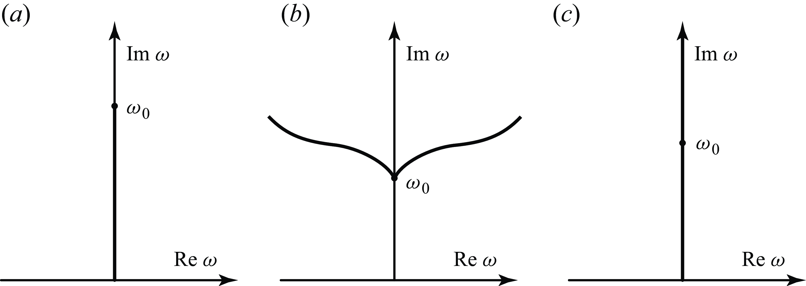
c).
It is well known that the branch point of the
$k(\omega )$
function corresponds to a saddle point of the reverse function
$\omega (k)$
, which is associated with absolute instability of an infinitely long system, if in this point
${\textrm {Im}}\,\omega \gt 0$
. Consequently, any configuration of the curve
$\Omega$
, which partially occupies the upper half-plane, but dead ends, if any, lie in the bottom half-plane, corresponds to the global instability of a finite-length system, which is not accompanied by absolute instability of the infinite-length system. Such a situation resembles global instability of an infinitely long but spatially developing system, which takes place without local absolute instability (Kulikovskii Reference Kulikovskii1993; Abdul’manov & Vedeneev Reference Abdul’manov and Vedeneev2023). -
3. Let three roots
$k_s$
,
$k_{s+1}$
,
$k_j$
at the point
$\omega _0$
have equal imaginary parts (and branching of these three roots does not take place), and imaginary parts of the remaining roots are different. Without loss of generality, we assume that the root
$k_j$
belongs to the second group of waves. The curve
$\Omega$
in a neighbourhood of
$\omega _0$
is reduced to the union of three sets:(3.6)For the third root, we denote the expansion coefficients in the neighbourhood of
\begin{align} \left\{ \begin{array}{l} {\textrm {Im}}\, k_s(\omega )= {\textrm {Im}}\, k_{s+1}(\omega )\gt {\textrm {Im}}\, k_j(\omega ),\\ {\textrm {Im}}\, k_s(\omega )= {\textrm {Im}}\, k_{j}(\omega )\gt {\textrm {Im}}\, k_{s+1}(\omega ),\\ {\textrm {Im}}\, k_{s+1}(\omega )= {\textrm {Im}}\, k_{j}(\omega )\gt {\textrm {Im}}\, k_s(\omega ). \end{array} \right. \end{align}
$\omega _0$
as
$k_{j}(\omega )=k_{j}(\omega _0)+c_1(\omega -\omega _0)+c_2(\omega -\omega _0)^ 2+\cdots$
. As before, we will consider all possible cases.-
(a) Case
$a_1\not = b_1\not =c_1$
. Then (3.6) is reduced to the union of three rays:(3.7)It is seen that at point
\begin{align} \left\{ \begin{array}{l} {\textrm {Im}} ((a_1-b_1)(\omega -\omega _0))=0,\quad {\textrm {Im}} ((a_1-c_1)(\omega -\omega _0))\gt 0,\\ {\textrm {Im}} ((a_1-c_1)(\omega -\omega _0))=0,\quad {\textrm {Im}} ((a_1-b_1)(\omega -\omega _0))\gt 0,\\ {\textrm {Im}} ((b_1-c_1)(\omega -\omega _0))=0,\quad {\textrm {Im}} ((b_1-a_1)(\omega -\omega _0))\gt 0. \end{array} \right. \end{align}
$\omega _0$
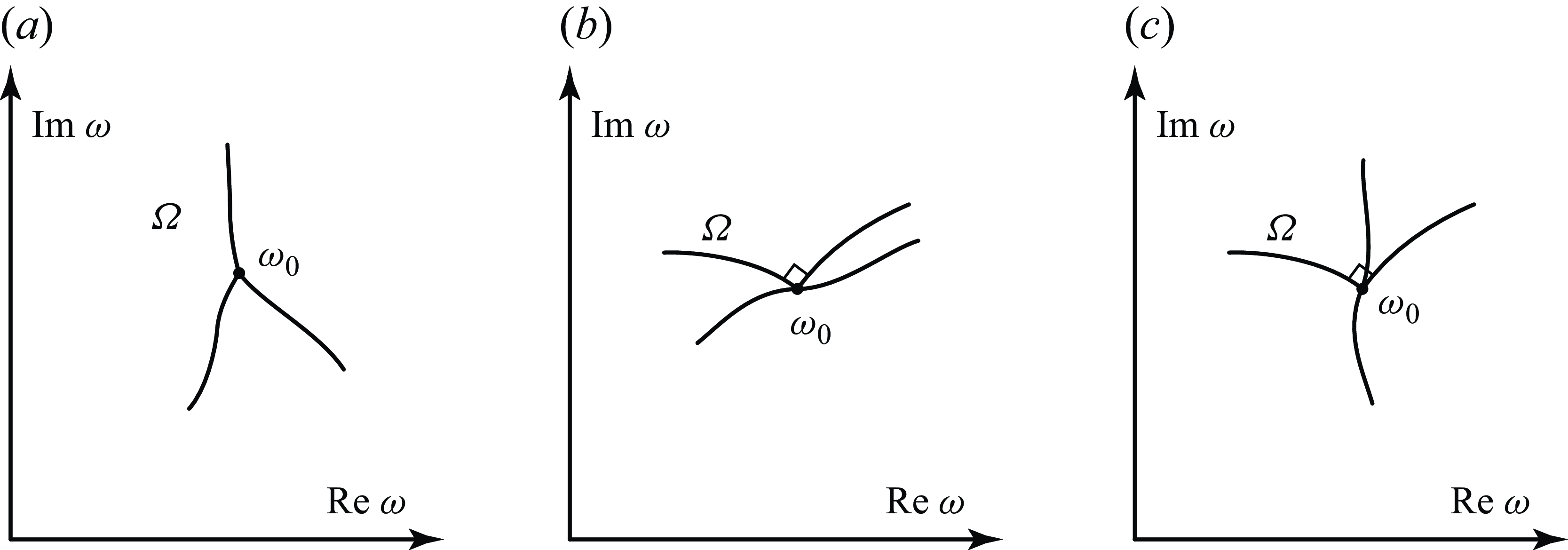
, the
$\Omega$
curve diverges in three directions; this case is shown in figure 6(a). The angles between the rays are determined by the coefficients
$a_1$
,
$b_1$
,
$c_1$
, and, generally speaking, are arbitrary.
-
(b) Case
$a_1 = b_1\not =c_1$
. In this case, the set of points on the curve is determined by the conditions(3.8)
\begin{align}\left\{ \begin{array}{l} {\textrm {Im}} ((a_2-b_2)(\omega -\omega _0)^2)=0, \quad {\textrm {Im}} ((a_1-c_1)(\omega -\omega _0))\gt 0,\\ {\textrm {Im}} ((a_1-c_1)(\omega -\omega _0)+(a_2-c_2)(\omega -\omega _0)^2)=0, \quad {\textrm {Im}} ((a_2-b_2)(\omega -\omega _0)^2)\gt 0, \\ {\textrm {Im}} ((b_1-c_1)(\omega -\omega _0)+(b_2-c_2)(\omega -\omega _0)^2)=0,\quad {\textrm {Im}} ((b_2-a_2)(\omega -\omega _0)^2)\gt 0. \end{array} \right. \end{align}
As can be seen, the last two relations give parts of the curve diverging in opposite directions, with the same tangent, but in general with different curvature. The first relation defines the parts of two perpendicularly intersecting rays lying in the half-plane
${\textrm {Im}} ((a_2-b_2)(\omega -\omega _0)^2)\gt 0$
. The resulting configurations are shown in figures 6(b,c). Since the angle between the perpendicular lines and the other straight line is arbitrary, it is possible to pass a straight section both outside (figure 6
b) and inside (figure 6
c) the angle. -
(c) Case
$a_1 = b_1 =c_1$
. The curve is determined by the expressions(3.9)Each expression specifies a part of two perpendicular lines lying in opposite sectors defined by a pair of other perpendicular curves; that is, one straight line (figure 7a ). As a result, we obtain three intersecting straight lines, the angles between which are arbitrary (figure 7 b).
\begin{align}\left\{ \begin{array}{l} {\textrm {Im}} ((a_2-b_2)(\omega -\omega _0)^2)=0, \quad {\textrm {Im}} ((a_2-c_2)(\omega -\omega _0)^2)\gt 0,\\ {\textrm {Im}} ((a_2-c_2)(\omega -\omega _0)^2)=0, \quad {\textrm {Im}} ((a_2-b_2)(\omega -\omega _0)^2)\gt 0, \\ {\textrm {Im}} ((b_2-c_2)(\omega -\omega _0)^2)=0, \quad {\textrm {Im}} ((b_2-a_2)(\omega -\omega _0)^2)\gt 0. \end{array} \right. \end{align}
Figure 6.Local structure of the
$\Omega$
curve: (a) case 3a, merging of three curves at arbitrary angles; (b,c) case 3b, four rays, two of which are perpendicular, the other two tangential.Figure 7.Local structure of the
$\Omega$
curve. (a) A set of points satisfying one of three expressions in (3.9). Sectors satisfying the inequality are shaded; solid and dashed lines satisfy the equality and fall or do not fall into the sector, respectively. (b) Case 3c, three intersecting curves.In cases (b) and (c), it was assumed that while the coefficients of the linear terms of the expansion
$k(\omega )$
coincide, the coefficients of the quadratic terms are different. The simultaneous coincidence of these and the following coefficients is not considered, because it is an extremely special case. -
-
4. Let three roots
$k_s$
,
$k_{s+1}$
,
$k_j$
at the point
$\omega _0$
have equal imaginary parts; two of them have a common branch point, and the remaining roots are different from them. Then the expansions of the roots have the form
\begin{align*} k_{s,s+1}(\omega )=k(\omega _0)\pm a\sqrt {\omega -\omega _0}+a_{1}(\omega -\omega _0)+\cdots , \end{align*}
(3.10)The equation of the curve
\begin{align} k_{j }(\omega )=k_{j}(\omega _0)+c_1(\omega -\omega _0)+\cdots. \end{align}
$\Omega$
, (3.6), is reduced to the union of the following sets:(3.11)Taking into account each equality, the corresponding inequalities can be rewritten as
\begin{align}\left\{ \begin{array}{l} {\textrm {Im}} (a\sqrt {\omega -\omega _0})=0,\quad {\textrm {Im}} (a\sqrt {\omega -\omega _0}+(a_{1}-c_1)(\omega -\omega _0))\gt 0,\\ {\textrm {Im}} (a\sqrt {\omega -\omega _0}+(a_{1}-c_1)(\omega -\omega _0))=0,\quad {\textrm {Im}} (a\sqrt {\omega -\omega _0}) \gt 0,\\ {\textrm {Im}} (-a\sqrt {\omega -\omega _0}+(a_{1}-c_1)(\omega -\omega _0))=0,\quad {\textrm {Im}} (-a\sqrt {\omega -\omega _0 })\gt 0. \end{array} \right. \end{align}
(3.12)As can be seen, the three ‘possible’ curves defined by equalities coincide in the main term, i.e. leave point
\begin{align}\left\{ \begin{array}{l} {\textrm {Im}} (a\sqrt {\omega -\omega _0})=0,\quad {\textrm {Im}} ((a_{1}-c_1)(\omega -\omega _0))\gt 0,\\ {\textrm {Im}} (a\sqrt {\omega -\omega _0}+(a_{1}-c_1)(\omega -\omega _0))=0,\quad {\textrm {Im}} ((c_1-a_{1})(\omega - \omega _0))\gt 0,\\ {\textrm {Im}} (-a\sqrt {\omega -\omega _0}+(a_{1}-c_1)(\omega -\omega _0))=0,\quad {\textrm {Im}} ((c_1-a_{1})(\omega -\omega _0))\gt 0. \end{array} \right. \end{align}
$\omega _0$
in the same direction. The inequalities determine which of these curves actually belong to
$\Omega$
, which gives us two cases.-
(a) If the first inequality is satisfied for a given direction (and, accordingly, the second and third are not satisfied), then a single curve emerges from the point
$\omega _0$
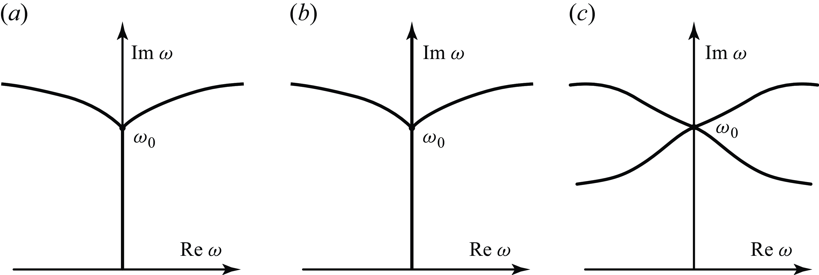
(figure 8
a). It is determined by the expression
${\textrm {Im}}\, k_s={\textrm {Im}}\, k_{s+1}\gt {\textrm {Im}}\, k_j$
. That is, the root
$k_j$
catches up with the branching pair of roots only at the branch point. -
(b) If the second and third inequalities are satisfied for a given direction (and, accordingly, the first one is not satisfied), then two curves that have a common tangent emerge from the point
$\omega _0$
(figure 8
b). They are determined by the expressions
${\textrm {Im}}\, k_s={\textrm {Im}}\, k_j\gt {\textrm {Im}}\, k_{s+1}$
and
${\textrm {Im}}\, k_{s+1}={\textrm {Im}}\, k_j\gt {\textrm {Im}}\, k_s$
, i.e. each curve is formed by the coincidence of the imaginary part
$k_j$
with one of the branching roots. In this case, there is no curve formed by two branching roots: in the latter case, the root
$k_j$
goes into the other group of roots, i.e. such a curve does not govern the asymptotic location of eigenfrequencies.
-
-
5. The last possible case of the imaginary part coincidence of the three roots
$k_s$
,
$k_{s+1}$
,
$k_j$
is their common branch point, which can be considered as a coincidence of two branch points. Then each root is represented as(3.13)Accurate to rotation and scaling of the complex plane, we can set
\begin{equation} k(\omega )=k(\omega _0)+ a(\omega -\omega _0)^{1/3}+\cdots . \end{equation}
$a=1$
. Then, denoting
$\omega -\omega _0=w\,\textrm{e}^{{i}\varphi }$
, we rewrite (3.6) as(3.14)The equalities are equivalent to
\begin{align}\left\{ \begin{array}{l} {\textrm {Im}} (\textrm{e}^{{i}\varphi /3}(\textrm{e}^{2i\unicode{x03C0} /3}-1))=0,\quad {\textrm {Im}} (\textrm{e}^{{i}\varphi /3}(\textrm{e}^{2i\unicode{x03C0} /3}-\textrm{e}^{-2i\unicode{x03C0} /3}))\gt 0,\\ {\textrm {Im}} (\textrm{e}^{{i}\varphi /3}(\textrm{e}^{-2i\unicode{x03C0} /3}-1))=0,\quad {\textrm {Im}} (\textrm{e}^{{i}\varphi /3}(\textrm{e}^{- 2i\unicode{x03C0} /3}-\textrm{e}^{2i\unicode{x03C0} /3}))\gt 0,\\ {\textrm {Im}} (\textrm{e}^{{i}\varphi /3}(\textrm{e}^{2i\unicode{x03C0} /3}-\textrm{e}^{-2i\unicode{x03C0} /3}))=0,\quad {\textrm {Im}} (\textrm{e}^{{i}\varphi /3}(\textrm{e}^{2i\unicode{x03C0} /3}-1))\gt 0. \end{array} \right. \end{align}
(3.15)Since the arguments of the numbers are respectively
\begin{align}\left\{ \begin{array}{l} \varphi /3=\unicode{x03C0} m-{\textrm {Arg}}(\textrm{e}^{2i\unicode{x03C0} /3}-1),\\ \varphi /3=\unicode{x03C0} m-{\textrm {Arg}}(\textrm{e}^{-2i\unicode{x03C0} /3}-1), \\ \varphi /3=\unicode{x03C0} m-{\textrm {Arg}}(\textrm{e}^{2i\unicode{x03C0} /3}-\textrm{e}^{-2i\unicode{x03C0} /3}). \end{array} \right. \end{align}
$5\unicode{x03C0} /6$
,
$-5\unicode{x03C0} /6$
,
$\unicode{x03C0} /2$
, satisfying the inequalities gives
$\varphi /3=\unicode{x03C0} /6$
,
$5\unicode{x03C0} /6$
,
$-\unicode{x03C0} /2$
, which yields the only direction
$\varphi =\unicode{x03C0} /2$
. This result can also be obtained from the geometric location of the cube root values when walking around the point
$\omega _0$
in the
$\omega$
plane. Thus the local behaviour of
$\Omega$
coincides with case 2: the branch point of the three roots is the end of the
$\Omega$
curve (figure 5
c).
-
6. Finally, consider the coincidence of imaginary parts of four roots
$k_s$
,
$k_{s+1}$
,
$k_j$
,
$k_{j+1}$
; we restrict ourselves by the general case when none of them have a branch point at the point of coincidence. Two types of boundary conditions in the problem are possible, which dictate two possible cases: either the
$\Omega$
curve satisfies(3.16)(symmetric configuration of coinciding roots), or
\begin{equation} {\textrm {Im}}\, k_s\gt {\textrm {Im}}\, k_{s+1}=k_j\gt {\textrm {Im}}\, k_{j+1} \end{equation}
(3.17)(non-symmetric configuration; the inequality can be reversed without loss of generality). Depending on the particular boundary conditions and expansion coefficients, from three to six rays can emerge from this point; their angles are in general arbitrary.
\begin{equation} {\textrm {Im}}\, k_s={\textrm {Im}}\, k_{s+1}\gt {\textrm {Im}}\, k_j,\ {\textrm {Im}}\, k_{j+1} \end{equation}


All possible local topologies of
 $\Omega$
of general form are considered above. Cases when the imaginary parts of five or more roots
 $k(\omega )$
coincide, and also when both the imaginary parts of the roots
 $k(\omega )$
and two or more derivatives
 ${\rm d}^pk/{\rm d}\omega ^p$
coincide, are not considered as too specific.
Local structure of the
 $\Omega$
curve: (a) case 4a, end of the
 $\Omega$
curve; (b) case 4b, merging and ending of two curves with a common tangent.

4. Bifurcations of the
$\Omega$
curve when changing the problem parameters

Assume that the physical problem under consideration has external parameters that determine the configuration of the
 $\Omega$
curve, e.g. Mach number or Reynolds number. It is obvious that with their small change, cases 1a (regular point of the curve), 2 (dead end of the curve), 3a (connection of three curves) are stable, i.e. local curve topology is not changed. The remaining cases, 1b, 1c (the intersection of two curves at angle
 $\unicode{x03C0} /2$
, or a larger number of curves at equal angles), 3b, 3c, 4a, 4b, 5, 6, in the general case, break up with an arbitrarily small change in the parameters. In this section, we analyse how such a break-up occurs.
4.1. Bifurcation of cases 1b, 1c
It is easy to see that the case 1b describes a saddle-like interaction and exchange of two segments of the curve. Indeed, the equation of the
 $\Omega$
curve in a neighbourhood of
 $\omega _0$
, accurate to rotation and scaling of the complex plane
 $\omega$
, has the form
 ${\textrm {Im}}(\varepsilon \omega +\omega ^2)=0$
. Case 1b corresponds to
 $\varepsilon =0$
; for small values of
 $\varepsilon$
, we obtain the equation of a hyperbola with asymptotes corresponding to
 $\varepsilon =0$
. This bifurcation is shown in figure 9.
The break up of the case 1c occurs in a completely similar way, with the difference that there is an interaction and exchange of three or more segments of the curve.
Bifurcation of case 1b: exchange of branches of two curves; arrows indicate the change of
 $\Omega$
curve when external parameters are changed.

4.2. Bifurcation of cases 4a, 4b
With a small change in the problem parameters, the imaginary parts of
 $k(\omega _0)$
and
 $k_j(\omega _0)$
in the expansions (3.10) become different by a small value
 $\varepsilon$
(small changes in the parameters
 $\omega _0$
,
 $a$
,
 $a_1$
,
 $c_1$
do not matter). Then the expressions (3.12) will be rewritten as
 \begin{align}\left\{ \begin{array}{l} {\textrm {Im}} (a\sqrt {\omega -\omega _0})=0,\quad {\textrm {Im}} ((a_{1}-c_1)(\omega -\omega _0))\gt \varepsilon , \\ {\textrm {Im}} (a\sqrt {\omega -\omega _0}+(a_{1}-c_1)(\omega -\omega _0))= \varepsilon , \quad {\textrm {Im}} ((c_1-a_{1})(\omega -\omega _0))\gt -\varepsilon ,\\ {\textrm {Im}} (-a\sqrt {\omega -\omega _0}+(a_{1}-c_1)(\omega -\omega _0))= \varepsilon , \quad {\textrm {Im}} ((c_1-a_{1})(\omega -\omega _0))\gt -\varepsilon . \end{array} \right. \end{align}
The first equality gives the same curve coming out of the branch point as for
 $\varepsilon =0$
. Let us consider the curves described by the second and third equalities. Without loss of generality, we set
 $a=1$
(rotation and scaling of the
 $\omega$
plane) and denote
 $z=x+iy=\pm \sqrt {\omega -\omega _0}$
,
 $a_1-c_1=\alpha +i \beta$
. Then the second and third equalities will be rewritten as
 \begin{equation} {\textrm {Im}}(z+(\alpha +i\beta )z^2)=\varepsilon\quad \Rightarrow\quad y+2\alpha xy+\beta (x^2-y^2)=\varepsilon. \end{equation}
We get the equation of the hyperbola
 \begin{gather} y=\frac {\varepsilon }{1+2\alpha x}, \quad \beta =0, \nonumber \\ \left (x+\frac {\alpha }{\beta } y\right )^2- \left (\sqrt {\frac {\alpha ^2+\beta ^2}{\beta ^2}}y-\frac {1}{2\beta }\sqrt {\frac {\beta ^2}{ \alpha ^2+\beta ^2}} \right )^2=-\frac {1}{4(\alpha ^2+\beta ^2)}+\frac {\varepsilon }{\beta },\quad \beta \not =0. \end{gather}
The part of the hyperbola satisfying the inequalities lies in the region
 $y\lt 0$
. For
 $\varepsilon =0$
, one of the branches of the hyperbola touches the straight line
 $y=0$
at the point
 $(0,0)$
; for
 $\beta \gt 0$
this branch lies at the bottom, and for
 $\beta \lt 0$
it lies in the upper half-plane
 $z$
. Depending on the sign of
 $\varepsilon$
, this branch shifts. When shifted upwards (
 $\varepsilon /\beta \gt 0$
), the curve on the plane
 $z^2=\omega -\omega _0$
has the form of a closed loop, and when shifted downwards (
 $\varepsilon /\beta \lt 0$
), it envelops the positive real semi-axis (figure 10).
Hyperbola in the
 $z$
plane (the case
 $\beta \gt 0$
is shown; for
 $\beta \lt 0$
, the picture is mirrored with respect to the real
 $z$
axis) and its mapping into the
 $\omega -\omega _0$
plane.

Now consider specifically configuration 4a, i.e. for
 $\varepsilon =0$
, the first inequality in (4.1) is satisfied, but the second and third are not satisfied (in this case,
 $\beta \gt 0$
). Then for
 $\varepsilon \gt 0$
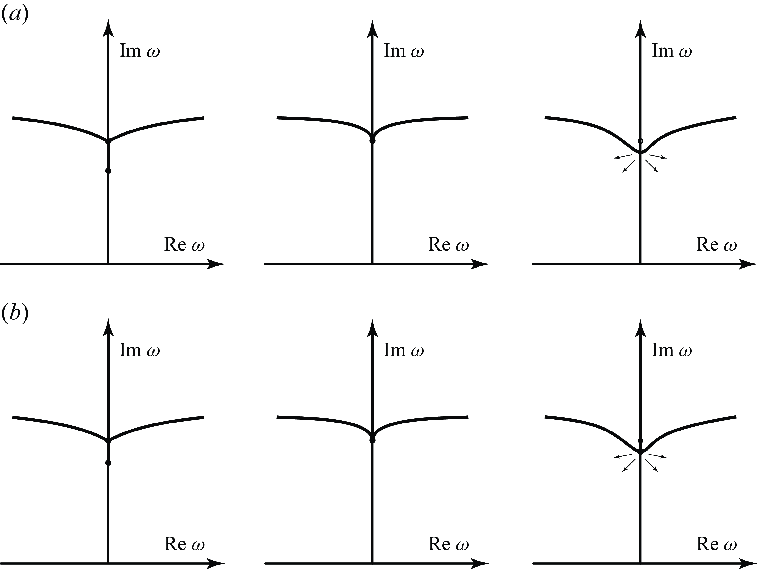
, the first inequality cuts off the part of the curve adjacent to the branch point, and instead the curve is continued by the segment described by the second and third expressions in (4.1). As a result, the curve has a loop around the branch point (the latter no longer belongs to the curve). At the point of adjoining segments of the curve, one of which is described by the first, and the other by the second and third expressions in (4.1), we have a branching of the curve, i.e. local configuration 3a. The resulting bifurcation of configuration 4a is shown in figure 11(a).
Next, consider configuration 4b, i.e. for
 $\varepsilon =0$
, the second and third inequalities in (4.1) are satisfied, but the first is not satisfied (in this case,
 $\beta \lt 0$
). Then for
 $\varepsilon \gt 0$
, the first inequality still remains unsatisfied, and the second and third inequalities describe a curve enveloping the branch point (which no longer belongs to the curve). For
 $\varepsilon \lt 0$
, the first inequality holds on the part of the curve defined by the first equality in (4.1) and adjacent to the branch point. The second and third inequalities cut off from the corresponding curve not a loop (as in case 4a), but branches going to infinity (see figure 10). As a result, we obtain the dead end of the curve, near which there is a branching of the curve. The bifurcation of configuration 4b is shown in figure 11(b).
Break up of configurations (a) 4a, (b) 4b. The original configuration is shown in the centre; the left and right plots show the curves when changing the parameters in one and the opposite direction. The dots show the dead ends of the curve (configuration 2); the circles show the branch points of
 $k(\omega )$
from the same group and, accordingly, not belonging to the curve. The arrows show the deformation of the curve when changing parameters.

4.3. Bifurcation of case 5
The common branch point of three roots
 $k_{p,q,r}(\omega )$
with a small change in parameters splits into two ‘regular’ branch points of pairs
 $k_{p,q}$
and
 $k_{p,r}$
. From the geometric analysis of the
 $k$
plane, when the parameters change in one direction, one of these points belongs to the curve, and the other does not. We get the dead end of the curve. When changing the parameters in the opposite direction, both branch points of
 $k(\omega )$
belong to the curve, and ‘sprouts’ emerge from each of them, which merge with the original part of the curve in the branching point. The resulting bifurcation is shown in figure 12.
Bifurcation of configuration 5. The original configuration is shown in the centre; on the left and right are the shapes of the curves when changing parameters in one and the opposite direction. The dots show the dead ends of the curve (configuration 2); the circle shows the branch points of
 $k(\omega )$
from the same group, which, accordingly, do not belong to the
 $\Omega$
curve. The arrows show the deformation of the curve when changing the problem parameters.

Examples of possible bifurcations of configuration 6. The original configuration is shown in the centre; on the left and right are the shapes of the curves when changing parameters in one and the opposite direction. The arrows show the deformation of the curve when changing the problem parameters.

4.4. Bifurcation of case 6
Clearly, small changes in the problem parameters make the coincidence of four
 ${\textrm {Im}}\, k$
impossible, so that this configuration breaks up into several closely located branching points (configuration 3a). There are many distinct curve topologies possible that connect those branching points. Two cases illustrating unstable merging of three and six rays are shown in figure 13. In the first case (figure 13
a), three regular branching points exist when changing parameters in one direction, and just one in the other direction. In the second case (figure 13
b), four regular branching points exist when changing parameters in any direction. Recall that the configurations shown in figure 13 are just examples; other curve topologies connecting several branching points are also possible.
4.5. Interactions of stable local topologies
From the break up of unstable topologies of the
 $\Omega$
curve analysed above, we obtain possible types of interactions of stable local topologies, because at the moment of interaction of stable topologies, an unstable one is formed. Namely, in the general case, we have the following.
-
(i) Saddle-like bifurcation of two branches of the
$\Omega$
curve shown in figure 9. -
(ii) Interaction of branching point and dead end of the curve (
$k(\omega )$
branch point belonging to the
$\Omega$
curve) is shown in figure 11(b). Intermediate unstable configuration is 4b. -
(iii) Interaction of branching and two dead ends of the curve is shown in figure 12. Intermediate configuration is fifth. The same bifurcation in the other direction of the parameter change describes the interaction of two
$k(\omega )$
branch points, in one of which branches of different groups merge (i.e. this point is a dead end of the curve), and in the other, branches from the same group merge (i.e. this point does not belong to the curve). -
(iv) Interaction of
$\Omega$
branching point and
$k(\omega )$
branch points not belonging to the curve (since
$k(\omega )$
branches from the same group merge) is shown in figure 11(a). Intermediate configuration is 4a. -
(v) Interactions of several branching points are shown in figure 13; intermediate configuration is 6. Note that after the interaction, the number of branching points can change, as shown in figure 13(a), where collapse of three branching points resulted in just one branching point remaining after the interaction.


5. Topology of the
$\Omega$
curve near the imaginary axis

5.1. Modifications of stable local tolopologies
We have considered all possible tolopogies of the
 $\Omega$
curve, except for the case when some segment of the curve includes the imaginary
 $\omega$
axis. This axis is the axis of symmetry of the complex
 $\omega$
plane. Indeed, if there is a travelling wave of the form
 $\sim \textrm{e}^{{i}(kx-\omega t)}$
, where
 $k$
and
 $\omega$
are linked by the dispersion relation, then the travelling wave
 $\sim \textrm{e}^{{i}(\hat kx-\hat \omega t)}$
(where
 $\hat k =-k^*$
and
 $\hat \omega =-\omega ^*$
are the numbers symmetric with respect to imaginary axes) describes the same wave motion, since the real parts of the exponents (which have a physical meaning) coincide. Consequently,
 $\hat k$
and
 $\hat \omega$
must also satisfy the dispersion relation, which implies the symmetry of the
 $\Omega$
curve about the imaginary axis. If part of the curve lies on the imaginary axis, then any value
 $k(\omega )$
with
 ${\rm Re}\, k\not =0$
has a paired value
 $\hat k(\omega )$
with
 ${\textrm {Im}}\, k(\omega )={\textrm {Im}}\, \hat k(\omega )$
, because in this case
 $\hat \omega =\omega$
. As a result of this pairing, all considered local configurations outside the imaginary
 $\omega$
axis have two modifications at the imaginary axis shown in figure 14: in the first, the imaginary parts of three
 $k$
coincide (one of which is purely imaginary, i.e. has no pair); in the other, the imaginary parts of two symmetric pairs
 $k$
coincide, in which
 ${\rm Re}\, k \not =0$
. The number of unstable curve topologies and options for their break up into stable ones with a small change in parameters becomes hardly countable, and their consideration in a general form does not make much sense; it is more reasonable to do this in each specific problem separately.
Coincidence of (a) three and (b) four imaginary parts of
 $k(\omega )$
roots for
 ${\rm Re}\,\omega =0$
.

Therefore, we will consider only stable local topologies and their simplest interactions.
-
(i) It is obvious that the regular point (1a), at which the imaginary parts of two
$k$
are equal, remains stable; the neighbourhood of such a regular point belongs to the imaginary
$\omega$
axis (figure 15
a). Its paired topology, in which the imaginary parts of three or four
$k$
coincide, is similar to the modification of the configuration 3a considered below. -
(ii) The local configuration 1b on the imaginary axis becomes stable: the branches of the curve emanate from the imaginary axis either at angles
$0$
,
$\unicode{x03C0}$
,
$\pm \unicode{x03C0} /2$
or at angles
$\pm \unicode{x03C0} /4$
,
$ \pm 3\unicode{x03C0} /4$
(figures 15(b,c), respectively). -
(iii) The
$k(\omega )$
branch point (configuration 2) of two
$k$
values on the purely imaginary
$k$
axis is stable and represents the dead end of the curve (figure 16
a). Its modification also exists: two symmetric branch points with
${\rm Re}\, k\not =0$
, at which pairs
$k_{p,p+1}$
and
$k_{q,q+1}$
, respectively, merge. There are two options for this modification, determined by the number of boundary conditions. To analyse this in more detail, write the expansions in the neighbourhood of the point
$\omega _0$
:(5.1)and due to the symmetry of the complex plane,
\begin{align} k_{p,p+1}(\omega )=k_p(\omega _0)\pm a\sqrt {\omega -\omega _0}+a_{1}(\omega -\omega _0)+\cdots , \nonumber \\ k_{q,q+1}(\omega )=\hat k_p(\omega _0)\pm a'\sqrt {\omega -\omega _0}+a_{1}'(\omega -\omega _0)+\cdots , \end{align}
$a'=\pm ia^*$
,
$a_1'=a_1^*$
. Let us consider possible options of the
${\textrm {Im}}\, k$
equalities: values
$k_{p,p+1}$
from a pair of branching roots, a symmetric non-branching pair
$k_p$
,
$k_q$
, and an asymmetric non-branching pair
$k_p$
,
$k_{q+1}$
. There are also (without loss of generality) two types of boundary conditions: either of the four values of
$k(\omega )$
the two largest imaginary parts coincide,
${\textrm {Im}}\, k_i={\textrm {Im}}\, k_j\gt {\textrm {Im}}\, k_{m,n}$
, or ‘intermediate’ imaginary parts coincide,
${\textrm {Im}}\, k_i\gt {\textrm {Im}}\, k_m= {\textrm {Im}}\, k_n\gt {\textrm {Im}}\, k_j$
.
Figure 15.Topology of the
$\Omega$
curve near (a) a regular point of the curve, case 1a, and (b,c) two types of case 1b.Figure 16.Shapes of the
$\Omega$
curve near the
$k(\omega )$
branch point on the imaginary axis: (a) dead end of the curve; (b) angle of the curve; (c) regular point on the curve.In the first option of the equality and the first type of the boundary conditions, we have the equation of the curve (3.6) in the form
(5.2)which is obviously impossible. With the second type of boundary conditions, we have
\begin{align} \ \ \ {\textrm {Im}}(a\sqrt {\omega - \omega_0})=0, \quad {\textrm {Im}}((a\pm a')\sqrt {\omega - \omega_0})\gt 0\ \Rightarrow\ {\textrm {Im}}(\pm a'\sqrt {\omega - \omega_0} )\gt 0, \end{align}
(5.3)In this case, we have a part of the curve
\begin{align} {\textrm {Im}}(a\sqrt {\omega - \omega_0})=0, \quad {\textrm {Im}}(a'\sqrt {\omega - \omega_0})\gt 0, \ \ {\textrm {Im}}(-a'\sqrt {\omega - \omega_0})\lt 0\ (\mathrm{or}\ {\textit{vice versa}}).\!\!\!\!\!\!\! \nonumber \\ \end{align}
$\Omega$
emanating from the paired branch point (and its symmetric reflection). Such a point is a symmetrical angle point of the
$\Omega$
curve on the imaginary axis (the curve
$\Omega$
, with the exception of the branch point, does not lie on it), as shown in figure 16(b).
Figure 17.Map of the
$\omega$
plane (a) into the
$k$
plane (b,c) in the case of a paired branch point lying on the imaginary
$\omega$
axis. Divergence of branches
$k(\omega )$
at (b) arbitrary angles, (c) horizontally and vertically.Next, let the imaginary parts of a symmetric pair of non-branching roots coincide. It follows from symmetry that this is possible only for purely imaginary
$\omega$
, and that the imaginary parts of the second pair of roots also coincide, so it is obvious that such
$\Omega$
points exist only under the first type of the boundary conditions. In this case, the curve emanates from the point
$\omega _0$
both up and down on the
$\omega$
plane, i.e. this point is not the end of the curve, but just a regular point (figure 16
c).Finally, let the imaginary parts of the asymmetric pair of non-branching roots coincide. From the symmetry of the
$k$
plane it follows that the neighbourhood of the imaginary axis
$\omega$
is mapped into different sectors of the
$k$
plane (rotated with respect to each other by a non-zero angle; see figure 17) , therefore in the general case, such equality is impossible. The exception is the case
$a=a'=\pm | a |{e}^{\pm i\unicode{x03C0} /4}$
, in which the images of the imaginary axis on the
$k$
plane diverge horizontally from the branch point (figure 17
c). In this case, the first terms of the expansion in the curve equation cancel (
$a+a'=0$
), the linear term becomes the leading one, and the equation(5.4)gives only points of the imaginary axis
\begin{equation} {\textrm {Im}} ((a_1-a_1')({\omega }-\omega _0))=0\quad \Rightarrow\quad {\textrm {Im}}(i({\omega }-\omega _0))=0 \end{equation}
$\omega$
. However, taking into account the next term of the expansion
$k(\omega )$
, of order
$(\sqrt {\omega -\omega _0})^3$
, shows that in this order, the equality of imaginary parts is generally impossible. Consideration of points close to the imaginary axis shows that this order of expansion, as well as
$\sqrt {\omega -\omega _0}$
, gives twists of the sectors of the
$k$
plane in different directions, therefore the points of
$\Omega$
ensuring the equality of the imaginary parts of an asymmetrical pair of roots do not exist.
We conclude that in addition to the dead end of the curve, with the first type of the boundary conditions, we have a continuation of the curve both up and down along the imaginary axis (at the
$k(\omega )$
branch point there is just a change in the pair of equal
${\textrm {Im}}\, k$
), as shown in figure 16(c); with the second type of the boundary conditions, we have a symmetrical angle of the curve (figure 16
b). A simple analysis shows that in the general case, both additional options are unstable, i.e. with a small change in parameters, the double branch point turns into two regular branch points. -
(iv) Let us move on to the last topology that is stable outside the imaginary axis, i.e. the branching of the curve 3a. In addition to its ‘regular’ topology, its modification exists at the imaginary axis
$\omega$
. Namely, if at the point
$\omega _0$
the imaginary parts of three
$k$
branches are equal (one of them in this case is purely imaginary), then we have the ‘regular’ branching point of the curve (figure 18
a). If the imaginary parts of two symmetric
$k$
pairs are equal (hence
${\rm Re}\, k \not =0$
necessarily), then the local topology of the curve
$\Omega$
depends on the boundary conditions. As before, write the local expansions(5.5)
\begin{align} k_s=k_s(\omega _0)+a(\omega -\omega _0),\quad k_{s+1}=k_{s+1}(\omega _0)+b(\omega -\omega _0), \end{align}
(5.6)With the first type of the boundary conditions,
\begin{align} k_p=\hat k_s(\omega _0)+a^*(\omega -\omega _0),\quad k_{p+1}=\hat k_{p+1}(\omega _0)+b^*(\omega -\omega _0). \end{align}
${\textrm {Im}}\, k_i={\textrm {Im}}\, k_j\gt {\textrm {Im}}\, k_{m,n}$
, two symmetrical branches depart from the point to the right and left, and also upward and downward branches depart along the imaginary axis
$\omega$
. That is, there is a local branching of four rays (figure 18
b). With the second type of the boundary conditions,
${\textrm {Im}}\, k_i\gt {\textrm {Im}}\, k_j={\textrm {Im}}\, k_{m}\gt {\textrm {Im}}\, k_n$
we have the intersection of two straight lines approaching the imaginary axis at an arbitrary angle; other points of the imaginary axis do not belong to the curve (figure 18
c). A simple analysis shows that both topologies are stable with respect to small changes in the problem parameters.


We conclude that not three, but seven stable local topologies of the
 $\Omega$
curve are possible on the imaginary axis: a regular point (configuration 1a), intersection of curves at angles 0,
 $\unicode{x03C0} /2$
or
 $\pm \unicode{x03C0} /4$
(two types of configuration 1b), the dead end of the curve (configuration 2), and the three types of the curve branching (configuration 3a and the two modifications). These topologies are shown in figures 15(a), 15(b), 15(c), 16(a), 18(a), 18(b), 18(c).
Configurations of the
 $\Omega$
curve near (a) the ‘regular’ branching point of the curve, and its modifications for the (b) first and (c) second types of boundary conditions.

5.2. Possible bifurcations of the curve topology in the vicinity of the imaginary axis
Since there are seven stable local configurations on the imaginary axis
 $\omega$
, six of which are non-trivial (not regular points), it is almost impossible to consider all possible interactions (the number of which is at least
 $6!=720$
) when changing the problem parameters. Therefore, in this subsection, we consider just some of the simplest interactions, which follow from consideration of break-up scenarios of unstable topologies mentioned in § 5.1.
Bifurcation of the collision of two configurations 1b.

Two options for collision of the
 $\Omega$
curve dead ends on the imaginary axis.

Namely, the following interactions are possible.
-
(i) Collision of two configurations 1b. In this case, both the first and second derivatives are equal, and structure 1c arises, after which the curve splits into three regular unconnected branches. Such a bifurcation is shown in figure 19.
-
(ii) Collision of two dead ends of the
$\Omega$
curve. Two possible bifurcations of this type are shown in figure 20. -
(iii) Collision of a dead end of the curve with a branching point of the curve. This bifurcation is topologically equivalent to the regular case (figure 11 b); after the collision, a regular section of the curve remains, as shown in figure 21(a).
-
(iv) Collision of a dead end of the curve with a modification of the branching point where four rays are connected. After the collision, a branching point of the curve remains and connects three rays, while the dead end disappears, because the
$k(\omega )$
branch point corresponds to the roots from the same group and no longer belongs to the
$\Omega$
curve. This bifurcation is shown in figure 21(b).


As mentioned above, these are just some of the possible bifurcations of the
 $\Omega$
curve topology near the imaginary
 $\omega$
axis. These bifurcations can be observed in the
 $\Omega$
curve analysis of particular problems, e.g. Podoprosvetova & Vedeneev (Reference Podoprosvetova and Vedeneev2022).
6. Examples
The results obtained above have a rather mathematical nature. However, the resulting topology of the asymptotic
 $\Omega$
curve that attracts eigenfrequencies as
 $L\to \infty$
is extremely useful in the analysis of the eigenfrequency interactions and transition to instability. Note that the equation for
 $\Omega$
does not involve boundary conditions and is governed by just the dispersion relation for the infinitely long problem. Hence the prediction on the instability and modal interactions can be made without even solving the eigenvalue problem, which can be time-consuming in many practical cases. Below, we consider several instructive problems. We start with a wave equation as a trivial example, which is followed by panel flutter in a supersonic gas flow (Dowell Reference Dowell1974; Vedeneev Reference Vedeneev2005; Shishaeva, Aksenov & Vedeneev Reference Shishaeva, Aksenov and Vedeneev2022), oscillations of a collapsible tube conveying non-Newtonian fluid (Podoprosvetova & Vedeneev Reference Podoprosvetova and Vedeneev2022), and the stability of rotating flow in a pipe (Wang & Rusak Reference Wang and Rusak1996). In all cases, we numerically trace how the elongation of the system yields the movement and interaction of eigenfrequencies in the complex
 $\omega$
plane, and their concentration near the asymptotic curves.
Collision of a dead end with a branching point connecting (a) three or (b) four rays.

6.1. Wave equation
The simplest example to demonstrate how the spectrum of the finite-length problem transforms into its limit ‘global’ state as
 $L\to \infty$
is the wave equation that is a model of a stretched string:
 \begin{equation} \frac {\partial ^2 w}{\partial t^2}-a^2\frac {\partial ^2 w}{\partial x^2}=0, \end{equation}
where
 $a$
is the speed of sound. Assuming standard boundary conditions
 \begin{equation} w(x,t)=0, \quad x=\pm \frac {L}{2}, \end{equation}
the discrete set of eigenvalues is readily given by
 \begin{equation} \omega _n=\frac {a\unicode{x03C0} n }{L}, \quad n\in \mathbb {Z}. \end{equation}
All these are real and fill the real
 $\omega$
axis as
 $L\to \infty$
. Corresponding eigenmodes have the form
 \begin{equation} w_n(x,t)=\cos \left (\frac {\unicode{x03C0} n x}{L} \right )\textrm{e}^{{-i}\omega _n t},\ n \mathrm {\ odd},\quad w_n(x,t)=\sin \left (\frac {\unicode{x03C0} n x}{L} \right )\textrm{e}^{{-i}\omega _n t},\ n \mathrm {\ even}. \end{equation}
Let us now consider the global instability approach. Considering travelling wave solutions
 $w=\textrm{e}^{{i}(kx-\omega t)}$
, we derive the dispersion relation
 \begin{equation} \omega ^2-a^2 k^2=0. \end{equation}
Solving this equation,
 $k_{1,2}(\omega )=\pm \omega /a$
, and satisfying the
 $\Omega$
curve (2.11), we conclude that the curve coincides with the real
 $\omega$
axis.
Consequently, the eigenspectrum (6.3) of the finite-length problem is just a discretisation of the
 $\Omega$
curve. Now consider the frequency selection mechanism. Eigenmodes (6.4) can be exactly represented as a superposition of two travelling waves:
 \begin{align*} w_n(x,t)=\frac {1}{2}\textrm{e}^{{i}(k_1(\omega _n)x-\omega _n t)}+\frac {1}{2}\textrm{e}^{{i}(k_2(\omega _n)x-\omega _n t)},\quad n \mathrm {\ odd}, \end{align*}
 \begin{align} w_n(x,t)=\frac {1}{2i}\textrm{e}^{{i}(k_1(\omega _n)x-\omega _n t)}-\frac {1}{2i}\textrm{e}^{{i}(k_2(\omega _n)x-\omega _n t)},\quad n \mathrm {\ even}. \end{align}
Since for each real frequency there exist just two waves travelling in opposite directions, which have no spatial growth, the reflection process described in § 2.5 does not change the wave amplitude. This ensures the perfect position of eigenfrequencies on the
 $\Omega$
curve. The selection of
 $\omega _n$
along the curve provides such a phase tuning between the two waves that after double reflection from the boundaries, the wave phase is also unchanged. Hence in the context of global instability theory, the standing wave modes (6.4) can be represented as superpositions of two travelling waves that reflect from the boundaries and transform into each other.
6.2. Panel flutter
Let us now consider a classical panel flutter problem (Dowell Reference Dowell1974): a two-dimensional elastic plate, which represents a skin panel of a supersonic aircraft, is mounted into an absolutely rigid plane and exposed to a supersonic air flow (figure 22). The problem is considered in dimensionless form, where plate thickness, plate material density and free-stream speed of sound are chosen as independent scales. Then the equation of the plate motion takes the form
 \begin{equation} \frac {\partial ^2 w}{\partial t^2}=-D \frac {\partial ^4 w}{\partial x^4}- p(x,t), \end{equation}
where
 $w$
is the vertical plate deflection,
 $D$
is the bending stiffness, and
 $p(x,t)$
is the air pressure perturbation.
Panel flutter problem: elastic plate (grey) in a supersonic gas flow.

Calculating the unsteady pressure through the piston theory,
 \begin{equation} p(x,t)=\mu \frac {M}{\sqrt {M^2-1}}\left (M\frac {\partial w}{\partial x}+\frac {\partial w}{\partial t}\right ), \end{equation}
where
 $\mu$
is the air-to-material density ratio, and
 $M$
is Mach number, we obtain the closed equation of motion:
 \begin{equation} D \frac {\partial ^4 w}{\partial x^4}+\frac {\partial ^2 w}{\partial t^2}+\mu \frac {M}{\sqrt {M^2-1}}\left (M\frac {\partial w}{\partial x}+\frac {\partial w}{\partial t}\right )=0. \end{equation}
Considering travelling wave solutions of an infinite problem,
 $w=\textrm{e}^{{i}(kx-\omega t)}$
, we obtain the dispersion relation (Vedeneev Reference Vedeneev2005)
 \begin{equation} \mathcal {D}(k,\omega )=D k^4-\omega ^2+i\mu \frac {M}{\sqrt {M^2-1}}(Mk-\omega )=0. \end{equation}
For the finite-length problem, we consider panels simply supported at both edges
 $x=\pm L/2$
(where
 $L$
is the panel length related to its thickness), i.e.
 \begin{equation} w=\frac {\partial ^2 w}{\partial x^2}=0,\quad x=\pm \frac {L}{2}. \end{equation}
For the numerical solution of the eigenvalue problem (6.9), (6.11), we use the method described by Shitov & Vedeneev (Reference Shitov and Vedeneev2016), which is not discussed here for the sake of brevity. In what follows, dimensionless stiffness and flow density are set to
 $D=23.9$
and
 $\mu =0.00012$
, which correspond to an aluminium panel at 11 km above sea level.
Spectrum of the panel flutter problem (circles) at the panel length-to-thickness ratios (a)
 $L=300$
(the panel is stable), (b)
 $L=600$
(one fluttering mode), (c)
 $L=1200$
and (d)
 $L=1600$
(multiple fluttering modes). The asymptotic
 $\Omega$
curve as
 $L\to \infty$
is shown by a grey line.

Figure 23 and supplementary movie 1 (available at https://doi.org/10.1017/jfm.2025.203) show the numerically calculated eigenspectrum of a panel in a supersonic flow with Mach number
 $M=1.5$
for different dimensionless lengths
 $L$
. When the panel length
 $L$
is small, all eigenfrequencies are damped; the increase in
 $L$
results in a decrease of their real parts, i.e. of oscillation frequencies. At certain
 $L$
, two smallest frequencies collide, and after collision, one moves down, and the other moves up into the upper half-plane, resulting in coupled-mode panel flutter. For larger
 $L$
, the following pairs of eigenfrequencies collide. The asymptotic
 $\Omega$
curve consists of three segments: one is located in the bottom half-plane and is infinite to the right; it is connected with two close-to-vertical segments at the branching point
 $\omega \approx 0.0014-0.00008i$
; each of the latter segments ends at dead ends that are
 $k(\omega )$
branch point (figure 23). It is seen that the elongation of the panel results in attraction of the numerically calculated eigenfrequencies to the
 $\Omega$
curve. Hence one can indeed predict the location of eigenfrequencies for large
 $L$
by studying the shape of the
 $\Omega$
curve without solving the eigenvalue problem. Note that the coalescence of eigenfrequencies that yields the coupled-mode flutter occurs near the branching point of the asymptotic
 $\Omega$
curve.
Instability problem of a tube conveying fluid.

The asymptotic
 $\Omega$
curve for the panel flutter case is quite simple: it has just one branching point and two dead ends of the curve (one of which, lying in the upper
 $\omega$
half-plane, is responsible for the instability). The next case represents a much more sophisticated topology of the
 $\Omega$
curve.
6.3. Instability of a tube conveying non-Newtonian fluid
As the next example, we consider axisymmetric perturbations of a finite-length elastic tube attached to two rigid tubes and conveying power-law fluid (figure 24). Taking the fluid density, steady tube radius and steady flow rate as independent scales, the non-dimensional linearised system of equations for axisymmetric perturbations under assumptions of Podoprosvetova & Vedeneev (Reference Podoprosvetova and Vedeneev2022) has the form
 \begin{align*} &\frac {\partial Q}{\partial z} + 2\unicode{x03C0} \frac {\partial R}{\partial t}=0, \end{align*}
 \begin{align*} &\frac {\partial Q}{\partial t} + \frac {2(3n+1)}{(2n+1)\unicode{x03C0} }\frac {\partial Q}{\partial z}+\frac {16n}{\unicode{x03C0}\, {Re} }Q(z,t)+\frac { 16(1-3n)}{\unicode{x03C0}\, {Re} } R(z,t)-\frac {2(3n+1)}{ (2n+1)\unicode{x03C0} }\frac {\partial R(z,t)}{\partial z} \nonumber \\& \qquad +\unicode{x03C0} \frac {\partial P}{\partial z} =0, \end{align*}
 \begin{align} P= \beta\, {R(z,t)}+m \frac {\partial ^2 R(z,t)}{\partial t^2} -N\frac {\partial ^2 R(z,t)}{\partial z^2}, \end{align}
where
 $Q(z,t)$
and
 $P(z,t)$
are the flow rate and pressure perturbations in a given cross-section, and
 $R(z,t)$
is the tube radius perturbation; parameters
 $N$
,
 $m$
,
 $\beta$
are dimensionless axial tension, linear mass density and radial stiffness of the tube;
 ${Re}$
and
 $n$
are the Reynolds number of the flow and the power-law index of the fluid rheological law. For travelling waves in an infinite-length tube, this system yields the following dispersion relation ((5.1) of Podoprosvetova & Vedeneev Reference Podoprosvetova and Vedeneev2022):
 \begin{align} \mathcal {D}(k,\omega )={}& -\frac {Nk^4}2+ \left (\frac {m \omega ^2}2+\frac {3n+1}{\unicode{x03C0} ^2(2n+1)}-\frac { \beta }2\right )k^2 \nonumber \\ {}&+\left (\frac {8 (1-3n) }{\unicode{x03C0} ^2\, {{Re}}}i -\frac {2(3n+1)}{\unicode{x03C0} (2n+1)}\omega \right )k+ \omega ^2+\frac {16n }{\unicode{x03C0}\, {{Re}}}i\omega =0. \end{align}
Axisymmetric perturbations in an infinite-length tube become unstable for the power-law index
 $n\lt 0.611$
and sufficiently small stiffness
 $\beta$
.
For the finite-length problem, neglecting rigid tube segments, and specifying fixed tube radius and pressure at both upstream and downstream ends of the elastic segment
 $z=\pm L/2$
, we obtain the following boundary conditions for perturbations:
 \begin{equation} \frac {\partial Q(-L/2)}{\partial z}=\frac {\partial Q(L/2)}{\partial z}=0,\quad P(-L/2)=P(L/2)=0. \end{equation}
The numerically calculated spectrum of the tube conveying fluid, i.e. of the system (6.12), (6.14), is shown in figure 25 and supplementary movie 2 for the parameters
 $\beta =0.1$
,
 $N=1.5$
,
 $m=0$
,
 $n=0.5$
,
 ${{Re}}=100$
, and several tube lengths. It is seen that the elongation of the tube yields more dense distribution of the eigenfrequencies and their attraction to the
 $\Omega$
curve. Sufficiently short tubes are stable; all the eigenmodes are damped and have large oscillation frequencies. Increase in
 $L$
yields the decrease of the lowest frequency down to zero, collision with its paired frequency (which is symmetrical with respect to the imaginary
 $\omega$
axis) at
 $L\approx 9.7$
, and transition to instability at
 $L\approx 9.9$
. For larger
 $L$
, next pairs of frequencies collide at the imaginary axis, and the eigenfrequencies follow a certain pattern consisting of four collisions, shown in figure 26. After passing each pattern, a couple of eigenfrequencies are moved from the bottom attractor region, which is unbounded to the left and to the right, to the upper attractor region. Namely, in figure 26, comparison of eigenfrequencies for
 $L=54.4$
and 75.0 shows that the qualitative eigenfrequency loci are similar, but for
 $L=75.0$
there are three pairs of frequencies in the upper segment, while for
 $L=54.4$
there are two pairs. Increase in
 $L$
results in saturation of the upper attractor region through similar patterns of the frequency collisions. The subsequent increase of the tube length yields the formation of a clear asymptotic structure of the eigenfrequency loci, as shown in figure 25. This structure has a quite sophisticated topology that includes two closed loops and three branching points at the imaginary
 $\omega$
axis, as well as two unbounded segments. It is clearly seen that the eigenfrequency loci tend to the
 $\Omega$
curve, although without knowing the curve topology, such distribution of eigenfrequencies would seem paradoxical. As the
 $\Omega$
curve lies entirely in the bottom
 $\omega$
half-plane, very long tubes again become stable.
Spectra of the tube conveying power-law fluid (circles) for
 $L=50$
, 100, 200, 500. The asymptotic
 $\Omega$
curve as
 $L\to \infty$
is shown by a grey line.

From this example, we conclude that the analysis of the
 $\Omega$
curve topology yields a deep understanding of the eigenfrequency distribution in the
 $\omega$
plane, even though it is very unusual at first sight. As in the panel flutter example, we also observe eigenfrequency coalescence near branching points of the
 $\Omega$
curve. This feature helps to explain the nature of the frequency coalescence, which can yield the coupled-mode instability in various systems involving fluid–structure interactions.
Pattern of the eigenfrequency collisions with the increase of
 $L$
that results in transferring of a pair of frequencies from the bottom attractor region to the upper attractor region. Arrows show the frequency loci for increasing
 $L$
.

Rotating fluid flow in a pipe.

6.4. Instability of rotating pipe flow
As a last example, let us analyse the flow of inviscid fluid in a pipe, following the study of Wang & Rusak (Reference Wang and Rusak1996). The fluid performs columnar axial motion and simultaneous solid body rotation (figure 27). Considering the dimensionless problem with the axial velocity and radius taken as independent scales, the base velocity in the cylindrical coordinate system
 $(r,\theta , z)$
takes the form
 \begin{equation} u_r=0, \quad u_{\theta }=\frac {\sqrt {\Omega }}{2}r, \quad u_z=1, \end{equation}
where
 $\sqrt {\Omega }$
is a swirl parameter. The equation of motion for small perturbations has the form (Wang & Rusak Reference Wang and Rusak1996)
 \begin{equation} \left (\psi _{yy}+\frac {\psi _{zz}}{2y}+\frac {\psi }{2y}\right )_{zz}+ 2\left (\psi _{yy}+\frac {\psi _{zz}}{2y}\right )_{zt}+ \left (\psi _{yy}+\frac {\psi _{zz}}{2y}\right )_{tt}=0, \end{equation}
where
 $\psi (z,y,t)$
is a stream function perturbation,
 $y=r^2/2$
, and subscripts denote differentiation. Considering axisymmetric perturbations, the function
 $\psi$
must satisfy kinematic boundary conditions at the pipe axis and the wall,
 $\psi (z,0,t)=\psi (z,1/2,t)=0$
. Separation of variables
 $\psi (z,y,t)=\varphi (z)\,\Phi (y)\,\textrm{e}^{{-i}\omega t}$
yields the equation for
 $\varphi (z)$
:
 \begin{equation} \varphi ''''-2i\omega \varphi '''+(\Omega -\Omega _B-\omega ^2)\varphi ''+2i\omega \Omega _B\varphi '-\omega ^2\Omega _B\varphi =0, \end{equation}
where a prime stands for the
 $z$
-derivative, and
 $\Omega _B=14.682$
is a critical swirl parameter.
The corresponding dispersion relation in the notation of the present paper is
 \begin{equation} (k^2+\Omega _B)(k-\omega )^2-\Omega k^2=0. \end{equation}
Note that wavenumber and frequency parameters used by Wang & Rusak (Reference Wang and Rusak1996) are related to the present paper’s parameters as
 $\sigma =-i\omega$
and
 $\alpha =ik$
.
A simple analysis of the dispersion relation (6.18) shows that as
 ${\textrm {Im}}\,\omega \to +\infty$
, three roots
 $k(\omega )$
have positive, and one negative, imaginary parts. Consequently, the flow admits three right-travelling waves and one left-travelling wave. According to § 2.1, for the finite-length flow, we must set three boundary conditions at the inlet pipe cross-section, and one condition at the outlet cross-section. A particular form of these conditions was suggested by Wang & Rusak (Reference Wang and Rusak1996):
 \begin{equation} \varphi =\varphi ''=(\Omega _B-\Omega )\varphi '-\varphi '''=0, \ z=-\frac {L}{2}, \quad \varphi '=0, \ z=\frac {L}{2}. \end{equation}
The calculated spectrum of the boundary value problem (6.17), (6.19) is shown in figure 28 and supplementary movie 3 for the swirl parameter
 $\Omega =15.182\gt \Omega _B$
. For very short pipes,
 $L\lt 2.2$
, there is just one damped eigenmode lying on the imaginary
 $\omega$
axis. Increase in
 $L$
yields its motion up along the imaginary axis, and at
 $L\approx 2.2$
, it moves into the upper half-plane; the flow becomes unstable (figure 28
a). This mode was previously analysed by Wang & Rusak (Reference Wang and Rusak1996); the instability takes place for
 $\Omega \gt \Omega _1=\Omega _B+\unicode{x03C0} ^2/4L^2$
.
More interesting phenomena occur when the pipe length is increased further. In contrast to previously considered problems, where the spectrum is countable, the rotating flow problem has a finite number of eigenmodes for any
 $L$
. However, the number of modes increases when the length
 $L$
is increased: at certain values of
 $L$
, new modes appear from infinity at the negative imaginary ray and move up along the imaginary axis. Such unusual behaviour is due to specific properties of the dispersion relation (6.18) at large
 $|\omega |$
: the function
 ${\textrm {Im}}\, k_3(\omega )-{\textrm {Im}}\, k_4(\omega )\sim c_2+c_2/\omega ^2$
as
 $\omega \to \infty$
so that the expansion (2.12) is losing power at large
 $|\omega |$
. The second mode penetrates into the upper
 $\omega$
half-plane at
 $L\approx 6.7$
, and almost immediately collides with the first mode, yielding two oscillatory unstable modes (figure 28
b). The next pair of non-oscillatory eigenfrequencies penetrates into the upper half-plane at
 $L\approx 11.1$
(figure 28
c) and
 $L\approx 15.5$
; they collide and become oscillatory at
 $L\approx 15.6$
. Further increase in
 $L$
yields the appearance of more and more eigenfrequencies that follow the same pattern. As can be seen in figure 28(d), their limit locations tend to the
 $\Omega$
curve, which has three segments: one is infinitely long and occupies the negative imaginary ray, and two more segments are finite and connect the branching point
 $\omega =0$
with dead ends
 \begin{equation} \omega =\pm \sqrt {\Omega _B}\left (\left (\frac {\Omega }{\Omega _B}\right )^{1/3}- 1\right )^{3/2} \approx \pm 0.00456. \end{equation}
Spectrum of the rotating pipe flow for (a)
 $L=5$
(one non-oscillatory instability mode of Wang & Rusak Reference Wang and Rusak1996), (b)
 $L=8$
(two oscillatory instability modes), (c)
 $L=13$
(three instability modes), and (d)
 $L=40$
(nine instability modes). The asymptotic
 $\Omega$
curve as
 $L\to \infty$
is shown by a grey line.

The configuration of the
 $\Omega$
curve explains the seeming contradiction: the infinite problem is neutrally stable, while the finite-length problem is unstable for arbitrarily large
 $L$
(Wang & Rusak Reference Wang and Rusak1996). At first sight, this breaks the principal global instability property (§ 2.4): if the finite-length system is globally unstable, then the infinite-length system is also unstable. However, in the rotating flow problem, the system is neutrally globally stable: the
 $\Omega$
curve has a segment of real frequencies, but does not have points with
 ${\textrm {Im}}\,\omega \gt 0$
. The instability that takes place is a purely finite-length phenomenon attributed to the specific boundary conditions. As dictated by the
 $\Omega$
curve, the growth rates have
 ${\textrm {Im}}\,\omega _n\to 0$
as
 $L\to \infty$
, but the global instability theory a priori provides no information on the side of the curve to which the eigenfrequencies are attracted, i.e. on the sign of
 ${\textrm {Im}}\,\omega _n$
. For the set of boundary conditions (6.19),
 ${\textrm {Im}}\,\omega _n\to +0$
, but it is generally possible that another set of conditions yields
 ${\textrm {Im}}\,\omega _n\to -0$
, thus ensuring the finite-length flow stability. It is, of course, important which boundary conditions represent the real physical flow, and we believe that those suggested by Wang & Rusak (Reference Wang and Rusak1996) are reasonable so that such flow is actually unstable for any
 $L$
.
7. Conclusions
We have studied possible configurations of the asymptotic curve
 $\Omega$
that attracts eigenfrequencies of a long but finite system as length
 $L\to \infty$
. The set of stable configurations consists of a regular point, a dead end of the curve, and a connection of three curves. Note that at the dead end of the curve,
 $k(\omega )$
has a branch point, and the reverse function
 $\omega (k)$
has a saddle point, which is associated with absolute instability of an infinitely long system. Bifurcations of the curve topology when changing the problem parameters are analysed. The case of the imaginary axis is special: is has seven stable configurations of the curve, and a huge number of possible topology bifurcations.
The examples of the
 $\Omega$
curve topology provided in this study deal with supersonic panel flutter (Vedeneev Reference Vedeneev2005, Reference Vedeneev2016; Vedeneev et al. Reference Vedeneev, Guvernyuk, Zubkov and Kolotnikov2010), a pipe conveying non-Newtonian fluid (Podoprosvetova & Vedeneev Reference Podoprosvetova and Vedeneev2022), and rotating pipe flow (Wang & Rusak Reference Wang and Rusak1996), where several bifurcations of the topology are observed when changing the problem parameters. However, the applications of the asymptotic analysis are not limited to these problems; the global instability analysis has been used successfully in a wide variety of processes, such as Poiseuille flow in a pipe of finite length, thermocapillary convection, jet flows, elastic plates in an incompressible fluid flow, spiral waves, flame stability, Couette flow of magnetic fluid, bending vibrations of pipes conveying fluid, flow over cavities, and plasma instability; see Doaré & de Langre (Reference Doaré and de Langre2006)and Vedeneev (Reference Vedeneev2016) for details.
The principal limitation of the global instability analysis is that it is valid for sufficiently long domains, but the actual range of suitable lengths is a priori not known. In the panel flutter problem, real skin panels of supersonic aircrafts perfectly follow the predictions of the global instability theory at their real lengths (
 $\sim 300$
thicknesses). However, the fluid-conveying elastic tube closely follows the
 $\Omega$
curve only at really large length (
 $\sim 500$
radii); in this globally stable case, the finite-length tube stays unstable up to lengths
 $\sim 200$
radii, and stabilises only at larger lengths. The rotating pipe flow demonstrates probably the most unexpected case: the flow is globally neutrally stable, but calculated growth rates tend to zero as
 $L\to \infty$
staying positive, i.e. the flow stays unstable for arbitrarily large
 $L$
. This is an exceptional case of neutral global stability, when the actual stability or instability of a finite-length problem depends on particular boundary conditions and cannot be predicted without consideration of the full eigenvalue problem.
The advantage of the global instability analysis is that the
 $\Omega$
curve for a particular physical system can be obtained in a closed form without solving the eigenvalue problem. Moreover, even if the physically reasonable lengths of the system are not large enough to closely follow the global instability theory predictions, the pattern of the eigenfrequency loci in the complex plane is very well predicted by the
 $\Omega$
curve even for very short lengths, as demonstrated by all examples considered in this paper. This feature can be used for the control of instability by preventing the formation of unstable modes in advance. Given that the analysis of the
 $\Omega$
curve yields the effective understanding of eigenfrequency interactions and the nature of possible instabilities, it is an effective and powerful tool for the analysis of a variety of physical problems.
Supplementary movies.
Supplementary movies are available at https://doi.org/10.1017/jfm.2025.203.
Acknowledgements.
We dedicate this work to the memory of Professor A.G. Kulikovskii (1933–2024), academician of the Russian Academy of Sciences. His pioneering works in magnetohydrodynamics, stability of fluid and plasma flows, and shock waves in elastic media, affected literally all fields of modern mechanics. He was also an outstanding teacher who supervised several generations of scholars in the Soviet Union and later in Russia. We were privileged to be his students, and benefited from continuous support and personal communications with this outstanding scientist.
Funding.
The contribution of V.V. was supported by the Russian Science Foundation under grant no. 19–71-30012, and performed at Steklov Mathematical Institute of the Russian Academy of Sciences.
Declaration of interests.
The authors report no conflict of interest.