1. Introduction
In engineering practice, multiple cylindrical structures that share the same fundamental form but are in different isomeric configurations are frequently encountered, for example, the bridge deck and main cable. The free shear layer separated from the leading edge of a rectangular cylinder-like bluff body (bridge deck) plays an important role in determining the aerodynamics of the circular one (main cable), and vice versa. However, previous studies have primarily focused on the aerodynamics of arrangements of bluff bodies with the same geometries (Zhou & Yiu Reference Zhou and Yiu2006; Ren et al. Reference Ren, Liu, Cheng, Tong and Xiong2023; He et al. Reference He, Wu, Peng, Zou, Jing, Yan, Guo, Dong and Li2024; Zhang et al. Reference Zhang, Tang, Lu, Jin, An and Cheng2024; Zhao et al. Reference Zhao, Wang, Zhu, Cao, Bao, Zhou, Cheng and Han2024; Zhou, Hao & Alam Reference Zhou, Hao and Alam2024). The fluid dynamics of an isomeric bluff-body system is more complex than isomorphic bluff-body systems because of their significant diverse geometries. Therefore, detailed investigations into their aerodynamics are of both scientific and practical interest.
Bluff-body systems in isomeric configurations in engineering practice typically consist of rectangular cylinders, circular cylinders and other polygonal cylinders. As for rectangular cylinder, its flow behaviour is sensitive to width-to-height ratio (B/D). Three dominant flow structures have been identified: (a) leading-edge vortex shedding (LEVS), (b) trailing-edge vortex shedding (TEVS) (Nakamura, Ohya & Tsuruta Reference Nakamura, Ohya and Tsuruta1991; Naudascher & Rockwell Reference Naudascher and Rockwell2012; Cimarelli, Corsini & Stalio Reference Cimarelli, Corsini and Stalio2024; Païdoussis et al. Reference Païdoussis, Price and De Langre2010) and (c) global instability induced by complex interactions between LEVS and TEVS (Hourigan et al. Reference Hourigan, Mills, Thompson, Sheridan, Dilin and Welsh1993; Li et al. Reference Li, Jiang, Liu, Wang and He2024a ; Mills et al. Reference Mills, Sheridan and Hourigan2002, Reference Mills, Sheridan and Hourigan2003; Tan, Thompson & Hourigan Reference Tan, Thompson and Hourigan2004). Generally, Kelvin–Helmholtz vortices are generated through LEVS and evolve into hairpin vortices; simultaneously, TEVS takes place and leads to the formation of a von Kármán-like street in the wake (Li et al. Reference Li, Wang, Qiu, Zhou, Fu and Liu2024b , Reference Li, Wang, Qiu, Zhou, Fu and Liu2024c ). In the study of global instability, Naudascher & Rockwell (Reference Naudascher and Rockwell1994) introduced the term ‘impinging leading-edge vortex (ILEV) instability’ to reflect the fact that it is primarily the large-scale vortices shed from the leading-edge separated flow that interact with the trailing edge, rather than the separated flow itself. The interactions between LEVS and TEVS have been widely investigated for 3 ≤ B/D ≤ 12. As a direct consequence of these interactions, ILEV emerges and induces two distinct self-sustained oscillation feedback mechanisms, which have likewise been thoroughly examined for 3 ≤ B/D ≤ 8 (Mills, Sheridan & Hourigan Reference Mills, Sheridan and Hourigan2003; Sarwar et al. Reference Sarwar, Ishihara, Shimada, Yamasaki and Ikeda2008; Zhang et al. Reference Zhang, Kareem, Xu and Jiang2023). For an elongated rectangular cylinder (B/D>12), the flow is characterised by a large-scale separation bubble originating from LEVS, as illustrated in figure 1(a). The leading-edge separated flow reattaches at the surface of the rectangular cylinder, with the reattachment point located approximately 5D from the windward side. Studies on the effects of the Reynolds number (Re = U ∞ ⋅ D/ν), where U is a characteristic speed and ν is the kinematic viscosity, on the flow around a rectangular cylinder indicate that it has a limited influence on mean flow statistics (Zhang et al. Reference Zhang, Kareem, Xu and Jiang2023; Cimarelli et al. Reference Cimarelli, Corsini and Stalio2024; Samsam-Khayani & Seyed-Aghazadeh Reference Samsam-Khayani and Seyed-Aghazadeh2025). In particular, the streamwise length of the primary vortex (measured as the reattachment length) only slightly increases with Re (Cimarelli et al. Reference Cimarelli, Corsini and Stalio2024). However, Re has a significant effect on the stability of the leading-edge separated flow (Zhang et al. Reference Zhang, Kareem, Xu and Jiang2023). For Re < 2000, the leading-edge separated flow steadily reattaches to the rectangular cylinder’s surface. As Re increases, the leading-edge separated flow becomes progressively more unstable, eventually leading to the development of ILEV instability at Re ≈ 300 (Okajima Reference Okajima1982; Nakamura et al. Reference Nakamura, Ohya, Ozono and Nakayama1996). By further increasing Re, regular vortex shedding is weakened. For B/D > 12 in particular, the velocity spectra are broad with no dominant peaks for Re>2000 (Mills et al. Reference Mills, Sheridan and Hourigan2002, Reference Mills, Sheridan and Hourigan2003; Nakamura et al. Reference Nakamura, Ohya and Tsuruta1991; Samsam-Khayani & Seyed-Aghazadeh Reference Samsam-Khayani and Seyed-Aghazadeh2025). Consequently, the characteristic signature of ILEV instability is likely obscured by background turbulence fluctuations and often difficult to identify at high Re and large B/D. The above discussion suggests that the dependence of the flow around a rectangular cylinder on B/D is quite complex. If a circular cylinder is placed in its leading-edge separated flow, the flow interactions between them shall be further complicated, but studies on such scenarios are quite limited. To reveal the flow mechanisms underlying this isomeric cylinder configuration, it is preferable to consider an elongated rectangular cylinder, which effectively eliminates the influence of ILEV instability as a first step, as illustrated in figure 1(a).
(a) Schematic diagram of flow around an elongated rectangular cylinder. (b) Position I: a circular cylinder beyond the reattachment point. (c) Position II: a circular cylinder near the leading-edge separation bubble.

For a circular cylinder situated beyond the reattachment point, its flow behaviours mimic to those of a near-wall circular cylinder, as shown in figure 1(b). Most research on a circular cylinder near a wall focuses on the flow properties and aerodynamic characteristics of the circular cylinder (He et al. Reference He, Pan, Feng, Gao and Wang2016, Reference He, Wang, Pan, Feng, Gao and Rinoshika2017a
; Zhou et al. Reference Zhou, Qiu, Li and Liu2021; Li et al. Reference Li, Wang, Qiu, Wu, Zhou, Fu and Liu2022; Tong et al. Reference Tong, Cheng, An, Griffiths and Ren2025) as well as the effect of the circular cylinder on the wall boundary layer (Zhou et al. Reference Zhou, Qiu, Li and Liu2022; Wang et al. Reference Wang, Zhou, Chen, Sung, Liu and Wu2024a
; Bista et al. Reference Bista, Fredrick-Smiles, Nasif and Balachandar2025). Recently, notable progress has been made in other aspects of the fluid mechanics of near-wall cylinders (Li et al. Reference Li, Wang, Qiu, Zhou, Fu and Liu2025a
, Reference Li, Wang, Qiu, Zhou, Fu and Liu2025b
), including the effects of a short splitter plate on near-wall circular cylinder flow (Zhou et al. Reference Zhou, Qiu, Li and Liu2025), wake asymmetry in channel-confined flows (Lu et al. Reference Lu, Aljubaili, Zahtila, Chan and Ooi2023), turbulent wake characteristics near moving walls (Kim, Kim & Lee Reference Kim, Kim and Lee2023; Jiang et al. Reference Jiang, Ju, Guo and Wang2024), and the effects of magnetic fields on cylinder-wall interactions (Wang et al. Reference Wang, Zhang, Kolesnikov, Lyu, Yang, Ni and Zhang2024b
). Generally, the flow properties and aerodynamic characteristics of a near-wall circular cylinder are particularly sensitive to gap-to-diameter ratio G/D, where D and G are the cylinder diameter and the gap between the cylinder and wall, respectively. When G/D < 0.5, a recirculation eddy forms within the wall boundary layer upstream of the forebody of the circular cylinder, while intensity-weakened alternate vortex shedding occurs in its near wake (Lin et al. Reference Lin, Lin, Hsieh and Dey2009; Tong et al. Reference Tong, Cheng, An, Griffiths and Ren2025). When 0.5 ≤ G/D ≤ 1.0, there are three shear layers in the region downstream of the cylinder: the free shear layers from the upper and lower surfaces of the circular cylinder and the boundary layer on the wall (Lei et al. Reference Lei, Cheng and Kavanagh1999, Reference Lei, Cheng, Armfield and Kavanagh2000). The boundary layer on the bottom wall couples with the shear flow from the lower side of the circular cylinder and deflects away from wall, which is known as shear layer pairing rather than shear layer counteracting (Price et al. Reference Price, Sumner, Smith, Leong and Paidoussis2002; Sarkar & Sarkar Reference Sarkar and Sarkar2010). With a further increase in G/D beyond 1.0, shear layer pairing significantly reduces (He et al. Reference He, Wang, Pan, Feng, Gao and Rinoshika2017a
), and the distribution of mean vorticity in the near wake becomes approximately symmetric about its horizontal central line. Moreover, a dominant frequency characterised by a Strouhal number (
 $\mathit{St}\mathit{=}\mathit{f}\mathit{\boldsymbol{\cdot }}\mathit{D}\mathit{/}\mathit{U}_{\mathit{\infty }}$
) increases as G/D decreases,
 $f$
denotes the vortex shedding frequency ; this is caused by the combined effects of the deflected gap flow and the velocity gradient (Zhou et al. Reference Zhou, Qiu, Li and Liu2022). In addition, several other coherent structures around a near-wall cylinder have been studied, including Lagrangian coherent structures (He et al. Reference He, Pan, Feng, Gao and Wang2016), a von Kármán vortex street (Zhou et al. Reference Zhou, Qiu, Li and Liu2021), hairpin-like vortices (Li et al. Reference Li, Wang, Qiu, Wu, Zhou, Fu and Liu2022) as well as Λ-shaped structures (Tong et al. Reference Tong, Cheng, An, Griffiths and Ren2025). These turbulent structures can be classified as vortex dynamics near a circular cylinder in proximity to the wall. With respect to aerodynamic characteristics, the pressure field properties of a near-wall cylinder can be categorised into two cases in the three flow regimes discussed above (Yang, An & Cheng Reference Yang, An and Cheng2018). Particularly, the pressure distribution on the circular cylinder is sensitive to Re for G/D > 0.5 but not for G/D
 $\leq$
0.5. However, compared with an isolated circular cylinder, the above-mentioned studies have fully revealed the fluid dynamics of a circular cylinder in proximity to a wall with the variation of G/D. Building on this foundation, the present work further incorporates the influence of leading-edge separated flow generated by an elongated rectangular cylinder, as illustrated in figure 1(c).
For a circular cylinder situated near the leading-edge separated flow, the two circular cylinders in isomorphic configuration provide valuable insights. The flow fields for these isomorphic cylinders involve complex interactions between the shear layers, vortices and wakes, which were of early interest (Chen Reference Chen1985; Nishimura, Ohori & Kawamura Reference Nishimura, Ohori and Kawamura1986; Ohya et al. Reference Ohya, Okajima, Hayashi and Cheremisinoff1989; Zdravkovich Reference Zdravkovich1977, Reference Zdravkovich1985). Studies have typically focused on the interaction of the flow structures between two cylinders of equal diameter with varying
 $l$
denotes the centre-to-centre distance and incidence angle α. These configurations are generally grouped into three types: (a) cylinders in tandem configuration, (b) cylinders in side-by-side configuration and (c) cylinders in staggered configuration. The corresponding fluid behaviours can be classified into two fundamental types of interferences (Zdravkovich Reference Zdravkovich1987): (i) wake interference, which occurs when one cylinder is partially or entirely immersed in the wake of the other, and (ii) proximity interference, which arises when the two cylinders are in close proximity without either being immersed in the wake of the other. On the basis of these two fluid behaviours, distinct flow regimes have been identified. For the case of two tandem circular cylinders, these are the extended-body regime (1 < l/D < 2), reattachment regime (2 < l/D < 5) and co-shedding regime (l/D > 5) (Zhou & Yiu Reference Zhou and Yiu2006), whereas the flow patterns of two side-by-side circular cylinders can been classified into isolated bluff-body behaviour (1 < l/D < 1.2), a biased flow pattern (1.2 < l/D < 2.2) and parallel vortex streets (l/D > 2.2) (Sumner Reference Sumner2010). The flow patterns around two staggered circular cylinders can be classified according to α into cases with an isolated bluff body, a small incidence angle and a large incidence angle (Sumner, Price & Paidoussis Reference Sumner, Price and Paidoussis2000). The aerodynamic characteristics, including static pressure distributions, vortex shedding frequencies and lift and drag forces, have been analysed to corroborate these flow features. For instance, two distinct von Kármán vortex shedding processes have been detected for staggered-cylinder configurations depending on the vortex shedding frequency (Kiya et al. Reference Kiya, Arie, Tamura and Mori1980), and pressure coefficient data have been obtained as evidence to witness the fluid behaviours mentioned above, revealing a stable pair of eddies in the gap between two tandem cylinders, and continuous reattachments of the two shear layers (Hiwada, Mabuchi & Yanagihara Reference Hiwada, Mabuchi and Yanagihara1982; Igarashi Reference Igarashi1981, Reference Igarashi1984; Ljungkrona Reference Ljungkrona1992). Recently, advancements in computer technology and numerical models have enabled a deeper understanding of the flow characteristics of two cylinders in cases of high Reynolds numbers. It has been observed that a higher Re results in a thinner boundary layer and an upstream shift of the cylinders’ flow separation point, as well as a sudden change in the near-wake vortex street. This sudden change manifests as spontaneous intermittent transitions between distinct flow regimes (e.g. from an isolated bluff-body mode to biased gap flow) driven by high-Reynolds-number instabilities, which subsequently affect the Strouhal number of the cylinders (Xu, Zhou & So Reference Xu, Zhou and So2003; Zhou et al. Reference Zhou, Feng, Alam and Bai2009; Wu et al. Reference Wu, Du and Wang2020a
,Reference Wu, Lin, Du, Shi and Zhu2020b
). This classification of flow regimes for two circular cylinders provides a useful foundation for the present research. However, the free shear layer of two circular cylinders differs significantly from the separation bubble generated by an elongated rectangular cylinder. Therefore, further investigation is warranted.
Guided by the previously discussed work from the existing literature, this study considers an elongated rectangular cylinder with B/D = 14 to examine the effect of the rectangular cylinder leading-edge separated flow on the aerodynamics of a circular cylinder in a regime that minimises the effects of the TEVS generated by the rectangular cylinder. Section 2 provides details of the wind tunnel configurations, test models and experimental set-ups. In § 3, the flow around the circular–rectangular system is qualitatively and quantitatively visualised using smoke-wire and particle image velocimetry (PIV) methods, respectively; then, lift power spectral densities and pressure distributions are introduced, and three typical flow patterns around the circular cylinder near the leading edge of an elongated rectangular cylinder are identified. In § 4, the aerodynamic forces of circular cylinder in the above-mentioned three flow regimes are discussed. Finally, § 5 summarises the main conclusions of the study.
Experimental set-ups: (a) wind tunnel test section and model installations, (b) flow profiles of the test section, (c) test cases and (d) pressure tap configuration (unit: mm).

2. Experimental details
2.1. Wind tunnel and experimental model
All the experiments were conducted in a closed-loop wind tunnel (CSU-WT2) with a test section of 1500 mm (length)
 $\times$
800 mm (width)
 $\times$
1200 mm (height), as shown in figure 2(a). The incoming flow velocity U
∞
could be modulated continuously from 0.5 to 30 ms−1; the corresponding flow profiles in the wind tunnel test section at U
∞
= 2 ms−1 without any other turbulence generators are shown in figure 2(b). Generally, the thickness of the boundary layer was δ ≈ 100 mm and the turbulence intensity out of the boundary layer was lower than 0.5 %. In the present study, a pitot tube was fixed at 150 mm from the ceiling of the wind tunnel to monitor the total and static pressures of the incoming flow. For clarity of presentation, a Cartesian coordinate system was established at the entrance of the test section: the x-, y- and z-axes represent the streamwise, spanwise and transverse flow directions, respectively.
The test model consisted of a circular cylinder made from highly transparent organic glass which allowed a laser to illuminate the entire flow field surrounding the circular cylinder. The diameter and spanwise length of the circular cylinder were D = 60 mm and L = 800 mm, respectively, resulting in a blockage ratio of 5 %. The influences of wind-induced micro-vibration and wall-induced laser reflection on the experimental results were minimised by using an elongated rectangular cylinder made of carbon fibre with a surface coated with black matte paint. All the tested cases are illustrated in figure 2(c). The tested gap-to-diameter ratios, G/D, were 0, 0.1, 0.2, 0.3 and 0.4, and the distance-to-diameter ratios, L/D, were 0.6, 1.6, 2.02, 3.0, 3.56, 4.4 and 5.8.
2.2. Pressure and aerodynamic forces
As shown in figure 2(d), 38 pressure taps with an inner diameter of 0.8 mm were pre-installed on the middle span of the circular cylinder, with an angular interval of 8° for taps 8–13 and 27∼32 and 10° for taps 1–8, 13–27 and 32–38. Each pressure tap was connected to one channel of a ZOC33/64PxX2 scanner via the same tubing system as used in Li et al. (Reference Li, He, Wang and Kareem2019) but with a length of 500 mm. The signals from the pitot tube were also recorded by this pressure scanner system. A total of 20 000 samples were recorded at a sampling frequency of 325 Hz for each pressure channel. The dominant frequency of the pressure fluctuations observed on the present circular cylinder model was approximately 30 Hz. In prior work (Li et al. Reference Li, He, Wang and Kareem2019), an uncertainty of 5.13 % was recorded for the pressure field measurement. This distortion was avoided in this study by employing the correction method proposed by Bell et al. (Reference Bell, Burton, Thompson, Herbst and Sheridan2016).
The pressure coefficients around the tested model were obtained as follows:
 \begin{align} \overline{C_{\!P}}&=\left(\overline{P}-P_{s}\right)/\left(0.5\rho U_{\infty }^{2}\right)\! , \end{align}
 \begin{align} C^{\prime}_{\!P}&=\sqrt{\sum \left(P-\overline{P}\right)^{2}/n}/\left(0.5\rho U_{\infty }^{2}\right)\! , \end{align}
where
 $\mathit{P}$
is the measured pressure at each pressure tap,
 $\overline{\mathit{P}}$
is the time-averaged pressure,
 $\mathit{P}_{\mathrm{s}}$
is the static pressure in the test section of the wind tunnel,
 $\mathit{P}_{{dyn}}\mathit{=}0.5\mathit{\rho }\mathit{U}_{\mathrm{\infty }}^{2}$
is the dynamic pressure of the incoming flow and
 $\rho$
denotes the air density. Both
 $\mathit{P}_{\mathrm{s}}$
and
 $\mathit{P}_{{dyn}}$
were measured using pitot tubes.
Aerodynamic force coefficients were calculated by integrating the measured pressure over the cylinder’s surface. Statistical analysis was performed to obtain the time-averaged drag coefficient
 $\mathit{C}_{\!\mathit{D}}$
, the fluctuating drag coefficient
 $\mathit{C}_{\!\mathit{D}}^{\prime}$
, the time-averaged lift coefficient
 $\mathit{C}_{\mathit{L}}$
and the fluctuating lift coefficient
 $\mathit{C}_{\mathit{L}}^{\prime}$
. Since the experiment was conducted at a relatively high Reynolds number, the influence of surface viscous friction was ignored.
Firstly, the resultant force coefficient acting on the cylinder was calculated by integrating the measured pressure over the surface of the cylinder
 \begin{equation} C_{\!F}=\int _{0}^{2\pi }\left(P\left(\theta \right)-P_{s}\right)\frac{D}{2}{\rm d}\theta /\left(\frac{1}{2}\rho U_{\infty }^{2}\boldsymbol{\cdot }D\right)\! ,\end{equation}
where P(θ) is the measured pressure on the surface of the cylinder with respect to θ, D is the diameter of the cylinder and the integration scale is set as I = 0.5Ddθ. Since the number of pressure measurement points is 38, equation (2.3) discrete form is
 \begin{align} C_{\!F}&=\sum _{i=1}^{m}\left(P_{i}\left(\theta \right)-P_{s}\right)\Delta \theta _{i}/\left(\rho U_{\infty }^{2}\right)\! , \end{align}
 \begin{align} C_{\!D}&=-\sum _{i=1}^{m}\left(P_{i}\left(\theta \right)-P_{s}\right)\Delta \theta _{i}\cos \theta _{i}/\left(\rho U_{\infty }^{2}\right)\! , \end{align}
 \begin{align} C_{\!L}&=-\sum _{i=1}^{m}\left(P_{i}\left(\theta \right)-P_{s}\right)\Delta \theta _{i}\sin \theta _{i}/\left(\rho U_{\infty }^{2}\right)\! , \end{align}
where
 $\mathit{P}_{\mathit{i}}(\mathit{\theta })$
represents the measured pressure at a certain pressure tap on the cylinder,
 $\Delta \mathit{\theta }_{\mathit{i}}$
is the difference in angles before and after that pressure tap and m is the total number of pressure taps on the cylinder, as shown in figure 2(d). The drag coefficient in (5) is based solely on pressure differentials, excluding contributions from surface friction effects.
In pressure field measurements, four incoming flow velocities, U
∞
= 10, 15, 20 and 25 ms−1, were used, corresponding to Reynolds numbers
 $\mathit{Re}={U}\infty{D}/\nu$
of 40 000, 60 000, 80 000 and 100 000. Within this range of Re, the pressure fields and flow statistics demonstrated consistent trends and shared characteristics, as illustrated in figures 20 ∼ 22 in the Appendix. Consequently, Re = 40 000 was utilised for the remainder of the study.
2.3. Flow visualisation and quantification
A flow visualisation system, primarily composed of a Hanghua-SW02 smoke generator and a Photron mini UX50 high-speed camera, was employed to capture the flow around the circular cylinder. An electric resistance wire with a diameter of 0.1 mm was installed approximately 2D upstream of the rectangular cylinder nose, as shown in figure 2(a). Paraffin oil was painted uniformly on the wire, and a series of parallel smoke lines was generated by the smoke generator through the discharge of a capacitor. Flow visualisation images were captured using the high-speed camera at a frequency of 200 Hz.
Particle image velocimetry measurements were conducted on the mid-spanwise plane of the circular cylinder. Adequate flow seeding characteristics were ensured by using smoke generated by paraffin oil and selecting an average tracer particle size of approximately 1–5 μm. A double-pulsed laser (Beamtech Vlite-Hi-527) emitted a 532 nm laser with an energy output of 2 × 30 mJ at 1 kHz. A Dantec synchroniser was used to coordinate a high-speed CMOS camera (Phantom VEO 440, 2560 × 1600 pixel2) with the double-pulsed laser to ensure that the camera captured accurate particle images. Finally, a cross-correlation algorithm was employed to analyse the instantaneous velocity vector field near the model, with an interrogation window of 32 × 32 pixel2 and a 50 % overlap in both directions. The sampling frequency of the PIV system was 200 Hz, and a total of 3000 snapshots were taken. The thickness of the laser sheet was adjusted to 0.5 mm to prevent tracer particles from passing through the laser plane within a time step (
 $\varDelta$
t). The velocity measurement uncertainty was quantified using the method proposed by Charonko & Vlachos (Reference Charonko and Vlachos2013). For all of the datasets, the measurement uncertainty was below 2 %. The vector spatial resolution was 6.5 mm in both the streamwise velocity component (u)- and transverse velocity component (v)-directions.
2.4. Proper orthogonal decomposition (POD) analysis
Proper orthogonal decomposition is statistical technique that can capture the modes with the highest energy contribution and obtain the corresponding spatial structures in the wake (Sirovich Reference Sirovich1987). It has been widely applied for extracting coherent structures from pressure and flow fields (Oudheusden et al. Reference Oudheusden, Scarano, Hinsberg and Watt2005; Carassale & Brunenghi Reference Carassale and Brunenghi2012; Wang, Cao & Zhou Reference Wang, Cao and Zhou2014a
; He et al. Reference He, Li, Wang, Fang and Liu2017b
; Zhou et al. Reference Zhou, Qiu, Li and Liu2025). The POD analysis mainly uses the fluctuating component (
 $u_{i}^{n},v_{i}^{n}$
) of the velocity, where u and v represent the fluctuation velocity components in the streamwise and lateral directions, respectively. The index n represents one of N instantaneous snapshots (in this study, N = 3000 for each case, following the approach of Xia et al. (Reference Xia, Wei, Yuan, Li and Yang2018)), and i represents the velocity vector at one of the M positions.
The fluctuating velocity components from N instantaneous snapshots are arranged into a matrix U, defined as follows:
 \begin{equation} U=\left[u^{1},u^{2},\cdots u^{N};v^{1},v^{2},\cdots v^{N}\right]=\left[\begin{array}{llll} u_{1}^{1} & u_{1}^{2} & \cdots & u_{1}^{N}\\ \vdots & \vdots & \vdots & \vdots \\ u_{M}^{1} & u_{M}^{2} & \cdots & u_{M}^{N}\\ \begin{array}{l} v_{1}^{1}\\ \begin{array}{l} \vdots \\ v_{M}^{1} \end{array} \end{array} & \begin{array}{l} \begin{array}{l} v_{1}^{2}\\ \vdots \end{array}\\ v_{M}^{2} \end{array} & \begin{array}{l} \begin{array}{l} \cdots \\ \vdots \end{array}\\ \cdots \end{array} & \begin{array}{l} \begin{array}{l} v_{1}^{N}\\ \vdots \end{array}\\ v_{M}^{N} \end{array} \end{array}\right] .\end{equation}
The autocovariance matrix C of the fluctuation velocity components is defined as
 $C=U^{T}U$
. A set of N eigenvalues
 $\lambda ^{i}$
and the corresponding eigenvectors
 $A^{i}$
can be obtained using
 $CA^{i}=A^{i}\lambda ^{i}$
. The eigenvalues, which are sorted in descending order (
 $\lambda ^{\mathrm{1}}\gt \lambda ^{\mathrm{2}}\gt \cdots \gt \lambda ^{N}\gt 0$
), represent the contributions of the POD modes to the total turbulent fluctuation energy. The normalised POD modes of each order are defined as follows:
 \begin{equation} \varphi ^{i}=\frac{\sum _{1}^{N}A_{n}^{i}u^{n}}{\left\| \sum _{1}^{N}A_{n}^{i}u^{n}\right\| },\begin{array}{ll} & i=1,2,\cdots ,N \end{array}\!.\end{equation}
The notation
 $\| \|$
represents the vector norm, which is precisely defined as
 $\| y\| =\sqrt{y_{1}^{2}+y_{2}^{2}+\cdots +y_{N}^{2}}$
, and
 $\varphi ^{i}$
includes two modal components (
 $u_{i}^{*} ; v_{i}^{*}$
). The corresponding
 $\omega _{i}^{*}$
is derived according to the approaches in the literature (Kostas, Soria & Chong Reference Kostas, Soria and Chong2005; Gurka, Liberzon & Hetsroni Reference Gurka, Liberzon and Hetsroni2006; Wang, Cao & Zhou Reference Wang, Cao and Zhou2014b
; Tang et al. Reference Tang, Djenidi, Antonia and Zhou2015; Xia et al. Reference Xia, Wei, Yuan, Li and Yang2018) using the following procedure:
 \begin{equation} \omega _{i}^{*}=\frac{\partial v_{i}^{*}}{\partial x}-\frac{\partial u_{i}^{*}}{\partial y} .\end{equation}
Each snapshot can be expanded in a series of POD modes with expansion coefficients
 $\mathit{a}_{\mathit{i}}$
for each
 $\varphi ^{i}$
. The coefficients
 $\mathit{a}_{\mathit{i}}$
, also called POD coefficients, are determined by projecting the fluctuating part of the velocity field onto the POD modes
 $\mathit{a}^{\mathit{n}}~ =~ \mathit{\varPsi }^{\mathit{T}}\mathit{u}^{\mathit{n}}$
, where
 $\Psi =[\mathit{\varphi }^{1},~ \mathit{\varphi }^{2},\mathit{\varphi }^{{N}}]$
. Then, the expansion of the instantaneous velocity field is determined by
 \begin{equation} U=\sum _{i=1}^{N}a_{i}^{n}\varphi ^{i}+\overline{U} .\end{equation}
3. Results and discussion
In this section, three typical flow regimes (i.e. the broadened-body regime, body-reattachment regime and co-shedding regime) are identified around a circular cylinder near the leading-edge separated flow of an elongated rectangular cylinder using smoke-wire visualisations and consideration of flow properties, lift spectra and pressure distributions. Then, the aerodynamic force characteristics in each flow regime are discussed. The corresponding flow patterns are then mapped, guided by work from previous studies.
3.1. Validation
An isolated circular cylinder was first tested using the experimental system described above; the resulting pressure distributions are shown in figure 3. The results of the isolated circular cylinder experiments reported by Norberg (Reference Norberg2003) using a wind tunnel at Re = 8.1 × 10³, Gao et al. (Reference Gao, Chen, Li and Hu2017) for Re = 2.67 × 10⁴, Lehmkuhl et al. (Reference Lehmkuhl, Rodríguez, Borrell, Chiva and Oliva2014) using large-eddy simulations at Re = 2.5 × 10⁵ and Nishimura & Taniike (Reference Nishimura and Taniike2001) with wind tunnel tests at Re = 6.1 × 10⁴ are also inserted in figure 3 for comparison. For further validation of the flow field, a comparative analysis of the velocity profiles with the experimental data from Gao et al. (Reference Gao, Chen, Li and Hu2017) at Re = 2.67 × 10⁴ and Wu et al. (Reference Wu, Lin, Du, Shi and Zhu2020b ) at Re = 1.4 × 10⁵ is provided in figure 4.
Pressure coefficient distributions of the isolated circular cylinder: (a) time-averaged pressure coefficient
 $\mathit{C}_{\!\mathit{P}}$
; (b) fluctuating pressure coefficient
 $\mathit{C}_{\!\mathit{P}}^{\prime}$
.

Time-averaged streamwise velocity profiles in the near wake. Experimental data taken from Gao et al. (Reference Gao, Chen, Li and Hu2017) (Re = 2.67×10⁴) and Reference Wu, Lin, Du, Shi and ZhuWu et al. (2020b) (Re = 1.4×10⁵).

While acknowledging the differences in the experimental and simulation set-ups, such as surface roughness, Re, and incoming flow turbulence intensity, the present experimental results demonstrate good agreement with these previous results, which supports the validity of the pressure tap arrangement and measurement system used in this work.
3.2. Flow characteristics
The flow around a circular cylinder near the leading-edge separated flow of an elongated rectangular cylinder was visualised using a smoke wire. The results for all the cases listed in figure 2(c) display three typical behaviours. For clarity and simplicity, only the test results for L / D = 0.60, 2.02 and 4.40 and 0 ≤ G/D ≤ 0.4 are shown in figure 5 to demonstrate these flow behaviours qualitatively. The corresponding multimedia are available in supplementary documents.
Flow visualisations of the circular cylinder with L / D = 0.60, 2.02 and 4.40 and 0 ≤ G/D ≤ 0.4. Multimedia available online.

For behaviour I, as shown in figure 5(e), 5( j), 5(n) and 5(o), there is little to no gap flow observed between the circular cylinder and rectangular cylinder for all the four cases. In the latter three cases, the leading-edge separated flow overshoots the circular cylinder. In this situation, the circular cylinder can be considered part of the rectangular cylinder. By paying close attention to the attached multimedia for the latter three cases, it can be noted that a small part of the leading-edge separated flow intermittently reattaches to the head of the circular cylinder, resulting in a series of Kelvin–Helmholtz vortices around its head. However, for the former case (figure 5 e), only the steady flow separation can be identified from the corresponding multimedia, leading to small flow and pressure fluctuations. The above-mentioned effects are examined quantitatively in the following sections.
For behaviour II, as shown in figure 5(b), 5(c), 5(d), 5(h), 5(i), 5(k), 5(l) and 5(m), gap flow can be detected, and the leading-edge separated flow reattaches to the forebody of the circular cylinder in all the eight cases. It should be noted that the smoke-wire flow visualisations shown in figure 5 are ‘instantaneous’ results. The weak gap flow cannot be clearly recognised only from figures 5(d), 5(i) and 5(m). Please refer to the attached multimedia for more evidence. Here, gap flow behaviours can be grouped into two distinct patterns. For L / D = 0.60 and 0.1 ≤ G/D ≤ 0.3, the gap flow is generated from the incoming flow and remains steady for a considerable distance, and the steady length increases with G/D, as shown in figure 5(b–d). For example, the gap flow steady length is approximately 2D for L / D = 0.60 and G/D = 0.2, and 3D for L / D = 0.60 and G/D = 0.3. For L / D = 2.02 and 0.1 ≤ G/D ≤ 0.2, and for L / D = 4.40 and 0.2 ≤ G/D ≤ 0.4, the gap flow is driven by the leading-edge separated flow and is unsteady. In the near wake of the circular cylinder, the flow interaction between this unsteady gap flow and the shear flow separated from the head of the circular cylinder can be clearly identified, and this flow interaction becomes more pronounced with increasing G/D. The reattachment behaviour of the leading-edge separated flow is highly sensitive to G/D and L / D. With an increase in G/D, the flow reattachment point is shifted down significantly, as demonstrated by figure 5(k–m). However, L / D has the opposite effect on the behaviours of the leading-edge separated flow reattachment point.
For behaviour III, as shown in figure 5(a), 5( f) and 5(g), gap flow can be clearly detected, and the leading-edge separated flow markedly alters the von Kármán vortex shedding of the circular cylinder by interacting with its lower side shear flow. Compared with the cases discussed in the preceding paragraph, no reattachment of the leading-edge separated flow on the circular cylinder can be detected. Additional temporal evolutions of flow structures around the circular cylinder can be accessed via the attached multimedia. With an increase in G/D, the intensity of the gap flow is noticeably enhanced as shown in figure 5( f) and 5(g), while the effects of leading-edge separated flow on the circular cylinder vortex shedding show a clear decay. As in the cases discussed in the preceding paragraph, the effects of L / D on flow around the circular cylinder exhibit the opposite trends from those associated with G/D.
The qualitative flow characteristics have been examined using the above-mentioned smoke-wire flow visualisation results. The corresponding quantitative results acquired by PIV will be presented in the following paragraphs.
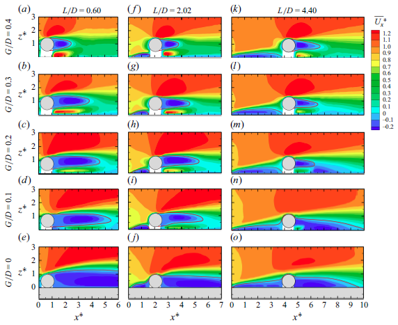
Figure 6 shows the time-averaged contours of
 $\overline{\mathit{U}_{\mathit{x}}^{\mathit{*}}}$
around a circular cylinder near the leading-edge separated flow of an elongated rectangular cylinder in the following cases: L / D = 0.60 and 0 ≤ G/D ≤ 0.4, L / D = 2.02 and 0 ≤ G/D ≤ 0.4 and L / D = 4.40 and 0 ≤ G/D ≤ 0.4. The behaviours of
 $\overline{\mathit{U}_{\mathit{x}}^{\mathit{*}}}$
are in good agreement with the smoke-wire flow visualisation results and can also be roughly categorised into three groups, supporting the validity of the present study.
Contours of
 $\overline{\mathit{U}_{\mathit{x}}^{\mathit{*}}}$
around the circular cylinder with L / D = 0.60 and 0 ≤ G/D ≤ 0.4, L / D = 2.02 and 0 ≤ G/D ≤ 0.4 and L / D = 4.40 and 0 ≤ G/D ≤ 0.4. Here,
 $\overline{\mathit{U}_{\mathit{x}}^{\mathit{*}}}$
is the normalised time-averaged velocity
 $\overline{\mathit{U}_{\mathit{x}}^{\mathit{*}}}\mathit{=}\overline{\mathit{U}_{\mathit{x}}}\mathit{/}\mathit{U}_{\mathit{\infty }}$
.

For classification I, as shown in figure 6(e), 6( j), 6(n) and 6(o), a large recirculation region, including a separation bubble on the leading edge of the rectangular cylinder and the near wake of the circular cylinder, dominates almost all the flow behaviours, as if the circular cylinder were a part of the rectangular cylinder. With an increase in L / D, the length and height of the near wake of the circular cylinder decrease from greater than 5D to 5D and from 1.1D to 0.7D, respectively, whereas the length of the separation bubble increases from less than 0.1D to 4D, as shown in figure 6(e), 6( j) and 6(o). In the gap between the circular and rectangular cylinders, the mean streamwise velocity
 $\overline{\mathit{U}_{\mathit{x}}^{\mathit{*}}}$
is negligible, although a region of positive
 $\overline{\mathit{U}_{\mathit{x}}^{\mathit{*}}}$
can be identified in the lower part of the near wake of the circular cylinder, which is covered by the wake recirculation region, as shown in figure 6(n). When 0 ≤ G/D ≤ 0.1, the scales of the circular cylinder near wake and leading-edge separation bubble both shrink noticeably.
For classification II, as shown in figure 6(b), 6(c), 6(d), 6(h), 6(i), 6(k), 6(l) and 6(m), the observed recirculation region clearly decays, and a gap flow characterised by a larger
 $\overline{\mathit{U}_{\mathit{x}}^{\mathit{*}}}$
than its surroundings is recognisable. With an increase in L / D, both the scales of the circular cylinder near wake and gap flow remarkably decrease. Taking figures 6(c), 6(h) and 6(m) as an example, the length and height of the circular cylinder near wake decrease from 4.5D to 1.5D and from 1.0D to 0.5D, respectively, and the maximum value of
 $\overline{\mathit{U}_{\mathit{x}}^{\mathit{*}}}$
in the gap flow reduces from 1.1 to 0.7. Moreover, in figure 6(c) and 6(h) , the lengths of the gap flow detected via
 $\overline{\mathit{U}_{\mathit{x}}^{\mathit{*}}}$
are approximately 3D and 2D, respectively, which are in fair agreement with the smoke-wire flow visualisation results as shown in figure 5(c). With an increase in G/D, the above observed leading-edge separation bubble noticeably decays and intensifies in the cases of L / D = 2.02 and 4.40, respectively, as shown in figure 6(h) and 6(i), and 6(k), 6(l) and 6(m), and the maximum value of
 $\overline{\mathit{U}_{\mathit{x}}^{\mathit{*}}}$
in the gap flow rises from 0.7 to 1.1.
For classification III, as shown in figure 6(a), 6( f) and 6(g), the circular cylinder near wake, leading-edge separation bubble and gap flow can be clearly recognised. The sizes of the circular cylinder near wake, the leading-edge separation bubble and the maximum value of
 $\overline{\mathit{U}_{\mathit{x}}^{\mathit{*}}}$
in the gap flow appear to reach saturation with varying L / D and G/D.
The trends for turbulent kinetic energy (TKE*),
 $\mathit{R}_{\mathit{uv}}^{\mathit{*}}$
and Q-criterion offer additional quantitative support for the flow features observed in smoke-wire flow visualisations and are consistent with the three classifications discussed earlier. The representative cases are shown in figures 7–9. The complete set of flow statistics (TKE*,
 $\mathit{R}_{\mathit{uv}}^{\mathit{*}}$
and Q) can be found in figures 23 ∼ 25 in the appendix.
Contours of
 $\mathit{TK}\mathit{E}^{\mathit{*}}$
around the circular cylinder;
 $TKE^*$
is the normalised turbulent kinetic energy
 $\mathit{TK}\mathit{E}^{\mathit{*}}\mathit{=}\mathit{TKE}\mathit{/}\mathit{U}_{\mathit{\infty }}^{\mathit{2}}$
. (a) Classification I (G/D = 0 and L / D = 2.02). (b) Classification II (G/D = 0.10 and L / D = 2.02). (c) Classification III (G/D = 0.40 and L / D = 2.02).

Contours of
 $\mathit{R}_{\mathit{uv}}^{\mathit{*}}$
around the circular cylinder. Here,
 $\mathit{R}_{\mathit{uv}}^{\mathit{*}}$
is the normalised Reynolds shear stress
 $\mathit{R}_{\mathit{uv}}^{\mathit{*}}=R_{uv}/U_{\infty }^{2}$
. (a) Classification I (G/D = 0 and L / D = 2.02). (b) Classification II (G/D = 0.10 and L / D = 2.02). (c) Classification III (G/D = 0.40 and L / D = 2.02).

Mean Q inline contours with the root-mean-square of the streamwise velocity fluctuation
 $u_{rms}^{*}$
. Vortical structures are indicated by the line contours of Q = 0.04
 $(\mathit{U}_{\mathit{\infty }}\mathit{/}\mathit{D})^{2}$
, with solid lines for clockwise motion and dashed lines for counterclockwise motion;
 $u_{rms}^{*}$
is normalised by the free-stream velocity
 $U_{\infty }$
. (a) Classification I (G/D = 0 and L / D = 2.02). (b) Classification II (G/D = 0.10 and L / D = 2.02). (c) Classification III (G/D = 0.40 and L / D = 2.02).

For classification I, as shown in figures 7(a), 8(a) and 9(a), large-scale turbulence structures featured by small TKE* and
 $\mathit{R}_{\mathit{uv}}^{\mathit{*}}$
and irregular vortices described by Q dominate the flow around the circular cylinder, and the values of TKE* and
 $\mathit{R}_{\mathit{uv}}^{\mathit{*}}$
near the gap between the circular and rectangular cylinders are negligible, except for the case shown in figure 24(n), which is as expected. As previously discussed in figure 6, this turbulence structure in the lower part of the circular cylinder near wake is situated within the wake recirculation region. More details can be found in figures 23(e), 23( j), 23(n) and 23(o), 24(e), 24( j), 24(n) and 24(o) and 25(e), 25( j), 25(n) and 25(o).
For classification II, as shown in figure 7(b), 8(b) and 9(b), large-scale turbulent structures can be detected in both the circular cylinder near wake and the gap flow, and the TKE* and
 $\mathit{R}_{\mathit{uv}}^{\mathit{*}}$
for these large-scale turbulent structures are both substantially higher. Meanwhile, the vortex structures exhibit more regularity. More importantly, a small-scale vortex characterised by elevated TKE* and
 $\mathit{R}_{\mathit{uv}}^{\mathit{*}}$
can be observed downstream of the gap flow. This vortex is near the circular cylinder and is expected to have a non-negligible effect on its aerodynamics. This effect will be discussed in the following section. More details can be found in figures 23(b), 23(c), 23(d), 23(h), 23(i), 23(k), 23(l) and 23(m), 24(b), 24(c), 24(d), 24(h), 24(i), 24(k), 24(l) and 24(m) and 25(b), 25(c), 25(d), 25(h), 25(i), 25(k), 25(l) and 25(m).
For classification III, as shown in figure 7(c), 8(c) and 9(c), large-scale turbulent structures are primarily observed in the circular cylinder near wake. Both the TKE* and
 $\mathit{R}_{\mathit{uv}}^{\mathit{*}}$
associated with these large-scale turbulent structures appear to have reached saturation. Additionally, a pair of well-defined vortices can be clearly identified within this region. More details can be found in figures 23(a), 23( f) and 23(g), 24(a), 24( f) and 24(g) and 25(a), 25( f) and 25(g).
Figure 10 presents the power spectral density (PSD) of the circular cylinder’s lift force, with the abscissa representing the non-dimensional frequency f* = fD/U ∞ . Two St values, i.e. St = 0.205 and 0.255, can be identified, corresponding to two distinct flow modes: an alternating vortex shedding mode and a one-sided shear flow mode, respectively. These flow modes were further revealed by applying POD method (2.9), with the results presented in figure 11. The POD reconstruction (2.10) was then employed to link these identified modes explicitly to the key flow characteristics embedded within the instantaneous flow field, as illustrated in figures 12 and 13.
Power spectral densities of lift force, for (a) L / D = 0.6, (b) L / D = 2.02 and (c) L / D = 4.4.

The
 $\omega ^{*}$
contours and velocity vectors of POD modes 1–4 with PSDs of the POD coefficients (
 $\mathit{a}_{\mathit{i}}$
), for (a) G/D = 0 and L / D = 0.60, (b) G/D = 0.20 and L / D = 0.60, (c) G/D = 0.30 and L / D = 0.60 and (d) an isolated circular cylinder.

(a)–(d) The
 $\omega$
reconstructions for the distorted alternating vortex shedding mode during one shedding cycle. (e)–(h) Snapshots during one shedding cycle.

(a)–(d) The
 $\omega$
reconstructions for the one-sided shear flow mode during one shedding cycle. (e)–(h) Snapshots during one shedding cycle.

The caseSt = 0.205 occurs when L / D = 0.6 (0.3 ≤ G/D ≤ 0.4), L / D = 2.02 (0.3 ≤ G/D ≤ 0.4) and L / D = 4.40 (G/D = 0.4). For an isolated circular cylinder, as shown in figure 11(d), the first four POD modes correspond to antisymmetric vortex shedding modes (the first and second modes) and symmetric vortex shedding modes (the third and fourth modes), respectively. The first two conjugate POD modes (1st: 25.34 % and 2nd: 24.10 %) indicate that the principal component of the field is alternating vortex shedding. While the vortex shedding mode becomes distorted due to the presence of the elongated rectangular cylinder, accompanied by a slight decrease in the energy contribution of the first two modes (1st: 22.09 % and 2nd: 21.89 %), as shown in figure 11(b). It is noteworthy that this distortion is more pronounced in the third and fourth POD modes. By reconstructing the flow behaviour of the first two POD modes, it can be observed that the flow exhibits a distorted alternating vortex shedding, with the shedding from the lower surface of the cylinder slightly suppressed, as shown in figure 12. Within one shedding cycle, the vortex shed from the lower surface dissipates rapidly in the wake, as illustrated in figure 12(c). In contrast, the upper-side vortex maintains a considerable size after shedding, with streamwise and transverse length of approximately 1.5D and 1.3D, respectively, as illustrated in figure 12(d). The distorted alternating vortex shedding can also be identified in the circular cylinder near wake, as illustrated in figure 14(c).
Typical flow patterns for the circular cylinder: (a) the one-sided shear flow mode (0 ≤ G/D ≤ 0.1), (b) the distorted one-sided shear flow mode (0.1 ≤G/D ≤ 0.2), (c) the distorted alternating vortex shedding mode (0.2 ≤ G/D ≤ 0.3) and (d) the alternating vortex shedding mode (0.3 ≤ G/D ≤ 0.4). The one-sided shear flow mode and the distorted one-sided shear flow mode have a dominant vortex shedding frequency of St ≈ 0.255, whereas the alternating vortex shedding mode and distorted alternating vortex shedding mode have a dominant vortex shedding frequency of St = 0.205.

The caseSt = 0.255 only occurs when L / D = 0.6 (0 ≤ G/D ≤ 0.2). In this situation, vortices shed solely from the upper side of the circular cylinder, whereas the shedding from the lower side is suppressed by the rectangular cylinder, as shown in figure 14(a). The upper-side shear layer has its own periodicity, but it is worth noting that this periodicity is relatively weak (figure 10 a). Figure 11(a) exhibits a POD mode pattern associated with one-side shedding, which distinctly differs from the alternating vortex shedding mode observed in figure 11(d). Furthermore, a one-sided shear flow can be distinctly observed in the reconstructed flow field, as illustrated in figure 13. The flow snapshots appear more chaotic because of the relatively low energy contribution of each POD mode (less than 10 %). As a result of the low modal energy content, the one-sided shear flow exhibits weak flapping during one cycle, resulting in the faint periodicity observed in the lift spectra.
In particular, the configuration with L / D = 0.6 (G/D = 0.2) can be considered a critical case, in which St ≈ 0.205 and 0.255 coexist (figure 10 a). The first two POD modes for L / D = 0.6 (G/D = 0.2) (figure 11 b) resemble those for L / D = 0.6 (G/D = 0.3) (figure 11 c), both representing a distorted alternating vortex shedding mode with further reduced energy contributions (1st: 18.34 % and 2nd: 17.83 %). Meanwhile, the third POD mode (figure 11 b) is similar to the first POD mode for L / D = 0.6 (G/D = 0) (figure 11 a), manifesting as a distorted one-sided shear flow mode. The coexistence of these flow modes results in the unique aerodynamic spectrum characteristics, featuring the coexistence of St ≈ 0.205 and 0.255.
For the distorted alternating vortex shedding mode, the lower surface shear layer of the circular cylinder and the leading-edge separated flow are deflected away from the rectangular cylinder. Rather than counteracting one another, these flow structures pair and merge, ultimately rolling up into a large-scale vortex (figure 14 c). This vortex interacts with those shed from the upper side of the circular cylinder and results in a St value of 0.180, below the value of 0.205 (figure 10 a). For the distorted one-sided shear flow mode, the counterclockwise vortices near the lower surface of the circular cylinder interact with the leading-edge separated flow of the rectangular cylinder, inducing the small-scale vortices (figure 14b ). The influence of the lower-surface vortices on the leading-edge separated flow is too weak to trigger alternating vortex shedding, thereby maintaining St = 0.255.
In figure 10(b) and 10(c), no dominant peaks are observed in the PSD of lift for both L / D = 2.02 and L / D = 4.40 under low G/D conditions. For L / D = 2.02 (G/D = 0) and L / D = 4.4 (G/D ≤ 0.1), the large-scale leading-edge separated flow overshoots the circular cylinder, dominating almost all the flow behaviours of the circular cylinder as if the circular cylinder were a part of the rectangular cylinder. There are no pronounced peaks in the lift spectrum since regular vortex shedding cannot be detected in this leading-edge separated flow at Re>2000 (Mills et al. Reference Mills, Sheridan and Hourigan2002, Reference Mills, Sheridan and Hourigan2003; Nakamura et al. Reference Nakamura, Ohya and Tsuruta1991). Moreover, for L / D = 2.02 (0.1 ≤ G/D ≤ 0.2) and L / D = 4.4 (0.2 ≤ G/D ≤ 0.3), the coherence of the shedding vortices is disrupted due to the interaction between the leading-edge separation bubble and the alternating shedding vortices.
3.3. Pressure distributions and aerodynamics classifications
Figures 15–17 presents the mean and fluctuating pressure coefficients
 $\overline{\mathit{C}_{\!\mathit{P}}}$
and
 $\mathit{C}_{\!\mathit{P}}^{\prime}$
around the circular cylinder for all 35 cases listed in figure 2(c). The pressure distributions of an isolated circular cylinder tested with the same set-up are also included in figures 15–17 as dashed lines for comparison. The pressure distributions are unfolded from the front stagnation point. The windward surface of the circular cylinder corresponds to θ values in the ranges 0–90° and 270–360°, whereas 0–180°, 90–270° and 180–360° are the upper, leeward and lower surfaces, respectively. In general, the
 $\overline{\mathit{C}_{\!\mathit{P}}}$
and
 $\mathit{C}_{\!\mathit{P}}^{\prime}$
of the currently investigated 35 cases are quite different from those of the isolated circular cylinder, indicating that the leading-edge separated flow substantially affects the pressure distributions around the circular cylinder. Further comparison reveals that the
 $\overline{\mathit{C}_{\!\mathit{P}}}$
and
 $\mathit{C}_{\!\mathit{P}}^{\prime}$
behaviours of these 35 cases can also be broadly grouped into three categories, which align well with both the smoke-wire flow visualisations and the PIV test results.
Distributions of
 $\overline{\mathit{C}_{\!\mathit{P}}}$
and
 $\mathit{C}_{\!\mathit{P}}^{\prime}$
on the circular cylinder above the elongated rectangular cylinder for classification I.

Distributions of
 $\overline{\mathit{C}_{\!\mathit{P}}}$
and
 $\mathit{C}_{\!\mathit{P}}^{\prime}$
on the circular cylinder above the elongated rectangular cylinder for classification II.

Distributions of
 $\overline{\mathit{C}_{\!\mathit{P}}}$
and
 $\mathit{C}_{\!\mathit{P}}^{\prime}$
on the circular cylinder above the elongated rectangular cylinder for classification III.

For classification I, as shown in figure 15, the following features are observed: a
 $\overline{\mathit{C}_{\!\mathit{P}}}$
< 0.6 on the front stagnation point, an almost constant
 $\overline{\mathit{C}_{\!\mathit{P}}}$
on the circular cylinder’s leeward surface and a smaller
 $\mathit{C}_{\!\mathit{P}}^{\prime}$
around the entire surface of the circular cylinder than in the isolated circular cylinder case. Moreover, the almost constant
 $\overline{\mathit{C}_{\!\mathit{P}}}$
transits from negative to positive at the intersection point of the circular and rectangular cylinders. However, with an increase in both L / D and G/D, new characteristics emerge in the pressure distribution; a
 $\overline{\mathit{C}_{\!\mathit{P}}}$
hump near θ ≈ 20° associated with a
 $\mathit{C}_{\!\mathit{P}}^{\prime}$
hump occurring at the corresponding position, some distortions of the almost constant
 $\overline{\mathit{C}_{\!\mathit{P}}}$
and an enhanced
 $\mathit{C}_{\!\mathit{P}}^{\prime}$
. Additionally, there is a gradual disappearance of the negative-to-positive transition in
 $\overline{\mathit{C}_{\!\mathit{P}}}$
at the intersection point of the two cylinders. The
 $\overline{\mathit{C}_{\!\mathit{P}}}$
and
 $\mathit{C}_{\!\mathit{P}}^{\prime}$
humps are likely caused by the previously identified intermittent reattachment of leading-edge separated flow shown in figure 5. The distortions in the otherwise constant
 $\overline{\mathit{C}_{\!\mathit{P}}}$
distribution can be attributed to both the above-mentioned intermittent reattachment and the turbulence structures within the near-wake recirculation region near θ ≈ 270° as shown in figures 23(n) and 24(n).
For classification II, as shown in figure 16, the previously discussed
 $\overline{\mathit{C}_{\!\mathit{P}}}$
and
 $\mathit{C}_{\!\mathit{P}}^{\prime}$
humps can still be identified, but they occur at θ ≈ 330° (the black and grey lines in figures 16
a and 16
b) on the lower surface of the circular cylinder. With an increase in L / D, the
 $\overline{\mathit{C}_{\!\mathit{P}}}$
and
 $\mathit{C}_{\!\mathit{P}}^{\prime}$
humps shift upwards to θ ≈ 10° (the red lines in figures 16
c and 16d), as expected. These pressure humps are likely caused by the previously observed reattachment of the leading-edge separated flow to the forebody of the circular cylinder. Another noteworthy phenomenon is the sudden intensification of
 $\mathit{C}_{\!\mathit{P}}^{\prime}$
, which reaches a maximum value of 0.17 at θ ≈ 270°. This can be detected for two specific cases: L / D = 2.02 and L / D = 1.60 when G/D = 0.6. In contrast, for the other cases, the
 $\mathit{C}_{\!\mathit{P}}^{\prime}$
remains within the expected range. This anomalous behaviour is likely caused by the previously identified small-scale, yet intense, vortex structure in the gap flow near the base of the circular cylinder, as shown in figures 7(i), 8(i) and 9(i).
For classification III, as shown in figure 17, the behaviour of
 $\overline{\mathit{C}_{\!\mathit{P}}}$
closely resembles that of an isolated circular cylinder, but it is asymmetric with respect to the nose–tail line, and this asymmetry is more pronounced for
 $\mathit{C}_{\!\mathit{P}}^{\prime}$
, whose value on the upper surface is smaller than on the lower surface. Compared with the isolated circular cylinder, the
 $\mathit{C}_{\!\mathit{P}}^{\prime}$
on the upper surface is consistently lower, indicating that the leading-edge separated flow has a mitigating effect on the alternating vortex shedding of the circular cylinder, even though the
 $\mathit{C}_{\!\mathit{P}}^{\prime}$
on the lower surface is in some cases larger than that of the isolated circular cylinder. These distortions in
 $\overline{\mathit{C}_{\!\mathit{P}}}$
and
 $\mathit{C}_{\!\mathit{P}}^{\prime}$
are primarily attributed to the interaction between the gap flow and the lower-side separated flow of the circular cylinder, as discussed above.
Based on the smoke-wire flow visualisations, quantitative PIV results and pressure distributions, the flow around a circular cylinder near the leading-edge separated flow of an elongated rectangular cylinder can be systematically categorised into three regimes: I (G/D = 0 and 0.60 ≤ L / D ≤ 5.80; G/D = 0.10 and 3.00 ≤ L / D ≤ 5.80), II (0.1 ≤ G/D ≤ 0.3 and L / D = 0.60; G/D = 0.1 and 1.60 ≤ L / D ≤ 2.02; G/D = 0.2 and 1.60 ≤ L / D ≤ 5.80; G/D = 0.30 and 3.00 ≤ L / D ≤ 5.80; G/D = 0.40 and 4.40 ≤ L / D ≤ 5.80) and III (G/D = 0.3 and 1.60 ≤ L / D ≤ 3.00; G/D = 0.40 and 0.60 ≤ L / D ≤ 3.56), as shown in figure 18. For regime I, the circular cylinder can be regarded as part of the rectangular cylinder, leading to its designation as the ‘broadened-body regime’. For regime II, the leading-edge separated flow fully reattaches to the forebody of the circular cylinder, therefore, it is referred to as the ‘body-reattachment regime’. For regime III, both the leading-edge separated flow and von Kármán vortex shedding can be observed, as well as their interaction, therefore, it is termed the ‘co-shedding regime’.
Distribution patterns of the circular-rectangular cylinder with variations in L / D and G/D., including three primary regimes: I: broadened body, II: body reattachment and III: co-shedding, respectively. The blue, red, half-blue and half-red and white points represent the vortex shedding mode, the shear layer mode, the combined impact of both and the absence of a dominant frequency, respectively.

The vortex shedding characteristics of the circular cylinder are also illustrated in figure 18 through four styles of coloured markers: blue, red, half blue and half red and white. Blue corresponds to the alternating vortex shedding mode (St = 0.205) referenced in figure 10, occurring in regimes III and II (L / D = 0.6 and G/D ≥ 0.20; 4.40 ≤ L / D ≤ 5.80 and G/D ≥ 0.40). The red point represents the one-sided shear flow mode (St = 0.255), observed in regimes I (L / D = 0.60 and G/D = 0) and II (L / D = 0.60 and 0.10 ≤ G/D ≤ 0.30). Notably, in regime II (L / D = 0.60 and 0.20 ≤ G/D ≤ 0.30), both the vortex shedding mode (St = 0.205) and the one-sided shear flow mode (St = 0.255) coexist, as indicated by the half-blue, half-red circles of figure 18. At the white points, no significant dominant frequency is observed.
As the position of the circular cylinder changes relative to the rectangular cylinder, some aerodynamic characteristics of individual regimes inevitably begin to resemble those of others. This is due to the nonlinear correspondence between fluid dynamics and aerodynamics. Additionally, the flow structures that initially dominated in this regime weaken, while flow structures predominate in other regimes, such as separation flow, gap flow or the recirculation region, become increasingly influential as L / D and G/D vary. Moreover, for cylinders that exhibit periodic lift, beyond the dominant flow mode in each regime, they are also influenced by the flow modes. Consequently, a certain degree of convergence of different flow regimes is inevitable.
3.4. Aerodynamic forces
The aerodynamic coefficients of the circular cylinder are obtained by integrating and statistically analysing the pressure on its surface, as shown in figure 19, in which the black lines represent the boundaries between the three distinct flow regimes. It is not difficult to observe that the distribution of the aerodynamic force coefficients of the circular cylinder with respect to L / D and G/D correlate with the classified flow regimes, although the degree of correlation varies across different force components. However, as with the macroscopic statistical quantities, the aerodynamic force coefficients may not capture all the complexities of the underlying flow structures, and their nonlinear relationship can lead to discrepancies between the force measurements and detailed flow behaviours.
Aerodynamic forces of the circular cylinder above the elongated rectangular cylinder at different L / D and G/D: (a)
 $\overline{\mathit{C}_{\!\mathit{D}}}$
, (b)
 $\mathit{C}_{\!\mathit{D}}^{\prime}$
, (c)
 $\overline{\mathit{C}_{\mathit{L}}}$
and (d)
 $\mathit{C}_{\!\mathit{L}}^{\prime}$
.

The bottom region corresponds to regime I, as a part of the elongated rectangular cylinder, the circular cylinder experiences conditions of direct attachment (bottom left) and coverage by separated flow (bottom right) under the influence of the incoming flow, corresponding to the large and small
 $\overline{\mathit{C}_{\!\mathit{D}}}$
, respectively, as shown in figure 19(a). Meanwhile, the stable attachment of the airflow effectively reduces
 $\mathit{C}_{\!\mathit{D}}^{\prime}$
(figure 19
b). However, as L / D increases,
 $\mathit{C}_{\!\mathit{D}}^{\prime}$
becomes significantly larger because of the intermittent impingement of the leading-edge separated flow onto the windward side of the cylinder. It is noteworthy that, in regime I (figure 19
b), the cylinder at the critical state of
 $\mathit{C}_{\!\mathit{D}}^{\prime}$
(3 ≤ L / D ≤ 4) exhibits lower
 $\overline{\mathit{C}_{\!\mathit{D}}}$
(figure 19
a), indicating that the cylinder is largely covered by the leading-edge separated flow at this stage. Under more downstream conditions (L / D ≥ 4), the influence of the leading-edge separated flow on the cylinders weakens. Compared with the critical state (3 ≤ L / D ≤ 4), the intermittent reattachment of the airflow leads to high
 $\overline{\mathit{C}_{\!\mathit{D}}}$
and
 $\mathit{C}_{\!\mathit{D}}^{\prime}$
. Under the influence of the incoming flow and separated flow, the upper-side pressure taps of the circular cylinder exhibit negative
 $\overline{\mathit{C}_{\!\mathit{P}}}$
(figure 15
a–c) and results in a positive
 $\overline{\mathit{C}_{\mathit{L}}}$
(figure 19
c). Moreover, regardless of whether the airflow is stably directly attached, its impact on the pressure fluctuations on the cylinder surface is quite limited, thereby leading to lower
 $\mathit{C}_{\mathit{L}}^{\prime}$
(figure 19
d).
The central contour represents regime II, in which the separated flow at the leading edge of the rectangular cylinder directly interacts with the flow around it. Meanwhile, complex flow structures such as gap flow, gap vortices and the recirculation zone are generated. Regime II is predominantly influenced by the attachment of the incoming flow, exhibiting a relatively large
 $\overline{\mathit{C}_{\!\mathit{D}}}$
(figure 19
a). According to the results from the flow visualisation (figure 5
b–d), the left contour of this regime (L / D = 0.6) indicates that the circular cylinder is almost directly enveloped by the incoming flow. Its lower surface is slightly influenced by the leading-edge separated flow, but the effects of the recirculation zone and gap flow are limited. As a result, the fluctuating wind pressure is relatively small (figure 19
b). For the cylinder located further downstream (3 ≤ L / D ≤ 5.8), the recirculation zone at the leading edge is fully developed, resulting in pronounced
 $\mathit{C}_{\!\mathit{D}}^{\prime}$
(figure 19
b) and
 $\mathit{C}_{\mathit{L}}^{\prime}$
(figure 19
d). As a result of the pumping action within the recirculation zone, an increased flow is effectively directed into the gap, resulting in the lower surface of the cylinder experiencing suction due to negative pressure, which manifests as negative
 $\overline{\mathit{C}_{\mathit{L}}}$
(figure 19
c). Additionally, the presence of the recirculation zone partially mitigates the impact of the incoming flow, leading to a reduction in
 $\overline{\mathit{C}_{\!\mathit{D}}}$
, as illustrated in (figure 19
a) (G/D = 0.2 and 3 ≤ L / D ≤ 5.8). This condition persists until G/D = 0.3 and 0.4.
The top contour corresponds to regime III, in which the coupling effect between the flow around the cylinder and the separated flow at the leading edge of the elongated rectangular cylinder weakens. This increases the similarity to the isolated cylinder case, with the
 $\overline{\mathit{C}_{\mathit{L}}}$
of the cylinder approaching zero (figure 19
c). Under the influence of alternating vortex shedding, it exhibits significant
 $\mathit{C}_{\!\mathit{D}}^{\prime}$
(figure 19
b) and
 $\mathit{C}_{\mathit{L}}^{\prime}$
(figure 19
d). Additionally, due to the direct attachment of the airflow, the cylinder has a large
 $\overline{\mathit{C}_{\!\mathit{D}}}$
(figure 19
a).
Overall, the distributions of aerodynamic force coefficients of the circular cylinder with respect to G/D and L / D align to some extent with the flow regimes, as seen in
 $\overline{\mathit{C}_{\!\mathit{D}}}$
(figure 19
a). The discrepancies between them arise because complex flow patterns cannot be fully captured by macroscopic statistics, as mentioned earlier, and because of variations in specific details of the flow. Two representative cases are discussed here.
Distributions of
 $\overline{\mathit{C}_{\!\mathit{p}}}$
and
 $\mathit{C}_{\!\mathit{p}}^{\prime}$
on the circular cylinder above the elongated rectangular cylinder at different Reynolds numbers (Re = 40,000, 60,000, 80,000, and 100,000) for G/D = 0.2 and L / D = 0.6.

Contours of mean streamwise velocity
 $\overline{U_{x}^{\mathrm{*}}}$
and turbulent kinetic energy TKE* around an elongated rectangular cylinder at different Reynolds numbers (Re = 40,000, 60,000, 80,000 and 100,000). (a)–(d) Mean streamwise velocity. (e)–(h) Turbulent kinetic energy.

Aerodynamic forces exhibit some variation even within the same flow regime. As shown in regime II of figure 19(c), the reattachment of the leading-edge separated flow governs the flow behaviours and influences the aerodynamic characteristics. However, the positions of reattachment differ, leading to variations in aerodynamic forces. For 0.60 ≤ L / D ≤ 1.60, the previously discussed
 $\overline{\mathit{C}_{\!\mathit{P}}}$
hump is observed at θ ≈ 330° (the black and grey lines in figure 16
a), suggesting flow reattachment on the lower windward side of the circular cylinder. For 3.00 ≤ L / D ≤ 5.80, the
 $\overline{\mathit{C}_{\!\mathit{P}}}$
hump shifts upwards to θ ≈ 10° (the red lines in figure 16
c), and the absolute value of negative pressure on the upper windward side (near θ ≈ 60°) is lower than that of an isolated cylinder, indicating that reattachment occurs on the upper windward surface. The range of 1.60 ≤ L / D ≤ 3.00 represents a transitional state between these two configurations. These phenomena are also corroborated by flow visualisation results (including the smoke-wire visualisation in figure 5, the supplemental multimedia and additional flow statistics in the appendix). Furthermore, for 3.00 ≤ L / D ≤5.80, the intermittent reattachment of the leading-edge separated flow observed through flow visualisation leads to larger fluctuation amplitudes than in the case of 0.60 ≤ L / D ≤ 1.60, as shown in regime II of figure 19(b) and 19(d). Despite the differences in aerodynamic characteristics caused by variations in flow details (such as reattachment location and intermittent reattachment), the fundamental nature of the leading-edge separated flow reattachment remains consistent. Therefore, these cases belong to the body-reattachment regime.
Aerodynamic forces may also exhibit similar magnitudes across different flow regimes. As shown in figures 19(b) and 19(d), comparable magnitudes of
 $\mathit{C}_{\!\mathit{D}}^{\prime}$
(or
 $\mathit{C}_{\mathit{L}}^{\prime}$
) are observed in the right portion of regime II and throughout regime III, but the underlying flow mechanisms differ. In regime II, this effect is caused by the intermittent reattachment of leading-edge separation flow, whereas regime III is characterised by alternating vortex shedding. Therefore, they cannot be classified under the same flow regime although their force magnitudes might be similar.
Contours of mean streamwise velocity
 $\overline{U_{x}^{\mathrm{*}}}$
and turbulent kinetic energy TKE* for L / D = 0.6 and G/D = 0.2 at different Reynolds numbers (Re = 40,000, 60,000, 80,000 and 100,000). (a)–(d) Mean streamwise velocity. (e)–(h) Turbulent kinetic energy.

Contours of
 $\mathit{TK}\mathit{E}^{\mathit{*}}$
around the circular cylinder for L / D = 0.60, 2.02 and 4.40 and 0 ≤ G/D ≤ 0.4. Here,
 $\mathit{TK}\mathit{E}^{\mathit{*}}$
is the normalised turbulent kinetic energy
 $\mathit{TK}\mathit{E}^{\mathit{*}}\mathit{=}\mathit{TKE}\mathit{/}\mathit{U}_{\mathit{\infty }}^{\mathit{2}}$
.

Contours of
 $\mathit{R}_{\mathit{uv}}^{\mathit{*}}$
around the circular cylinder for L / D = 0.60, 2.02 and 4.40 and 0 ≤ G/D ≤ 0.4. Here,
 $\mathit{R}_{\mathit{uv}}^{\mathit{*}}$
is the normalised Reynolds shear stress
 $\mathit{R}_{\mathit{uv}}^{\mathit{*}}=R_{uv}/U_{\infty }^{2}$
.

Mean Q inline contours with the root-mean-square of the streamwise velocity fluctuation
 $u_{rms}^{*}$
for L / D = 0.60, 2.02 and 4.40 and 0 ≤ G/D ≤ 0.4. Vortical structures are demonstrated by the line contours of Q = 0.04
 $(\mathit{U}_{\mathit{\infty }}\mathit{/}\mathit{D})^{2}$
, with solid lines for clockwise motion, and dashed lines for counterclockwise motion. Here,
 $u_{rms}^{*}$
is normalised by the free-stream velocity
 $U_{\infty }$
.

4. Concluding remarks
This experimental study examined the aerodynamic and flow characteristics of a circular cylinder near the leading-edge separated flow of an elongated rectangular cylinder with varying gap-to-diameter ratio (G/D) of 0 ≤ G/D ≤ 0.4 and a distance-to-diameter ratio (L / D) of 0.6 ≤ G/D ≤ 5.8. Smoke-wire flow visualisations, PIV test results, lift power spectral densities and pressure distributions were used in the analysis. Three different flow regimes of the circular cylinder were identified, i.e. the broadened-body, body-reattachment and co-shedding regimes, each corresponding to distinct flow structures and dynamic properties, as summarised below.
In the broadened-body regime (G/D = 0, 0.60 ≤ L / D ≤ 5.80 and G/D = 0.10, 3.00 ≤ L / D ≤ 5.80), almost no gap flow can be identified and the leading-edge separated flow overshoots the circular cylinder, which results in a small
 $\mathit{C}_{\mathit{L}}^{\prime}$
and a large
 $\overline{\mathit{C}_{\mathit{L}}}$
for the circular cylinder. For G/D = 0 and L / D = 0.60, the lower body of the circular cylinder has an almost constant
 $\overline{\mathit{C}_{\!\mathit{P}}}$
, which transitions from negative to positive at the intersection point of the circular cylinder and the rectangular cylinder, and a
 $\mathit{C}_{\!\mathit{P}}^{\prime}$
approaching zero. For G/D = 0 and 1.60 ≤ L / D ≤ 5.80, an almost constant
 $\overline{\mathit{C}_{\!\mathit{P}}}$
around the lower body of the circular cylinder can still be identified, whereas a
 $\mathit{C}_{\!\mathit{P}}$
hump occurs near the front stagnation of the circular cylinder which is caused by the intermittent reattachment of the leading-edge separated flow, as well as a strengthened
 $\mathit{C}_{\!\mathit{P}}^{\prime}$
. For G/D = 0.10 and 3.00 ≤ L / D ≤ 5.80, the
 $\overline{\mathit{C}_{\!\mathit{P}}}$
hump can also be recognised, whereas the almost constant
 $\overline{\mathit{C}_{\!\mathit{P}}}$
gradually fades.
In the body-reattachment regime (G/D = 0.10, 0.60 ≤ L / D ≤ 2.02; G/D = 0.20, 0.60 ≤ L / D ≤ 5.80; G/D = 0.30, L / D = 0.60 and 3.00 ≤ L / D ≤ 5.80; and G/D = 0.40, 4.40 ≤ L / D ≤ 5.80), gap flow is discernible, and the leading-edge separated flow fully reattaches to the forebody of the circular cylinder, which causes a significantly reduced
 $\overline{\mathit{C}_{\mathit{L}}}$
and the disappearance of the almost constant
 $\overline{\mathit{C}_{\!\mathit{P}}}$
, compared with the broadened-body regime. The
 $\overline{\mathit{C}_{\!\mathit{P}}}$
hump experiences a progressive rearward shift due to the rearward movement of the reattachment point of the leading-edge separated flow. This is associated with a significantly enhanced
 $\mathit{C}_{\!\mathit{P}}^{\prime}$
and a negative
 $\overline{\mathit{C}_{\!\mathit{P}}}$
around the lower body of the circular cylinder because of the strengthening gap flow and recirculation zone. Most notably, two Strouhal numbers, i.e. St = 0.205 and 0.255, are detected. The former is attributed to the vortices alternately shed from the upper and lower sides of the circular cylinder, whereas the latter arises from the vortices shedding only from the upper side of the circular cylinder.
In the co-shedding regime (G/D = 0.30, 1.60 ≤ L / D ≤ 2.02 and G/D = 0.40, 0.60 ≤ L / D ≤ 3.56), gap flow can be clearly discerned, and the leading-edge separated flow remarkably alters the vortex shedding from the lower side of the circular cylinder without reattachment, resulting in distorted alternate vortex shedding from the circular cylinder and significantly increased
 $\overline{\mathit{C}_{\!\mathit{D}}}$
,
 $\mathit{C}_{\!\mathit{D}}^{\prime}$
and
 $\mathit{C}_{\mathit{L}}^{\prime}$
. The
 $\overline{\mathit{C}_{\!\mathit{P}}}$
hump and constant
 $\overline{\mathit{C}_{\!\mathit{P}}}$
observed in the body-reattachment regime almost disappear as G/D and L / D increase, and
 $\overline{\mathit{C}_{\!\mathit{P}}}$
and
 $\mathit{C}_{\!\mathit{P}}^{\prime}$
closely resemble those of an isolated circular cylinder, while the
 $\mathit{C}_{\!\mathit{P}}^{\prime}$
distribution is asymmetric with respect to the nose–tail line because of the distorted alternating vortex shedding.
This study focuses on the flow field and aerodynamic forces around a circular cylinder positioned near a rectangular cylinder, it does not account for certain factors. These include the height of the rectangular cylinder and its corner geometry, which may influence separated flow patterns and consequently affect the dimensions of separation bubbles. These parameters will be systematically examined in future work to quantify their specific impacts.
Supplementary movies
Supplementary movies are available at https://doi.org/10.1017/jfm.2025.10991.
Acknowledgements
The supports from the National Natural Science Foundations of China (Grant Nos. 52327810 and 52208514), the Natural Science Foundation of Hunan province (Grant No. 2024JJ4063) and the Hunan Province Innovation Research Group Project (Grant No. 2025JJ10005) are gratefully acknowledged.
Data availability
Data will be made available on request.
Author contributions
Yage Wu: Conceptualisation, Data curation, Formal analysis, Funding acquisition, Investigation, Software, Validation, Writing – original draft, Writing – review and editing. Huan Li: Data curation, Investigation, Software, Writing – original draft. Xuhui He: Conceptualisation, Funding acquisition, Writing – review and editing. Jing Zhu: Conceptualisation, Investigation, Writing – review & editing. Hanfeng Wang: Conceptualisation, Funding acquisition, Writing – review and editing. Bingfu Zhang: Conceptualisation, Investigation, Writing – review.
Declaration of interest
The author(s) report no conflict of interest.
Appendix. Flow statistics
This appendix presents a comparative analysis of the effect of Reynolds number, using the configuration with L / D = 0.6 and G/D = 0.2 as a representative case, as illustrated in Figures 20∼22.
Furthermore, the time-averaged contours of TKE*,
 $\mathit{R}_{\mathit{uv}}^{\mathit{*}}$
, and Q around the circular cylinder near the leading-edge separated flow of an elongated rectangular cylinder for the cases of L / D = 0.60, 2.02, 4.40 and 0 ≤ G/D ≤ 0.4, are illustrated in figures 23∼25.