1 Introduction
Although turbulence is pervasive in natural and industrial fluid flows, providing a precise and universally agreed-upon definition for this flow state remains an open challenge. Nevertheless, most fluid dynamicists would agree that a large separation between the scales at which the flow is driven and the scales at which the energy is dissipated and an associated cascade of energy between the two are necessary conditions to describe a flow as turbulent (Falkovich Reference Falkovich2009). Because of the scale separation between driving and dissipation, energy is nearly conserved in the cascade, leading to a presumed scale invariance and universality in this ‘inertial’ range. Consequently, characterization and prediction of the behaviour of various statistical quantities in the inertial range has tended to dominate fundamental research in turbulence.
This kind of statistical approach, however, somewhat downplays the detailed mechanisms responsible for the cascade itself. At a high level, the cascade certainly arises from the wavevector triad interactions present in the nonlinear term in the Navier–Stokes equations that couple different scales; but the Navier–Stokes equations alone do not illuminate the details of the spectral energy transfer, nor why some wavevector couplings (such as those that are local in scale) are preferentially selected (Batchelor Reference Batchelor1953).
Here, we suggest that a more mechanical perspective may serve to illuminate the details of the energy cascade more clearly. As with any energy transfer process, the energy flux in the turbulent cascade can be cast as the result of the interplay between a stress and a rate of strain. At a given scale in the cascade, the relevant strain rate is that of the flow at that scale. The necessary stress arises from the nonlinear term in the Navier–Stokes equations as a consequence of the scale restriction of the turbulence, as occurs in, for example, Reynolds averaging or large-eddy simulation (Pope Reference Pope2000). In this formulation, the energy cascade can be interpreted as the effect of some scales doing net mechanical work on others (Chen et al. Reference Chen, Ecke, Eyink, Rivera, Wan and Xiao2006; Fang & Ouellette Reference Fang and Ouellette2016). In three-dimensional (3-D) turbulence, for example, it is the large scales that work on the small scales, as is evident in the direction of the cascade; in two dimensions, where the cascade reverses direction, it is the opposite. The rate at which this work is done is captured by the inner product of the turbulent stress and the strain rate.
In this formulation, it then immediately becomes clear that the relative geometry of these two tensors is key to understanding the cascade: for the same tensor magnitudes, the energy flux can be forward (if the tensors are aligned), inverse (if they are anti-aligned) or vanishing (if they are orthogonal). Since all turbulent flows display a cascade, one would therefore expect strong alignment between these tensors; but in both 2-D and 3-D turbulence, it is well known that the alignment is surprisingly weak (Wallace Reference Wallace2009). Thus, in a sense that we will make precise in § 4, the cascade can be interpreted as a relatively inefficient process (Fang & Ouellette Reference Fang and Ouellette2016).
Because geometric alignment plays a fundamental role in the cascade, it has been studied for quite some time in turbulence. In 3-D turbulence, the alignment between the strain-rate eigenvectors and the vorticity vector is most commonly investigated (Borue & Orszag Reference Borue and Orszag1998), since vortex stretching is often taken to be the mechanism that produces the energy cascade (Taylor Reference Taylor1932, Reference Taylor1938; Tennekes & Lumley Reference Tennekes and Lumley1972). The transfer of energy from large to small scales is strongest when the vorticity vector points in the direction of the most extensional eigenvector of the strain rate. As has been found in many studies, however, in real turbulence the vorticity is on average instantaneously aligned with the strain-rate eigenvector corresponding to the intermediate eigenvalue instead (Ashurst et al. Reference Ashurst, Kerstein, Kerr and Gibson1987; Tsinober, Kit & Dracos Reference Tsinober, Kit and Dracos1992; Vincent & Meneguzzi Reference Vincent and Meneguzzi1994; Ni et al. Reference Ni, Kramel, Ouellette and Voth2015). This intermediate eigenvalue does tend to be weakly extensional (Betchov Reference Betchov1956; Ashurst et al. Reference Ashurst, Kerstein, Kerr and Gibson1987), so that the net energy cascade is still from large to small scales, but the lack of alignment with the strongest extensional eigenvector has often been construed as being somewhat mysterious.
Less work has been done on studying the alignment between the actual turbulent stress and the strain rate in 3-D turbulence, in part because the scale-dependent stress is more difficult to extract than the vorticity. Nevertheless, some measurements have been made using filtering techniques similar to those we will employ below (Tao, Katz & Meneveau Reference Tao, Katz and Meneveau2000, Reference Tao, Katz and Meneveau2002; Higgins, Palange & Meneveau Reference Higgins, Palange and Meneveau2003; Higgins, Meneveau & Palange Reference Higgins, Meneveau and Palange2007). Analogously to what was found for the vorticity and the strain rate, the stress was found to be misaligned from the strain rate by a fairly significant margin (Tao et al. Reference Tao, Katz and Meneveau2000, Reference Tao, Katz and Meneveau2002), in contrast to what is assumed in typical eddy viscosity or Smagorinsky models (Pope Reference Pope2000).
Because the case of 2-D turbulence is geometrically simpler and because vortex stretching plays no role in the 2-D inverse cascade (since the vortex stretching term is identically zero in two dimensions), investigations of the alignment between the stress and the strain rate have a somewhat longer history in 2-D turbulence. The general conclusion, however, is the same as in three dimensions: the stress and the strain are on average highly misaligned (Chen et al. Reference Chen, Ecke, Eyink, Rivera, Wan and Xiao2006; Xiao et al. Reference Xiao, Wan, Chen and Eyink2009; Liao & Ouellette Reference Liao and Ouellette2014, Reference Liao and Ouellette2015; Fang & Ouellette Reference Fang and Ouellette2016).
Here, we consider the geometric alignment between the turbulent stress and the rate of strain in detail. In § 2, we make explicit the role this alignment plays in the mechanics of the energy cascade. Then, in § 3 we formulate this alignment in terms of Euler angles to make clear the contribution of both the eigenvalues of these two tensors and the orientation of their eigenvectors. In particular, we show that the eigenvalues are necessary to describe the alignment in three dimensions, but that in two dimensions the tensor alignment depends only on the orientations of the eigenvectors. In § 4, we follow our previous work (Fang & Ouellette Reference Fang and Ouellette2016) to define a notion of an efficiency in the cascade, which behaves very differently in two and three dimensions. Finally, in § 5, we make our general results specific to turbulence by computing tensor geometry and efficiencies using the direct numerical simulation of homogeneous, isotropic turbulence available from the Johns Hopkins Turbulence Database (Li et al. Reference Li, Perlman, Wan, Yang, Meneveau, Burns, Chen, Szalay and Eyink2008).
2 Mechanical formulation of the scale-to-scale energy flux
As can be seen directly by considering them in Fourier space, the nonlinear term in the Navier–Stokes equations leads to the coupling of different scales of motion. When the Reynolds number is large, the nonlinearity dominates the dynamics and these scale couplings are highly active. This observation, in conjunction with the broadband energy spectrum that is typical of turbulent flows, leads to a phenomenological picture of turbulence along the lines of the classical Richardson–Kolmogorov energy cascade. In this kind of description, we think of ‘eddies’ with well-defined spatial and temporal scales that break up into smaller eddies, transferring their energy and momentum to smaller scales by virtue of this breakup process. These eddies, however, are typically defined somewhat loosely, and should not be construed to be, for example, vortices; rather, they are best understood only as those degrees of freedom that remain in the flow field after some kind of bandpass filtering in scale space (Frisch Reference Frisch1995). Thus, although they are useful for conceptually illustrating the idea of the energy cascade, it is not clear how to build a precise, mechanistic model from Richardson eddies.
The coupling between scales that is inherent in the nonlinear term also has a signature in physical space, however, that is easier to interpret physically. As is well known, removing any of the degrees of freedom in a flow will result in the appearance of a source or sink of momentum or energy for the degrees of freedom that are retained. In turbulence, this kind of dimensionality reduction appears most commonly in Reynolds averaging to isolate the mean flow or in filtering to retain only the large eddies (Pope Reference Pope2000). After applying either averaging or filtering, the new momentum equation for the retained field acquires a term that looks like the divergence of a stress, and the new energy equation has an additional term that is a source or sink of energy.
The quadratic nature of the nonlinearity in the Navier–Stokes equations constrains the form of these new terms. Thus, the application of any linear operator
 ${\mathcal{P}}$
that projects the full dynamics onto a subspace with a restricted number of degrees of freedom will lead to a new turbulent stress, which we denote as
 $\tilde{\unicode[STIX]{x1D70F}}_{ij}$
and define as
 $$\begin{eqnarray}\tilde{\unicode[STIX]{x1D70F}}_{ij}={\mathcal{P}}(u_{i}u_{j})-{\mathcal{P}}(u_{i}){\mathcal{P}}(u_{j}).\end{eqnarray}$$
 ${\mathcal{P}}$
is most commonly taken to be an averaging or filtering operator, but it need not be; the mathematical results that follow are independent of the precise form of
 ${\mathcal{P}}$
. We interpret
 $\tilde{\unicode[STIX]{x1D70F}}_{ij}$
as a stress because it enters the momentum equation for the projected field
 ${\mathcal{P}}(u_{i})=\tilde{u} _{i}$
in the divergence
 $\unicode[STIX]{x2202}\tilde{\unicode[STIX]{x1D70F}}_{ij}/\unicode[STIX]{x2202}x_{j}$
, where summation is implied over repeated indices. Thus, it encodes the momentum coupling between the retained and removed degrees of freedom. Consistently, the new term in the equation of motion for the projected kinetic energy
 $\tilde{E}=(1/2)\tilde{u} _{i}\tilde{u} _{i}$
has the form
 $$\begin{eqnarray}-\tilde{\unicode[STIX]{x1D70F}}_{ij}\tilde{\unicode[STIX]{x1D634}}_{ij}=\tilde{\unicode[STIX]{x1D6F1}},\end{eqnarray}$$
where
 $\tilde{\unicode[STIX]{x1D634}}_{ij}=(1/2)(\unicode[STIX]{x2202}\tilde{u} _{i}/\unicode[STIX]{x2202}x_{j}+\unicode[STIX]{x2202}\tilde{u} _{j}/\unicode[STIX]{x2202}x_{i})$
is the rate of strain of the projected field.
 $\tilde{\unicode[STIX]{x1D6F1}}$
gives the rate of energy transfer between the retained and removed degrees of freedom, and we refer to it as the spectral energy flux. In principle,
 $\tilde{\unicode[STIX]{x1D6F1}}$
expresses the energy transferred between all of the retained and removed degrees of freedom. Given the nature of turbulence, however, one can estimate the scales that dominantly contribute to
 $\tilde{\unicode[STIX]{x1D6F1}}$
. Since the velocity magnitude must be bounded, the dominant contribution to the velocity gradient will come from the smallest length scales; thus,
 $\tilde{\unicode[STIX]{x1D634}}_{ij}$
can be viewed as characterizing the smallest length scales in the retained velocity field. In both two and three dimensions, most of the kinetic energy in turbulent flows resides at the largest scales (due to energy injection in three dimensions and inverse cascade in two dimensions); thus, the dominant contribution to
 $\tilde{\unicode[STIX]{x1D70F}}_{ij}$
, which depends on the velocity alone with no derivatives, comes from the largest scales of the removed velocity field. Thus, if we choose
 ${\mathcal{P}}$
to be a projection operation that removes scales smaller than some cutoff, as we will below,
 $\tilde{\unicode[STIX]{x1D6F1}}$
is approximately localized in scale at this cutoff.
In one sense, this formulation is just as abstract as that of the coupling of wavevectors in a Fourier description of the cascade or the breakup of eddies in the Richardson–Kolmogorov picture, because the stress defined in (2.1) is a rather strange quantity. But by writing the coupling between scales in terms of this stress, we gain the advantage of describing the energy transfer as a purely mechanical process. Now, instead of picturing the abstract breakup of eddies that are themselves ill defined, we can think of the cascade as emerging from the net tendency of some scales to do mechanical work on others, as encapsulated in this turbulent stress. For example, in 3-D turbulence, the cascade must result from degrees of freedom with large spatio-temporal scales doing work on those with small spatio-temporal scales. This interpretation also frees us from ever having to define Richardson eddies in a precise fashion.
Working in this framework also immediately makes it clear that we cannot ignore the geometry of the stress and the strain rate. Following from both mathematical and physical arguments, the relative orientation of the eigenframes of these two tensors is key for characterizing the energy cascade. Mathematically, as shown in (2.2), the spectral energy flux
 $\tilde{\unicode[STIX]{x1D6F1}}$
is given as the inner product of the stress and the strain rate. Just as for the more familiar case of vectors, the value of this inner product between second-rank tensors can be suppressed if their eigenframes are misaligned. Physically, transferring energy from one system to another – in this case, between the retained field and the removed field – means that work must be done. But even given finite force and displacement (generalized here to stress and strain), work is only done if the force acts in the direction of the displacement. If the stress and strain rate are misaligned, no work will be done, and the cascade will not occur. Thus, formulating the energy cascade in these mechanical terms allows us to apply mechanical intuition to understand the kinds of scale interactions that must occur to generate it.
3 Tensor geometry via Euler angles
As introduced in § 2, the energy flux between scales
 $\tilde{\unicode[STIX]{x1D6F1}}$
can be written as the inner product of the turbulent stress
 $\tilde{\unicode[STIX]{x1D70F}}_{ij}$
and the rate of strain
 $\tilde{\unicode[STIX]{x1D634}}_{ij}$
. The rate of strain is symmetric and deviatoric in incompressible flow. The stress is symmetric, but is not in general deviatoric; however, we can neglect the trace of the stress because it does not impact this inner product (Xiao et al.
Reference Xiao, Wan, Chen and Eyink2009; Liao & Ouellette Reference Liao and Ouellette2015). Thus, we can consider each of these tensors to be symmetric and deviatoric in our analysis.
3.1 Two-dimensional alignment
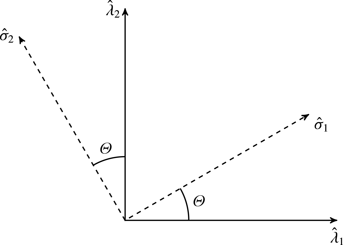
Sketch of the eigenframes of the stress and the strain rate in two dimensions.
 $\hat{\unicode[STIX]{x1D706}}_{1}$
and
 $\hat{\unicode[STIX]{x1D706}}_{2}$
are the extensional and compressional eigenvectors, respectively, of the stress, and
 $\hat{\unicode[STIX]{x1D70E}}_{1}$
and
 $\hat{\unicode[STIX]{x1D70E}}_{2}$
are the corresponding eigenvectors of the strain rate. Each pair of corresponding stress and strain-rate eigenvectors are separated by an angle
 $\unicode[STIX]{x1D6E9}$
.

To build intuition for how the alignment of the eigenframes of these two tensors impacts the scale-to-scale energy flux, we first consider them in 2-D flow. Because they are deviatoric and two-dimensional, the stress and the strain rate each have two eigenvalues that are of equal magnitude and opposite sign. In general, we will refer to the positive and negative eigenvalues as extensional and compressional, respectively, and will use the same nomenclature for the corresponding eigenvectors. Let us label the magnitude of the stress eigenvalues
 $\unicode[STIX]{x1D706}$
and of the strain-rate eigenvalues
 $\unicode[STIX]{x1D70E}$
. Since the trace is basis-independent, we can work in the eigenbasis of the stress and write
 $$\begin{eqnarray}\displaystyle -\tilde{\unicode[STIX]{x1D6F1}} & = & \displaystyle \tilde{\unicode[STIX]{x1D70F}}_{ij}\tilde{\unicode[STIX]{x1D634}}_{ij}\nonumber\\ \displaystyle & = & \displaystyle \text{Tr}\left[\left(\begin{array}{@{}cc@{}}\unicode[STIX]{x1D706} & \\ & -\unicode[STIX]{x1D706}\end{array}\right)\left(\begin{array}{@{}cc@{}}\cos \unicode[STIX]{x1D6E9} & -\!\sin \unicode[STIX]{x1D6E9}\\ \sin \unicode[STIX]{x1D6E9} & \cos \unicode[STIX]{x1D6E9}\end{array}\right)\left(\begin{array}{@{}cc@{}}\unicode[STIX]{x1D70E} & \\ & -\unicode[STIX]{x1D70E}\end{array}\right)\left(\begin{array}{@{}cc@{}}\cos \unicode[STIX]{x1D6E9} & \sin \unicode[STIX]{x1D6E9}\\ -\!\sin \unicode[STIX]{x1D6E9} & \cos \unicode[STIX]{x1D6E9}\end{array}\right)\right],\qquad\end{eqnarray}$$
where
 $\unicode[STIX]{x1D6E9}$
is the angle between the extensional (or compressional) eigenvectors of the two tensors, as sketched in figure 1. Multiplying this matrix product out, we obtain (Xiao et al.
Reference Xiao, Wan, Chen and Eyink2009; Liao & Ouellette Reference Liao and Ouellette2015; Fang & Ouellette Reference Fang and Ouellette2016)
 $$\begin{eqnarray}\tilde{\unicode[STIX]{x1D70F}}_{ij}\tilde{\unicode[STIX]{x1D634}}_{ij}=2\unicode[STIX]{x1D706}\unicode[STIX]{x1D70E}\cos 2\unicode[STIX]{x1D6E9}.\end{eqnarray}$$
There are a few notable properties of (3.2) that deserve comment, as they will not necessarily hold when moving to three dimensions. First, in two dimensions the inner product between the stress and the strain rate can be simply factored into a part that depends only on the magnitudes of the two tensors (that is, the eigenvalues
 $\unicode[STIX]{x1D706}$
and
 $\unicode[STIX]{x1D70E}$
) and a part that depends only on the alignment of the eigenframes (that is, the angular part
 $\cos 2\unicode[STIX]{x1D6E9}$
). Second, by construction the magnitude part is non-negative; thus, all of the sign information is carried by the angular part, and so the alignment alone determines the directionality (i.e. direct or inverse) of the cascade. And third (relatedly), the angular part alone can force the scale-to-scale flux to vanish regardless of the magnitudes of the stress and the strain rate: when
 $\unicode[STIX]{x1D6E9}=\unicode[STIX]{x03C0}/4$
,
 $\tilde{\unicode[STIX]{x1D6F1}}=0$
. In fact, this misalignment condition is the only way to make the flux vanish, since the strain rate and stress must both be non-zero in turbulent flow.
3.2 Three-dimensional alignment
Now let us proceed to consider the more geometrically complex case of 3-D turbulence. Here again, we would like to express the inner product between
 $\tilde{\unicode[STIX]{x1D70F}}_{ij}$
and
 $\tilde{\unicode[STIX]{x1D634}}_{ij}$
in terms of their eigenvalues and the orientation of the two eigenframes. The angular part is, however, more complicated, since three degrees of freedom are required to specify the orientation of an object in three-dimensional space. The inner product can be written as
 $$\begin{eqnarray}-\tilde{\unicode[STIX]{x1D6F1}}=\tilde{\unicode[STIX]{x1D70F}}_{ij}\tilde{\unicode[STIX]{x1D634}}_{ij}=\text{Tr}\left[\left(\begin{array}{@{}ccc@{}}\unicode[STIX]{x1D706}_{1} & & \\ & \unicode[STIX]{x1D706}_{2} & \\ & & \unicode[STIX]{x1D706}_{3}\end{array}\right)R^{T}(\unicode[STIX]{x1D719},\unicode[STIX]{x1D703},\unicode[STIX]{x1D713})\left(\begin{array}{@{}ccc@{}}\unicode[STIX]{x1D70E}_{1} & & \\ & \unicode[STIX]{x1D70E}_{2} & \\ & & \unicode[STIX]{x1D70E}_{3}\end{array}\right)R(\unicode[STIX]{x1D719},\unicode[STIX]{x1D703},\unicode[STIX]{x1D713})\right],\end{eqnarray}$$
where the
 $\unicode[STIX]{x1D706}_{\unicode[STIX]{x1D6FC}}$
are again the eigenvalues of the stress (ordered so that
 $\unicode[STIX]{x1D706}_{1}>\unicode[STIX]{x1D706}_{2}>\unicode[STIX]{x1D706}_{3}$
), the
 $\unicode[STIX]{x1D70E}_{\unicode[STIX]{x1D6FC}}$
are the eigenvalues of the strain rate, and
 $R$
is the rotation matrix that takes us from the eigenframe of the strain rate to the eigenframe of the stress. Greek indices are intended to imply that the subscripted quantities are not the components of a tensor. We have again used the fact that the trace is independent of basis, so that we are working in the stress eigenbasis.
We have freedom to choose exactly how we specify the three degrees of freedom for the rotation between the two eigenbases. Many possibilities exist, including quaternions, the axis-angle formalism (Yang & Wang Reference Yang and Wang2016) or various combinations of angle triplets that may all be considered to be Euler angles (Saffman & Pullin Reference Saffman and Pullin1994; Tao et al.
Reference Tao, Katz and Meneveau2002; Higgins et al.
Reference Higgins, Meneveau and Palange2007). We use the Euler angles
 $\unicode[STIX]{x1D719}$
,
 $\unicode[STIX]{x1D703}$
and
 $\unicode[STIX]{x1D713}$
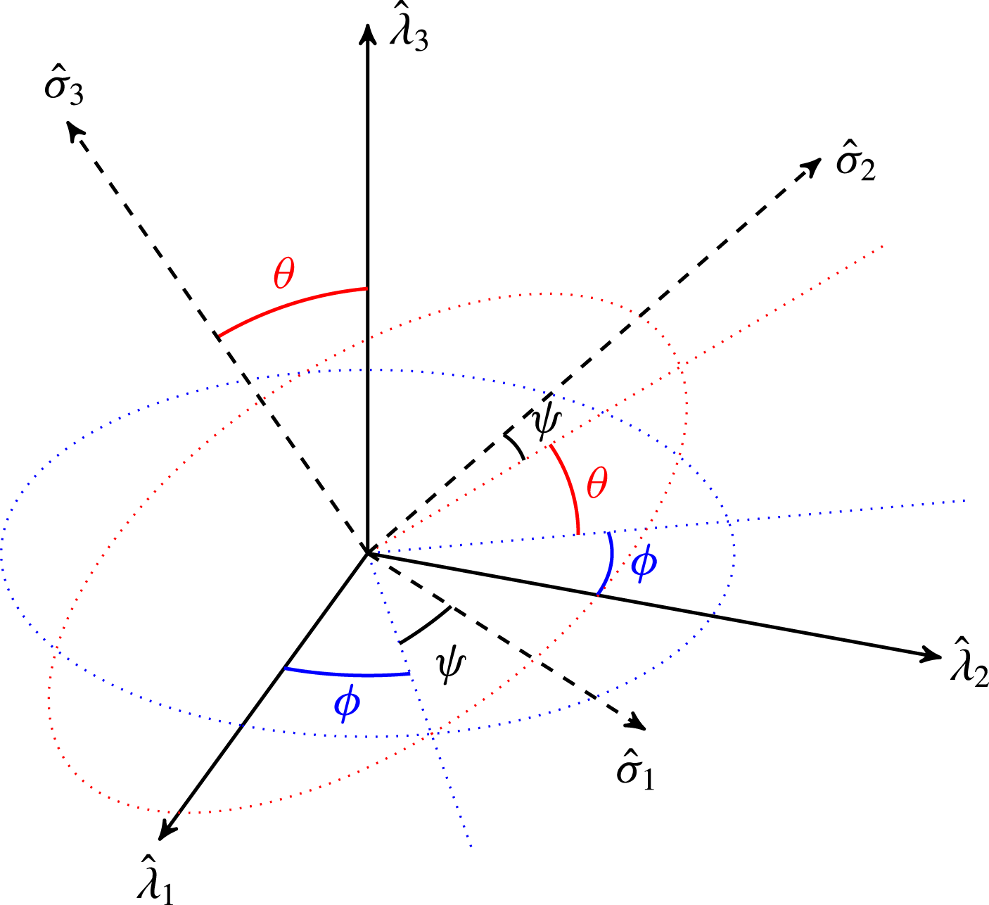
, defined as in Marion & Thornton (Reference Marion and Thornton1995) and sometimes called ZXZ Euler angles. As sketched in figure 2, to move from the eigenbasis of the stress, spanned by unit eigenvectors
 $\hat{\unicode[STIX]{x1D706}}_{\unicode[STIX]{x1D6FC}}$
, to the eigenbasis of the strain rate, spanned by unit eigenvectors
 $\hat{\unicode[STIX]{x1D70E}}_{\unicode[STIX]{x1D6FC}}$
, we first rotate by
 $\unicode[STIX]{x1D719}$
about
 $\hat{\unicode[STIX]{x1D706}}_{3}$
, then by
 $\unicode[STIX]{x1D703}$
about the rotated
 $\hat{\unicode[STIX]{x1D706}}_{1}$
and finally by
 $\unicode[STIX]{x1D713}$
about the rotated
 $\hat{\unicode[STIX]{x1D706}}_{3}$
. With this choice, the full rotation matrix
 $R(\unicode[STIX]{x1D719},\unicode[STIX]{x1D703},\unicode[STIX]{x1D713})$
that takes us from one eigenbasis to the other can be easily constructed (Marion & Thornton Reference Marion and Thornton1995).
Sketch of the orientations of the stress and strain-rate eigenframes in three-dimensions and the Euler angles that connect them. To move between the two eigenframes, we first rotate by
 $\unicode[STIX]{x1D719}$
about
 $\hat{\unicode[STIX]{x1D706}}_{3}$
, then by
 $\unicode[STIX]{x1D703}$
about the rotated
 $\hat{\unicode[STIX]{x1D706}}_{1}$
(blue dotted line), and then by
 $\unicode[STIX]{x1D713}$
about the rotated
 $\hat{\unicode[STIX]{x1D706}}_{3}$
, which is aligned with
 $\hat{\unicode[STIX]{x1D70E}}_{3}$
.

The expressions for the components of
 $R$
are somewhat lengthy; thus, we will not insert them until later, and for now will just label them as
 $R_{\unicode[STIX]{x1D6FC}\unicode[STIX]{x1D6FD}}$
. We can evaluate the matrix products and trace in (3.3) as
 $$\begin{eqnarray}\displaystyle -\tilde{\unicode[STIX]{x1D6F1}} & = & \displaystyle \text{Tr}\left[\left(\begin{array}{@{}ccc@{}}\unicode[STIX]{x1D706}_{1}R_{11} & \unicode[STIX]{x1D706}_{1}R_{21} & \unicode[STIX]{x1D706}_{1}R_{31}\\ \unicode[STIX]{x1D706}_{2}R_{12} & \unicode[STIX]{x1D706}_{2}R_{22} & \unicode[STIX]{x1D706}_{2}R_{32}\\ \unicode[STIX]{x1D706}_{3}R_{13} & \unicode[STIX]{x1D706}_{3}R_{23} & \unicode[STIX]{x1D706}_{3}R_{33}\end{array}\right)\left(\begin{array}{@{}ccc@{}}\unicode[STIX]{x1D70E}_{1}R_{11} & \unicode[STIX]{x1D70E}_{1}R_{12} & \unicode[STIX]{x1D70E}_{1}R_{13}\\ \unicode[STIX]{x1D70E}_{2}R_{21} & \unicode[STIX]{x1D70E}_{2}R_{22} & \unicode[STIX]{x1D70E}_{2}R_{23}\\ \unicode[STIX]{x1D70E}_{3}R_{31} & \unicode[STIX]{x1D70E}_{3}R_{32} & \unicode[STIX]{x1D70E}_{3}R_{33}\end{array}\right)\right]\end{eqnarray}$$
 $$\begin{eqnarray}\displaystyle & = & \displaystyle \unicode[STIX]{x1D706}_{1}\unicode[STIX]{x1D70E}_{1}R_{11}^{2}+\unicode[STIX]{x1D706}_{1}\unicode[STIX]{x1D70E}_{2}R_{21}^{2}+\unicode[STIX]{x1D706}_{1}\unicode[STIX]{x1D70E}_{3}R_{31}^{2}+\unicode[STIX]{x1D706}_{2}\unicode[STIX]{x1D70E}_{1}R_{12}^{2}+\unicode[STIX]{x1D706}_{2}\unicode[STIX]{x1D70E}_{2}R_{22}^{2}+\unicode[STIX]{x1D706}_{2}\unicode[STIX]{x1D70E}_{3}R_{32}^{2}\nonumber\\ \displaystyle & & \displaystyle +\,\unicode[STIX]{x1D706}_{3}\unicode[STIX]{x1D70E}_{1}R_{13}^{2}+\unicode[STIX]{x1D706}_{3}\unicode[STIX]{x1D70E}_{2}R_{23}^{2}+\unicode[STIX]{x1D706}_{3}\unicode[STIX]{x1D70E}_{3}R_{33}^{2}.\end{eqnarray}$$
We can use the condition that each of these tensors is deviatoric to eliminate the intermediate eigenvalues
 $\unicode[STIX]{x1D706}_{2}$
and
 $\unicode[STIX]{x1D70E}_{2}$
, which is convenient since they are sign-indeterminate. Inserting the conditions that
 $\unicode[STIX]{x1D706}_{1}+\unicode[STIX]{x1D706}_{2}+\unicode[STIX]{x1D706}_{3}=0$
and
 $\unicode[STIX]{x1D70E}_{1}+\unicode[STIX]{x1D70E}_{2}+\unicode[STIX]{x1D70E}_{3}=0$
and rearranging, we have
 $$\begin{eqnarray}\displaystyle -\tilde{\unicode[STIX]{x1D6F1}} & = & \displaystyle \unicode[STIX]{x1D706}_{1}\unicode[STIX]{x1D70E}_{1}[R_{11}^{2}-R_{21}^{2}-R_{12}^{2}+R_{22}^{2}]\nonumber\\ \displaystyle & & \displaystyle +\,\unicode[STIX]{x1D706}_{3}\unicode[STIX]{x1D70E}_{3}[R_{33}^{2}-R_{32}^{2}-R_{23}^{2}+R_{22}^{2}]\nonumber\\ \displaystyle & & \displaystyle +\,\unicode[STIX]{x1D706}_{1}\unicode[STIX]{x1D70E}_{3}[R_{31}^{2}-R_{21}^{2}-R_{32}^{2}+R_{22}^{2}]\nonumber\\ \displaystyle & & \displaystyle +\,\unicode[STIX]{x1D706}_{3}\unicode[STIX]{x1D70E}_{1}[R_{13}^{2}-R_{12}^{2}-R_{23}^{2}+R_{22}^{2}].\end{eqnarray}$$
Now we can insert the expressions for the components of
 $R$
in terms of the angles
 $\unicode[STIX]{x1D719}$
,
 $\unicode[STIX]{x1D703}$
and
 $\unicode[STIX]{x1D713}$
(Marion & Thornton Reference Marion and Thornton1995). For convenience, we introduce the shorthand notation
 $\cos \unicode[STIX]{x1D703}\equiv c_{\unicode[STIX]{x1D703}}$
and
 $\sin \unicode[STIX]{x1D703}\equiv s_{\unicode[STIX]{x1D703}}$
, and so forth. With some simplifications, we finally arrive at
 $$\begin{eqnarray}\displaystyle -\tilde{\unicode[STIX]{x1D6F1}} & = & \displaystyle \unicode[STIX]{x1D706}_{1}\unicode[STIX]{x1D70E}_{1}[(1+c_{\unicode[STIX]{x1D703}}^{2})c_{2\unicode[STIX]{x1D713}}c_{2\unicode[STIX]{x1D719}}-2c_{\unicode[STIX]{x1D703}}s_{2\unicode[STIX]{x1D719}}s_{2\unicode[STIX]{x1D713}}]\nonumber\\ \displaystyle & & \displaystyle +\,\unicode[STIX]{x1D706}_{3}\unicode[STIX]{x1D70E}_{3}[(1+c_{\unicode[STIX]{x1D703}}^{2})(1+c_{\unicode[STIX]{x1D719}}^{2})(1+c_{\unicode[STIX]{x1D713}}^{2})-3(c_{\unicode[STIX]{x1D713}}^{2}+c_{\unicode[STIX]{x1D719}}^{2})-{\textstyle \frac{1}{2}}c_{\unicode[STIX]{x1D703}}s_{2\unicode[STIX]{x1D719}}s_{2\unicode[STIX]{x1D713}}]\nonumber\\ \displaystyle & & \displaystyle +\,\unicode[STIX]{x1D706}_{1}\unicode[STIX]{x1D70E}_{3}[c_{2\unicode[STIX]{x1D719}}((1+c_{\unicode[STIX]{x1D703}}^{2})(1+c_{\unicode[STIX]{x1D713}}^{2})-3)-c_{\unicode[STIX]{x1D703}}s_{2\unicode[STIX]{x1D719}}s_{2\unicode[STIX]{x1D713}}]\nonumber\\ \displaystyle & & \displaystyle +\,\unicode[STIX]{x1D706}_{3}\unicode[STIX]{x1D70E}_{1}[c_{2\unicode[STIX]{x1D713}}((1+c_{\unicode[STIX]{x1D703}}^{2})(1+c_{\unicode[STIX]{x1D719}}^{2})-3)-c_{\unicode[STIX]{x1D703}}s_{2\unicode[STIX]{x1D719}}s_{2\unicode[STIX]{x1D713}}].\end{eqnarray}$$
Assuming that
 $\unicode[STIX]{x1D706}_{1}$
,
 $\unicode[STIX]{x1D706}_{3}$
,
 $\unicode[STIX]{x1D70E}_{1}$
and
 $\unicode[STIX]{x1D70E}_{3}$
are non-zero (which must hold if the fluid is moving and turbulent), each of the coefficients multiplying the angular terms is definite in sign. Since
 $\unicode[STIX]{x1D706}_{1},\unicode[STIX]{x1D70E}_{1}>0$
and
 $\unicode[STIX]{x1D706}_{3},\unicode[STIX]{x1D70E}_{3}<0$
, the coefficients of the first two lines in (3.7) are positive definite, while the coefficients of the last two lines are negative definite.
As a check, we can see what happens if we take the 2-D limit of (3.7). In that case, we would have
 $\unicode[STIX]{x1D706}_{1}=-\unicode[STIX]{x1D706}_{3}$
and
 $\unicode[STIX]{x1D70E}_{1}=-\unicode[STIX]{x1D70E}_{3}$
, and the angles (given our definition of Euler angles) would have to be
 $\unicode[STIX]{x1D719}=90^{\circ }$
,
 $\unicode[STIX]{x1D713}=-90^{\circ }$
, with
 $\unicode[STIX]{x1D703}=\unicode[STIX]{x1D6E9}$
remaining free. Substituting those values, we correctly recover
 $\tilde{\unicode[STIX]{x1D6F1}}=-2\unicode[STIX]{x1D706}\unicode[STIX]{x1D70E}\cos 2\unicode[STIX]{x1D6E9}$
, as above.
Let us now consider the implications of (3.7). It is immediately apparent that the expression for the flux is much more complicated in three dimensions (3.7) than in two dimensions (3.2). But the differences between three and two dimensions are more fundamental than that. First, and perhaps most significantly, unlike in the 2-D case, the flux in three dimensions cannot be factored into the product of a function only of the eigenvalues and a function only of the alignment of the eigenframes. Since we have already used the only relationship we can assert among the eigenvalues to eliminate
 $\unicode[STIX]{x1D706}_{2}$
and
 $\unicode[STIX]{x1D70E}_{2}$
, the four remaining eigenvalue products are linearly independent. Thus, the eigenvalues contribute to the flux in a fundamentally different way in three dimensions compared to two dimensions. Also unlike in two dimensions, the eigenvalues play a role in determining the sign of the flux, since the eigenvalue coefficients are of different signs in (3.7). Finally, the flux in three dimensions cannot vanish due to the geometric alignment of the eigenframes alone. Since the four eigenvalue products are linearly independent, a necessary and sufficient condition for a purely geometric suppression of the flux (that is, a way to make the flux vanish irrespective of the values of the eigenvalues) would require a simultaneous solution to the set of nonlinear equations
 $$\begin{eqnarray}\left.\begin{array}{@{}c@{}}(1+c_{\unicode[STIX]{x1D703}}^{2})c_{2\unicode[STIX]{x1D713}}c_{2\unicode[STIX]{x1D719}}-2c_{\unicode[STIX]{x1D703}}s_{2\unicode[STIX]{x1D719}}s_{2\unicode[STIX]{x1D713}}=0\\ (1+c_{\unicode[STIX]{x1D703}}^{2})(1+c_{\unicode[STIX]{x1D719}}^{2})(1+c_{\unicode[STIX]{x1D713}}^{2})-3(c_{\unicode[STIX]{x1D713}}^{2}+c_{\unicode[STIX]{x1D719}}^{2})-\frac{1}{2}c_{\unicode[STIX]{x1D703}}s_{2\unicode[STIX]{x1D719}}s_{2\unicode[STIX]{x1D713}}=0\\ c_{2\unicode[STIX]{x1D719}}((1+c_{\unicode[STIX]{x1D703}}^{2})(1+c_{\unicode[STIX]{x1D713}}^{2})-3)-c_{\unicode[STIX]{x1D703}}s_{2\unicode[STIX]{x1D719}}s_{2\unicode[STIX]{x1D713}}=0\\ c_{2\unicode[STIX]{x1D713}}((1+c_{\unicode[STIX]{x1D703}}^{2})(1+c_{\unicode[STIX]{x1D719}}^{2})-3)-c_{\unicode[STIX]{x1D703}}s_{2\unicode[STIX]{x1D719}}s_{2\unicode[STIX]{x1D713}}=0.\end{array}\right\}\end{eqnarray}$$
But this overdetermined system of four independent (nonlinear) equations in three unknowns has no solution. Thus, unlike in two dimensions, the transfer of energy between scales in three dimensions can only vanish when the eigenvalues take on specific values in conjunction with the orientation of the eigenframes. This result also means that the magnitude of the eigenvalues in three dimensions determines not only how much energy flux is possible but also how much of it actually occurs. Uncovering exactly how they are related requires appropriate normalization, since the eigenvalues of the stress and strain rate have different units. Using Kolmogorov estimates, we can define appropriate non-dimensional eigenvalues as
 $\unicode[STIX]{x1D706}_{\unicode[STIX]{x1D6FC}}^{\ast }=\unicode[STIX]{x1D706}_{\unicode[STIX]{x1D6FC}}(\unicode[STIX]{x1D716}r)^{-2/3}$
and
 $\unicode[STIX]{x1D70E}_{\unicode[STIX]{x1D6FC}}^{\ast }=\unicode[STIX]{x1D70E}_{\unicode[STIX]{x1D6FC}}(r^{2}/\unicode[STIX]{x1D716})^{1/3}$
, where
 $\unicode[STIX]{x1D716}$
is the energy dissipation rate and
 $r$
is the length scale in the cascade we are considering. Note that this choice gives
 $\unicode[STIX]{x1D706}_{\unicode[STIX]{x1D6FC}}^{\ast }\unicode[STIX]{x1D70E}_{\unicode[STIX]{x1D6FC}}^{\ast }=\unicode[STIX]{x1D706}_{\unicode[STIX]{x1D6FC}}\unicode[STIX]{x1D70E}_{\unicode[STIX]{x1D6FC}}/\unicode[STIX]{x1D716}$
, as one would expect.
4 Efficiency of energy transfer in the cascade
Now that we have worked out the general nature of the inner product between
 $\tilde{\unicode[STIX]{x1D70F}}_{ij}$
and
 $\tilde{\unicode[STIX]{x1D634}}_{ij}$
, we can begin to relate it back to turbulence and the role played by these tensors and their alignment in the cascade. As discussed in § 2, when
 $\tilde{\unicode[STIX]{x1D70F}}_{ij}$
and
 $\tilde{\unicode[STIX]{x1D634}}_{ij}$
are aligned, mechanical work is done by some scales on the others, and energy is transferred between them. When they are perfectly misaligned, however, no work is done even though the stress and strain rate themselves may be large in magnitude. This situation does not imply that the stress has no effects; rather, in the misaligned case it is purely responsible for driving transport in the resolved field, with no coupling to other scales.
In two dimensions, it is straightforward to connect the tensor alignment to the energy flux. Equation (3.2) tells us that the energy flux between scales is given by
 $-2\unicode[STIX]{x1D706}\unicode[STIX]{x1D70E}\cos 2\unicode[STIX]{x1D6E9}$
. Given a pair of eigenvalues
 $\unicode[STIX]{x1D706}$
and
 $\unicode[STIX]{x1D70E}$
, this expression is at its largest (in magnitude) when
 $\unicode[STIX]{x1D6E9}=0$
or
 $\unicode[STIX]{x03C0}/2$
, but vanishes when
 $\unicode[STIX]{x1D6E9}=\unicode[STIX]{x03C0}/4$
. Thus, the angular part
 $\cos 2\unicode[STIX]{x1D6E9}$
, which is bounded between
 $0$
and
 $1$
, directly tells us the fraction of the available turbulent stress that does work against the strain rate to transfer energy between scales. Because of this property, we recently suggested that this angular part can be thought of as an ‘efficiency’ for the energy cascade (Fang & Ouellette Reference Fang and Ouellette2016), and showed that this efficiency is fairly low (approximately 27 %, on average) in 2-D turbulence.
We can now generalize this idea to the 3-D case. In general, the energy flux is a function of the stress and strain-rate eigenvalues and the three Euler angles that link their eigenframes; that is,
 $\tilde{\unicode[STIX]{x1D6F1}}=\tilde{\unicode[STIX]{x1D6F1}}(\unicode[STIX]{x1D706}_{\unicode[STIX]{x1D6FC}},\unicode[STIX]{x1D70E}_{\unicode[STIX]{x1D6FC}},\unicode[STIX]{x1D719},\unicode[STIX]{x1D703},\unicode[STIX]{x1D713})$
. We then define the cascade efficiency to be
 $$\begin{eqnarray}\unicode[STIX]{x1D6E4}=\frac{\tilde{\unicode[STIX]{x1D6F1}}(\unicode[STIX]{x1D706}_{\unicode[STIX]{x1D6FC}},\unicode[STIX]{x1D70E}_{\unicode[STIX]{x1D6FC}},\unicode[STIX]{x1D719},\unicode[STIX]{x1D703},\unicode[STIX]{x1D713})}{\tilde{\unicode[STIX]{x1D6F1}}_{max}(\unicode[STIX]{x1D706}_{\unicode[STIX]{x1D6FC}},\unicode[STIX]{x1D70E}_{\unicode[STIX]{x1D6FC}})}.\end{eqnarray}$$
We define
 $\tilde{\unicode[STIX]{x1D6F1}}_{max}(\unicode[STIX]{x1D706}_{\unicode[STIX]{x1D6FC}},\unicode[STIX]{x1D70E}_{\unicode[STIX]{x1D6FC}})$
as
 $\max _{\unicode[STIX]{x1D719},\unicode[STIX]{x1D703},\unicode[STIX]{x1D713}}[\text{sign}(\tilde{\unicode[STIX]{x1D6F1}})\tilde{\unicode[STIX]{x1D6F1}}(\unicode[STIX]{x1D706}_{\unicode[STIX]{x1D6FC}},\unicode[STIX]{x1D70E}_{\unicode[STIX]{x1D6FC}},\unicode[STIX]{x1D719},\unicode[STIX]{x1D703},\unicode[STIX]{x1D713})]$
. That is,
 $\unicode[STIX]{x1D6E4}$
is the ratio of the energy flux between scales that actually occurs at a given spatio-temporal location to the maximum that would be possible if the eigenframes of the stress and the strain rate were optimally aligned (regardless of whether this maximum value actually corresponds to a solution of the Navier–Stokes equations). We include the
 $\text{sign}(\tilde{\unicode[STIX]{x1D6F1}})$
term to maintain the character of the energy flux (that is, backscatter or forward scatter), and note that the maximum positive and maximum negative fluxes are typically very similar. The analogous expression for the 2-D case is given by
 $-\!\cos 2\unicode[STIX]{x1D6E9}$
, as expected from our discussion above. In three dimensions, however, because the angular parts of (3.7) cannot be factored out of the expression for
 $\tilde{\unicode[STIX]{x1D6F1}}$
, the situation is much more complicated and
 $\unicode[STIX]{x1D6E4}$
cannot be written in a compact form. But as we show in § 5,
 $\unicode[STIX]{x1D6E4}$
can be calculated at every spatial point, so that we can at least make empirical statements about how much of the available energy at each scale in the cascade is actually transferred to other scales.
5 Direct numerical simulation results
5.1 Data set
To make the above discussion of geometry in the cascade more concrete, we measured scale-to-scale fluxes and the cascade efficiency in a direct numerical simulation (DNS) of forced isotropic turbulence. Data were obtained from the Johns Hopkins Turbulence Database (JHTDB). Complete details of the simulation can be found on the JHTDB website and in Li et al. (Reference Li, Perlman, Wan, Yang, Meneveau, Burns, Chen, Szalay and Eyink2008). Briefly, to generate the data the Navier–Stokes equations were solved via a pseudo-spectral algorithm in a triply periodic box of dimensions
 $2\unicode[STIX]{x03C0}\times 2\unicode[STIX]{x03C0}\times 2\unicode[STIX]{x03C0}$
on a grid of
 $1024^{3}$
points. The Taylor microscale Reynolds number of the flow was
 $R_{\unicode[STIX]{x1D706}}=433$
.
Data are stored in the database for approximately five eddy turnover times on a relatively small time step. For our analysis, however, we require only Eulerian snapshots. For our less computationally expensive calculations, we used 1024 such snapshots. For quantities that were more time consuming to calculate, we used fewer, but all the calculations reported below were averaged over at least 36 independent velocity fields.
5.2 Filtering analysis
In our discussion so far, we have not specified the precise form of the projection operation
 ${\mathcal{P}}$
that removes degrees of freedom from the velocity field. To study the geometry of the cascade from an actual data set, however, we need to do so. We choose here to take a filtering approach, which allows us to resolve spectral processes in space and time (Germano Reference Germano1992; Liu, Meneveau & Katz Reference Liu, Meneveau and Katz1994; Eyink Reference Eyink1995; Chen et al.
Reference Chen, Ecke, Eyink, Wang and Xiao2003, Reference Chen, Ecke, Eyink, Rivera, Wan and Xiao2006; Rivera et al.
Reference Rivera, Daniel, Chen and Ecke2003; Liao & Ouellette Reference Liao and Ouellette2013, Reference Liao and Ouellette2014).
Briefly, since we have discussed the filtering approach in detail before (Liao & Ouellette Reference Liao and Ouellette2013, Reference Liao and Ouellette2014), we remove the small scales from the velocity field
 $u_{i}(\boldsymbol{x})$
by convolving it with a function that suppresses high wavenumbers in Fourier space, so that
 $$\begin{eqnarray}\tilde{u} _{i}(\boldsymbol{x})=\int G_{r}(\boldsymbol{x}-\boldsymbol{x}^{\prime })u_{i}(\boldsymbol{x}^{\prime })\,\text{d}\boldsymbol{x}^{\prime }.\end{eqnarray}$$
Here,
 $G_{r}$
is the filter kernel; the subscript
 $r$
denotes the smallest remaining length scale after filtering. Our results are not very sensitive to the precise form of
 $G_{r}$
; we here use a sharp spectral filter (with a cutoff at
 $r$
) smoothed with a sine function to avoid ringing. All of the discussion above in § 2 holds when the projection operation
 ${\mathcal{P}}$
is this filtering. We also note that although this process is similar in spirit to a large-eddy simulation approach, it does not neglect backscatter, as a classic Smagorinsky model would. Rather, since we filter only after computing the full velocity field, small-scale processes that affect the large scales are still present even after filtering.
5.3 Flux and efficiency
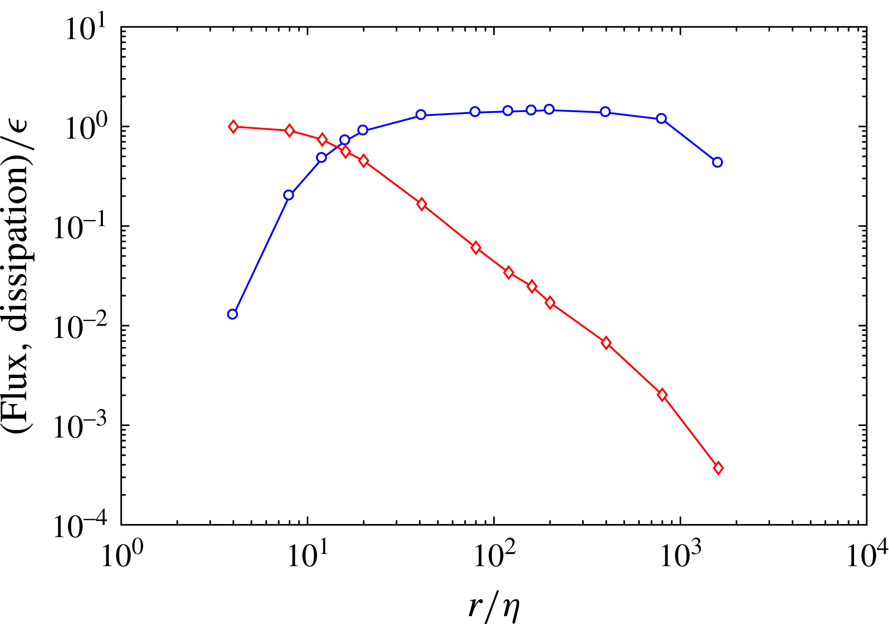
Mean scale-to-scale energy flux
 $\langle \tilde{\unicode[STIX]{x1D6F1}}\rangle$
(circles) and the mean viscous dissipation
 $2\unicode[STIX]{x1D708}\langle \tilde{\unicode[STIX]{x1D634}}_{ij}\tilde{\unicode[STIX]{x1D634}}_{ij}\rangle$
(diamonds) as a function of
 $r/\unicode[STIX]{x1D702}$
. Both the flux and the dissipation are scaled by
 $\unicode[STIX]{x1D716}$
.

As a first benchmark of our methods, we computed the mean energy flux
 $\langle \tilde{\unicode[STIX]{x1D6F1}}\rangle$
as a function of scale
 $r$
, where the average is taken over space, as shown in figure 3. As expected, the flux is nearly constant with
 $r$
and approximately equal to the dissipation rate
 $\unicode[STIX]{x1D716}$
in the inertial range (over a range of approximately
 $50\unicode[STIX]{x1D702}<r<1000\unicode[STIX]{x1D702}$
, where
 $\unicode[STIX]{x1D702}$
is the Kolmogorov scale), but falls off in the dissipation range where the energy transfer between scales is expected to be weak. The mean scale-dependent viscous dissipation
 $2\unicode[STIX]{x1D708}\langle \tilde{\unicode[STIX]{x1D634}}_{ij}\tilde{\unicode[STIX]{x1D634}}_{ij}\rangle$
, also shown in figure 3, is weak in the inertial range but dominant (and approximately equal to
 $\unicode[STIX]{x1D716}$
) in the dissipation range. Thus, our filtered results are consistent with what one would expect in turbulent flow, and which one could measure via other means.
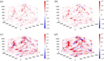
(a,b) Slices through the
 $\tilde{\unicode[STIX]{x1D6F1}}$
field at a single time for (a)
 $r=120\unicode[STIX]{x1D702}$
and (b)
 $r=200\unicode[STIX]{x1D702}$
. The colour scale gives the value of
 $\tilde{\unicode[STIX]{x1D6F1}}$
in computational units; for comparison, the mean value of the dissipation rate
 $\unicode[STIX]{x1D716}$
is approximately 0.05. (c,d)
 $\max \tilde{\unicode[STIX]{x1D6F1}}$
(that is, the denominator of (4.1)) for the same data and filter scales, shown with the same colour scale.

More interesting is the spatial distribution of
 $\tilde{\unicode[STIX]{x1D6F1}}$
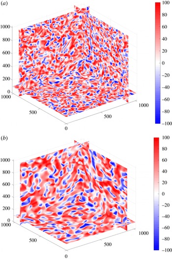
at different scales, which is only available through some kind of filtering approach. In figure 4(a,b), we show slices through the
 $\tilde{\unicode[STIX]{x1D6F1}}$
field for a single snapshot in time at two scales in the inertial range,
 $r=120\unicode[STIX]{x1D702}$
and
 $r=200\unicode[STIX]{x1D702}$
. In both cases,
 $\tilde{\unicode[STIX]{x1D6F1}}$
is highly spatially variable, and shows both positive and negative values, even though the spatial average is weakly positive. But even though
 $\tilde{\unicode[STIX]{x1D6F1}}$
is quite intermittent, its extreme values are much less intense than they could be if
 $\tilde{\unicode[STIX]{x1D70F}}_{ij}$
and
 $\tilde{\unicode[STIX]{x1D634}}_{ij}$
were perfectly aligned. In figure 4(c,d), we show the same slices and snapshots as in figure 4(a,b) for
 $\tilde{\unicode[STIX]{x1D6F1}}_{max}$
(the denominator of (4.1)); that is, the largest the energy flux could possibly be in each location given the magnitudes of the stress and strain rate. To find this value, we simply searched through the space of possible values of
 $\unicode[STIX]{x1D719}$
,
 $\unicode[STIX]{x1D703}$
and
 $\unicode[STIX]{x1D713}$
until
 $\tilde{\unicode[STIX]{x1D6F1}}$
was maximized.
The efficiency
 $\unicode[STIX]{x1D6E4}$
(as a percentage) for the same data and filter scales as in figure 4. Negative values of
 $\unicode[STIX]{x1D6E4}$
show those places where the energy flux is directed toward larger scales.

With both the numerator and denominator of (4.1) measured, we can compute the efficiency
 $\unicode[STIX]{x1D6E4}$
. In figure 5, we show
 $\unicode[STIX]{x1D6E4}$
computed for the same data shown in figure 4. It is clear that
 $\unicode[STIX]{x1D6E4}$
is highly spatially variable, and is not high only in places where the flux itself is high; that is, the turbulence can be efficient at transferring energy even if there not a significant amount of energy to transfer. Negative values of
 $\unicode[STIX]{x1D6E4}$
mark places in the flow where the energy flux is directed to larger scales rather than the typical forward transfer to smaller scales.
The average efficiency
 $\langle \unicode[STIX]{x1D6E4}\rangle$
(expressed as a percentage) as a function of
 $r/\unicode[STIX]{x1D702}$
. The mean efficiency saturates in the inertial range at approximately 25 %, and decreases rapidly in the dissipation range.

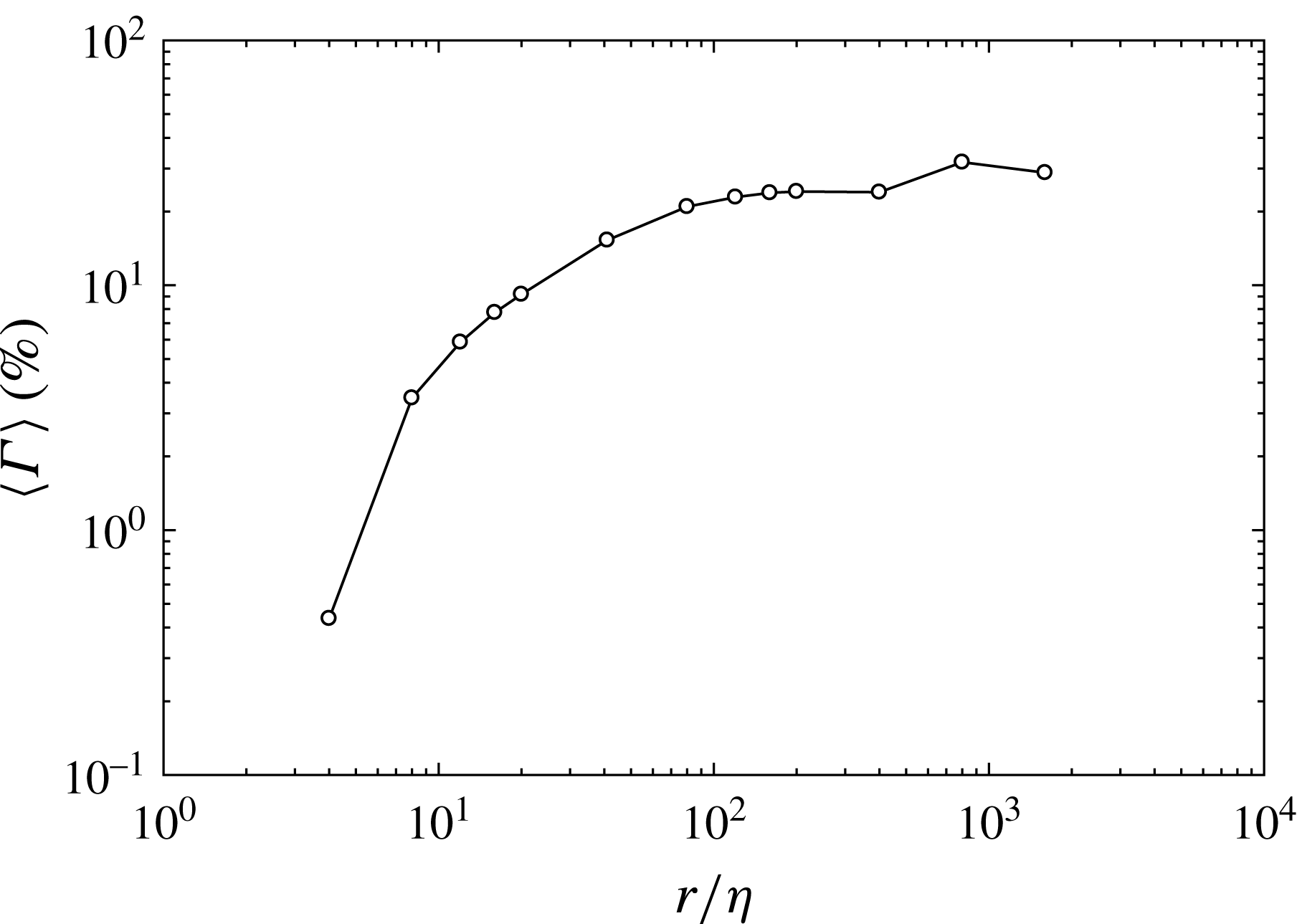
Looking at fields is informative, but it is also useful to compute the average efficiency to understand what the ‘typical’ turbulence behaviour is. In figure 6, we show the average efficiency
 $\langle \unicode[STIX]{x1D6E4}\rangle$
as a function of scale. Two aspects of this curve are particularly noteworthy. First,
 $\langle \unicode[STIX]{x1D6E4}\rangle$
saturates in the inertial range at a perhaps surprisingly low value of approximately 25 %. As a point of comparison, if we assume that the stress and strain rate are related by a Boussinesq eddy-viscosity closure or a Smagorinsky model, both of which take the eigenframes of the stress and strain rate to be aligned (Pope Reference Pope2000), and compute
 $\langle \unicode[STIX]{x1D6E4}\rangle$
in the same way as we have done here for the DNS data, we find a value of 96 % – much higher than what we find for the DNS. This value of 25 % is also comparable with what we previously found in 2-D turbulence (Fang & Ouellette Reference Fang and Ouellette2016). It indicates that on the average approximately three quarters of the available scale-dependent stress is used to move energy around in space rather than to pump it to different scales. We also find that
 $\langle \unicode[STIX]{x1D6E4}\rangle$
decreases very rapidly as
 $r\rightarrow \unicode[STIX]{x1D702}$
; thus, not only is there not much energy to transfer between scales in the dissipation range, since so much of it has been removed by viscous forces, but the turbulence is also very inefficient at transferring what energy remains between scales. This result is not a priori obvious; although it is expected that the energy flux is weak in the dissipation range, that does not mean that the transfer also needs to be inefficient.
5.4 Alignment
To try to gain additional insight as to why the efficiency drops so rapidly in the dissipation range as well as what is driving the efficiency to be low throughout the cascade, we also computed statistics of the eigenvalues and eigenframe alignments that go into the scale-to-scale energy flux (3.7). We looked at three different filter scales:
 $r=8\unicode[STIX]{x1D702}$
in the dissipation range,
 $r=51\unicode[STIX]{x1D702}$
at the bottom of the inertial range, and
 $r=400\unicode[STIX]{x1D702}$
well into the inertial range.
Probability density functions (p.d.f.s) of the product of the positive eigenvalues of the stress and strain rate normalized by
 $\unicode[STIX]{x1D716}$
for three filter scales:
 $r=8\unicode[STIX]{x1D702}$
(solid black line),
 $r=51\unicode[STIX]{x1D702}$
(blue dashed line) and
 $r=400\unicode[STIX]{x1D702}$
(red dash-dotted line).

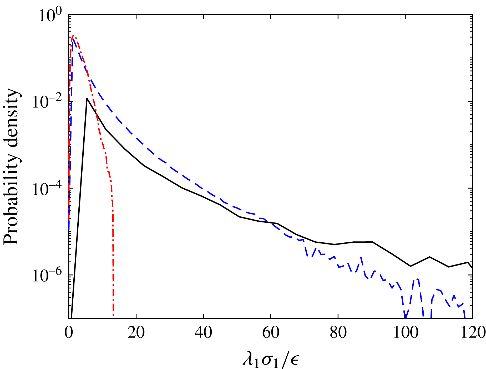
In figure 7, we plot the probability density functions (p.d.f.s) of the product of the positive stress and strain-rate eigenvalues (that is,
 $\unicode[STIX]{x1D706}_{1}\unicode[STIX]{x1D70E}_{1}$
) at these three scales. The shape of the p.d.f.s of the other three eigenvalue combinations in (3.7) is similar. For
 $r=8\unicode[STIX]{x1D702}$
, the p.d.f. is very broad, meaning that the eigenvalues fluctuate wildly, suggesting that the magnitudes of the stress and strain rate are very dynamic at these scales. Similar behaviour is seen for
 $r=51\unicode[STIX]{x1D702}$
at the transition between the dissipation and inertial ranges. But by
 $r=400\unicode[STIX]{x1D702}$
, the p.d.f. of
 $\unicode[STIX]{x1D706}_{1}\unicode[STIX]{x1D70E}_{1}$
is much narrower, suggesting the magnitudes of the stress and strain rate fluctuate less. This reduction in the degree of fluctuation of the eigenvalues may in turn be partially responsible for the more efficient scale-to-scale energy transfer: because the efficiency depends on the eigenvalues as well as the eigenframe alignment in three dimensions (in that the optimal alignment may depend on the eigenvalues) and the eigenframe alignment takes time to change (Xu, Pumir & Bodenschatz Reference Xu, Pumir and Bodenschatz2011; Ni, Ouellette & Voth Reference Ni, Ouellette and Voth2014; Fang & Ouellette Reference Fang and Ouellette2016), more coherent eigenvalues may allow the eigenframes to adjust to more optimal, efficient alignments before the flow changes. The magnitudes of the eigenvalues themselves then get scaled out of the efficiency calculation, as defined in (4.1).
Joint p.d.f.s of the Euler angles relating the stress and strain-rate eigenframes for (a,b,c)
 $r=8\unicode[STIX]{x1D702}$
, (d,e,f)
 $r=51\unicode[STIX]{x1D702}$
and (g,h,i)
 $r=400\unicode[STIX]{x1D702}$
.

Because the alignment of the eigenframes is the more important driver of the efficiency, we also computed the statistics of the Euler angles
 $\unicode[STIX]{x1D719}$
,
 $\unicode[STIX]{x1D703}$
and
 $\unicode[STIX]{x1D713}$
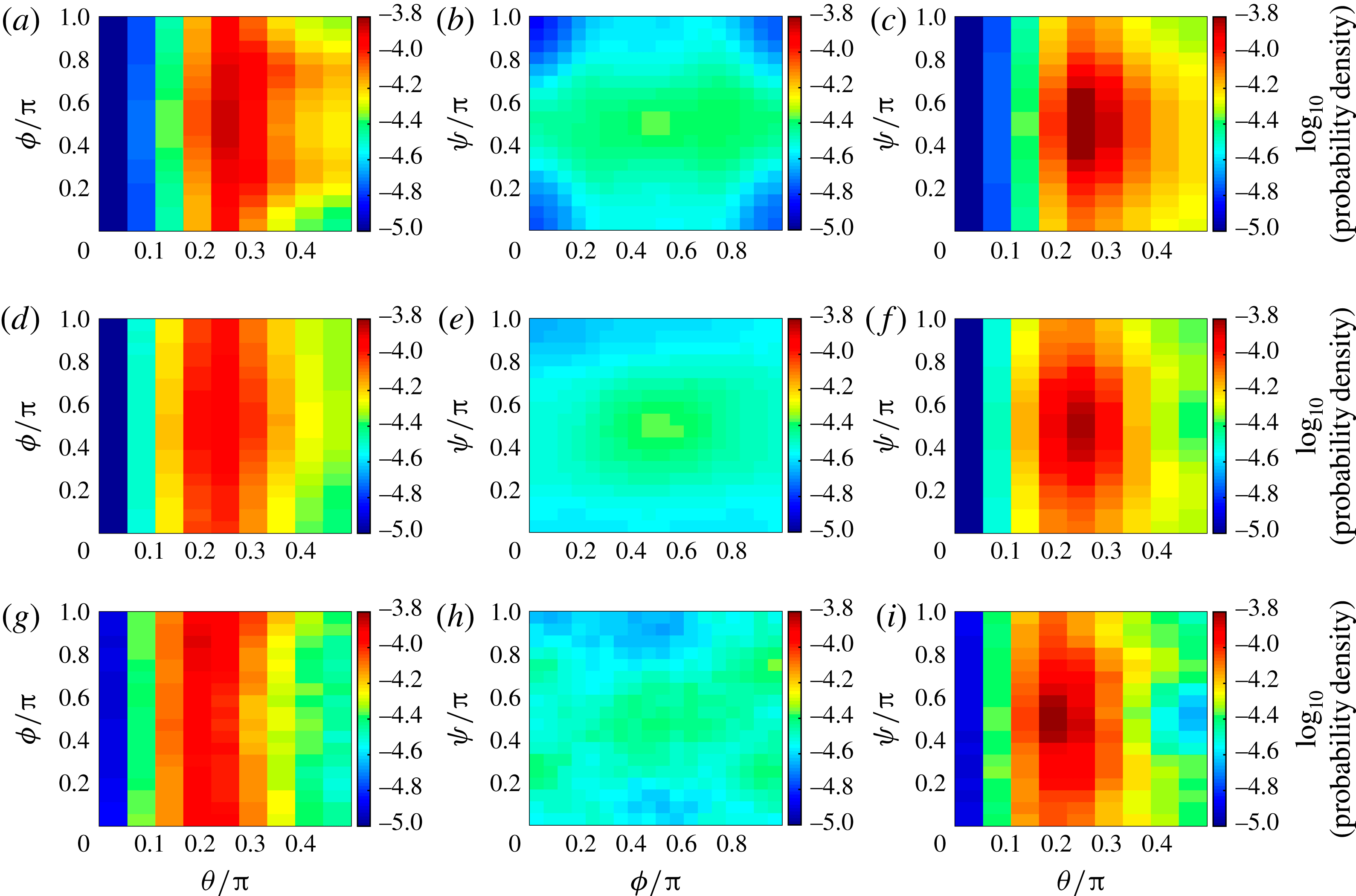
that relate the two eigenframes at the same three filter scales. In figure 8, we show the three independent joint p.d.f.s of these angles for each of the three scales we are considering. First, let us note that the efficiency of the energy transfer tends to be very high when the eigenframes of the stress and strain rate are aligned or anti-aligned (as discussed above for Boussinesq or Smagorinsky closures); that is, for
 $\unicode[STIX]{x1D719}$
approximately
 $0$
,
 $\unicode[STIX]{x03C0}/2$
or
 $\unicode[STIX]{x03C0}$
,
 $\unicode[STIX]{x1D703}$
approximately
 $0$
or
 $\unicode[STIX]{x03C0}/2$
(since
 $\unicode[STIX]{x1D703}$
has a restricted range) and
 $\unicode[STIX]{x1D713}$
approximately
 $0$
,
 $\unicode[STIX]{x03C0}/2$
or
 $\unicode[STIX]{x03C0}$
. Thus, the most efficient energy transfer would occur for values of the angles in the corners of the joint p.d.f.s in figure 8, and additionally in the centre of the joint p.d.f.s of
 $\unicode[STIX]{x1D719}$
and
 $\unicode[STIX]{x1D713}$
in the central column.
This is not, however, what we observe. In the dissipation range (
 $r=8\unicode[STIX]{x1D702}$
), the joint p.d.f.s are all fairly significantly peaked, but these peaks tend to lie near the centres of the ranges for each angle, where the eigenframes are close to optimally misaligned. There is very little statistical weight near the corners of the ranges, where the transfer is efficient. As we increase the filter scale to
 $r=51\unicode[STIX]{x1D702}$
, the joint p.d.f.s flatten somewhat, and more weight appears near the optimal angles; and, correspondingly, the efficiency goes up (see figure 5). By
 $r=400\unicode[STIX]{x1D702}$
, the joint p.d.f.s have flattened yet more, while also developing secondary peaks near the optimal angles. Thus, the increase in efficiency appears to be partially due to the development of these secondary peaks in the angle statistics and partially due to the overall flattening of the joint p.d.f.s, so that alignments that are closer to optimal are seen much more frequently because the overall statistics of the alignment are more random. These effects are particularly apparent in the statistics of
 $\unicode[STIX]{x1D719}$
and
 $\unicode[STIX]{x1D713}$
, while
 $\unicode[STIX]{x1D703}$
changes less with scale. In particular, looking at figure 8(b,e,h), we see that the joint p.d.f. of
 $\unicode[STIX]{x1D719}$
and
 $\unicode[STIX]{x1D713}$
has little weight near the optimal angles (located at the corners and centre of the plot) for
 $r=8\unicode[STIX]{x1D702}$
, leading to the poor efficiency at this scale. By
 $r=51\unicode[STIX]{x1D702}$
, the two suboptimal peaks in the joint p.d.f. have merged into one peak in the middle of the plot, where the alignment is more favourable – and correspondingly the efficiency is higher. And by
 $r=400\unicode[STIX]{x1D702}$
, peaks have also begun to develop in the corners of the plot, leading to yet higher efficiency. These systematic effects suggest the presence of some physical mechanism driving eigenframe alignments; but what this mechanism is remains mysterious.
6 Discussion and conclusions
The primary goal of our work here has been to recast the turbulent energy cascade in purely mechanical terms, so that the spectral energy flux between scales is described as the effect of some scales doing mechanical work on others. Describing the cascade in this way naturally brings geometry into the problem, since no work can be done, and therefore no energy transferred, if the stress and strain rate are misaligned. We showed that the geometric alignment of these two tensors is quite different in two and three dimensions. In particular, the inner product between the stress and the strain rate factors into a product of a part related only to the tensor magnitudes and a part related only to the alignment of their eigenframes in two dimensions, while in three dimensions the magnitude and frame alignment are inextricably mixed.
This result has many implications, some of which we have explored here and others that we leave for future work. Thinking about how the relative alignment of the stress and strain-rate eigenframes impacts the amount of energy that can be transferred between scales, we defined an efficiency for the cascade process. We measured this efficiency from a 3-D DNS, and found that on average it is lower than one might naively expect (and comparable with our previous results in 2-D turbulence experiments (Fang & Ouellette Reference Fang and Ouellette2016)). This observation suggests that most of the available turbulent stress drives spatial transport rather than the net energy cascade. An intriguing way to study this connection between the turbulent stress and spatial transport might be to decompose the resolved strain rate or stress fields into local and non-local contributions, in the spirit of Hamlington, Schumacher & Dahm (Reference Hamlington, Schumacher and Dahm2008a ,Reference Hamlington, Schumacher and Dahm b ). There is also much more work to be done to understand exactly what determines the turbulent efficiency, particularly at the pointwise level. It is even conceivable that this kind of study may be able to contribute to Reynolds-averaged Navier–Stokes (RANS) or large-eddy simulation (LES) modelling, both of which explicitly seek to write the turbulent stress in terms of other available flow quantities. For that reason, it would be interesting to explore any potential Reynolds number dependence of our results, which we have not done here since the JHTDB contains a data set at only one Reynolds number.
Our work also points to an important way in which 2-D and 3-D turbulence are different from a purely geometric perspective: the difference in dimensionality means that the tensor eigenvalues influence the stress/strain-rate inner product in fundamentally different ways. Thus, variations in the eigenvalues may affect the energy flux in more complicated ways in three than in two dimensions, since they couple to the eigenframe alignment differently. In particular, spatial gradients in the eigenvalues and eigenframe relative angles may lead to steeper gradients in the scale-to-scale energy flux in 3-D turbulence. Suggestively, steep gradients in dissipation (or flux) are usually thought to be an important ingredient in intermittency; and, the 2-D inverse cascade is thought to be non-intermittent, while the 3-D forward cascade certainly is. Yet, at the same time we find that the efficiencies in two and three dimensions are quite similar. Much more work therefore needs to be done to understand these observations, but we expect this to be a productive direction for future research.
Acknowledgements
We thank S. Ameli and S. Shadden for helpful discussions on the differences between the stress/strain-rate inner product in 2-D and 3-D flow. This work was partially supported by the US National Science Foundation under grant no. CBET-1600292.