2.1. The governing equation

We consider the displacement process of two viscous fluids upon the injection of one of them into a horizontal and homogeneous porous layer with permeability $k$ , porosity $\phi$ and finite depth $h_0$ , as shown in figure 1. In particular, fluid 1 is being injected to displace ambient fluid 2 at a constant area rate $q$ , which initially fills up the pore space of the porous layer. The density and viscosity of the fluids are denoted by $\rho _1,\rho _2,\mu _1$ and $\mu _2$ , respectively. Assuming that fluids 1 and 2 are immiscible, the interface shape between them is denoted by $h(x,t)$ , and the pressure distribution is denoted by $p(x,y,t)$ . We also neglect the influence of wetting and interfacial tension within the length and time scales of the model problem. This is the classic model set-up of a series of previous studies with the focus on the interface shape evolution (e.g. Huppert & Woods Reference Huppert and Woods1995; Pegler et al. Reference Pegler, Huppert and Neufeld2014; Zheng et al. Reference Zheng, Guo, Christov, Celia and Stone2015b ), and our discussion on pressure evolution in the present work is based on these previous efforts.

When the length of the current is much greater than its thickness, the theory of lubricating flow indicates that the vertical velocity $v$ of the current is much smaller than the horizontal velocity $u$ , and hence the flow in the porous layer is one-dimensional at leading order. In this case, the pressure takes the hydrostatic distribution within the domain. If we denote the background pressure along the base $(y=0)$ of the horizontal porous layer as $p_0(x,t)$ , hydrostatic pressure distribution then indicates that pressure $p(x,y,t)$ is given by

(2.1) \begin{equation} p(x,y,t) = \begin{cases} p_0(x,t)-\rho _1 gy, &0\leqslant x \lt x_s(t),\ 0 \leqslant y \lt h_0,\\ p_0(x,t)-\rho _1 gy, &x_s(t)\leqslant x \lt x_{\!f}(t),\ 0\leqslant y \lt h,\\ p_0(x,t)-\rho _1 gh-\rho _2 g(y-h), &x_s(t)\leqslant x \lt x_{\!f}(t), \ h\leqslant y \leqslant h_0,\\ p_0(x,t)-\rho _2 gy, &x \geqslant x_{\!f}(t),\ 0\leqslant y \leqslant h_0, \end{cases} \end{equation}

where $x_{\!f}(t)$ and $x_s(t)$ denote the leading and (possibly) trailing fronts of the fluid–fluid interface $h(x,t)$ , respectively, as defined by $h(x_{\!f}(t),t)=0$ and $h(x_s(t),t)=h_0$ .

Previous studies indicate that the background pressure gradient $\partial p_0/\partial x$ is under the influence of both fluid injection and buoyancy, as given by

(2.2) \begin{equation} \frac {\partial p_0}{\partial x} = -\frac {\mu _1 \mu _2 q}{\mu _2 kh + \mu _1 k(h_0-h)} + \frac {\mu _1 \Delta \rho gk (h_0-h)}{\mu _2 kh + \mu _1 k(h_0-h)} \frac {\partial h}{\partial x}, \end{equation}

where $\Delta \rho \equiv \rho _1-\rho _2\gt 0$ . The first term on the right-hand side of (2.2) represents the influence of fluid injection and is proportional to the injection rate $q$ , while the second term on the right-hand side of (2.2) represents the influence of buoyancy-driven flow and is proportional to the density difference $\Delta \rho$ and the local slope of the fluid–fluid interface $\partial h/\partial x$ . Upon integration of solution (2.2) in $x$ , we arrive at an expression for the evolution of the background pressure $p_0(x,t)$ at any downstream location $x$ of interest:

(2.3) \begin{equation} p_0(x,t) = p_0(0,t) -\int _0^x \left [\frac {\mu _1 \mu _2 q}{\mu _2 kh + \mu _1 k(h_0-h)} - \frac {\mu _1 \Delta \rho gk (h_0-h)}{\mu _2 kh + \mu _1 k(h_0-h)} \frac {\partial h}{\partial \hat {x}}\right ] \mathrm{d} \hat {x}, \end{equation}

where $p_0(0,t)$ denotes pressure evolution at the source $(x=0)$ , the location of the well bore. The value of $p_0(0,t)$ is typically related to the weight of the fluid in the pore space between its location and the ground surface, and hence $p_0(0,t)$ could be time independent at leading order. In fact, it is more convenient to discuss the background pressure drop measured from its source value, defined as $\Delta p_0(x,t) \equiv p_0(0,t)-p_0(x,t)$ , which we employ later in the present work. In particular, it is seen that solution (2.3) for $p_0(x,t)$ depends explicitly on the profile shape evolution $h(x,t)$ , which has been studied before and we review briefly in Appendix A for completeness of the description.

2.2. Non-dimensionlisation

It is standard to study the model problem in the dimensionless space. Choosing $t_c \equiv \Delta \rho gk \phi h_0^3 / (\mu _1 q^2)$ and $x_c \equiv \Delta \rho gkh_0^2 / (\mu _1 q)$ as the characteristic time and length scales, respectively, we define dimensionless time $T \equiv t/t_c$ , length $X \equiv x/x_c$ and thickness $H \equiv h/h_0$ . Physically, $t_c$ and $x_c$ arise due to the competition between buoyancy and injection forces, and $h_0$ is simply the thickness of the porous layer. The scales are chosen such that at $t = t_c$ the front locates at $x_{\!f} \approx x_c$ for moderate values of $M$ , and with this specific set of scales, the prefactors of the dimensionless partial differential equations (PDEs) and initial and boundary conditions (IBCs) become one (see also Appendix A).

Notice again that the focus of the present work is on pressure. If we choose $p_c \equiv \Delta \rho gh_0$ , a hydrostatic pressure head, as the characteristic pressure, the dimensionless background pressure drop $\Delta P_0(X,T)$ along the base of the porous layer can be obtained as

(2.4) \begin{align} \Delta P_0(X,T)\equiv P_0(0,T)-P_0(X,T) = \int _0^X \left [\frac {M}{1 + (M-1) H} - \frac {1-H}{1 + (M-1) H} \frac {\partial H}{\partial \hat {X}} \right ]\mathrm{d}\hat {X}. \end{align}

Since fluids always move in the direction of pressure decrease for pressure-driven flows, the definition $\Delta P_0(X,T) \equiv P_0(0,T)-P(X,T)$ ensures that $\Delta P_0(X,T)$ is non-negative. We can also define dimensionless pressure drop $\Delta P(X,Y,T) \equiv P_0(0,T)-P(X,Y,T) \geqslant 0$ and obtain

(2.5) \begin{equation} \Delta P(X,Y,T) \equiv P_0(0,T)-P(X,Y,T) = \Delta P_0(X,T)+\frac {Y}{G}+(H-Y)\mathcal{H}(Y-H), \end{equation}

for $X\geqslant 0$ and $0\leqslant Y\leqslant 1$ , where the Heaviside step function in solution (2.5) is defined as

(2.6) \begin{equation} \mathcal{H}(z) =\left \{ \begin{aligned} &0,&z\lt 0,\\ &1,&z\geqslant 0. \end{aligned} \right . \end{equation}

A second dimensionless parameter $G \equiv \Delta \rho /\rho _1$ is recognised in (2.5) for the distribution of pressure, which measures the relative strength of buoyancy compared with the density of the injecting fluid 1. The definition and physical meaning of the dimensionless parameters $M$ and $G$ are summarised also in table 1.

Table 1.

Definition and physical meaning of the two dimensionless parameters $M$ and $G$ that impact the pressure distribution within a porous layer of finite depth during fluid injections.

Figure 2.

Early-time self-similar behaviour of the background pressure drop $\Delta P_0(X,T)$ at different times and at different monitoring locations when $T \ll 1$ , with $M=2$ as an example: (a) numerical solutions of (2.4) at $T=\{0.2,0.4,0.6,0.8,1\}\times 10^{-6}$ ; (b) numerical solutions of (2.4) at specified monitoring locations $X=\{0.3,0.6,0.9,1.2,1.5\}\times 10^{-4}$ to assess reservoir injectivity; (c) the rescaled numerical solutions for pressure in (a) and (b) collapse onto the self-similar solution (2.7). The circles ‘ $\circ$ ’ in the figure represent the leading front of the injecting fluid.

We are then ready to explore solutions for the interface evolution $H(X,T)$ based on PDE (A3), and hence the pressure evolution $\Delta P_0(X,T)$ and $\Delta P(X,Y,T)$ based on solutions (2.4) and (2.5), respectively. Representative numerical solutions for the evolution of the background pressure drop $\Delta P_0(X,T)$ are shown in figure 2 at early times and figures 3, 4 and 5 at late times, imposing $M=\{1/2,1,2\}$ to illustrate three branches of different late-time behaviours. These solutions are based on numerical solutions of PDE (A3) for the profile shape evolution $H(X,T)$ , which feed into the integral (2.4) for the background pressure drop $\Delta P_0(X,T)$ . Here we employ the same finite-volume scheme used in our previous studies dealing with the same or similar advective–diffusive systems (e.g. Zheng et al. Reference Zheng, Guo, Christov, Celia and Stone2015b ). Once $\Delta P_0(X,T)$ becomes available, we can also obtain the pressure distribution $\Delta P(X,Y,T)$ within the entire two-dimensional domain based on (2.5), as shown in figures 6 and 7. Later in § 2.3, we further explore self-similar behaviours of the background pressure drop $\Delta P_0(X,T)$ based on different self-similar branches of the interface shape evolution $H(X,T)$ , as governed by (A3) subject to (A4).

Figure 3.

Late-time self-similar behaviour of the background pressure drop $\Delta P_0(X,T)$ at different times and monitoring locations, with $M=2$ as an example: (a) Numerical solutions of (2.4) at $T=\{20,40,60,80,100\}$ ; (b) Numerical solutions of (2.4) at specified monitoring locations at $X=\{40,80\}$ to assess reservoir injectivity; (c) The rescaled numerical solutions for pressure in (a) and (b) collapse onto the self-similar solution (2.9). The symbols ‘ $\circ$ ’ and ‘ $\times$ ’ in (a) and (b) represent the leading and the trailing fronts of the injecting fluid, respectively.

Figure 4.

Late-time self-similar behaviour of the background pressure drop $\Delta P_0(X,T)$ at different times and monitoring locations when $M=1$ : (a) numerical solutions of (2.4) at $T=\{20,40,60,80,100\}$ ; (b) numerical solutions of (2.4) at specified monitoring locations at $X=\{24, 48, 72, 96\}$ to assess reservoir injectivity; (c) the rescaled numerical solutions for pressure in (a) and (b) collapse onto the self-similar solution (2.11). The symbols ‘ $\circ$ ’ and ‘ $\times$ ’ in (a) and (b) represent the leading and trailing fronts of the injecting fluid, respectively. Here $\zeta_f \equiv X_f/T$ and $\zeta_s \equiv X_s/T$ represent the frontal locations in the similarity space.

Figure 5.

Late-time self-similar behaviour of the background pressure drop $\Delta P_0(X,T)$ at different times and monitoring locations, with $M=1/2$ as an example: (a) numerical solutions of (2.4) at $T=\{20,40,60,80,100\}$ ; (b) numerical solutions of (2.4) at specified monitoring locations at $X=\{24, 48, 72, 96\}$ to assess reservoir injectivity; (c) the rescaled numerical solutions in (a) and (b) collapse onto the self-similar solution (2.11). The symbols ‘ $\circ$ ’ and ‘ $\times$ ’ in (a) and (b) represent the leading and trailing front of the injecting fluid, respectively.

2.3. Asymptotic solutions

As mentioned before, four different self-similar regimes have been identified following a series of previous studies on the interface shape evolution during fluid injections (e.g. for consistency of notations, see Zheng et al. Reference Zheng, Guo, Christov, Celia and Stone2015b ). Exploring self-similar asymptotes is an interesting fundamental topic of fluid mechanics, which could also be used to validate numerical solutions in the corresponding asymptotic regimes (e.g. Barenblatt Reference Barenblatt1996).

In this section, we focus on describing the pressure evolution and assessing the reservoir injectivity within each of these self-similar regimes, and we find that the background pressure drop $\Delta P_0(X,T)$ along the base $Y=0$ also admits self-similar behaviours in each of these regime. Here we first derive the self-similar solution for $\Delta P_0(X,T)$ at early times ( $T \ll 1$ ), which is followed by the presentation of three different branches of self-similar solutions for $\Delta P_0(X,T)$ at late times ( $T \gg 1$ ), depending on the viscosity ratio $M$ . In all cases, the self-similar solutions obtained are verified based on a comparison with numerical solutions of the original time-dependent PDE system (A3). Analytical solutions for the pressure field $P(X,Y,T)$ are also presented in each of these regimes.

2.3.1. Early-time self-similar behaviour ( $T \ll 1$ )

Substituting solution (A5) for the profile shape evolution into (2.4) allows us to determine the early-time background pressure drop $\Delta P_0(X,T)$ , along $Y=0$ , which can also be rearranged to provide a self-similar form:

(2.7) \begin{equation} \left (\Delta P_0-M X\right ) T^{-\frac {1}{3}} s_{\!f}^{-2} = \left \{ \begin{aligned} &\frac {25}{48} s+\frac {1}{16} s^2+\frac {1}{144} s^3, & 0 \leqslant s \lt 1, \\[3pt] &\frac {85}{144}, & s \geqslant 1. \end{aligned} \right . \end{equation}

where the similarity variable $s$ is defined as $s \equiv s_f^{-1} X T^{-2/3}$ , with a frontal parameter of $s_f = (192/59)^{1/3} \approx 1.48$ . Furthermore, by substituting solution (A5) into (2.5), we obtain the pressure distribution $\Delta P(X,Y,T)$ across the thickness of the porous layer:

(2.8) \begin{equation} \Delta P= \left \{ \begin{aligned} &MX + \frac {25 s_{\!f} X}{48 T^{\frac {1}{3}}} + \frac {X^2}{16 T} + \frac {X^3}{144 s_{\!f} T^{\frac {5}{3}}} + \frac {Y}{G}, & 0 \leqslant X \lt s_{\!f} T^{\frac {2}{3}},\ 0\leqslant Y \leqslant H, \\ &M X + \frac {85 s_{\!f}^2 T^{\frac {1}{3}}}{144} - Y + \frac {Y}{G}, & 0 \leqslant X \lt s_{\!f} T^{\frac {2}{3}},\ H\leqslant Y \leqslant 1, \\ &M X + \frac {85 s_{\!f}^2 T^{\frac {1}{3}}}{144} - Y + \frac {Y}{G}, & X \geqslant s_{\!f} T^{\frac {2}{3}},\ 0\leqslant Y \leqslant 1. \end{aligned} \right . \end{equation}

Figure 2 illustrates the evolution of the background pressure $\Delta P_0(X,T)$ at different times and/or monitoring locations, imposing $M=2$ as an example. In figure 2(a), the dashed curves, distinguished by their colour, represent the spatial distribution of $\Delta P_0(X,T)$ at five different times $T=\{0.2,0.4,0.6,0.8,1\}\times 10^{-6}$ . In all cases, $\Delta P_0(X,T)$ increases with $X$ , indicating pressure loss along the flow direction due to viscous forces. Also, in all cases $\Delta P_0(X,T)$ exhibits a much greater rate of increase for $X \lt X_{\!f}(T)$ (the left-hand side of the symbols ‘ $\circ$ ’), compared with that for $X \gt X_{\!f}(T)$ (the right-hand side of the symbols ‘ $\circ$ ’) where $X_f(T)$ represents the frontal location. In figure 2(b), the dashed curves, again distinguished by colour, illustrate the temporal evolution of $\Delta P_0(X,T)$ at five different monitoring locations $X=\{0.3,0.6,0.9,1.2,1.5\}\times 10^{-4}$ . Figure 2(b) also reveals an initial increase of $\Delta P_0(X,T)$ with time before the arrival of the injecting fluid’s front at the monitoring location (the left-hand side of the symbols ‘ $\circ$ ’), and in contrast, $\Delta P_0(X,T)$ starts to decrease once the front of the injecting fluid arrives at and passes through the monitoring location (right-hand side of the symbols ‘ $\circ$ ’). Finally, we note that the solution curves in figure 2(a,b) can be rescaled to collapse onto a universal curve, shown in figure 2(c), which is consistent with prediction of the early-time self-similar solution (2.7). In particular, the collapsed profile shapes also agree reasonably well with solution (2.7).

2.3.2. Late-time self-similar behaviours ( $T\gg 1$ )

We then discuss the three branches of self-similar behaviours for the pressure field evolution at late times, as defined by $T \gg 1$ , depending on the viscosity ratio $M$ between the injecting and the ambient fluids. These regimes correspond exactly to the three self-similar branches for the late-time profile shape evolution: (i) the rarefaction solution when the injecting fluid is less viscous than the ambient fluid ( $M\gt 1$ ); (ii) the self-similar solution when the injecting and ambient fluids are equally viscous ( $M=1$ ); and (iii) the self-similar solution when the injecting fluid is more viscous ( $M\lt 1$ ).

(i) When the injecting fluid is less viscous $(M\gt 1)$

By substituting the rarefaction solution (A6) for the profile shape into (2.4), we then arrive at a self-similar solution for the background pressure drop $\Delta P_0(X,T)$ as

(2.9) \begin{equation} (\Delta P_0-X)T^{-1}= \left \{ \begin{aligned} &0, & \xi \lt \xi _s, \\ &-\xi +\frac {1}{3M}+\frac {2}{3}\xi \sqrt {M\xi }, &\xi _s \leqslant \xi \lt \xi _{\!f}, \\ &(M-1)\xi - \frac {M^2}{3} + \frac {1}{3M}, &\xi \geqslant \xi _{\!f}, \end{aligned} \right . \end{equation}

at late times, where $\xi \equiv X/T$ is the similarity variable, and $\xi_f \equiv X_f/T$ and $\xi_s \equiv X_s/T$ represent the frontal locations in the similarity space. Furthermore, by substituting solution (2.9) into (2.5), we obtain an analytical solution for pressure $\Delta P(X,Y,T)$ :

(2.10) \begin{equation} \Delta P= \left \{ \begin{aligned} &X + \frac {Y}{G}, & X \lt \frac {T}{M},\ 0\leqslant Y \leqslant 1, \\ &\frac {T}{3M} + \frac {2X}{3}\sqrt {\frac {MX}{T}} + \frac {Y}{G}, &\frac {T}{M} \leqslant X \lt MT,\ 0\leqslant Y \leqslant H, \\ &\frac {T}{3M} + \frac {2X}{3}\sqrt {\frac {MX}{T}} + H - Y + \frac {Y}{G}, &\frac {T}{M} \leqslant X \lt MT,\ H \leqslant Y \leqslant 1,\\ &MX - \frac {M^2 T}{3} + \frac {T}{3M} - Y + \frac {Y}{G}, &X \geqslant MT,\ 0 \leqslant Y \leqslant 1, \end{aligned} \right . \end{equation}

covering the entire domain of the porous layer.

Figure 3 shows this branch of late-time self-similar behaviour for the background pressure drop $\Delta P_0(X,T)$ at different times and/or monitoring locations, imposing $M=2$ as an example. In particular, figure 3(a) depicts the spatial distribution of $\Delta P_0(X,T)$ at a series of times $T=\{20,40,60,80,100\}$ . It is shown that the background pressure drop $\Delta P_0(X,T)$ increases with $X$ , indicating pressure loss along the direction of viscous flow. In contrast, $\Delta P_0(X,T)$ decreases with time, indicating that the less viscous region of the injecting fluid covers a greater fraction of the domain. Furthermore, figure 3(b) illustrates the temporal evolution of $\Delta P_0(X,T)$ at two representative monitoring locations at $X=\{40,80\}$ to assess the reservoir injectivity. Here, it is observed that $\Delta P_0(X,T)$ decreases linearly with time at each monitoring location until the leading front $X_{\!f}(T)$ (denoted by the symbols ‘ $\circ$ ’) of the injecting fluid 1 arrives at the specific location of monitoring. Thereafter, the rate of increase of $\Delta P_0(X,T)$ slows down before the trailing front $X_s(T)$ (represented by the symbols ‘ $\times$ ’) arrives. Finally, once the trailing front $X_s(T)$ has arrived at the monitoring location, $\Delta P_0(X,T)$ becomes a constant, indicating no more variation of viscous pressure drop. The different solutions curves in figure 3(a,b) can also be rescaled to collapse onto a universal curve in the self-similar space $(\xi =X/T,(X-\Delta P_0)/T)$ , as shown in figure 3(c), which agrees also reasonably well with the self-similar solution (2.9).

(ii) Equal-viscosity displacement $(M=1)$

By substituting solution (A7) for the profile shape evolution into (2.4), we obtain also a self-similar solution for the background pressure drop $\Delta P_0(X,T)$ along the base ( $Y=0$ ) as

(2.11) \begin{equation} \Delta P_0-X= \left \{ \begin{aligned} &0, & \zeta \lt -1, \\ &\frac {1}{8}+\frac {1}{4}\zeta +\frac {1}{8}\zeta ^2, &-1 \leqslant \zeta \lt 1, \\ &\frac {1}{2}, &\zeta \geqslant 1. \end{aligned} \right . \end{equation}

where $\zeta \equiv (X-T)/T^{1/2}$ is the similarity variable. The pressure distribution $\Delta P(X,Y,T)$ can also be obtained by combining solution (2.5) and (2.11):

(2.12) \begin{equation} \Delta P= \!\left \{\! \begin{aligned} &X + \frac {Y}{G}, & 0 \leqslant X\! \lt T-\sqrt {T},0 \leqslant Y \leqslant 1, \\ &\frac {1}{8}+X+\frac {X-T}{4\sqrt {T}}+\frac {(X-T)^2}{8T}+\frac {Y}{G}, &T-\sqrt {T} \leqslant X\! \lt T+\sqrt {T}, 0\leqslant Y \lt H, \\ &\frac {5}{8}+X-\frac {X-T}{4\sqrt {T}}+\frac {(X-T)^2}{8T}-Y+\frac {Y}{G}, &T-\sqrt {T} \leqslant X\! \lt T+\sqrt {T}, H \leqslant Y \leqslant 1, \\ &\frac {1}{2} + X - Y +\frac {Y}{G}, &X \geqslant T+\sqrt {T}, 0\leqslant Y \leqslant 1, \end{aligned} \right . \end{equation}

which covers the entire domain of the porous layer.

This branch of late-time self-similar behaviour for the background pressure drop $\Delta P_0(X,T)$ is illustrated in figure 4, imposing $M = 1$ . In particular, in figure 4(a), the dashed curves represent the spatial evolution of $\Delta P_0(X,T)$ at five different times $T=\{20,40,60,80,100\}$ . We observe that $\Delta P_0(X,T)$ increases linearly except between the leading and training fronts ( $X_s(T) \lt X\lt X_{\!f}(T)$ ), where the shape of the pressure profiles can be described by quadratic functions. Figure 4(b) illustrates the temporal evolution of $\Delta P_0(X,T)$ at four different monitoring locations $X=\{24,48,72,96\}$ as a quantitative assessment of the reservoir injectivity. The pressure $\Delta P_0(X,T)$ remains constant before the arrival of the leading front $X_{\!f}(T)$ of the injecting fluid, which evolves towards another constant after the arrival of the trailing front $X_s(T)$ . Between the leading and the trailing fronts ( $X_s(T) \lt X\lt X_{\!f}(T)$ ), $\Delta P_0(X,T)$ experiences a modest decrease as highlighted in the inset. Finally, the different solution curves in figure 4(a,b) can be rescaled appropriately to collapse onto a universal curve in the self-similar space $(\zeta =(X-T)T^{-1/2},\Delta P_0-X)$ , as shown in figure 4(c), which also agrees well with the prediction of self-similar solution (2.11).

(iii) When the injecting fluid is more viscous $(M\lt 1)$

By substituting solution (A8) for the profile shape evolution into (2.4), we obtain a self-similar solution for the background pressure drop $\Delta P_0(X,T)$ along $Y=0$ as

(2.13) \begin{equation} X-\Delta P_0= \left \{ \begin{aligned} &0, & \eta \lt \eta _{\!f}, \\ &-\frac {1}{2}+(1-M)\eta , &\eta \geqslant \eta _{\!f}. \end{aligned} \right . \end{equation}

where $\eta \equiv X-T$ is the similarity variable, and $\eta_f \equiv X_f - T$ represents the frontal location in the similarity space. Furthermore, substituting solution (A8) into (2.5) leads to the pressure distribution $\Delta P(X,Y,T)$ within the entire domain as

(2.14) \begin{equation} \Delta P= \left \{ \begin{aligned} &X + \frac {Y}{G}, & 0\leqslant X \lt T-\eta _{\!f},\ 0\leqslant Y \leqslant 1, \\ &X + \frac {Y}{G}, &T-\eta _{\!f} \leqslant X \lt T+\eta _{\!f},\ 0\leqslant Y \lt H, \\ &\frac {1}{2} + X - (1-M)(X-T)-Y+\frac {Y}{G}, &T-\eta _{\!f} \leqslant X \lt T+\eta _{\!f},\ H \leqslant Y \leqslant 1, \\ &\frac {1}{2} + T + M(X-T) - Y +\frac {Y}{G}, &X \geqslant T+\eta _{\!f},\ 0\leqslant Y \leqslant 1. \end{aligned} \right . \end{equation}

Figure 5 illustrates the spatial and temporal evolution of the background pressure drop $\Delta P_0(X,T)$ in this regime, imposing $M=1/2$ as an example. In particular, figure 5(a) depicts the spatial profile of $\Delta P_0(X,T)$ at a series of times $T=\{20,40,60,80,100\}$ . It is observed that the background pressure drop $\Delta P_0(X,T)$ increases linearly at both sides of the leading front $X=X_{\!f}(T)$ , where the rate of increase changes. In figure 5(b), meanwhile, we show the temporal evolution of $\Delta P_0(X,T)$ at four monitoring locations $X=\{24,48,72,96\}$ to assess the injectivity. In particular, $\Delta P_0(X,T)$ increases linearly before the arrival of the leading front $X_{\!f}(T)$ of the injecting fluid, but once $X_{\!f}(T)$ passes through, $\Delta P_0(X,T)$ becomes a constant. Finally, the different curves in figure 5(a,b) can also be rescaled appropriately to collapse onto a universal curve in the self-similar space $(\eta \equiv X-T,X-\Delta P_0)$ , as shown in figure 5(c). It is of interest to note that here the self-similar solution for $\Delta P_0(X,T)$ is not under the influence of the arrival of the trailing front $X_s(T)$ , which is different from that in regimes (i) and (ii).

2.3.3. Pressure distribution and isobars

The discussions mainly focus on the background pressure drop $\Delta P_0(X,T)$ along the base $Y=0$ , for which we have identified an early-time unconfined self-similar solution, together with three different branches of late-time confined self-similar solutions, depending on the viscosity ratio $M$ . This is analogous to the interface shape evolution, as recognised before. These solutions provide good insights on the injectivity of the reservoirs subject to constant rate of fluid injection. Here we provide brief comments on the pressure distribution $\Delta P(X,Y,T)$ within the entire two-dimensional domain, based on the obtained solutions $\Delta P_0(X,T)$ along $Y=0$ .

Figure 6.

The pressure distribution $\Delta P(X,Y,T)$ at two representative times based on the early- and late-time analytical solutions: (a,b) early-time analytical solution (2.8) for pressure at $T=\{3.5,6.5\}\times 10^{-4}$ with $M=2$ as an example; (c,d) late-time analytical solution (2.10) at $T=\{33,66\}$ with $M=2$ as an example; (e,f) late-time analytical solution (2.12) at $T=\{66,133\}$ when $M=1$ ; (g,h) late-time analytical solution (2.4) at $T=\{66,133\}$ with $M=1/2$ as an example. The imposed parameter is $G=1/100$ and the black dashed curves represent the self-similar interface shapes $H(X,T)$ in each corresponding case.

As an example, we include an additional figure 6 for $\Delta P(X,Y,T)$ based on analytical solutions (2.8), (2.10), (2.12) and (2.14), which are further obtained based on the early-time and late-time analytical solutions for $\Delta P_0(X,T)$ along $Y=0$ . Unlike $\Delta P_0$ , which are self-similar in the corresponding time limits, it is reasonable to show $\Delta P$ at different representative times to illustrate its evolution. We also include the self-similar interface shapes $H(X,T)$ in each corresponding case in figure 6, shown as the black dashed curves. In particular, figure 6(a,b) demonstrate the distribution of $\Delta P$ at two representative early times, and it is seen that $\Delta P$ is almost hydrostatic and varies predominantly in the vertical direction. Figure 6(c–h) further show the distribution of $\Delta P$ for $M\gt 1$ , $M=1$ and $M\lt 1$ , respectively, at two representative late times when the interface attaches to both the top and bottom boundaries of the porous layer. It is seen that there exists significant horizontal variations now due to the influence of the background pressure from fluid injections, which is fundamentally different from the early-time solutions with primarily vertical variations in figure 6(a,b).

Figure 7.

The isobars within the domain at two representative times based on the early- and late-time analytical solutions: (a,b) early-time analytical solution (2.8) for pressure at $T=5\times 10^{-4}$ with $M=2$ as an example; (c,d) late-time analytical solution (2.10) at $T=80$ with $M=2$ as an example; (e,f) late-time analytical solutions (2.12) at $T=100$ when $M=1$ ; (g,h) late-time analytical solution (2.4) at $T=100$ with $M=1/2$ as an example. The dimensionless parameter $G$ is $1/1000$ in (a,c,e,g) and $1/10$ in (b,d,f,h). The coloured solid curves represent isobars $Y_i(X,T)$ and the black dashed curves represent the self-similar interface shapes $H(X,T)$ in each corresponding case.

Additional insights can also be obtained by studying the isobars within the domain, as shown in figure 7, based on analytical solutions (2.8), (2.10), (2.12) and (2.14). Again the profile shape of the fluid–fluid interface is also included as the dashed curves. One interesting feature of the isobar plots is that the influence of the fluid–fluid interface is clearly demonstrated: it can be seen that a sudden change in slope could appear in the isobars moving across a fluid–fluid interface. Such information could also be of use to explain key observations of pressure evolution from field measurements.

3.1. Experimental observations

We have also performed laboratory experiments to obtain leading-order insights of the one-dimensional model, which applies when the aspect ratio of the current is a small parameter. Here we provide brief descriptions simply to demonstrate the typical phenomenon of fluid displacement processes in a porous layer and in particular its time evolution. Typical experimental observations are shown in figure 8 when we inject salt water at a constant volumetric rate $Q_{inj} \approx 200$ ml min⁻¹ to displace fresh water in a vertically placed Hele-Shaw cell of length $L = 150$ cm, depth $h_0 = 10$ cm and width $w = 3.0$ cm. The Hele-Shaw cell is made from transparent acrylic plates and is also filled with spherical glass beads of radius $r \approx 1.0$ mm. We have tried to ensure close packing of the beads with the help of a vibrating table. For this set-up, the typical value of the porosity measured is $\phi \approx 0.39{-}0.40$ , which is slightly higher than the theoretical estimate of $\phi \approx 0.36$ for close packing. The permeability can also be estimated as $ k = r^2 \phi^{3}/ (45(1 - \phi)^2) \approx 3.5{-}4.0 \times 10^{-9}$ m $^2$ based on the Kozeny–Carman formula. The concentration of salt is 20 % by weight for the salt water, and its density is $\rho _1 \approx 1.15$ g ml⁻¹ (measured). Its viscosity is approximately 1.5–1.6 times that of fresh water at room temperature, reading from standard tables for saline water. The fresh water is coloured with food-based green dye (McCormick) for visualisation use. For this experiment, we have also imposed $t_c \approx 94{-}110$ s and $x_c \approx 0.27{-}0.31$ m that correspond to $\phi = 0.39{-}0.40$ , imposing a viscosity of $\mu _1 \approx 0.83$ mPa s for fresh water and $\mu _2 \approx 1.33$ mPa s for salt water.

Figure 8.

Typical experimental observations during fluid injection into a porous layer of finite depth. In this experiment, salt water is injected to displace fresh water that is coloured with green dye in a packed-bead Hele-Shaw cell of length $L = 150$ cm, depth $h_0 = 10$ cm and width $w = 3.0$ cm. The radius of the spherical glass beads is $r \approx 1.0$ mm. The volumetric rate of fluid injection is $Q_{{inj}} \approx 200$ ml min⁻¹. Typical numerical simulation results at dimensionless time $T \approx 0.55\times \{1,3,5\}$ , imposing $M^{-1}=1.6$ are plotted as the dashed curves. Here we have imposed $x_c = 0.30$ m and $t_c = 100$ s for the theoretical predictions.

A digital camera (Nikon D850) is used to record the displacement process, which allows us to extract pictures for the interface shape of the fresh and salt water at different times of interest. This experiment illustrates that the propagation of the gravity current of salt water indeed evolves from unconfined to confined flow patterns as time progresses. Here fluid injection starts at $t = 0$ min, and we observe that at $t = 1$ min the interface attaches only to the bottom boundary, taking the shape of an unconfined gravity current, while at $t = \{3,5\}$ min the interface attaches to both the top and the bottom boundaries as approximately a straight line. These observations are consistent with the theoretical predictions from solving PDE (A3) subject to IBCs (A4), included also in figure 8 for dimensionless time $T \approx 0.55\times \{1,3,5\}$ , imposing $M^{-1}=1.6$ . But the agreement is less good than that reported in figure 13 of Pegler et al. (Reference Pegler, Huppert and Neufeld2014), using golden syrup (which is much more viscous than water) as the injecting fluid and fresh water as the ambient fluid. The under-prediction for the frontal location along the top boundary is possibly due to measurement uncertainties, local heterogeneity and boundary effects (e.g. there could be a high permeability channel along the ceiling of the Hele-Shaw cell). A major take-away message of this model experiment is that we should indeed consider the distinct early-time and late-time behaviours of the interface shape evolution and hence the pressure field evolution, as discussed in § 2.3.

We did not install any pressure sensors in this experiment to measure the pressure evolution at specific locations. Nevertheless, we next discuss in § 3.2 experimental observations in another Hele-Shaw cell of much smaller gap thickness ( $d \approx 3.0$ mm) and without packed beads, where we were able to install a couple of pressure sensors at two distinct locations along the base of the Hele-Shaw cell. Time evolution of the measured pressure was then rescaled appropriately and compared with theoretical predictions of the model. Furthermore, we discuss in § 3.3 field observations of the BHP evolution at a specific monitoring location in a geological $\textrm {CO}_2$ sequestration project that injects more than half a million tons of $\textrm {CO}_2$ into a saline aquifer that is some 2.6 km underneath the ground surface. We also attempted a comparison between the field data and the theoretical predictions of the present model.

3.2. Pressure measurement

To track the pressure evolution during an experiment, we made another Hele-Shaw cell of much smaller gap thickness of $d \approx 3.0$ mm, height $h_0 \approx 5.0$ cm and length $L \approx 176$ cm, now without packed beads between the two transparent parallel plates. 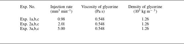The cell is placed vertically, and we were able to install a couple of pressure sensors (TeMaiLong CEIP65, S/N 2025040141) at two distinct locations ( $x_0 \approx \{58,118\}$ cm downstream of the injection point) along the horizontal substrate, as shown in figure 9. A series of gravity current injection experiments were then performed, using glycerine as the working fluid, coloured with food dye (McCormick Assorted), which was injected at different injection rates in a series of new experiments focusing on pressure measurements. In total we performed eight experiments in this set-up, and the experimental parameters are summarised in table 2, including the density, viscosity and injection rate of glycerine for each experiment. The viscosity is measured using a viscometer (SUNLEX, S/N 00000222) at room temperature, and the density of glycerine is also measured using a glass hydrometer. The injection rate is read directly from the pump. In addition, in all experiments, the viscosity and density of air are imposed as $\mu _2 = 1.8 \times 10^{-5}$ Pa s and $\rho _2 = 1.2$ kg m⁻³, respectively, based on standard tables at 20 $^\circ$ C. We also use $g = 9.8$ m s⁻² for gravitational acceleration.

Table 2.

Experimental parameters of gravity current injection into a vertically placed Hele-Shaw cell of gap thickness $d \approx 3.0$ mm. Glycerine was injected as the working fluid, which displaces air. Time evolution of the pressure was measured at two distinct locations along the substrate of the cell. The viscosity and density were measured for glycerine in each experiment, so as the injection rate.

Figure 9.

The experimental set-up of viscous gravity current injection into a vertically-placed Hele-Shaw cell, with two pressure sensors installed along the substrate of the cell, locating at $x_0 \approx \{58,118\}$ cm away from the injection point.

Figure 10.

(a) Time evolution of the measured pressure values at the pressure sensors located at $x_0 \approx \{58,118\}$ cm away from the injection point. Expt. 2a,b,cR indicate pressure data from the second sensor at $x_0 \approx 118$ cm, while the others indicate pressure data from the first sensor at $x_0 \approx 58$ cm. (b) The rescaled and collapsed data points of the measured pressure values in different experiments, along with a comparison with the theoretical prediction (2.7) in the unconfined regime.

Figure 11.

(a) Time evolution of the frontal location as recorded in the experiments, and (b) the rescaled and collapsed data points, along with a comparison with the theoretical prediction $X_{\!f} \sim 1.48\, T^{2/3}$ in the unconfined regime, shown as the solid line.

During each experiment, we can read the pressure values at the monitoring locations directly from the pressure sensors. But we must also subtract the base values before the current’s front arrives at the location of the sensors to obtain the pressure values along the substrate of the Hele-Shaw cell that we are interested in. We then include the experimentally recorded time evolution of the pressure values by the first sensor, which is located at $x_0 \approx 58$ cm away from the injection point, in all performed experiments in figure 10(a). For experiment 2, we also include the pressure values from the second sensor which is located at $x_0 \approx 118$ cm away from the injection point. The measurement error for the pressure sensor is $\pm 4$ Pa and that for time is less than $\pm 1$ s. Both of them are well represented by the size of the symbols, so we did not include additional error bars here. The raw experimental data are also rescaled based on how the theoretical model is non-dimensionalised, and exhibits a very good collapse onto a universal curve, as shown in figure 10(b). The theoretical prediction (2.7) in the unconfined regime is then plotted in the same figure 10(b), and exhibits reasonable agreement with the rescaled experimental data at intermediate times. We must also note that we have imposed a hydrostatic pressure for $p_0(0,t) = \rho _1 g h(0,t)$ as the reference value for the theoretical result (2.7), since we did not install a pressure sensor at the inlet of the cell for technical reasons (there exists an injection channel at $x=0$ ). It is self-consistent to use such a treatment to obtain a comparison between the experimental observations and the theoretical prediction.

As further verifications, we have also provided a comparison between the theoretically predicted and experimentally recorded frontal locations in figure 11(a,b), which shows that these experiments (as described in table 2) lie indeed in the unconfined current regime. Again, the error bars are smaller than the size of the symbols for the raw data, so we did not include them in the figure. There is very good agreement between the theory (i.e. $X_{\!f} \sim 1.48\, T^{2/3}$ ) and experimental observations at intermediate times when the current is sufficiently long. The disagreement at very early times (e.g. when $x_{\!f} \leqslant 10$ cm) is likely due to the influence of wetting and interfacial tension, to our understanding, along with the influence of basal friction. This is also consistent with our discussions of the pressure data for the same experiments.

Overall, we consider that these additional experiments focusing on measuring the pressure evolution help demonstrate that the pressure calculations in the present work could indeed be used to make predictions. Regarding the underlying physics, in these experiments the pressure distribution is indeed hydrostatic at leading order, and its evolution depends on that of the fluid–fluid interface. We are able to make use of previous findings on the profile shape evolution, which leads to useful predictions for the pressure distribution. Otherwise, in the future it would be of interest to perform more experiments to explore the pressure behaviour in the confined regimes. In this case, the inlet pressure $p_0(0,t)$ is no longer the hydrostatic pressure head $\rho _1 g h_0$ , and it would be necessary to obtain this inlet value experimentally, e.g. by installing an additional pressure sensor at the origin.

3.3. Field observations

The model and solutions could possibly find applications in geophysical, environmental and industrial contexts with regard to fluid injection activities into porous reservoirs. In the field, it is typical to track the time evolution of the frontal location of the injecting fluid and the interface shape between the injecting and the ambient fluids based on seismic methods. For example, for geological $\textrm {CO}_2$ sequestration, field data typically well capture the time evolution of the frontal location of a $\textrm {CO}_2$ plume in an aquifer (e.g. Boait et al. Reference Boait, White, Bickle, Chadwick, Neufeld and Huppert2012; Chadwick et al. Reference Chadwick, Williams, Williams and Noy2012; Grude et al. Reference Grude, Landro and Dvorkin2014; Cowton et al. Reference Cowton, Neufeld, White, Bickle, White and Chardwick2016). Nevertheless, to measure the thickness profile of a $\textrm {CO}_2$ plume at higher resolutions, more advanced techniques are required. The present model provides an alternative way to monitor the fate of the injected $\textrm {CO}_2$ within a porous layer based on pressure signals at existing or newly drilled monitoring wells. This seems particularly plausible, considering that there exist many abandoned wells from the petroleum industry during the exploration stage, which often pose risks of greenhouse gas leakage (e.g. Nordbotten et al. Reference Nordbotten, Kavetski, Celia and Bachu2009; Kang et al. Reference Kang, Christian, Celia, Mauzerall, Bill, Miller, Chen, Conrad, Darrah and Jackson2016).

Figure 12.

Field measurements of the BHP at a $\textrm {CO}_2$ sequestration project in the Tubaen Fm., the Snohvit Field, along with the rate of $\textrm {CO}_2$ injection for a period of approximately three years (Grude et al. Reference Grude, Landro and Dvorkin2014). We have observed significant decrease/increase of the BHP when $\textrm {CO}_2$ injection ceases/restarts during the four windows of shut in.

For example, figure 12 presents field data for the evolution of the BHP from a $\textrm {CO}_2$ sequestration project in the Tubaen Fm., the Snohvit Field, along with the rate of $\textrm {CO}_2$ injection (Grude et al. Reference Grude, Landro and Dvorkin2014). Over the period of April 2008–April 2011, more than 1.6 Mt $\textrm {CO}_2$ was injected at the Snohvit Field, which is some $D=2.6$ km (or $D \in [2.56, 2.67]$ km as reported by Grude et al. (Reference Grude, Landro and Dvorkin2014)) underneath the ground surface. While the $\textrm {CO}_2$ injection performance could also be under the influence of rock heterogeneity and salt precipitation (and the injection of chemicals to reduce its influence) for these operations, which are not considered in the present model, we note that there exhibits the general trend of BHP increase upon $\textrm {CO}_2$ injection and BHP decline during the four stages of shut in. In fact, a decline in BHP is typically observed to correlate with a decrease in injection rate (possibly for other reasons) based on these field data. We argue that such a correlation could be explained by the present model. Note that at leading order, the Cartesian configuration mimics the horizontal-well-injection activities such as those at the Sleipner site, while the radial configuration mimics vertical-well injection such as those at the Snohvit Field; see e.g. figure 1 of Eiken et al. (Reference Eiken, Ringrose, Hermanrud, Nazarian, Torp and Hoier2011) for the orientation of the injection wells at the two $\textrm {CO}_2$ sequestration sites. So now we make use of the profile shape $h(r,t)$ and pressure solutions in the radial configuration (e.g. Lyle et al. Reference Lyle, Huppert, Hallworth, Bickle and Chadwick2005; Nordbotten & Celia Reference Nordbotten and Celia2006; Guo et al. Reference Guo, Zheng, Celia and Stone2016b ). In particular, in the original space with dimensions, the background pressure distribution $p_0(r,t)$ along the base ( $y=0$ ) is given by

(3.1) \begin{equation} p(r,0,t) = p(r_i,0,t)- \int _{r_i}^{r} \left [ \frac {Q_{inj}}{2\unicode{x03C0} }\frac { \mu _1 \mu _2}{\hat r k [\mu _2 h + \mu _1 (h_0-h)]} - \frac {\Delta \rho g \mu _1 (h_0-h)}{\mu _2 h + \mu _1 (h_0-h)} \frac {\partial h}{\partial \hat r} \right ]\mathrm{d} \hat r \end{equation}

in a confined porous layer with finite thickness $h_0$ , see also Appendix B, which is used to make predictions in this section. Note that now $p_0(r_i,t)$ is the inlet pressure at the wall of the injection well $r=r_i$ rather than at the origin $r = 0$ . It is necessary to keep this length scale $r_i$ in the radial configuration due to the existence of a pressure singularity as $r \to 0$ .

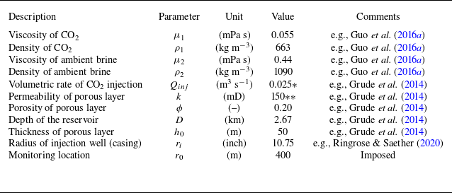
Example calculations are presented in figure 13, where we consider a representative operation of constant fluid injection and shut in that occur alternately along a series of time periods that is consistent with the major trend of figure 12(b). The oscillations of the injection rate $Q_{inj}$ , e.g. due to salt precipitation (as noted by the authors) are neglected, and the imposed $Q_{inj}$ is shown in figure 13(b). We are then able to calculate the BHP evolution based on the present model, as shown in figure 13(a), and indeed we observe the building up of the background pressure upon fluid injection and its decline once injection ceases. Also, the order of magnitude of pressure increase/decrease is found to be consistent with the field data, using geophysical and operational parameters of this project, as summarised in table 3.

Table 3.

Geophysical and operational parameters imposed to obtain the theoretical predictions in figure 13. Gravitational acceleration is imposed as $g = 9.8$ m s⁻ $^2$ . *The corresponding mass rate of injection is approximately 0.53 Mt/yr. **Such an effective permeability is within the range of $k \in [0.01,12\,000]$ mD, as reported by Grude et al. (Reference Grude, Landro and Dvorkin2014).

Figure 13.

An example calculation of the BHP evolution upon fluid injection and shut in that occur alternately as time progresses. The model problem mimics some key features of the operation of figure 12(b), and the results are consistent with the field data in figure 12(a).

It may be of use to provide some further remarks. The thickness of the porous layer is set as $h_0 = 50$ m (e.g. base on figure 1 of Grude et al. Reference Grude, Landro and Dvorkin2014) and the monitoring location is imposed as $r_0 = 400$ m (note that we are not able to find this value from literature), both of which are considered to be reasonable values based on available field data. In the model, the BHP is defined as $\mbox{BHP}(t) \equiv p(r_0,t) = \Delta p(r_0,t) + p_0(0,t)$ , where $\Delta p(r_0,t)$ is the background pressure drop between the origin $r = 0$ and a monitoring location $r = r_0$ , as given by (3.1). The reference pressure $p_0(0,t)$ is defined as the pore pressure at the origin $(r,y)=(0,0)$ that is at depth $D = 2.67$ km underneath the ground surface. In the calculations here, we impose $p_0(0,t) = a\,t^{1/2} + b$ bar where $a = 0.0691$ bar h $^{-1/2}$ and $b = 262$ bar. The value of $b$ corresponds to the hydrostatic pressure of a column of water of length $D = 2.67$ km based on the depth of the reservoir. The additional component of $a\,t^{1/2}$ is imposed to obtain a good match with the field data of BHP evolution in figure 13. Physically, its appearance is likely due to the operation of the pump, but we do not fully understand its exact form.

Overall, these calculations show that it is self-consistent to employ the one-dimensional gravity current models to make estimates on the pressure evolution. In the future, it may be of interest to understand more about the evolution of the reference pressure $p_0(0,t)$ at the injection point under different fluid injection conditions. Once there is a thorough understanding of its evolution, the entire pressure evolution within the porous rock would be known reasonably well based on the present model of the lubrication type and without any fitting parameters. It may also be of interest to explain the observed pressure and injection-rate oscillations by modifying the model appropriately to address the influence of rock heterogeneity, salt precipitation and other related issues.

4.1. Summary

The primary focus of this paper is on the pressure evolution during fluid injections into a horizontal and homogeneous porous layer with finite depth, following a series of previous studies on the interface shape evolution between immiscible fluids during one-dimensional fluid displacement. Understanding the pressure evolution is also useful to evaluate reservoir injectivity, which is important to the success of a subsurface fluid injection activity in practical applications. The model problem here is formulated in the Cartesian configuration and is particularly related to horizontal-well-injection activities, and can be of use to inform practical applications such as geological carbon dioxide sequestration, waste disposal and groundwater management.

For the canonic problem in the Cartesian configuration, previous studies arrived at a nonlinear advective–diffusive PDE to describe the interface shape evolution, while the present work builds upon these efforts to provide further insights into the pressure evolution and fluid injectivity. In particular, the role of two dimensionless parameters were clarified in the dimensionless system that could significantly impact the performance of fluid injections: the viscosity ratio $M \equiv \mu _2/\mu _1$ between the injecting and the ambient fluids, which affects the interface shape evolution (as recognised before), and the relative density difference $G \equiv (\rho _1-\rho _2)/\rho _2$ , which further influences the pressure field evolution within a reservoir (as clarified in this work).

Interestingly, we were also able to obtain self-similar solutions for the background pressure drop $\Delta p_0(x,t) \equiv p(0,t) - p(x,t)$ along the base of the porous layer ( $y=0$ ) in the four different self-similar regimes for the interface shape evolution. In particular, at early times, defined as $t \ll t_c \equiv \Delta \rho gk\phi h_0^3/(\mu _1 q^2)$ , the background pressure drop $\Delta p_0(x,t)$ along the base is very small compared with the hydrostatic pressure head across the thickness of the porous layer, and the pressure drop $\Delta p(x,y,t)$ within the domain varies predominantly in the vertical direction (see e.g. figure 6a ,b). At late times, defined as $t \gg t_c$ , horizontal variations of pressure $\Delta p(x,y,t)$ typically appear due to the influence of the background pressure drop $\Delta p_0(x,t)$ (see e.g. figure 6 c–h). The pressure evolution at specific monitoring locations is also provided at both the early and late times and for different values of $M$ and $G$ . Such information is also of particular use to assess the reservoir injectivity. Laboratory experiments were also performed in a vertically placed Hele-Shaw cell and the pressure data at two specific locations were recorded along the base during the propagation of a viscous gravity current. The pressure data were also rescaled appropriately to collapse onto a universal curve based on the theory, and the collapsed data points show reasonable agreement with the model prediction in the unconfined regime.

The model and solutions could possibly find applications in geophysical, environmental and industrial contexts with regard to fluid injections into porous formations, as we demonstrated in § 3.3 with an example calculation, considering geophysical and operational parameters of a $\textrm {CO}_2$ sequestration project for which field data are available for the BHP and injection-rate evolution. In the field, it is typical to look into the sharp fluid–fluid interface evolution based on seismic methods. The present model provides an alternative way for monitoring the evolution of the injected $\textrm {CO}_2$ plume within a porous layer based on pressure measurements at existing or newly drilled monitoring wells. The solutions and insights obtained for the temporal and spatial evolution of the pressure drop $\Delta p(x,y,t)$ and, in particular, the background pressure drop along the base $\Delta p_0(x,t)$ could be of use for the design of pressure-based monitoring technologies at a well bore. This concept seems particularly plausible, considering that there exist many abandoned wells from the petroleum industry during the exploration stage.

4.2. Assessing reservoir injectivity

The injectivity of a porous reservoir is closely related to the success of a subsurface injection project (e.g. IPCC 2005; Boait et al. Reference Boait, White, Bickle, Chadwick, Neufeld and Huppert2012; Grude et al. Reference Grude, Landro and Dvorkin2014). This could be quantified by the degree of pressure building up at a specific monitoring location and at a specific depth upon fluid injection. This was addressed by the present work in a canonic horizontal configuration in the sharp-interface limit. Our example calculations show that, initially, the background pressure drop $\Delta p_0(x_0,t)$ at a given monitoring location $x = x_0$ would increase with time during the early-time unconfined propagation regime before the arrival of the gravity current’s front (when $x_{\!f}(t) \leqslant x_0$ ). Nevertheless, its evolution becomes non-trivial and depends then on the viscosity ratio $M$ when the propagation becomes confined at intermediate times and the motion of the displaced fluid has to be considered. Our calculations show that, eventually, the background pressure drop $\Delta p_0(x_0,t)$ could decrease with time when the injecting fluid is less viscous or equally viscous compared with the ambient fluid (when $M \geqslant 1$ ), but quite in contrast, $\Delta p_0(x_0,t)$ will continue to increase with time when the injecting fluid is more viscous (when $M \lt 1$ ) until it saturates at a constant value. These findings could also be used to appropriately assess the injectivity of a porous reservoir and also be compared with field measurements to understand the operation and performance.

4.3. The influence of hydrodynamic instabilities

We must note that more attention should be given to the late-time analytical solutions when the injecting fluid is less viscous than the ambient fluid (i.e. when $M\gt 1$ ). This has been recognised indeed when studying the profile shape evolution, which provided a rarefaction solution that depends on the viscosity ratio $M$ (e.g. Zheng et al. Reference Zheng, Guo, Christov, Celia and Stone2015b ). However, for the unfavourable viscosity ratio of $M\gt 1$ , the classic viscous fingering instability (e.g. Saffman & Taylor Reference Saffman and Taylor1958) could possibly develop at intermediate times, and it was found typically that the rarefaction solution over-predicts the location of the propagating front of the injecting fluid, with some two-dimensional numerical evidence provided, e.g. in figure 4 of Nijjer, Hewitt & Neufeld (Reference Nijjer, Hewitt and Neufeld2022), in the regime when fluids mixing is allowed. This is particularly true when the influence of gravity/buoyancy is not significant enough to drive the injecting fluid to propagate along the bottom/top boundary as a gravity current. An interested reader could also refer to the experimental observations in figure 13 of Pegler et al. (Reference Pegler, Huppert and Neufeld2014) when fresh water invades an ambient of (more viscous) syrup solutions in a vertically placed packed-bead Hele-Shaw cell. Correspondingly, with regard to pressure distribution, it is suggested that, when possible (in particular when buoyancy segregation is not significant enough), one should compare the late-time analytical solutions (2.13) and (2.14) with, for example, two-dimensional numerical solutions at representative times, since the propagation could be under the influence of flow instabilities. Currently, we are working on the detailed influence of two-dimensional flow and fluids mixing in this regime.

Finally, quite on the other limit, the fluids can also be immiscible with significant influence of the wetting and capillary effects. Some insights can be obtained within the framework of the generalised Darcy description and under the assumption of vertical gravitational–capillary equilibrium. Previous work suggests that the propagation could also be slowed down when $M\gt 1$ , compared with the prediction of the rarefaction solution; see e.g. figure 3 of Zheng & Neufeld (Reference Zheng and Neufeld2019a ). In this case, the outer profile of the invading fluid develops gradually into a compound-wave shape, with a shock front inserted at $x_{\!f}(t)$ .