



1 Introduction
In the field of number theory, the additive and multiplicative structures of integers are two major areas of research. Multiplicative number theory investigates the distribution of prime numbers through the analysis of generating functions, with the Prime Number theorem and Dirichlet’s theorem being the most famous classical achievements in this field. On the other hand, additive number theory explores the additive decomposition of integers, with the Waring–Goldbach problem being a well-known subject. It has been generally assumed that these two structures are independent, but no proof has confirmed this. Problems involving both structures tend to be more challenging to solve, such as the twin prime conjecture, which asserts that there should be infinitely many pairs of primes which differ by
 $2$
. Although this conjecture remains open, recent work by Zhang [Reference Zhang39], Maynard [Reference Maynard24], Polymath [Reference Polymath27], and many other scholars has made significant progress. Merging both additive and multiplicative aspects within number theory, this article specifically explores coefficients of the standard L-functions over sequences related to the Waring–Goldbach problem.
Let
 $\mathcal {P}$
be the set of all primes, N be a sufficiently large positive integer. Define the sets
 $$ \begin{align*}\mathcal{P}_{k}(N):=\{p\in\mathcal{P}, p^k\le N\},\quad \end{align*} $$
and
 $$ \begin{align*} \mathcal{J}_{k,u}(N):= &\{(p_1, p_2,\dots,p_u)|\ p_i\in \mathcal{P}_{k}(N) ~ (1\le i\le u ), N=p_1^k+p_2^k+\cdots+p_u^k\}, \end{align*} $$
where k and u are positive integers. For a fixed k, the objectives of the Waring–Goldbach problem are to determine the smallest u such that the set
 $\mathcal {J}_{k,u}(N)$
is non-empty and to provide the asymptotic formula for the number of elements in
 $\mathcal {J}_{k,u}(N)$
. We introduce two special cases associated with
 $\mathcal {J}_{k,u}(N)$
: the linear case
 $k=1$
and the quadratic case
 $k=2$
. In both cases, N is assumed to be an odd integer throughout this article.
For
 $k=1$
, Vinogradov [Reference Vinogradov36] proved
 $$ \begin{align*}\# \mathcal{J}_{1,3}(N)=\frac12(1+o(1))\mathfrak{G}_{1,3}(N)\frac{N^2}{(\log N)^{3}}, \end{align*} $$
where
 $\mathfrak {G}_{1,3}(N)$
is the singular series
 $$ \begin{align} \mathfrak{G}_{1,3}(N)=\prod_{p\mid N}\left(1-\frac{1}{(p-1)^{2}}\right)\prod_{p\nmid N}\left(1+\frac{1}{(p-1)^{3}}\right). \end{align} $$
The equation implies that every sufficiently large odd integer N can be expressed as the sum of three primes, representing Vinogradov’s three primes theorem. Furthermore,
 $u=3$
is the minimum number of variables required for
 $\mathcal {J}_{1,u}(N)$
to be non-empty. For the quadratic case
 $k=2$
, and for all sufficiently large N satisfying
 $N\equiv 5\ (\mathrm {mod}\ 24)$
, Hua [Reference Hua15] gave the best result and showed that
 $\#\mathcal {J}_{2,5}(N)>0,$
where the number of variables required is still the best (for more details, see Lemma 7.1).
Inspired by the above result, many scholars have considered the analog of Vinogradov’s three primes theorem for the coefficients of the standard L-functions. Let c be a positive number, whose value may vary throughout the article. Fouvry and Ganguly [Reference Fouvry and Ganguly8] proved that there exists an effective constant
 $c>0$
such that
 $$ \begin{align} \sum_{(p_1,p_2,p_3)\in\mathcal{J}_{1,3}(N)}\nu_f(p_1)\ll_f N^{2} \exp \left(-c\sqrt{\log N}\right), \end{align} $$
where
 $\nu _f (n)$
is the normalized Fourier coefficient of a primitive holomorphic or Maass cusp form f. Let F be a Hecke–Maass form for
 $\mathrm {SL}(3, \mathbb {Z})$
, with
 $A_F(n, 1)$
denoting the nth coefficient of its Dirichlet series. Hou et al. [Reference Hou, Jiang and Lü14] proved that there exists an effective constant
 $c>0$
such that
 $$ \begin{align} \sum_{(p_1,p_2,p_3)\in\mathcal{J}_{1,3}(N)}A_F(p_1, 1) \ll_F N^{2} \exp (-c \sqrt{\log N}). \end{align} $$
For a primitive Dirichlet character
 $\chi $
, Hoffstein and Ramakrishnan [Reference Hoffstein and Ramakrishnan13, Theorem A] and Banks [Reference Banks1] have proved that the twisted L-functions
 $L(s, f\otimes \chi )$
and
 $L(s, F \otimes \chi )$
don’t exist Landau–Siegel zeros. The above two estimates depend on the non-existence of Landau–Siegel zeros. Since the existence of Landau–Siegel zeros is still open for the L-functions with higher ranks, the method used in these results cannot be applied to similar problems for higher ranks. In this article, we introduce a new approach to obtain related estimates for L-functions and Rankin–Selberg L-functions with higher ranks, similar to the estimates (1.2) and (1.3). Moreover, our method can be applied to consider the cancellation of the coefficients associated with the quadratic case, which is more intricate. Inspired by the approach for handling the Waring–Goldbach problem, we employ several different estimates of exponential sums to obtain the optimal upper bound (for more details, see Section 5.3).
Let
 $\mathbb {A}$
be the ring of adeles over
 $\mathbb {Q}$
. Define a unitary Hecke character
 ${\omega : \mathbb {Q}^{\times }\backslash \mathbb {A}^{\times } \rightarrow \mathbb {C}^{\times }}$
. Consider the set
 $$\begin{align*}\mathfrak{E}_m:=\{\pi \subset L^{2}(\mathrm{GL}_{m}(\mathbb{Q}) \backslash \mathrm{GL}_{m}(\mathbb{A}); \omega) \mid \omega \text{ is trivial, }\pi \text{ is irreducible and cuspidal} \}. \end{align*}$$
Given
 $\pi \in \mathfrak {E}_m$
, let
 $\mathfrak {q}_\pi $
be the conductor of
 $\pi $
,
 $L(s, \pi )$
be the associated standard L-function, and
 $\widetilde {\pi } \in \mathfrak {E}_m$
be the contragredient representation. We write
 $\lambda _\pi (n)$
to be the nth Dirichlet coefficient of
 $L(s, \pi )$
. Let
 $\chi $
be a Hecke character of the idele class group
 $\mathbb {Q}^{\times }\backslash \mathbb {A}^{\times } $
. We define the set
 $$ \begin{align*}\begin{aligned} \mathfrak{E}_m^b:=\{\pi \in \mathfrak{E}_m&|\pi=\widetilde{\pi} \text{ and } \pi \neq \pi \otimes \chi \\& \text{ for all non-trivial primitive quadratic Dirichlet characters }\chi\}. \end{aligned}\end{align*} $$
We will examine the cancellation of the multiplicative Dirichlet coefficients
 $\lambda _{\pi }(n)$
over specific sequences
 $\mathcal {J}_{1,3}(N)$
and
 $\mathcal {J}_{2,5}(N)$
, and provide some applications.
Theorem 1.1 Let
 $\pi \in \mathfrak {E}_m^b$
and
 $B>0$
be a sufficiently large constant. Then
 $$ \begin{align*}r_\pi(N):=\sum_{(p_1,p_2,p_3)\in\mathcal{J}_{1,3}(N)} \lambda_{\pi}\left(p_1\right) \ll_{\pi, B} N^{2}(\log N)^{-B}, \end{align*} $$
and
 $$ \begin{align*}w_\pi(N):=\sum_{(p_1,p_2,p_3,p_4,p_5)\in\mathcal{J}_{2,5}(N)} \lambda_{\pi}\left(p_1\right) \ll_{\pi, B} N^{3/2}(\log N)^{-B}.\end{align*} $$
Due to the potential existence of these zeros, the bounds in the above theorem are weaker than those in (1.2) and (1.3), and the condition
 $\pi \in \mathfrak {E}_{m}^{b}$
is required to obtain Theorem 1.1. Assuming an enhanced zero-free region for
 $\pi \in \mathfrak {E}_{m}$
, sharper upper bounds can be derived for a broader class of L-functions.
Hypothesis S Let
 $1/2\le \delta <1$
. For any
 $\pi \in \mathfrak {E}_m$
with
 $m\ge 1$
, the L-functions
 $L(s,\pi )$
have no zeros for
 $\mathrm {Re}(s)>\delta $
.
Theorem 1.2 Let
 $\pi \in \mathfrak {E}_m$
and
 $\varepsilon $
be a sufficiently small positive number. Under Hypothesis S,
 $$ \begin{align*}r_\pi(N) \ll_{\varepsilon} m^{2} N^{\frac{5}{3}+\frac{\delta}{3}+\varepsilon}(\log (N \mathfrak{q}_{\pi}))^3, \end{align*} $$
and
 $$ \begin{align*}w_\pi(N) \ll_{\varepsilon} m^{2} (N^{\frac{23}{16}+\varepsilon}+N^{\frac{4}{3}+\frac{\delta}{6}+\varepsilon})(\log( N\mathfrak{q}_{\pi}))^{3}. \end{align*} $$
Remark
-
(1) Regarding the upper bounds in (1.2) and (1.3), we can use the same method as in Theorem 1.2 to obtain them.
-
(2) Note that the upper bound for
 $w_\pi (N)$
consists of two terms. This is due to the use of Dirichlet approximation theorem, which allows us to divide the minor arcs twice. Such an approach is effective in handling minor arcs within the circle method.

In our above cases, we do not provide asymptotic formulas. But the upper bounds we obtain are better than the error terms in the classical cases (see Lemma 7.1). Furthermore, we utilize the relationship between the Rankin–Selberg L-function and the adjoint L-function to obtain asymptotic formulas concerning the Rankin–Selberg coefficients over
 $\mathcal {J}_{k,u}(N)$
. For
 $\pi \in \mathfrak {E}_m$
, the construction of an adjoint L-function is described by employing a Rankin–Selberg L-function and zeta function:
 $$ \begin{align} L(s, \operatorname{Ad}\pi):=\frac{L(s, \pi \times \tilde{\pi})}{\zeta(s)}, \end{align} $$
where
 $\operatorname {Ad}\pi $
is the adjoint lift of
 $\pi $
. The adjoint L-function is meromorphic since
 $L(s, \pi \times \widetilde {\pi })$
and
 $\zeta (s)$
are meromorphic. Details regarding the Rankin–Selberg L-functions can be found in Section 2. For
 $\mathrm {Re}(s)>1$
, we express
 $$ \begin{align*}L(s, \operatorname{Ad}\pi)=\prod_p \underset{ (i, j) \neq (1,1)}{\prod_{i=1}^m\prod_{j=1}^{m}}\left(1-\frac{\alpha_{i, \pi}(p)\overline{\alpha_{j, \pi}(p)}}{p^s}\right)^{-1}=\sum_{n=1}^{\infty} \frac{\lambda_{\operatorname{Ad}\pi}(n)}{n^{s}}. \end{align*} $$
By the relation between
 $\lambda _{\pi \times \widetilde {\pi }}(p)$
and
 $\lambda _{\operatorname {Ad}\pi }(p)$
, we easily obtain the following results.
Corollary 1.3 Let
 $\pi \in \mathfrak {E}_m^b$
,
 $\varepsilon $
be a sufficiently small positive number and
 $B>0$
be a sufficiently large constant.
-
(1) Under the hypothesis that
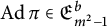
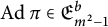
$\operatorname {Ad}\pi \in \mathfrak {E}_{m^{2}-1}^b$
, and
$$ \begin{align*}r_{\pi\times\tilde{\pi}}(N):=\sum_{(p_1,p_2,p_3)\in\mathcal{J}_{1,3}(N)} \lambda_{\pi\times\tilde{\pi}}\left(p_1\right) =\# \mathcal{J}_{1,3}(N)+O_{\pi,B}(N^{2}(\log N)^{-B}),\end{align*} $$
$$ \begin{align*}w_{\pi\times\tilde{\pi}}(N):=\sum_{(p_1,p_2,p_3,p_4,p_5)\in\mathcal{J}_{2,5}(N)} \lambda_{\pi\times\tilde{\pi}}\left(p_1\right) =\# \mathcal{J}_{2,5}(N)+O_{\pi,B}(N^{2}(\log N)^{-B}). \end{align*} $$
-
(2) Under Hypothesis S and the hypothesis that
$\operatorname {Ad}\pi \in \mathfrak {E}_{m^{2}-1}^b$
, and
$$ \begin{align*}r_{\pi\times\tilde{\pi}}(N) =\# \mathcal{J}_{1,3}(N)+O_{\varepsilon}(m^{2}N^{\frac{5}{3}+\frac{\delta}{3}+\varepsilon}(\log ( N\mathfrak{q}_{\pi}))^3),\end{align*} $$
$$ \begin{align*}w_{\pi\times\tilde{\pi}}(N) =\# \mathcal{J}_{2,5}(N)+O_{\varepsilon}(m^{2}(N^{\frac{23}{16}+\varepsilon}+N^{\frac{4}{3}+\frac{\delta}{6}+\varepsilon })(\log ( N\mathfrak{q}_{\pi}))^3).\end{align*} $$




Remark Following from Lemma 7.1 in Appendix, we note that if N satisfies some necessary congruence conditions, then
 $\# \mathcal {J}_{1,3}(N)\asymp N^2/(\log N)^{3}$
and
 $\# \mathcal {J}_{2,5}(N)\asymp N^{3/2}/(\log N)^{5}$
which are the main terms in the above asymptotic formulas.
We have made a hypothesis regarding the automorphy of
 $\operatorname {Ad}\pi $
in the above corollary. In the following remark, we have presented several cases that meet the hypothesis.
Remark
-
(1) If
$m=2$
, the adjoint lift of
$\pi $
is automorphic. Furthermore,
$\operatorname {Ad} \pi $
is cuspidal if and only if
$\pi $
is not an automorphic induction of a Hecke character according to [Reference Gelbart and Jacquet10]. For
$m>2$
, the conjecture that the adjoint lift of
$\pi $
is automorphic is widely open. -
(2) For a positive integer
$N_1$
and an even positive integer
$k_{1}$
, we denote by
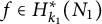
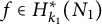
$H_{k_{1}}^*(N_1)$
the finite set of all primitive cusp forms of weight
$k_{1}$
with trivial nebentypus for the Hecke congruence group
$\Gamma _0(N_1)$
. Each
$f \in H_{k_{1}}^*(N_1)$
has a Fourier expansion in the upper half-plane. It is known that Newton and Thorne [Reference Newton and Thorne25, Reference Newton and Thorne26] have proven that
$$\begin{align*}f(z)=\sum_{n=1}^{\infty} \lambda_f(n) n^{\frac{k_{1}-1}{2}} e(n z) \end{align*}$$
$ \mathrm {sym}^{j}f$
corresponds to
$ \mathrm {sym}^j \pi _{f}$
, which is a cuspidal automorphic representation of
$\mathrm {GL}_{j+1}$
over
$\mathbb {Q}$
for all
$j\ge 1$
. Using well-known identities: for all
$j \ge 1$
, and
$$\begin{align*}\mathrm{sym}^2\left(\mathrm{sym}^j \pi_{f}\right)=\bigoplus_{0 \le i \le j / 2} \mathrm{sym}^{2 j-4 i} \pi_{f} \quad \text{(see }[9, \text{ Page }159]) \end{align*}$$
where
$$ \begin{align*} \left(\mathrm{sym}^j \pi_{f}\right)^{\otimes 2}:=\mathrm{sym}^j \pi_{f} \otimes \mathrm{sym}^j \pi_{f}=\bigoplus_{0 \le r \le j} \mathrm{sym}^{2 r} \pi_{f} \quad \text{(see }[9, \text{ Page }151]), \end{align*} $$
$\mathrm {sym}^0 \pi _{f}$
is the
$1$
-dimensional trivial representation, we have In this case,
$$ \begin{align*} \operatorname{Ad}\mathrm{sym}^j \pi_{f}=\bigoplus_{1 \le r \le j} \mathrm{sym}^{2 r} \pi_{f}.\end{align*} $$
$\operatorname {Ad}\mathrm {sym}^j \pi _{f}$
is cuspidal and automorphic.
-
(3) When
$m = 2$
and
$\mathrm {sym}^{j}\pi $
represents the jth symmetric power of the standard representation of
$\mathrm {GL}_2$
, the automorphy of
$\mathrm {sym}^{j}\pi $
was established for
$j = 2$
by Gelbart and Jacquet [Reference Gelbart and Jacquet10], and for
$j = 3, 4$
by Kim and Shahidi [Reference Kim and Shahidi21, Reference Kim and Shahidi22]. Similar to (2),
$\operatorname {Ad}\mathrm {sym}^{2}\pi $
is also automorphic.




As an application, we present an analog of the Sato–Tate conjecture. We restrict our analysis to forms with trivial nebentypus, ensuring that all Fourier coefficients are real. Additionally, we assume that
 $f\in H_{k_{1}}^*(N_1)$
does not possess complex multiplication (CM), meaning there is no imaginary quadratic field K such that for
 $p \nmid N_1$
,
 $ p$
is inert in K if and only if
 $\lambda _f(p)=0$
. Deligne’s proof of the Weil conjectures [Reference Deligne7] implies that for each prime p, there exists an angle
 $\theta _p \in [0, \pi ]$
such that
 $\lambda _f(p)=2 \cos \theta _p$
. The Sato–Tate conjecture asserts that if
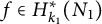 $f\in H_{k_{1}}^*(N_1)$
is non-CM, then the sequence
 $\left \{\theta _p\right \}$
is equidistributed in the interval
 $[0, \pi ]$
with respect to the measure
 $$ \begin{align*}\mathrm{d} \mu_{\mathrm{ST}}:=(2 / \pi) \sin ^2 \theta \mathrm{d} \theta.\end{align*} $$
Equivalently, we obtain that
 $$ \begin{align} \pi_{f, I}(x):=\#\left\{p \le x: \theta_p \in I, p \nmid N_1\right\} \sim \mu_{\mathrm{ST}}(I) \pi(x) \quad \text { as } x \rightarrow \infty, \end{align} $$
where
 $\pi (x)=\#\{p \le x\}$
and
 $I=[\alpha , \beta ] \subseteq [0, \pi ]$
. Barnet-Lamb et al. [Reference Barnet-Lamb, Geraghty, Harris and Taylor2] proved the Sato–Tate conjecture. For all primitive characters
 $\chi $
, Thorner [Reference Thorner34] has proved that the twisted L-functions
 $L(s,\mathrm {sym}^{j}f\otimes \chi )$
have no Landau–Siegel zeros. Based on this property, we will show that the equidistribution of
 $\theta _{p_1}$
remains undisturbed over the set
 $\mathcal {J}_{1,3}(N)$
. Moreover, as an application of Theorem 1.2, we will also investigate the distribution of
 $\lambda _{f}(p_{1})$
associated with
 $(p_1,p_2,p_3)$
in the set
 $\mathcal {J}_{1,3}(N)$
under Hypothesis S. We define
 $$\begin{align*}\mathcal{J}_{1,3,f, I}(N):=\{(p_1,p_2,p_3)\in \mathcal{J}_{1,3}(N) : \theta_{p_1} \in I, p_1 \nmid N_1\}. \end{align*}$$
Theorem 1.4 Fix a non-CM form
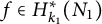 $f\in H_{k_{1}}^*(N_1)$
.
-
(1) If
$N_1$
is squarefree, then If
$$ \begin{align*}\# \mathcal{J}_{1,3,f, I}(N) =\mu_{\mathrm{ST}}(I)\left(\# \mathcal{J}_{1,3}(N)\right)+O\left(\frac{\log (k_1 N_1 \log N)}{ (\log N)^{1/2} }\left(\# \mathcal{J}_{1,3}(N)\right)\right). \end{align*} $$
$N_1$
is not squarefree, then
$$ \begin{align*}\# \mathcal{J}_{1,3,f, I}(N) =\mu_{\mathrm{ST}}(I)\left(\# \mathcal{J}_{1,3}(N)\right)+O\left(\frac{\log (k_1 N_1 \log N)}{ (\log N)^{1/4} }\left(\# \mathcal{J}_{1,3}(N)\right)\right). \end{align*} $$
-
(2) Under Hypothesis S, we have
$$ \begin{align*}\# \mathcal{J}_{1,3,f, I}(N) =\mu_{\mathrm{ST}}(I)\left(\# \mathcal{J}_{1,3}(N)\right)+O(N^{11/6+\delta/6}(\log N)^{3}).\end{align*} $$


It follows from the above result and (1.5) that
 $$ \begin{align} \frac{\# \mathcal{J}_{1,3,f, I}(N)}{\# \mathcal{J}_{1,3}(N)} \sim \frac{\pi_{f, I}(N)}{\pi(N)} \quad \text { as } N \rightarrow \infty. \end{align} $$
From a different perspective, it follows from (1.6) and Lemma 7.1 that
 $$ \begin{align} \frac{\# \mathcal{J}_{1,3,f, I}(N)}{ \pi_{f, I}(N)}\sim\frac{\# \mathcal{J}_{1,3}(N)}{\pi(N)}\sim \frac{\mathfrak{G}_{1,3}(N)N}{2(\log N)^{2}}\quad \text { as } N \rightarrow \infty. \end{align} $$
The Goldbach conjecture states that every even number
 $2N$
can be expressed as the sum of two odd primes. Hardy and Littlewood [Reference Hardy and Littlewood11] conjectured an asymptotic formula for the number of such representations as follow:
 $$ \begin{align} \#\mathcal{J}_{1,2}(2N)\sim2 C_2 \frac{2N}{(\log 2N)^2} \prod_{\mathfrak{p}}\left(\frac{\mathfrak{p}-1}{\mathfrak{p}-2}\right), \end{align} $$
where
 $\mathfrak {p}$
is an odd prime divisor of
 $2N$
, and
 $$ \begin{align*}C_2=\prod_{\varpi=3}^{\infty}\left(1-\frac{ 1}{(\varpi-1)^2}\right) .\end{align*} $$
Comparing the result (1.7) with the conjecture (1.8), it seems that the condition
 $\theta _{p_1} \in I$
does not affect the selection of
 $p_2$
and
 $p_3$
in
 $\mathcal {J}_{1,3}(N)$
. Building on results from the Waring–Goldbach problem, it is observed that each
 $p_i$
(
 $1\le i \le k-1$
) in
 $\mathcal {J}_{k,u}(N)$
covers almost all primes. This suggests that the behavior of these sums, particularly in the context of Goldbach-type problems, can be analyzed probabilistically. Thus, we propose to approach the Goldbach conjecture from a probabilistic perspective, wherein the selection of primes in such sums can be viewed as random variables following certain statistical distributions.
Define the set
 $$ \begin{align*}\Omega:=\{&(1,1,N-2),(1,2,N-3),\dots,(1,N-2,1),(2,1,N-3),\\&(2,2,N-4),\dots,(2,N-3,1),\dots,(N-3,1,2),(N-3,2,1),(N-2,1,1)\}.\end{align*} $$
Let
 $\mathcal {F}$
be the set of all subsets of
 $\Omega $
and
 $\phi $
be an empty set. According to [Reference Yong and Zhou38, Chapter 1],
 $(\Omega , \mathcal {F})$
forms a measurable space. Let
 $\mathbf {P}$
be a map:
 $\mathcal {F} \rightarrow [0,1]$
, which is a probability measure on
 $(\Omega , \mathcal {F})$
satisfying
 $$ \begin{align*}\left\{\begin{array}{@{}c} \mathbf{P}(\phi)=0, \quad \mathbf{P}(\Omega)=1,\\ A_i \in \mathcal{F}~( i=1,2, \dots, 2^{\# \Omega}), \quad \mathbf{P}\left( A_i\right)=\frac{\# A_i}{\# \Omega}. \end{array}\right. \end{align*} $$
The triple
 $(\Omega , \mathcal {F}, \mathbf {P})$
forms a probability space. We denote two events
 $$ \begin{align*}A:=\{ (p_1,n_2,n_3)|p_1 \in \mathcal{P}, n_2,n_3 \in \mathbb{N}, N=p_1+n_2+n_3 \} \end{align*} $$
and
 $$ \begin{align*}A^{\prime}:=\{ (n_1,p_2,p_3)|n_1 \in \mathbb{N}, p_2,p_3 \in \mathcal{P}, N=n_1+p_2+p_3 \}. \end{align*} $$
It is evident that
 $A \cap A^{\prime }$
is the set
 $\mathcal {J}_{1,3}(N)$
. Inspired by (1.7), we propose an interesting conjecture related to the Goldbach conjecture.
Conjecture 1.5 As for
 $(\Omega , \mathcal {F}, \mathbf {P})$
, the events A and
 $A^{\prime }$
satisfy
 $$ \begin{align*}\mathbf{P}(A \cap A^{\prime})\sim \mathbf{P}(A)\mathbf{P}(A^{\prime}). \end{align*} $$
By the Prime Number theorem and Lemma 7.1, when N is a sufficiently large odd integer, we derive that
 $$ \begin{align*}\mathbf{P}(A)\sim\frac{1}{\log N},\quad\quad \mathbf{P}(A\cap A^{\prime})\sim\frac{\mathfrak{G}_{1,3}(N)}{(\log N)^{3}}.\end{align*} $$
Under Conjecture 1.5,
 $$ \begin{align*}\mathbf{P}(A^{\prime})\sim\frac{\mathbf{P}(A \cap A^{\prime})}{\mathbf{P}(A)}\sim\frac{\mathfrak{G}_{1,3}(N)}{(\log N)^{2}}. \end{align*} $$
Since the number of samples in
 $\Omega $
is given by
 $(N^{2}-3N+2)/2$
, we can conclude that
 $$ \begin{align}\# A^{\prime}\sim\frac{\mathfrak{G}_{1,3}(N)N^{2}}{2 (\log N)^{2}}.\end{align} $$
Also, we calculate the number of the samples in
 $A^{\prime }$
, that is,
 $$ \begin{align} \#\mathcal{J}_{1,2}(N-4)+\#\mathcal{J}_{1,2}(N-5)+\dots+\#\mathcal{J}_{1,2}(4). \end{align} $$
It follows from (1.9) and a rough estimate that
 $$ \begin{align} \sum_{n=2}^{(N-5)/2}\#\mathcal{J}_{1,2}(2n)\sim \frac{\mathfrak{G}_{1,3}(N)N^{2}}{2(\log N)^{2}}. \end{align} $$
If Conjecture 1.5 holds, we would obtain the estimate (1.11), which shows that the Goldbach conjecture is right on average.
Remark For (1.10), we can apply the asymptotic formula (1.8) to derive a more precise estimate:
 $$\begin{align*}\sum_{n=2}^{(N-5)/2} 2 C_2 \frac{2n}{(\log 2n)^2} \prod_{\mathfrak{p}}\left(\frac{\mathfrak{p}-1}{\mathfrak{p}-2}\right). \end{align*}$$
Comparing this result with (1.11), we see that Conjecture 1.5 provides additional support for the validity of the asymptotic formula (1.8).
Structure of this article. The structure of this article is outlined as follows. In Section 2, we present two important propositions that are used to prove our main theorems. In Section 3, we provide some fundamental definitions and properties of L-functions along with several useful lemmas. Section 4 is dedicated to the proofs of Propositions 2.1 and 2.2, leveraging the Rankin–Selberg results, the Mellin transform, and the functional equations of L-functions. In Section 5, we establish Theorems 1.1 and 1.2 by employing the Hardy–Littlewood circle method in conjunction with Propositions 2.1 and 2.2. In Section 6, an analog of the Sato–Tate conjecture is presented as an application of the methods used in Theorem 1.2, denoted as Theorem 1.4. Finally, Section 7 provides several useful appendices.
In this article, we investigate the apparent oscillatory properties of
 $\lambda _{\pi }(n)$
in its interactions with the additive structure of integers. For example, in Theorem 1.4, we observe that the equidistribution of the sequence
 $\theta _p$
in the interval
 $[0, \pi ]$
remains unaffected by the additive structure of integers associated with the Waring–Goldbach problem. We hope that the ideas presented in this article (particularly the combination of concepts from both additive and multiplicative problems) may inspire further applications and advancements in related areas of research.
2 Exponential estimates
In relation to the Waring–Goldbach problem, we will utilize the Hardy–Littlewood circle method. This method involves transforming a discrete weighted sum into an integral over
 $[0,1)$
with respect to related exponential sums such as
 $$ \begin{align} \sum_{n \le x} \Lambda(n) a(n) e\left(n^k \alpha\right), \end{align} $$
where
 $a(n)$
is an arithmetic function and
 $\alpha \in [0,1)$
. Estimating such exponential sums is key to solve the problem. For example, Fouvry and Ganguly [Reference Fouvry and Ganguly8] obtained
 $$ \begin{align} \sum_{n \le x} \Lambda(n) \nu_f(n) e(n \alpha) \ll_{f} x \exp (-c \sqrt{\log x}), \end{align} $$
which was used in the proof of (1.2). Hou et al. [Reference Hou, Jiang and Lü14] got
 $$ \begin{align} \sum_{n \le x} \Lambda(n) A_F(n, 1) e(n \alpha) \ll_F x \exp (-c \sqrt{\log x}) \end{align} $$
to prove (1.3). The non-existence of Landau–Siegel zeros plays an important role in estimating the sums (2.2) and (2.3).
In this article, instead of relying on the non-existence of Landau–Siegel zeros in the twisted L-functions, we consider the sum (2.1) for high ranks. Let
 $\mathbb {T}$
denote the torus
 $\mathbb {Z} \backslash \mathbb {R}$
, and identify
 $\mathbb {T}$
with the unit interval
 $[0, 1)$
throughout this article. For any
 $\alpha \in \mathbb {T}$
, we provide estimates of (2.1) with
 $a(n) = \lambda _{\pi }(n)$
that do not depend on the generalized Ramanujan conjecture (GRC, as described in Section 3) or on the non-existence of Landau–Siegel zeros in the twisted L-functions. This is the first time such estimates have been obtained.
Proposition 2.1 Let
 $\pi \in \mathfrak {E}_m^b$
. For any real number
 $\alpha \in \mathbb {T}$
, suppose that there exist two integers a and q, such that
 $$ \begin{align*}\alpha=a/q +\lambda, \ \ |\lambda|\le \frac{1}{qQ}, \ \ (a,q)=1,\ \ 1\le q\le Q\le x^{k}, \end{align*} $$
where Q is a large positive integer. For all
 $A>0$
, if
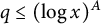 $q\le (\log x)^{A}$
, then
 $$ \begin{align*}\sum_{p\le x}\lambda_{\pi}(p)e(p^{k}\alpha)\log p\ll_{\pi,A} \bigg(1+\frac{x^{k}}{qQ}\bigg)q^{\frac{m+1}{2}}x \exp \left(-c \sqrt{\log x}\right), \end{align*} $$
where c is an ineffective constant depending on A and
 $\pi $
.
Proposition 2.2 Let
 $\pi \in \mathfrak {E}_m$
,
 $\varepsilon $
be a sufficiently small positive number. For any real number
 $\alpha \in \mathbb {T}$
, suppose that there exist two integers a and q, such that
 $$ \begin{align*}\alpha=a/q +\lambda, \ \ |\lambda|\le \frac{1}{qQ}, \ \ (a,q)=1,\ \ 1\le q\le Q, \end{align*} $$
where Q is a large positive integer. Under Hypothesis S,
 $$ \begin{align*}\sum_{p\le x}\lambda_{\pi}(p)e(p^{k}\alpha)\log p\ll m^{2}\bigg(1+\frac{x^{k}}{qQ}\bigg)q^{\frac{1}{2}}x^{\delta+\varepsilon}(\log (x \mathfrak{q}_{\pi})) ^{3}+x^{\frac34}. \end{align*} $$
Remark Compared to similar results previously, Proposition 2.2 states the relation between the upper bound of the exponential sum concerning
 $\lambda _{\pi }(p)$
and
 $\pi $
for the first time.
Our new approach can be applied not only to derive (1.2) and (1.3), but also to extend similar results to higher ranks. Consider Dirichlet rational approximation, where there exist integers a and q such that
 $$ \begin{align} \alpha = \frac{a}{q} + \lambda, \quad |\lambda| \le \frac{1}{qQ}, \quad (a, q) = 1, \quad 1 \le q \le Q, \end{align} $$
for any
 $\alpha \in \mathbb {T}$
, with Q being a large positive integer. When
 $\alpha $
is in intervals around rational numbers
 $a/q$
with large denominators (i.e., in the so-called minor arcs), we can apply results for the following exponential sums (refer to Lemmas 5.1–5.3 below):
 $$\begin{align*}\sum_{m \le x} \Lambda(m) e\left(m^k \alpha\right), \end{align*}$$
where x is a large real number. In contrast, when
 $\alpha $
lies in the major arcs, we use Propositions 2.1 and 2.2. By employing two distinct estimations, one for the major arcs and the other for the minor arcs, we can bypass the limitations of previous methods in such problems, thereby obtaining Theorems 1.1 and 1.2.
3 Background on L-functions
3.1 Standard L-functions
Let
 $m \ge 1$
be an integer. Fix
 $\pi =\otimes _{p} \pi _{p} \in \mathfrak {E}_{m}$
, where p ranges over all primes. The standard function
 $L(s, \pi )$
is given by the Dirichlet series
 $$ \begin{align} \begin{aligned} L(s, \pi) &=\prod_p L(s,\pi_{p})=\sum_{n=1}^{\infty} \frac{\lambda_\pi(n)}{n^s},\end{aligned} \end{align} $$
with both the series and the product converging absolutely for
 $\mathrm {Re}(s)>1$
. For each p, the local factor
 $L(s,\pi _{p})$
is defined in terms of Satake parameters
 $\{\alpha _{1,\pi }(p),\dots ,\alpha _{m,\pi }(p)\}$
by
 $$ \begin{align*}L(s,\pi_{p}):= \prod_{j=1}^m\left(1-\frac{\alpha_{j, \pi}(p)}{p^s}\right)^{-1}=\sum_{i=0}^{\infty} \frac{\lambda_\pi\left(p^i\right)}{p^{is}}. \end{align*} $$
Let
 $\mathfrak {q}_{\pi }$
denote the conductor of
 $\pi $
. For
 $1\le j\le m$
, we have
 $\alpha _{j,\pi }(p)\neq 0$
when
 $p\nmid \mathfrak {q}_{\pi }$
. When
 $p\mid \mathfrak {q}_{\pi }$
, the case might be that
 $\alpha _{j,\pi }(p)=0$
. At the archimedean place of
 $\mathbb {Q}$
, there exist m complex Langlands parameters
 $\mu _{\pi }(j)$
, from which we define the Dirichlet series
 $$ \begin{align} L_{\infty}(s, \pi):=\pi^{-m s / 2} \prod_{j=1}^m \Gamma\left(\frac{s+\mu_\pi(j)}{2}\right). \end{align} $$
Let
 $\tilde {\pi }$
denote the contragredient representation of
 $\pi \in \mathfrak {E}_m$
, which is also an irreducible cuspidal automorphic representation in
 $\mathfrak {E}_m$
. For each
 $p \le \infty $
, we have the following equations
 $$ \begin{align*}\big\{\alpha_{j, \tilde{\pi}}(p):1\le j\le m\big\}=\big\{\overline{\alpha_{j, \pi}(p)}:1\le j\le m\big\} \end{align*} $$
and
 $$ \begin{align*}\big\{\mu_{\tilde{\pi}}(j):1\le j\le m\big\}=\big\{\overline{\mu_\pi(j)}:1\le j\le m\big\}. \end{align*} $$
For a non-trivial
 $\pi $
, the complete L-function is defined by
 $$ \begin{align*}\Lambda(s, \pi):=\mathfrak{q}_{\pi}^{\frac{s}{2}} L(s, \pi) L_{\infty}(s, \pi). \end{align*} $$
The complete L-function
 $\Lambda (s, \pi )$
has an analytic continuation to the entire complex plane, and is of finite order. Moreover, it satisfies the functional equation
 $$ \begin{align*}\Lambda(s, \pi)=W_{\pi} \Lambda(1-s, \tilde{\pi}), \end{align*} $$
where
 $W_{\pi }$
is the root number (a complex number of magnitude
 $1$
). For all primes p and
 $1 \le j \le m$
, it follows from [Reference Kim20]
 $(2 \le m \le 4)$
and [Reference Luo, Rudnick and Sarnak23]
 $(m \ge 5)$
that the best known bound is
 $$ \begin{align*}\left|\alpha_{j, \pi}(p)\right| \le p^{\theta_{m}} \quad \text { and } \quad -\mathrm{Re}(\mu_{\pi}(j))\le \theta_{m}, \end{align*} $$
where
 $$ \begin{align} \theta_{2}=\frac{7}{64}, \quad \theta_{3}=\frac{5}{14}, \quad \theta_{4}=\frac{9}{22}, \quad \theta_{m}=\frac{1}{2}-\frac{1}{m^{2}+1}\ (m \ge 5). \end{align} $$
The GRC predicts that
 $$ \begin{align*}\theta_{m}=0\end{align*} $$
for all
 $m\ge 1.$
The analytic conductor of
 $\pi $
is defined by
 $$ \begin{align} C(\pi, t):=\mathfrak{q}_{\pi} \prod_{j=1}^{m}\left(1+\left|i t+\mu_{\pi}(j)\right|\right), \quad C(\pi):=C(\pi, 0). \end{align} $$
Taking the logarithmic derivative for
 $L(s, \pi )$
, we obtain that for
 $\mathrm {Re}(s)>1$
,
 $$ \begin{align*}-\frac{L^{\prime}}{L}(s, \pi)=\sum_{p} \sum_{k=1}^{\infty} \frac{a_{\pi} (p^k) \log p}{p^{k s}}=\sum_{n=1}^{\infty} \frac{a_\pi(n) \Lambda(n)}{n^s}, \end{align*} $$
where
 $$ \begin{align} a_\pi\left(p^k\right)=\sum_{j=1}^m \alpha_{j, \pi}(p)^k. \end{align} $$
Lemma 3.1 Let
 $\pi \in \mathfrak {E}_{m}$
,
 $m\ge 2$
, and
 $\varepsilon $
be a sufficiently small positive number.
-
(1) Under Hypothesis S,
(3.6)
$$ \begin{align} \sum_{n\le x} \Lambda(n)a_{\pi}(n) \ll_{\varepsilon} mx^{\delta+\varepsilon} (\log x)^{2} \log \mathfrak{q}_{\pi}. \end{align} $$
-
(2) Under Hypothesis S and GRC, the upper bound is improved to
(3.7)
$$ \begin{align} \sum_{n\le x} \Lambda(n)a_{\pi}(n) \ll x^{\delta}(\log x)^{2}(\log \log (x^{m} C(\pi)))^{2}. \end{align} $$


Proof Let y be a parameter satisfying the inequality
 $1 \le y \le x$
, will be determined later. Denote
 $\phi (z)$
as the function with support on the interval
 $[0, x+y]$
, satisfying the conditions
 $\phi (z)=1$
for
 $1 \le z \le x$
, and
 $|\phi (z)| \le 1$
elsewhere. By the Cauchy–Schwarz inequality, (3.15) and the Prime Number theorem in short intervals [Reference Huxley17], we can achieve a smoother expression by writing
 $$ \begin{align} \sum_{n\le x} \Lambda(n)a_{\pi}(n)=\sum_n \Lambda(n)a_{\pi}(n) \phi(n)+O(\sqrt{x y}), \quad x^{7/12}\ll y\ll x. \end{align} $$
For
 $0 \le z \le x+y$
, we take
 $$ \begin{align*}\phi(z)=\min \left(\frac{z}{y}, 1,1+\frac{x-z}{y}\right) \end{align*} $$
and set
 $\phi (z)=0$
for
 $z>x+y$
. The Mellin transform of
 $\phi (z)$
satisfies
 $$ \begin{align*}\hat{\phi}(s)=\int_0^{x+y} \phi(z) z^{s-1} \mathrm{d} z \ll \frac{x^\sigma}{|s|} \min \left(1, \frac{x}{|s| y}\right) \end{align*} $$
for
 $s=\sigma +i t, \frac {1}{2} \le \sigma \le 2$
. The sum on the right-hand side of (3.8) can be expressed as
 $$ \begin{align*}\sum_n \Lambda(n)a_{\pi}(n) \phi(n)=\frac{1}{2 \pi i} \int_{(2)}-\frac{L^{\prime}}{L}(s, \pi) \hat{\phi}(s) \mathrm{d} s, \end{align*} $$
where the integral converges absolutely. Our operations will be carried out within the region defined by
 $$ \begin{align*}\mathcal{Z}:=\left\{s=\sigma+i t \mid \sigma= \delta+\varepsilon\right\}. \end{align*} $$
All the zeros of
 $L(s, \pi )$
are at least distance
 $\varepsilon $
from
 $\mathcal {Z}$
. Therefore, it follows from [Reference Iwaniec and Kowalski18, Equation (5.27)] and [Reference Iwaniec and Kowalski18, Equation (5.28)] that for
 $s \in \mathcal {Z}$
,
 $$ \begin{align*}-\frac{L^{\prime}}{L}(s, \pi) \ll \varepsilon^{-1}(\log C(\pi)+m\log(|t|+3)). \end{align*} $$
By moving the integration from the line
 $\mathrm {Re}(s)=2$
to
 $\mathcal {Z}$
and combining the above inequality, we apply Cauchy’s theorem to derive the following:
 $$ \begin{align*} \sum_n \Lambda(n)a_{\pi}(n) \phi(n)&=\frac{1}{2 \pi i} \int_{\mathcal{Z}}-\frac{L^{\prime}}{L}(s, \pi) \hat{\phi}(s) \mathrm{d}s\nonumber \\ &\ll \varepsilon^{-1}\int_{0}^{x/y}\frac{x^\sigma}{t+1} ( \log C(\pi)+m\log(t+3))\mathrm{d} t\nonumber\\ &\quad +\varepsilon^{-1}\int_{x/y}^{\infty}\frac{x^{\sigma+1}}{t^2y} ( \log C(\pi)+m\log(t+3))\mathrm{d} t \nonumber\\ &\ll \varepsilon^{-1} x^{\delta+\varepsilon} (m \log \mathfrak{q}_{\pi}+m\log(x/y+3))\log (x/y). \end{align*} $$
We take
 $y=x\exp (-\sqrt {\log x})$
into the above inequality and combine it with (3.8), thereby obtaining (3.6).
Under GRC, the difference is that we can use [Reference Iwaniec and Kowalski18, Equation (5.53)] to obtain that
 $$ \begin{align*}\sum_{n\le x} \Lambda (n)a_{\pi}(n) =\sum_{|\gamma| \le T} \frac{x^\rho-1}{\rho}+O\left(\frac{x}{T}(\log x) \log \left(x^m C(\pi)\right)\right),\end{align*} $$
where
 $\rho =\beta +i \gamma $
runs over the zeros of
 $L(s, \pi )$
in the critical strip of height up to T with
 $1 \le T \le x$
. The implied constant is absolute. Using [Reference Iwaniec and Kowalski18, Equation (5.27)] and choosing
 $T=x^{1-\delta }(\log x)\log (x^{m}C(\pi ))$
, we find that
 $$ \begin{align*}\sum_{n\le x} \Lambda(n)a_{\pi}(n) \ll x^{\delta}(\log x)^{2}(\log \log (x^{m} C(\pi)))^{2}.\\[-40pt] \end{align*} $$
3.2 Rankin–Selberg L-functions
Let
 $\pi ^{\prime }=\otimes _{p} \pi _{p}^{\prime } \in \mathfrak {E}_{m^{\prime }}$
 $(m^{\prime } \ge 1)$
and
 $\pi =\otimes _{p} \pi _{p} \in \mathfrak {E}_{m}$
 $(m \ge 1)$
. The Rankin–Selberg L-function
 $L\left (s, \pi \times \pi ^{\prime }\right )$
associated with
 $\pi $
and
 $\pi ^{\prime }$
is of the form
 $$ \begin{align*}L\left(s, \pi \times \pi^{ \prime}\right)=\prod_{p} L\left(s, \pi_{p} \times \pi_{p}^{\prime }\right)=\sum_{n=1}^{\infty} \frac{\lambda_{\pi \times \pi^{\prime}}(n)}{n^{s}} \end{align*} $$
for
 $\mathrm {Re}(s)>1$
. For each (finite) prime p, the inverse of the local factor
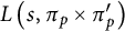 $L\left (s, \pi _{p} \times \pi _{p}^{\prime }\right )$
is defined as a polynomial in
 $p^{-s}$
of degree not exceeding
 $ m m^{ \prime }$
:
 $$ \begin{align} L\left(s, \pi_{p} \times \pi_{p}^{ \prime}\right)^{-1}:=\prod_{j=1}^{m} \prod_{j^{ \prime}=1}^{m^{ \prime}}\left(1-\frac{\alpha_{j, j^{\prime}, \pi \times \pi^{ \prime}}(p)}{p^{s}}\right), \end{align} $$
where
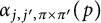 $\alpha _{j, j^{ \prime }, \pi \times \pi ^{ \prime }}(p)$
are suitable complex numbers. Given
 $\theta _{m}$
and
 $\theta _{m^{\prime }}$
as in (3.3), we have the pointwise bound
 $$ \begin{align} \left|\alpha_{j, j^{ \prime}, \pi \times \pi^{ \prime}}(p)\right| \le p^{\theta_{m}+\theta_{m^{ \prime}}} \le p^{1-\frac{1}{m m^{ \prime}}}. \end{align} $$
If
 $p \nmid \mathfrak {q}_{\pi } \mathfrak {q}_{\pi ^{ \prime }}$
, we have
 $$ \begin{align} \bigg\{\alpha_{j, j^{ \prime}, \pi \times \pi^{ \prime}}(p): j \le m, j^{ \prime} \le m^{ \prime}\bigg\}=\bigg\{\alpha_{j, \pi}(p) \overline{\alpha_{j^{\prime }, \pi^{ \prime}}(p)}: j \le m, j^{ \prime} \le m^{\prime }\bigg\}. \end{align} $$
At the archimedean place of
 $\mathbb {Q}$
, there are
 $m m^{\prime }$
complex Langlands parameters
 $\mu _{\pi \times \pi ^{\prime }}\left (j, j^{\prime }\right )$
from which we define the Dirichlet series
 $$ \begin{align*}L_{\infty}\left(s, \pi \times \pi^{\prime}\right):=\pi^{-\frac{m m^{\prime} s}{2}} \prod_{j=1}^{m} \prod_{j^{\prime}=1}^{m^{\prime}} \Gamma\left(\frac{s+\mu_{\pi \times \pi^{\prime}}(j, j^{\prime})}{2}\right). \end{align*} $$
These parameters satisfy the pointwise bound
 $$ \begin{align*}\mathrm{Re}\left(\mu_{\pi \times \pi^{\prime}}\left(j, j^{\prime}\right)\right) \ge-\theta_{m}-\theta_{m^{\prime}}. \end{align*} $$
Let
 $\mathfrak {q}_{\pi \times \pi ^{\prime }}$
denote the conductor of
 $\pi \times \pi ^{\prime }$
. As with
 $L(s, \pi \times \pi ^{\prime })$
, we define the analytic conductor
 $C\left (\pi \times \pi ^{\prime }\right )$
by
 $$ \begin{align} C\left(\pi \times \pi^{\prime}, t\right):=\mathfrak{q}_{\pi \times \pi^{\prime}} \prod_{j=1}^{m} \prod_{j^{\prime}=1}^{m^{\prime}}\left(1+\left|i t+\mu_{\pi \times \pi^{\prime}}\left(j, j^{\prime}\right)\right|\right), \ C\left(\pi \times \pi^{\prime}\right):=C\left(\pi \times \pi^{\prime}, 0\right). \end{align} $$
The combined work of [Reference Bushnell and Henniart4] alongside [Reference Soundararajan and Thorner30, Appendix] shows that
 $$ \begin{align} C\left(\pi \times \pi^{\prime}, t\right) \ll C\left(\pi \times \pi^{\prime}\right)(1+|t|)^{m^{\prime} m}, \quad C\left(\pi \times \pi^{\prime}\right) \le e^{O\left(m^{\prime} m\right)} C(\pi)^{m^{\prime}} C\left(\pi^{\prime}\right)^{m}. \end{align} $$
Let
 $r_{\pi \times \pi ^{\prime }} \in \{0,1\}$
be the order of the pole of
 $L\left (s, \pi \times \pi ^{\prime }\right )$
at
 $s=1$
. We have
 $r_{\pi \times \pi ^{\prime }}=1$
if and only if
 $\pi ^{\prime }=\tilde {\pi }$
. The function
 $\Lambda \left (s, \pi \times \pi ^{\prime }\right )=(s(s-1))^{r_{\pi \times \pi ^{\prime }}} \mathfrak {q}_{\pi \times \pi ^{\prime }}^{s / 2} L\left (s, \pi \right .$
 $\left .\times \pi ^{\prime }\right ) L_{\infty }\left (s, \pi \times \pi ^{\prime }\right )$
is entire of order one. There exists a complex number
 $W\left (\pi \times \pi ^{\prime }\right )$
of modulus one such that
 $$ \begin{align*}\Lambda\left(s, \pi \times \pi^{\prime}\right)=W\left(\pi \times \pi^{\prime}\right) \Lambda\left(1-s, \tilde{\pi} \times \tilde{\pi}^{\prime}\right).\end{align*} $$
Furthermore,
 $L(s, \pi \times \tilde {\pi })$
extends to the complex plane with a simple pole at
 $s=1$
, hence
 $$ \begin{align} \sum_{n\le x} \lambda_{\pi \times \widetilde{\pi}}(n) \sim x \mathrm{Res}_{s=1} L(s, \pi \times \widetilde{\pi}) \ll x, \end{align} $$
as a consequence of a standard Tauberian argument. Taking the logarithmic derivative for
 $L(s, \pi \times \pi ^{\prime })$
, we obtain that, for
 $\mathrm {Re}(s)>1$
,
 $$ \begin{align*}-\frac{L^{\prime}}{L}(s, \pi\times\pi^{\prime})=\sum_{p} \sum_{k=1}^{\infty} \frac{a_{\pi\times\pi^{\prime}} (p^k) \log p}{p^{k s}}=\sum_{n=1}^{\infty} \frac{a_{\pi\times\pi^{\prime}}(n) \Lambda(n)}{n^s},\end{align*} $$
where
 $$ \begin{align*}a_{\pi\times\pi^{\prime}}\left(p^k\right)=\sum_{j=1}^m \sum_{j^{\prime}=1}^{m^{\prime}} \alpha_{j, j^{\prime}, \pi \times \pi^{\prime}}(p)^k. \end{align*} $$
Building upon Shahidi’s non-vanishing result for
 $L(s, \pi \times \tilde {\pi })$
at
 $\mathrm {Re}(s)=1$
(see [Reference Shahidi29]), then
 $$ \begin{align} \sum_{n \le x}\Lambda(n)\left|a_{\pi}(n)\right|{}^{2}\ll\sum_{n \le x} \Lambda(n) a_{\pi \times \widetilde{\pi}}(n) \sim x. \end{align} $$
3.3 Twists
Let
 $\chi $
be a primitive Dirichlet character with conductor q. Fix
 $\pi =\otimes _{p} \pi _{p} \in \mathfrak {E}_{m}$
with
 $m\ge 2$
. By [Reference Cogdell5], the twisted L-function
 $L(s,\pi \otimes \chi )$
equals
 $$ \begin{align*}\sum_{n=1}^{\infty} \frac{\lambda_{\pi \otimes \chi}(n) }{n^s} =\prod_p \prod_{j=1}^m \left(1-\frac{\alpha_{j, \pi \otimes \chi }(p)}{p^s}\right)^{-1}. \end{align*} $$
Furthermore, by (3.11), if
 $p \nmid q$
, then
 $$ \begin{align*}\begin{aligned} \left\{\alpha_{j, \pi\otimes\chi }(p): 1 \le j \le m\right\} =\left\{ \chi(p)\alpha_{j, \pi }(p): 1 \le j \le m\right\}. \end{aligned} \end{align*} $$
Hence, for
 $\mathrm {Re}(s)>1$
, we have
 $$ \begin{align*}\begin{aligned} \sum_{n=1}^{\infty} \frac{\chi(n)\lambda_{\pi }(n) }{n^s} &=\prod_p \prod_{j=1}^m \left(1-\frac{\chi(p)\alpha_{j, \pi }(p)}{p^s}\right)^{-1}=L(s, \pi\otimes\chi ) \prod_{p \mid q} \prod_{j=1}^m\left(1-\frac{\alpha_{j, \pi \otimes \chi}(p)}{p^s}\right). \end{aligned} \end{align*} $$
We use the following zero-free region along with standard contour integration techniques to prove Proposition 2.1.
Lemma 3.2 Let
 $\pi \in \mathfrak {E}_{m}^{b}$
and
 $Q\ge 3$
. There exists a constant
 $c_\pi>0$
, depending effectively on
 $\pi $
, such that for all primitive Dirichlet characters
 $\chi (\bmod \thinspace q)$
with
 $q \le Q$
, with at most one exception, the L-function
 $L(s, \pi \otimes \chi )$
is non-zero in the region
 $$ \begin{align*}\mathrm{Re}(s) \ge 1-\frac{c_\pi}{\log (Q(3+|\mathrm{Im}(s)|))}. \end{align*} $$
If the exceptional character
 $\chi _1$
exists, then
 $\chi _1$
is quadratic.
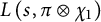 $L\left (s, \pi \otimes \chi _1\right )$
has exactly one zero
 $\beta _1$
in this region, and
 $\beta _1$
is both real and simple. For all
 $\varepsilon _{0}>0$
, there exists an ineffective constant
 $c_\pi (\varepsilon _{0})>0$
depending on
 $\pi $
and
 $\varepsilon _0$
such that
 $\beta _1 \le 1-$
 $c_\pi (\varepsilon _{0}) Q^{-\varepsilon _{0}}$
.
Proof See [Reference Jiang, Lü, Thorner and Wang19, Theorem 4.1].
4 Proof of Propositions 2.1 and 2.2
4.1 Reduction
Define the sum
 $$ \begin{align*}\sum_{n \le x}\Lambda(n)g(n) e(n^{k} \alpha), \end{align*} $$
where
 $ g(n)$
is an arithmetic function. According to the Dirichlet approximation theorem, for any
 $\alpha \in [0,1)$
, there exist integers a and q such that
 $\alpha $
can be expressed as (2.4), where Q is a parameter to be chosen later. Combining (2.4) with partial summation, the above sum is bounded by
 $$ \begin{align} \left(1+\frac{x^{k}}{q Q}\right) \max _{1 \le t \le x}\left|\sum_{n \le t}\Lambda(n) g(n) e\left(\frac{an^{k}}{q}\right)\right|. \end{align} $$
Due to the orthogonality of characters, we find that
 $$ \begin{align} \begin{aligned} \sum_{n \le t}\Lambda(n) g(n) e\left(\frac{a n^{k}}{q}\right) &=\sum_{d \mid q} \sum_{\substack{h=1 \\ (h, q / d)=1}}^{q} e\left(\frac{a d^{k} h^{k}}{q}\right) \sum_{\substack{l \le t / d \\ l \equiv h(\!\!\bmod q / d)}}\Lambda(d l) g(d l) \\ &=\sum_{d \mid q} \sum_{h=1 }^{q/d} e\left(\frac{a d^{k} h^{k}}{q}\right) \sum_{l \le t / d}\Lambda(d l) g(d l)\frac{1}{\varphi(q / d)} \sum_{\substack{\chi(\!\!\bmod q / d)\\ (h, q / d)=1}} \bar{\chi}(h) \chi(l)\\& \ll \sum_{d \mid q} \frac{1}{\varphi(q / d)} \max _{\chi\left(\!\!\bmod q / d\right)}\bigg|\sum_{l \le t / d} \Lambda(d l)g(d l) \chi(l)\bigg| \\ & \quad \times \sum_{\chi\left(\!\!\bmod q / d\right)}\bigg|\sum_{\substack{h=1 \\ (h, q / d)=1}}^{q / d} \bar{\chi}(h) e\left(\frac{ad^k h^k }{q}\right)\bigg|, \end{aligned} \end{align} $$
where
 $\varphi $
is the Euler function. By the Cauchy–Schwarz inequality and Parseval’s identity, the innermost sum over
 $\chi $
is bounded by
 $$ \begin{align} & \varphi\left(q / d\right)^{1/2}\left(\sum_{\chi\left(\!\!\bmod q / d\right)}\bigg|\sum_{\substack{h=1 \\ (h, q / d)=1}}^{q / d} \bar{\chi}(h) e\left(\frac{ad^k h^k }{q}\right)\bigg|^2\right)^{1/2} \nonumber\\ =\ & \varphi\left(q / d\right)^{1/2}\left(\sum_{\substack{h_1=1 \\ \left(h_1, q / d\right)=1}}^{q / d} \sum_{\substack{h_2=1 \\ \left(h_2, q / d\right)=1}}^{q / d} e\left(\frac{ad^k\left(h_1^k-h_2^k\right) }{q}\right) \sum_{\substack{\chi\left(\!\!\bmod q / d\right)}} \bar{\chi}\left(h_1\right) \chi\left(h_2\right)\right)^{1/2} \nonumber\\=\ & \varphi\left(q / d\right)\left(\sum_{\substack{h_1=1 \\ \left(h_1, q / d\right)=1}}^{q / d} \sum_{\substack{h_2=1 \\ h_2 \equiv h_1\left(\!\!\bmod q / d\right)}}^{q / d}e\left(\frac{ad^k\left(h_1^k-h_2^k\right)}{q}\right)\right) ^{1/2}=\varphi\left(q / d\right)^{3/2}. \end{align} $$
Inserting the estimates (4.2) and (4.3) into (4.1), then
 $$ \begin{align} \sum_{n \le x}\Lambda(n) g(n) e\left(n^{k} \alpha\right) \ll \left(1+\frac{x^{k}}{q Q}\right) \max _{1 \le t \le x}\left\{ q^{1 / 2} \sum_{d \mid q} \frac{1}{d^{1 / 2}} \max _{\chi (\!\!\bmod q / d)}\bigg|\sum_{l \le t / d}\Lambda(d l) g(d l) \chi(l)\bigg|\right\}. \end{align} $$
4.2 Proof of Proposition 2.1
It follows from (3.1) and (3.5) that
 $$ \begin{align} \sum_{p\le x}\lambda_{\pi}(p)e(p^{k}\alpha)\log p=\sum_{n \le x}\Lambda(n)a_{\pi}(n) e(n^{k} \alpha)-\sum_{p^{k_1}\le x, k_1\ge 2 } a_{\pi}(p^{k_1})e(p^{k_1}\alpha)\log p. \end{align} $$
Using the Cauchy–Schwarz inequality, (3.14) and (3.15), the left side of the above equation is equal to
 $$ \begin{align} \sum_{n \le x}\Lambda(n)a_{\pi}(n) e(n^{k} \alpha)+O(x^{3/4}). \end{align} $$
Let
 $g(n)=a_{\pi }(n)$
in (4.4). Then the above summation is
 $$ \begin{align} \ll \left(1+\frac{x^{k}}{q Q}\right) \max _{1 \le t \le x}\left\{ q^{1 / 2} \sum_{d \mid q} \frac{1}{d^{1 / 2}} \max _{\chi (\bmod q / d)}\bigg|\sum_{l \le t / d}\Lambda(d l) a_{\pi}(d l) \chi(l)\bigg|\right\}. \end{align} $$
Let
 $l=l_{1} l_{2} $
with
 $l_{1} \mid d^{\infty }$
and
 $\left (l_{2}, l_{1}d\right )=1.$
By the multiplicative property of
 $a_{\pi }(dl)$
, the formula in the brace is
 $$ \begin{align} \ll &q^{1 / 2} \sum_{d \mid q,\ d\neq 1} \frac{1}{d^{1 / 2}} \max _{\chi(\bmod q / d)}\bigg|\sum_{l_{1} \mid d^{\infty},\ l_{1} \le t/d}\Lambda(dl_1) a_{\pi}(dl_{1})\chi(l_{1})\bigg|\nonumber\\ &+q^{1 / 2}\max _{\chi(\bmod q)}\bigg|\sum_{l_{2} \le t} \Lambda(l_{2}) a_{\pi}\left(l_{2}\right) \chi\left(l_{2}\right)\bigg|. \end{align} $$
Due to the property of
 $\Lambda (n)$
and the upper bound of
 $|a_{\pi }(n)|$
, the first item of (4.8) is
 $$ \begin{align} \ll q^{1 / 2}t^{1/2} \sum_{p^{k} \mid q,\ k\ge 1} \frac{1}{p^{k / 2}}\bigg|\sum_{p^{k_1}\le t/p^{k},\ k_1\ge 1}\log p\bigg| \ll (qt)^{1/2}(\log q) \log t. \end{align} $$
If
 $\chi ^{\prime }(\bmod \thinspace q^{\prime })$
is the primitive Dirichlet character that induces
 $\chi (\bmod \thinspace q)$
, then
 $q^{\prime }|q$
. For the second item of (4.8), by (3.3), we get
 $$ \begin{align} \left|\sum_{l_{2} \le t }\Lambda(l_{2}) a_{\pi}\left(l_{2}\right) \chi\left(l_{2}\right)-\sum_{l_{2} \le t } \Lambda(l_{2}) a_{\pi \otimes \chi^{\prime}}(l_{2})\right| \le \sum_{p \mid q} \sum_{p^k \le t, \ k \ge 1}\left|a_\pi\left(p^k\right)\right| \log p \ll_{\varepsilon}t^{\theta_m+\varepsilon}. \end{align} $$
Without loss of generality, assume that
 $\chi ^{\prime }$
is the exceptional character
 $\chi _{1}$
in Lemma 3.2, and let
 $\beta ^{\prime }$
be the corresponding exceptional zero. It follows from (3.13) and (3.12) that the modulus of the conductor of
 $\pi \otimes \chi ^{\prime }$
is smaller than
 $\mathfrak {q}_{\pi }q^{\prime m}$
. We apply [Reference Iwaniec and Kowalski18, Equation (5.52)] to the twisted L-function
 $L(s,\pi \otimes \chi ^{\prime })$
and conclude that
 $$ \begin{align*}\sum_{l_{2} \le t } \Lambda(l_{2}) a_{\pi \otimes \chi^{\prime}}(l_{2})=-\frac{t^{\beta^{\prime}}}{\beta^{\prime}}+O\bigg(\mathfrak{q}_{\pi}^{\frac{1}{2}}q^{\prime\frac{m}{2}}t \exp \left(-\frac{c_\pi}{2} \sqrt{\log t}\right)\bigg). \end{align*} $$
Since Lemma 3.2 gives the bound
 $\beta ^{\prime } \le 1-c_\pi (\varepsilon _0) q^{-\varepsilon _0}$
, where
 $\varepsilon _0>0$
is a fixed constant chosen later, for all
 $q^{\prime }\le q\le (\log t)^{A}$
, we have
 $$ \begin{align*} \sum_{l_{2} \le t } \Lambda(l_{2}) a_{\pi \otimes \chi^{\prime}}(l_{2}) \ll_{\pi} t\exp \left(-c_\pi(\varepsilon_0)(\log t) q^{-\varepsilon_0}\right)+ tq^{\frac{m}{2}} \exp \left(-\frac{c_\pi}{4} \sqrt{\log t}\right). \end{align*} $$
Choose
 $\varepsilon _0=1/(2A)$
. Then inserting (4.7)–(4.10) and the above inequality into (4.6), we get
 $$ \begin{align*}\sum_{p\le x}\lambda_{\pi}(p)e(p^{k}\alpha)\log p \ll_{\pi,A} \bigg(1+\frac{x^{k}}{qQ}\bigg)q^{\frac{m+1}{2}}x \exp \left(-c \sqrt{\log x}\right), \end{align*} $$
where
 $c=\min \left \{\frac {c_\pi }{8},\frac {c_{\pi }(1/(2A))}{2}\right \}$
.
4.3 Proof of Proposition 2.2
Under Hypothesis S, Lemma 3.1 gives that
 $$ \begin{align*}\sum_{l_{2} \le t } \Lambda(l_{2}) a_{\pi \otimes \chi^{\prime}}(l_{2}) \ll mt^{\delta+\varepsilon} (\log t)^{2} \log (\mathfrak{q}_{\pi}q^{m}).\end{align*} $$
Inserting (4.7)–(4.10) and the above inequality into (4.6), we get
 $$ \begin{align*}\sum_{p\le x}\lambda_{\pi}(p)e(p^{k}\alpha)\log p\ll m^{2}\bigg(1+\frac{x^{k}}{qQ}\bigg)q^{\frac{1}{2}}x^{\delta+\varepsilon}(\log x\mathfrak{q}_{\pi})^{3}+x^{3/4}. \end{align*} $$
5 Proof of Theorems 1.1 and 1.2
5.1 Preliminaries and lemmas
The initial step of the Hardy–Littlewood circle method is to divide the unit interval into the major arcs and the minor arcs. The major arcs
 $\mathfrak {M}$
and minor arcs
 $\mathfrak {m}$
are defined as follows:
 $$ \begin{align} \ \ \ \ \ \ \ \ \mathfrak{M}=\bigcup_{q\le P}\bigcup_{1\le a\le q \atop (a, q)=1}\mathfrak{M}(q, a), \ \ \ \mathfrak{M}(q, a)=\Big[\frac{a}{q}-\frac{1}{qQ},\frac{a}{q}+\frac{1}{qQ}\Big], \ \ \ \ \ \mathfrak{m}=\big[1/Q,1+1/Q\big]\setminus \mathfrak{M}, \end{align} $$
where
 $1<2P<Q$
,
 $PQ=N$
, P, Q are parameters to be chosen later. Let
 $$ \begin{align} T_{k,1}(N, \alpha)=\sum_{p_{1} \le N^{1/k}} \lambda_{\pi}(p_{1}) e(p_{1}^{k} \alpha), \quad H_{k, u^{\prime}}(N, \alpha)=\sum_{p_{u^{\prime}} \le N^{1/k}} e(p_{u^{\prime}}^{k} \alpha) \quad (2 \le u^{\prime}\le u). \end{align} $$
Using Parseval’s identity, we write
 $$ \begin{align} \sum_{(p_1,p_2,\dots,p_u)\in\mathcal{J}_{k,u}(N)}\lambda_{\pi}(p_{1}) &=\int_0^1 T_{k,1}(N, \alpha) \prod_{u^{\prime}=2}^{u} H_{k,u^{\prime}}(N, \alpha)e(-N \alpha) \mathrm{d} \alpha\nonumber\\ &=\int_{\mathfrak{M}} T_{k,1}(N, \alpha) \prod_{u^{\prime}=2}^{u} H_{k,u^{\prime}}(N, \alpha)e(-N \alpha) \mathrm{d} \alpha \nonumber\\ &\quad+\int_{\mathfrak{m}} T_{k,1}(N, \alpha) \prod_{u^{\prime}=2}^{u} H_{k,u^{\prime}}(N, \alpha)e(-N \alpha) \mathrm{d} \alpha. \end{align} $$
To control the integral on the minor arcs, we need certain estimates concerning exponential sums over primes.
Lemma 5.1 Suppose that
 $\alpha $
is a real number and there exist integers a and q such that
 $\alpha $
satisfies
 $$ \begin{align} \alpha=\frac{a}{q}+\lambda, \quad 1 \le a \le q, \quad(a, q)=1, \quad|\lambda| \le \frac{1}{q^2}. \end{align} $$
-
(1) For
$k=1$
,
$$ \begin{align*}\sum_{m\le x}\Lambda(m)e(m^{k}\alpha)\ll x (\log x)^3\left(\frac{1}{q}+\frac{1}{x^{2 / 5}}+\frac{q}{x}\right)^{1 / 2}. \end{align*} $$
-
(2) For all
$k \ge 2$
and
$\varepsilon _1>0$
, where
$$ \begin{align*}\sum_{m\le x}\Lambda(m)e(m^{k}\alpha) \ll x^{1+\varepsilon_1}\left(\frac{1}{q}+\frac{1}{x^{1 / 2}}+\frac{q}{x^k}\right)^{1 / K^2}, \end{align*} $$
$K=2^{k-1}$
.


Proof For
 $k=1$
, one can see [Reference Vaughan35]. For
 $k\ge 2$
, one can see [Reference Harman12, Theorem 1].
Sometimes, for
 $k\ge 2$
, it is better to have the factor
 $x^{\varepsilon _1}$
above replaced by some power of
 $\log x$
. This can be done by a simple modification.
Lemma 5.2 Let
 $k \ge 2$
. Suppose that
 $\alpha $
is a real number and there exist integers a and q such that
 $\alpha $
satisfies (5.4). Then
 $$ \begin{align*}\sum_{m\le x}\Lambda(m)e(m^{k}\alpha) \ll x (\log x)^{c^{\prime}}\left(\frac{1}{q}+\frac{1}{x^{1 / 2}}+\frac{q}{x^k}\right)^{1 / (2 K^2)}, \end{align*} $$
where
 $c^{\prime }$
is a positive constant that depends only on k, and K is defined in Lemma 5.1.
Lemma 5.3 Let
 $k\ge 1$
,
 $\gamma _k=1/2+\log k/\log 2$
. Suppose that
 $\alpha $
is a real number and there exist integers a and q such that
 $\alpha $
satisfies (5.4). Then
 $$ \begin{align*}\sum_{m\le x}\Lambda(m)e(m^{k}\alpha)\ll (d(q))^{\gamma_k}\left\{x^{1 / 2} \sqrt{q\left(1+|\lambda| x^k\right)}+x^{4 / 5}+\frac{x}{\sqrt{q\left(1+|\lambda| x^k\right)}}\right\} (\log x)^{c^{\prime\prime}}, \end{align*} $$
where
 $d(n)$
is the divisor function and
 $c^{\prime \prime }$
is an absolute positive constant.
Proof See [Reference Ren28, Theorem 1.1].
5.2 Proof of Theorem 1.1
5.2.1 Major arcs
As for
 $r_{\pi }(N)$
, we use the orthogonality to derive that
 $$ \begin{align} \begin{aligned} \int_0^1\left|H_{1, u^{\prime}}(N, \alpha)\right|{}^2 \mathrm{d}\alpha \le \sum_{p_{u^{\prime}_{1}}\le N}\sum_{p_{u^{\prime}_{2}}\le N} \int_0^1 e((p_{u^{\prime}_{1}}-p_{u^{\prime}_{2}})\alpha)\mathrm{d}\alpha \le \sum_{p\le N}1\ll N/\log N. \end{aligned} \end{align} $$
Let
 $P\le (\log N)^{100B}$
, where P be chosen later. By applying the Cauchy–Schwarz inequality, the above inequality, partial summation and Proposition 2.1,
 $$ \begin{align} \int_{\mathfrak{M}} & T_{1,1}(N, \alpha) H_{1, 2}(N, \alpha)H_{1, 3}(N, \alpha) e(-N \alpha)\mathrm{d} \alpha \nonumber\\ \quad & \ll\left(\max _{\alpha \in\mathfrak{M}}\left|T_{1,1}(N, \alpha)\right|\right)\left\{\int_0^1\left|H_{1,2}(N, \alpha)\right|{}^2 \mathrm{d} \alpha\right\}^{1 / 2} \left\{\int_0^1\left|H_{1,3}(N, \alpha)\right|{}^2 \mathrm{d} \alpha\right\}^{1 / 2}\nonumber \\ & \ll_{\pi,B}P^{\frac{m+1}{2}}N^{2} \exp \left(- c\sqrt{\log N}\right), \end{align} $$
where c is the constant in Proposition 2.1.
Regarding
 $w_{\pi }(N)$
, we apply [Reference Blomer and Granville3, Theorem 3] to give
 $$ \begin{align} \int_0^1\left|H_{2,2}(N, \alpha)H_{2,3}(N, \alpha)\right|{}^2 \mathrm{d} \alpha \le \sum_{p_2^{2}+p_3^{2}=p_2^{\prime2}+p_3^{\prime2}\atop p_2, p_3 ,p_{2}^{\prime },p_3^{\prime}\le N^{1/2} }1\ll N\log N. \end{align} $$
Let
 $P\le (\log N)^{100B}$
, where P be chosen later. It follows from the Cauchy–Schwarz inequality, the above inequality, partial summation and Proposition 2.1 that
 $$ \begin{align} \int_{\mathfrak{M}} T_{2,1}(N, \alpha)&H_{2,2}(N, \alpha)H_{2,3}(N, \alpha)H_{2,4}(N, \alpha)H_{2,5}(N, \alpha)e(-N \alpha)\mathrm{d} \alpha\nonumber\\ \quad \ll&\left(\max _{\alpha \in\mathfrak{M}}\left|T_{2,1}(N, \alpha)\right|\right)\left\{\int_0^1\left|H_{2,2}(N, \alpha)H_{2,3}(N, \alpha)\right|{}^2 \mathrm{d} \alpha\right\}^{1 / 2}\nonumber\\ &\quad \times\left\{\int_0^1\left|H_{2,4}(N, \alpha)H_{2,5}(N, \alpha)\right|{}^2 \mathrm{d} \alpha\right\}^{1 / 2}\nonumber\\ \quad \ll&_{\pi,B}P^{\frac{m+1}{2}}N^{\frac{3}{2}} \exp \left(- \frac{c}{2}\sqrt{\log N}\right), \end{align} $$
where c is the constant in Proposition 2.1.
5.2.2 Minor arcs
By the Polya–Vinogradov inequality and [Reference Iwaniec and Kowalski18, Equation (5.48)],
 $$ \begin{align} \int_0^1\left|T_{k,1}(N, \alpha)\right|{}^2 \mathrm{d} \alpha &\le \sum_{p_{1}\le N^{1/k}}\sum_{p_{2}\le N^{1/k}}\lambda_{\pi}(p_{1}) \bar{\lambda}_{\pi}(p_{2}) \int_0^1 e((p_{1}^{k}-p_{2}^{k})\alpha) \mathrm{d} \alpha\nonumber\\ &\le \sum_{p\le N^{1/k}}|\lambda_{\pi}(p)|^{2 }\ll N^{1/k}m^{2}(\log(N\mathfrak{q}_{\pi}))^{2}. \end{align} $$
Following from the Cauchy–Schwarz inequality, (5.5) and the above inequality, we have
 $$ \begin{align} \int_{\mathfrak{m}} & T_{1,1}(N, \alpha) H_{1, 2}(N, \alpha)H_{1, 3}(N, \alpha) e(-N \alpha)\mathrm{d} \alpha\nonumber \\ \quad & \le\left(\max _{\alpha \in\mathfrak{m}}\left|H_{1,2}(N, \alpha)\right|\right)\left\{\int_0^1\left|T_{1,1}(N, \alpha)\right|{}^2 \mathrm{d} \alpha\right\}^{1 / 2}\left\{\int_0^1\left|H_{1,3}(N, \alpha)\right|{}^2 \mathrm{d} \alpha\right\}^{1 / 2} \nonumber \\ & \ll \left(\max _{\alpha \in\mathfrak{m}}\left|H_{1,2}(N, \alpha)\right|\right)Nm\log(N\mathfrak{q}_{\pi}). \end{align} $$
Using the first inequality in Lemma 5.1 and partial summation, we get
 $$ \begin{align*} \max _{\alpha \in\mathfrak{m}}\left|H_{1,2}(N, \alpha)\right|\ll (Q^{1/2}N^{1/2}+P^{-1/2}N+N^{4/5})(\log N)^{3}. \end{align*} $$
Inserting this bound into (5.10), then
 $$ \begin{align} \begin{aligned} \int_{\mathfrak{m}} & T_{1,1}(N, \alpha) H_{1,2}(N, \alpha) H_{1,3}(N, \alpha) e(-N \alpha) \mathrm{d} \alpha \ll N^{2}m\log(N\mathfrak{q}_{\pi})(P^{-1/2}+N^{-1/5})(\log N)^{3}. \end{aligned} \end{align} $$
For
 $w_{\pi }(N)$
, we obtain that
 $$ \begin{align} \int_0^1\left|T_{2,1}(N, \alpha)H_{2,3}(N, \alpha)\right|{}^2 \mathrm{d} \alpha& \ll \sum_{p_1^{2}+p_3^{2}=p_1^{\prime2}+p_3^{\prime2}\atop p_1, p_3, p_{1}^{\prime }, p_3^{\prime }\le N^{1/2}}|\lambda_{\pi}(p_1)\lambda_{\pi}(p_1^{\prime})|\nonumber\\ &\ll\sum_{p_1\le N^{1/2}}|\lambda_{\pi}(p_{1})|^{2} \sum_{p_1^{\prime}\le N^{1/2}} \sum_{p_1^{2}-p_1^{\prime2}=(p_3^{\prime}+p_3)(p_3^{\prime}-p_3)\atop p_3, p_3^{\prime }\le N^{1/2}}1\nonumber\\ &\ll Nm^{2}\log^{2}(N\mathfrak{q}_{\pi})\log N. \end{align} $$
Treat
 $w_{\pi }(N)$
in the same way as the estimate for
 $r_{\pi }(N)$
, to obtain
 $$ \begin{align} &\int_{\mathfrak{m}} T_{2,1}(N, \alpha)H_{2,2}(N, \alpha)H_{2,3}(N, \alpha)H_{2,4}(N, \alpha)H_{2,5}(N, \alpha)e(-N \alpha)\mathrm{d} \alpha\nonumber\\ & \le\left(\max _{\alpha \in\mathfrak{m}}\left|H_{2,2}(N, \alpha)\right|\right)\left\{\int_0^1\left|T_{2,1}(N, \alpha)H_{2,3}(N, \alpha)\right|{}^2 \mathrm{d} \alpha\right\}^{1 / 2}\nonumber\\&\quad\times\left\{\int_0^1\left|H_{2,4}(N, \alpha)H_{2,5}(N, \alpha)\right|{}^2 \mathrm{d} \alpha\right\}^{1 / 2} \nonumber\\ & \ll \left(\max _{\alpha \in\mathfrak{m}}\left|H_{2,2}(N, \alpha)\right|\right)Nm\log(N\mathfrak{q}_{\pi})\log N. \end{align} $$
In accordance with Lemma 5.2 and by partial summation, we give the following upper bound
 $$ \begin{align*}\max _{\alpha \in\mathfrak{m}}\left|H_{2,2}(N, \alpha)\right|\ll N^{1/2}(\log N)^{c^{\prime}}\left(\frac{1}{P}+\frac{1}{N^{1/4}}+\frac{Q}{N}\right)^{1/8}. \end{align*} $$
Inserting the above estimate into (5.13),
 $$ \begin{align} &\int_{\mathfrak{m}} T_{2,1}(N, \alpha)H_{2,2}(N, \alpha)H_{2,3}(N, \alpha)H_{2,4}(N, \alpha)H_{2,5}(N, \alpha)e(-N \alpha)\mathrm{d} \alpha \nonumber\\ &\ll N^{3/2}m\log(N\mathfrak{q}_{\pi})(\log N)^{c^{\prime}+1}\bigg(P^{-1 / 8} +N^{-1/32}\bigg). \end{align} $$
5.2.3 Choosing parameters
For
 $r_{\pi }(N)$
, we choose
 $P=(\log N)^{2B+8}$
. Then by (5.6), (5.11) and (5.3), we have
 $$ \begin{align*}r_\pi(N)=\sum_{(p_1,p_2,p_3)\in\mathcal{J}_{1,3}(N)} \lambda_{\pi}\left(p_1\right) \ll_{\pi, B} N^{2}(\log N)^{-B}. \end{align*} $$
For
 $w_{\pi }(N)$
, we choose
 $P=(\log N)^{8B+8c^{\prime }+16}$
. It follows from (5.8), (5.14), and (5.3) that
 $$ \begin{align*}w_\pi(N)=\sum_{(p_1,p_2,p_3,p_4,p_5)\in\mathcal{J}_{2,5}(N)} \lambda_{\pi}\left(p_1\right) \ll_{\pi, B} N^{3/2}(\log N)^{-B}.\end{align*} $$
5.3 Proof of Theorem 1.2
We use Proposition 2.2 to improve the upper bounds in (5.6) and (5.8) respectively. Then
 $$ \begin{align} \begin{aligned} \int_{\mathfrak{M}} & T_{1,1}(N, \alpha) H_{1, 2}(N, \alpha)H_{1, 3}(N, \alpha) e(-N \alpha)\mathrm{d} \alpha \ll Pm^2 N^{1+\delta+\varepsilon} (\log ( N\mathfrak{q}_{\pi}))^3+N^{7/4}/\log N \end{aligned} \end{align} $$
and
 $$ \begin{align} \int_{\mathfrak{M}}& T_{2,1}(N, \alpha)H_{2,2}(N, \alpha)H_{2,3}(N, \alpha)H_{2,4}(N, \alpha)H_{2,5}(N, \alpha)e(-N \alpha)\mathrm{d} \alpha\nonumber\\ &\ll Pm^2 N^{1+\delta/2+\varepsilon} (\log ( N\mathfrak{q}_{\pi}))^3\log N+N^{11/8}\log N. \end{align} $$
For
 $r_\pi (N)$
under Hypothesis S, we choose
 $P=N^{\frac {2}{3}(1-\delta )}$
in (5.11) and (5.15) to get
 $$ \begin{align*}r_\pi(N) \ll m^2 N^{5/3+\delta/3+\varepsilon}(\log ( N\mathfrak{q}_{\pi}))^3. \end{align*} $$
For
 $w_\pi (N)$
under Hypothesis S, put
 $P=N^{\frac {1}{3}(1-\delta )}, \ Q=N/P$
and
 $P^{\prime }=N^{1 / 3}, \ Q^{\prime }=N/P^{\prime }$
. On the minor arcs, one notes that each
 $\alpha \in \mathfrak {m}$
can be written as (5.1) with
 $P<q \le Q$
. By Dirichlet’s rational approximation, each
 $\alpha \in \mathfrak {m}$
can also be written as (2.4) with
 $1 \le q \le Q^{\prime }$
and
 $|\lambda | \le 1 / q Q^{\prime }$
. Let
 $\mathfrak {n}$
be the subset of
 $\alpha \in \mathfrak {m}$
such that
 $P^{\prime }<q \le Q^{\prime }$
and
 $|\lambda | \le 1 / qQ^{\prime }$
. We now apply the second inequality of Lemma 5.1 and partial summation to get
 $$ \begin{align} \max _{\alpha \in\mathfrak{n}}\left|H_{2,2}(N, \alpha)\right| \ll N^{1/2+\varepsilon}\left(\frac{1}{P^{\prime}}+\frac{1}{N^{1 / 4}}+\frac{Q^{\prime}}{N}\right)^{1 / 4} \ll N^{7/16+\varepsilon}. \end{align} $$
For
 $\alpha \in \mathfrak {m} \backslash \mathfrak {n}$
, we have
 $$ \begin{align*}P<q \le P^{\prime}, \quad|\lambda| \le \frac{1}{q Q^{\prime}} \end{align*} $$
or
 $$ \begin{align*}q \le P, \quad \frac{1}{q Q}<|\lambda| \le \frac{1}{q Q^{\prime}}. \end{align*} $$
In either case, there holds
 $$ \begin{align*}N^{\frac{1}{6}(1-\delta)}\ll \sqrt{\min \left(P, \frac{N}{Q}\right)} \ll \sqrt{q\left(1+|\lambda| N\right)} \ll \sqrt{P^{\prime}+\frac{N}{Q^{\prime}}} \ll N^{1 /6}. \end{align*} $$
Then Lemma 5.3 gives
 $$ \begin{align} \max _{\alpha \in \mathfrak{m} \backslash \mathfrak{n}}\left|H_{2,2}(N, \alpha)\right| & \ll\left\{N^{1 / 4} \sqrt{q\left(1+|\lambda| N\right)}+N^{2 / 5}+\frac{N^{1/2}}{\sqrt{q\left(1+|\lambda|N\right)}}\right\} d(q)^{2} (\log N)^{c^{\prime\prime}} \nonumber\\ & \ll N^{5 / 12+\varepsilon} +N^{\frac{1}{3}+\frac{\delta}{6}+\varepsilon}. \end{align} $$
Combing (5.17) and (5.18), we derive that
 $$ \begin{align} \max _{\alpha \in \mathfrak{m}}\left|H_{2,2}(N, \alpha)\right| \ll N^{\frac{7}{16}+\varepsilon} +N^{\frac{1}{3}+\frac{\delta}{6}+\varepsilon}. \end{align} $$
It follows from (5.19), (5.13), (5.16), and (5.3) that
 $$ \begin{align*}w_{\pi}(N)\ll m^{2}(N^{\frac{23}{16}+\varepsilon}+N^{\frac{4}{3}+\frac{\delta}{6}+\varepsilon})(\log ( N\mathfrak{q}_{\pi}))^3. \end{align*} $$
This finishes the proof of Theorem 1.2.
Remark For
 $w_\pi (N)$
under Hypothesis S, if we refrain from subdividing the minor arcs further and instead individually apply Lemma 5.1 or Lemma 5.3, we obtain the following two results.
-
(1) Using the second inequality of Lemma 5.1 and choosing
$P=N^{\frac 25(1-\delta )}$
, we have Inserting this into (5.13) and combing (5.16), we obtain
$$ \begin{align*} \max _{\alpha \in\mathfrak{m}}\left|H_{2,2}(N, \alpha)\right| \ll N^{1/2+\varepsilon}\left(\frac{1}{P}+\frac{1}{N^{1 / 4}}\right)^{1 / 4} \ll N^{2/5+\delta/10+\varepsilon}. \end{align*} $$
$$ \begin{align*}w_{\pi}(N)\ll m^{2}N^{\frac{7}{5}+\frac{\delta}{10}+\varepsilon}(\log ( N\mathfrak{q}_{\pi}))^3. \end{align*} $$
-
(2) Similarly, using Lemma 5.3 and choosing
$P=N^{1/2-\delta /3}$
, we have Then
$$ \begin{align*} \max _{\alpha \in\mathfrak{m}}\left|H_{2,2}(N, \alpha)\right| \ll N^{1/2+\varepsilon}\left(N^{1/4}P^{-1/2}+N^{-1 / 10}\right) \ll N^{1/2+\delta/6+\varepsilon}. \end{align*} $$
$$ \begin{align*}w_{\pi}(N)\ll m^{2}N^{3/2+\delta/6+\varepsilon}(\log ( N\mathfrak{q}_{\pi}))^3. \end{align*} $$





By directly comparing the aforementioned two results, it becomes evident that
 $N^{\frac {7}{5}+\frac {\delta }{10}+\varepsilon }$
and
 $N^{3/2+\delta /6+\varepsilon }$
are larger than
 $(N^{\frac {23}{16}+\varepsilon }+N^{\frac {4}{3}+\frac {\delta }{6}+\varepsilon })$
. Hence, the rationale behind further subdividing the minor arcs is stronger.
6 Preliminaries and proof of Theorem 1.4
6.1 The modular L-functions
Fix a non-CM form
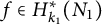 $f\in H_{k_{1}}^*(N_1)$
. Let
 $$ \begin{align*}f(z)=\sum_{n=1}^{\infty} \lambda_f(n) n^{(k_{1}-1) / 2} e(n z) \end{align*} $$
be its normalized Fourier expansion at the cusp
 $\infty $
. For each prime p, let
 $\theta _{p} \in [0, \pi ]$
be the unique angle such that
 $\lambda _{f}(p)=2 \cos \theta _{p}$
. The modular L-function
 $L(s, f)$
associated with f has the Euler product representation
 $$ \begin{align*}L(s, f)=\sum_{n=1}^{\infty} \frac{\lambda_{f}(n)}{n^{s}}=\prod_{p}\left(1-\frac{\lambda_{f}(p)}{p^{s}}+\frac{\chi_{0}(p)}{p^{2 s}}\right)^{-1}, \quad \mathrm{Re}(s)>1, \end{align*} $$
where
 $\chi _{0}$
is the trivial Dirichlet character modulo
 $N_1$
. Let’s rewrite the Euler product as
 $$ \begin{align*}L(s, f)=\prod_{p \mid q}\left(1-\frac{\left(-\lambda_{p} p^{-\frac{1}{2}}\right)}{p^{s}}\right) \prod_{p \nmid q} \prod_{j=0}^{1}\left(1-\frac{e^{i(2 j-1) \theta_{p}}}{p^{s}}\right)^{-1}, \quad \mathrm{Re}(s)>1, \end{align*} $$
where
 $\lambda _{p} \in \{-1,1\}$
is the eigenvalue of the Atkin–Lehner operator
 $|_{k_1} W\left (Q_{p}\right )$
. According to Deligne [Reference Deligne7], for any prime p, there are two numbers
 $\alpha _{f}(p)$
and
 $\beta _{f}(p)$
such that
 $$ \begin{align} \alpha_{f}(p)=e^{i \theta_{p}},\quad \beta_{f}(p)=e^{-i \theta_{p}} \end{align} $$
and
 $$ \begin{align*}\lambda_{f}(p)=\alpha_{f}(p)+\beta_{f}(p) \end{align*} $$
with
 $\theta _{p} \in [0, \pi ]$
. Deligne proved the Ramanujan–Petersson conjecture, which states that
 $$ \begin{align*}\left|\lambda_{f}(n)\right| \le d(n). \end{align*} $$
For each
 $j \ge 1$
and
 $\mathrm {Re}(s)>1$
, the jth symmetric power L-function attached to f is defined by
 $$ \begin{align} L\left(s, \mathrm{sym}^{j} f\right)=\sum_{n=1}^{\infty} \frac{\lambda_{\mathrm{sym}^{j} f}(n)}{n^{s}}=\prod_{p \mid q} \prod_{m=0}^{j}\left(1-\frac{\alpha_{ \mathrm{sym}^{j}f,m }(p)}{p^{s}}\right)^{-1} \prod_{p \nmid q} \prod_{m=0}^{j}\left(1-\frac{e^{i(2 m-j) \theta_{p}}}{p^{s}}\right)^{-1}. \end{align} $$
The values
 $\alpha _{ \mathrm {sym}^{j}f,m }(p)$
can be determined by using [Reference Soundararajan and Thorner30, Appendix] and [Reference David, Gafni, Malik, Prabhu and Turnage-Butterbaugh6, Appendix]. Note that
 $L\left (s,\mathrm {sym}^{1} f\right )=L(s, f)$
and
 $L\left (s,\mathrm {sym}^{0} f\right )=\zeta (s)$
. It is well known that
 $\lambda _{\mathrm {sym}^{j} f}(n)$
is a real multiplicative function. Via (6.2), one easily verify that
 $$ \begin{align} \lambda_{\mathrm{sym}^{j} f}(p)=\frac{\sin(n+1)\theta_p}{\sin \theta_p}=U_{j}\left(\cos \theta_{p}\right), \quad p \nmid N_1. \end{align} $$
Let
 $\Gamma _{\mathbb {R}}(s):=\pi ^{-s/2}\Gamma (s/2)$
and
 $\Gamma _{\mathbb {C}}(s)=\Gamma _{\mathbb {R}}(s) \Gamma _{\mathbb {R}}(s+1)$
. With these definitions, we obtain that
 $$ \begin{align} L\left(s,\left(\mathrm{sym}^j f\right)_{\infty}\right)= \begin{cases}q_{\mathrm{sym}^j f} \prod_{m=1}^{(j+1) / 2} \Gamma_{\mathbb{C}}\left(s+\left(m-\frac{1}{2}\right)(k-1)\right), & \text { if } j \text { is odd}, \\ q_{\mathrm{sym}^j f} \Gamma_{\mathbb{R}}(s+r) \prod_{m=1}^{j / 2} \Gamma_{\mathbb{C}}(s+m(k-1)), & \text { if } j \text { is even},\end{cases} \end{align} $$
where
 $q_{\mathrm {sym}^{j} f}$
is a suitable integer, and
 $r=0$
if
 $j \equiv 0\ (\!\bmod \ 4)$
, and
 $r=1$
if
 $j \equiv 2\ (\!\bmod \ 4)$
. Let
 $C(\mathrm {sym}^{j}f)$
be the analytic conductor of
 $L(s, \mathrm {sym}^{j}f)$
. For any primitive Dirichlet character
 $\chi $
, we give a proof that the twist L-function
 $L(s, \mathrm {sym}^{j}f\otimes \chi )$
has no Landau–Siegel zeros.
Lemma 6.1 Let Q be a large positive number and
 $\chi $
be a primitive Dirichlet character modulo q with
 $q\le Q$
. Define
 $$\begin{align*}y_{f} = \begin{cases} 0 & \text{if } f \text{ has squarefree level or } f \text{ corresponds}\\ &\text{with a non-CM elliptic curve over } \mathbb{Q}, \\ 2 & \text{otherwise}. \end{cases} \end{align*}$$
There exists a constant
 $c_{9}>0$
such that if
 $n \ge 1$
, then
 $L\left (s, \operatorname {sym}^n f \otimes \chi \right ) \neq 0$
for
 $$ \begin{align*} \mathrm{Re}(s) \ge 1-\frac{c_{9}}{n^{2+y_{f}} \log (nk_1N_1Q (3+|\operatorname{Im}(s)|))}. \end{align*} $$
Proof The proof can be found in [Reference Thorner34, Corollary 1.3].
6.2 The Sato–Tate conjecture
Serre’s modular version of the Sato–Tate conjecture posits that if f is non-CM, then the sequence
 $\left \{\theta _{p}\right \}$
is uniformly distributed in the interval
 $[0, \pi ]$
with respect to the measure
 $\mathrm {d} \mu _{S T}:=(2 / \pi ) \sin ^{2} \theta \mathrm {d} \theta $
. More explicitly, let
 $I_{0}$
be a subinterval of
 $[-2,2]$
, and for a positive real number x, define the set
 $$ \begin{align*} N_{I_{0}}(f, x):=\#\left\{p \le x: \mathrm{gcd}(p, N_1)=1, \lambda_f(p) \in I_{0}\right\}. \end{align*} $$
The Sato–Tate conjecture states that for a fixed non-CM form
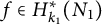 $f \in H_{k_{1}}^*(N_1)$
, we have
 $$ \begin{align*} \lim _{x \rightarrow \infty} \frac{N_{I_{0}}(f, x)}{\pi(x)}=\int_{I_{0}} \mu_{\infty}(t) \mathrm{d} t, \end{align*} $$
where
 $$ \begin{align*}\mu_{\infty}(t):= \begin{cases} \frac{1}{\pi} \sqrt{1-\frac{t^2}{4}}, & \text { if } t \in[-2,2], \\ 0, & \text { otherwise. } \end{cases} \end{align*} $$
If
 $\chi _I$
is the indicator function of the interval
 $I=[\alpha , \beta ]\subseteq [0,\pi ]$
, then
 $$ \begin{align*}\sum_{\substack{p \le x \\ \lambda_{f}(p) \in [2\cos\beta, 2\cos\alpha]}}1=\sum_{p \le x} \chi_I\left(\theta_p\right). \end{align*} $$
Thorner [Reference Thorner32] approximate
 $\chi _I$
with a differentiable function using the following construction formula in [Reference Vinogradov37].
Lemma 6.2 Let R be a positive integer, and let
 $a, b, \delta ^{\prime } \in \mathbb {R}$
satisfy
 $$ \begin{align*}0<\delta^{\prime}<1 / 2, \quad \delta^{\prime} \le b-a \le 1- \delta^{\prime}. \end{align*} $$
Then there exists an even periodic function
 $g(y)$
with period 1 satisfying
-
(1)
$g(y)=1$
when
$y \in \left [a+\frac { \delta ^{\prime }}{2} , b-\frac { \delta ^{\prime }}{2}\right ]$
, -
(2)
$g(y)=0$
when
$y \in \left [b+\frac { \delta ^{\prime }}{2}, 1+a-\frac { \delta ^{\prime }}{2}\right ]$
, -
(3)
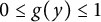
$0 \le g(y)\le 1$
when y is in the rest of the interval
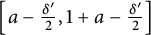
$\left [a-\frac { \delta ^{\prime }}{2} , 1+a-\frac { \delta ^{\prime }}{2} \right ]$
, and
$g(y)$
has the Fourier expansion where for all
$$ \begin{align*}g(y)=b-a+\sum_{n=1}^{\infty}\left(a_n \cos (2 \pi n y)+b_n \sin (2 \pi n y)\right), \end{align*} $$
$n \ge 1$
,
$$ \begin{align*}\left|a_n\right|,\left|b_n\right| \le \min \left\{2(b-a), \frac{2}{n \pi}, \frac{2}{n \pi}\left(\frac{R}{\pi n \delta^{\prime}}\right)^R\right\}. \end{align*} $$

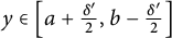




6.3 Proof of Theorem 1.4
If
 $\chi _I$
is the indicator function of the interval
 $I=[\alpha , \beta ]\subseteq [0,\pi ]$
, then
 $$ \begin{align*}\# \mathcal{J}_{1,3,f, I}(N)=\sum_{\substack{(p_1,p_2,p_3)\in\mathcal{J}_{1,3}(N) \\ \lambda_{f}(p_1) \in [2\cos\beta, 2\cos\alpha]}} 1=\sum_{(p_1,p_2,p_3)\in\mathcal{J}_{1,3}(N)} \chi_I\left(\theta_{p_1}\right). \end{align*} $$
Let
 $g(\theta _{p_1})$
be defined as in Lemma 6.2 with
 $a=\frac {\alpha }{2 \pi }-\frac {\delta ^{\prime }}{2}$
and
 $b=\frac {\beta }{2 \pi }+\frac {\delta ^{\prime }}{2}$
. Thorner [Reference Thorner32] constructed
 $g^{+}(\theta _{p_1}; I, \delta ^{\prime })=g\Big (\frac {\theta _{p_1}}{2 \pi }\Big )+g\Big (-\frac {\theta _{p_1}}{2 \pi }\Big )$
as a pointwise upper bound for
 $\chi _I(\theta _{p_1})$
. By repeating this construction with
 $a=\frac {\alpha }{2 \pi }+\frac {\delta ^{\prime }}{2}$
, and
 $b=\frac {\beta }{2 \pi }-\frac {\delta ^{\prime }}{2}$
, we can get a lower bound
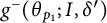 $g^{-}(\theta _{p_1}; I, \delta ^{\prime })$
for
 $\chi _I(\theta _{p_1})$
. Thus, according to Lemma 6.2, we can express
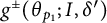 $g^{\pm }(\theta _{p_1}; I, \delta ^{\prime })$
in terms of the basis of Chebyshev polynomials of the second kind
 $\{U_n(\cos (\theta _{p_1})) \}_{n=0}^{\infty }$
as follows:
 $$ \begin{align} g^{\pm}(\theta_{p_1}; I, \delta^{\prime})=a_0^{\pm}(I, \delta^{\prime})-a_2^{\pm}(I, \delta^{\prime})+\sum_{n=1}^{\infty}\left(a_n^{\pm}(I, \delta^{\prime})-a_{n+2}^{\pm}(I, \delta^{\prime})\right) U_n(\cos (\theta_{p_1})), \end{align} $$
where
 $a_n^{\pm }(I, \delta ^{\prime })$
represents the nth Fourier coefficient in the cosine expansion of
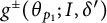 $g^{\pm }(\theta _{p_1}; I, \delta ^{\prime })$
. Furthermore, we derive
 $$ \begin{align} \begin{aligned} \left|a_0^{\pm}(I, \delta^{\prime})-a_2^{\pm}(I, \delta^{\prime})-\mu_{S T}(I)\right| & \ll \delta^{\prime} , \end{aligned} \end{align} $$
and for
 $n\ge 1$
,
 $$ \begin{align} \left|a_n^{\pm}(I, \delta^{\prime})\right|,\left|a_{n+2}^{\pm}(I, \delta^{\prime})\right| \le \min \left\{2(b-a), \frac{2}{n \pi}, \frac{2}{n \pi}\left(\frac{R}{\pi n \delta^{\prime}}\right)^R\right\}.\end{align} $$
Following the method in [Reference Thorner31], when summing
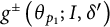 $g^{\pm }\left (\theta _{p_1}; I, \delta ^{\prime }\right )$
over
 $\mathcal {J}_{1, 3}(N)$
, we can interchange the order of summation by choosing R to ensure absolute convergence. Thus by (6.5), we obtain the following expression:
 $$ \begin{align*}\begin{aligned} \sum_{(p_1,p_2,p_3)\in\mathcal{J}_{1,3}(N)} g^{\pm}(\theta_{p_1}; I, \delta^{\prime}) &=\sum_{(p_1,p_2,p_3)\in\mathcal{J}_{1,3}(N)}(a_0^{\pm}(I, \delta^{\prime})-a_2^{\pm}(I, \delta^{\prime}))\nonumber\\ &\quad+\sum_{(p_1,p_2,p_3)\in\mathcal{J}_{1,3}(N)}\bigg(\sum_{n=1}^{\infty}\left(a_n^{\pm}(I, \delta^{\prime})-a_{n+2}^{\pm}(I, \delta^{\prime})\right) U_n(\cos (\theta_{p_1}))\bigg)\nonumber\\ &=(a_0^{\pm}(I, \delta^{\prime})-a_2^{\pm}(I, \delta^{\prime}))\sum_{(p_1,p_2,p_3)\in\mathcal{J}_{1,3}(N)}1\nonumber\\ &\quad+\sum_{n=1}^{\infty}\left(a_n^{\pm}(I, \delta^{\prime})-a_{n+2}^{\pm}(I, \delta^{\prime})\right)\sum_{(p_1,p_2,p_3)\in\mathcal{J}_{1,3}(N)}U_n(\cos (\theta_{p_1})).\end{aligned} \end{align*} $$
It follows from (6.6), (6.7), and (6.3) and the above equation that
 $$ \begin{align} \begin{aligned} \sum_{(p_1,p_2,p_3) \in\mathcal{J}_{1,3}(N)} \chi_I\left(\theta_{p_1}\right) =(\mu_{\mathrm{ST}}(I)+O(\delta^{\prime}))\bigg(\sum_{(p_1,p_2,p_3)\in\mathcal{J}_{1,3}(N)} 1\bigg)+O(A), \end{aligned} \end{align} $$
where
 $$ \begin{align} A=\sum_{n=\delta^{\prime-1}}^{\infty}\frac{4}{n \pi}\left(\frac{R}{\pi n \delta^{\prime}}\right)^R \sum_{(p_1,p_2,p_3)\in\mathcal{J}_{1,3}(N)}\lambda_{\mathrm{sym}^{n}f}(p_1)+\sum_{n=1}^{\delta^{^\prime-1}} \frac{2}{n\pi}\sum_{(p_1,p_2,p_3)\in\mathcal{J}_{1,3}(N)}\lambda_{\mathrm{sym}^{n}f}(p_1). \end{align} $$
Let
 $\pi _{f} \in \mathfrak {E}_{2}$
correspond to f. It is known from [Reference Newton and Thorne25] and [Reference Newton and Thorne26] that
 $\mathrm {sym}^{j} f$
corresponds to
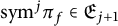 $\mathrm {sym}^{j}\pi _{f} \in \mathfrak {E}_{j+1}$
. Utilizing the method outlined in the proof of Theorem 1.2, (3.7) with the zero-free region in Lemma 6.1, and [Reference Thorner33, Equation (6.5)], if the level of f is squarefree, we derive the inequality
 $$ \begin{align*}\sum_{(p_1,p_2,p_3)\in\mathcal{J}_{1,3}(N)} \lambda_{\mathrm{sym}^{n}f}(p_1)\ll (n+1) N^{2} \exp\bigg(-\frac{c_{9}\log N}{n^2 \log (nk_1N_1\log N )} \bigg). \end{align*} $$
Based on Lemma 6.2, we choose
 $\delta ^{\prime -1}=(\log N)^{1/2} / \log (k_1 N_1 \log N)$
, and
 $R=2$
in (6.9), then
 $$ \begin{align*}A\ll \frac{N^{2} (\log N)^{1/2}}{\log (k_1 N_1 \log N)}\exp\bigg(-\frac{c_{9}\log^{2} (k_1 N_1 \log N)}{ \log ( k_1N_1 \log^{2} N )} \bigg). \end{align*} $$
Inserting this upper bound of A into (6.8), we have
 $$ \begin{align*}\sum_{(p_1,p_2,p_3)\in\mathcal{J}_{1,3}(N)} \chi_I\left(\theta_{p_1}\right) =\mu_{\mathrm{ST}}(I)\left(\# \mathcal{J}_{1,3}(N)\right)+O\left(\frac{\log (k_1 N_1 \log N)}{ (\log N)^{1/2} }\left(\# \mathcal{J}_{1,3}(N)\right)\right). \end{align*} $$
Similar to the discussion above, if the level of f is not squarefree, we choose
 ${\delta ^{\prime -1}=(\log N)^{1/4} / \log (k_1 N_1 \log N)}$
and
 $R=2$
in (6.9) to obtain
 $$ \begin{align*}\sum_{(p_1,p_2,p_3)\in\mathcal{J}_{1,3}(N)} \chi_I\left(\theta_{p_1}\right) =\mu_{\mathrm{ST}}(I)\left(\# \mathcal{J}_{1,3}(N)\right)+O\left(\frac{\log (k_1 N_1 \log N)}{ (\log N)^{1/4} }\left(\# \mathcal{J}_{1,3}(N)\right)\right). \end{align*} $$
Under Hypothesis S, and using the method outlined in the proof of Theorem 1.2, (3.7), and [Reference Thorner33, Equation (6.5)], we derive the inequality:
 $$ \begin{align*}\sum_{(p_1,p_2,p_3)\in\mathcal{J}_{1,3}(N)} \lambda_{\mathrm{sym}^{n}f}(p_1)\ll (n+1) N^{5/3+\delta/3}(\log N)^3\log (k_1N_1n). \end{align*} $$
In (6.9), we choose
 $\delta ^{\prime }=RN^{\delta /6-1/6}\log ( k_1N_1N)$
and
 $R=2$
based on Lemma 6.2, then
 $$ \begin{align*}A \ll N^{11/6+\delta/6}(\log N)^{3}. \end{align*} $$
Substituting this upper bound of A into (6.8), we have
 $$ \begin{align*}\sum_{(p_1,p_2,p_3)\in\mathcal{J}_{1,3}(N)} \chi_I\left(\theta_{p_1}\right) =\mu_{\mathrm{ST}}(I)\left(\# \mathcal{J}_{1,3}(N)\right)+O(N^{11/6+\delta/6}(\log N)^{3}). \end{align*} $$
7 Appendix
In this section, for a better understanding of the results in Theorem 1.3, we provide asymptotic formulas for the ternary Goldbach conjecture, as well as an asymptotic formula for the number of the sums of five square primes.
Lemma 7.1 For a large integer N, we have
-
(1)
where
$$ \begin{align*}\# \mathcal{J}_{1,3}(N) =\mathfrak{G}_{1,3}(N)\frac{N^2}{2(\log N)^{3}}+O\left(\frac{N^{2}\log \log N}{(\log N)^{4}}\right), \end{align*} $$
$\mathfrak {G}_{1,3}(N)$
is the singular series defined in (1.1) and satisfies
$\mathfrak {G}_{1,3}(N)\ge 1/2$
for odd N.
-
(2)
where
$$ \begin{align*} \# \mathcal{J}_{2,5}(N)= \mathfrak{G}_{2,5}(N)\frac{\pi^2N^{3/2}}{24(\log N)^{5}}+O\left(\frac{N^{3/2}\log \log N}{(\log N)^{6}}\right), \end{align*} $$
$\mathfrak {G}_{2,5}(N)$
is absolutely convergent and satisfies
$\mathfrak {G}_{2,5}(N)\gg 1$
for
$N\equiv 5\ (\mathrm {mod}\ 24)$
.







Proof One can see the detail proof in [Reference Hua16, Theorem 11]. Here we take the first equation as an example to illustrate the main ideas. By the Hardy–Littlewood circle method, we consider
 $$ \begin{align*} \# \mathcal{J}_{1,3}(N) &=\left\{\int_{\mathfrak{M}}+\int_{\mathfrak{m}}\right\}H_{1, 1}(N, \alpha) H_{1, 2}(N, \alpha)H_{1, 3}(N, \alpha)e(-N \alpha) \mathrm{d} \alpha, \end{align*} $$
where
 $\mathfrak {M}$
and
 $\mathfrak {m}$
are defined in (5.1). For the integral on the minor arcs, we follow a similar approach as in (5.10), but replace
 $T_{1, 1}(N, \alpha )$
with
 $H_{1, 1}(N, \alpha )$
. Regarding the major arcs, due to the sparsity of prime numbers, we seek an equation that establishes a connection between prime numbers and integers to derive an asymptotic formula. Consider
 $$ \begin{align*} H_{1, i}(N, \alpha)&= \sum_{\substack{h=1 \\ (h, q)=1}}^q e\left(\frac{a h}{q}\right) \sum_{\substack{\sqrt{N}<p \le N \\ p\equiv h~(\!\!\bmod q)}} e\left(p \lambda\right)+O(\sqrt{N}) \\ &= \mu(q) \int_{\sqrt{N}}^{N}e(u\lambda)\mathrm{d}\sum_{p\le u, ~p\equiv h~(\mathrm{mod}~q)}1+O(\sqrt{N}). \end{align*} $$
When
 $q\le \log ^{A}u$
, by Siegel–Walfisz theorem, we have
 $$ \begin{align*}\sum_{p\le u, ~p\equiv h~(\mathrm{mod}~q)}1=\frac{\mathrm{Li}(u)}{\varphi(q)}+O(ue^{-c\sqrt{\log u}}), \quad\quad \mathrm{Li}(u)=\int_{2}^{u}\frac{\mathrm{d} t}{\log t}. \end{align*} $$
Moreover, under the generalized Riemann hypothesis (GRH in brief), the error term can be improved to
 $$ \begin{align*}O(u^{1/2}\log^2 u). \end{align*} $$
By substituting either of the above equations into the major arcs, and using the properties of characteristic functions with the integral in [Reference Hua16, Theorem 11], we get the first equation.
The proof shows the error term in the asymptotic formula cannot be improved under GRH, which is different from Theorem 1.2. One needs to explore other methods for improving the error term.
Acknowledgements
The authors are deeply grateful to Binyong Sun for helpful discussions. They also thank Jesse Thorner for his valuable comments and the referee for the critical historical comments.
Conflict of interest
On behalf of all authors, the corresponding author states that there is no conflict of interest.
Data availability statement
Data sharing not applicable to this article as no datasets were generated or analyzed during the current study.



