3.2.1 Pressure

The distribution of pressure over the model surface is shown in figure 7. The tick surface shown in figures is not scaled with the right aspect ratio in the $y$ coordinate but included for representation purposes only. For correct surface dimensions, refer to figure 2. Both models exhibit similar features such as a pressure plateau and a dip from the peak before attaining a constant value further downstream. The establishment of a pressure plateau after separation is a characteristic of well-separated flows. The dip from the peak exemplifies an Edney type VI interaction at the triple point as explained in § 2.2. Such a dip in surface parameters as a result of shock interactions is a typical characteristic of hypersonic flows (Holden Reference Holden1971). Separation and reattachment locations are marked in figure 7 but physical aspects underlying these particular locations are described in § 3.2.3.

Figure 7.

Normalised pressure distribution along the wall.

A noticeable feature is that the plateau pressure is higher for the blunt leading edge. This indicates stronger vorticity gradients within the recirculation region. Another vorticity-generated phenomenon is the slight dip in pressure just after the plateau region and before rising towards the reattachment. This is noticeable in both cases but occurs slightly earlier for the sharp case (at $x/x_{c}=1.32$ ) relative to the blunt model (at $x/x_{c}=1.40$ ). A possible reason for this dip is the presence of a Moffat eddy at the corner (Moffat Reference Moffat1964; Korolev, Gajjar & Ruban Reference Korolev, Gajjar and Ruban2002). Over the compression surface, the high-speed reverse flow of the primary recirculation streamlines close to the surface and extending from the reattachment towards the corner generates significant shear. This results in a continual drop in reverse-flow kinetic energy as the streamlines move towards the corner. If the shear is large, the available kinetic energy would not be able to overcome this and reach the corner. Dissipative effects then result in breaking down the primary recirculation region into a primary vortex and a secondary vortex (Moffat eddy) at the corner. Thus, the formation and evolution of the secondary corner vortex occur through vorticity-enhanced energy transfer from the primary recirculation region. This feeding of energy into the secondary vortex occurs at its downstream end. Thus, within the secondary vortex region, the local velocity at the downstream end tends to be higher and causes a dip in pressure. A shallower and spatially delayed dip for the blunt case, therefore, indicates a relatively enlarged secondary structure (see figure 14). The aforementioned rationale will be explored and elucidated further in § 3.3.2 while discussing the vorticity distribution over the flow domain.

The enhanced vorticity and the resulting enlargement of secondary structures within the primary recirculation region displace the reattachment location downstream and lead to an overall increase in the separation region size. This is illustrated in figure 7, in which the reattachment for the blunt model is further downstream relative to the sharp case. When the reattachment is displaced downstream, the bending of the shear layer parallel to the compression surface occurs gradually and results in a shallower angle between the surface and stacks of compression waves that coalesce to form the recompression shock. The strength of the recompression shock is barely affected, as evidenced by similar peak magnitudes, but the region of compression waves gets wider and results in a relatively smoother and extended peak region.

The inset in figure 7 depicts the region close to the leading edge within a distance of $x/x_{c}=0.1$ . The non-dimensional distance to separation from the leading edge is increased by 40 % for the blunt case relative to a sharp leading edge. This is consistent with the beginning of interaction at $x/x_{c}=0.025$ and 0.032 for sharp and blunt cases, respectively. It is interesting to note that, regardless of the curvature induced by the bluntness and the inherent local flow acceleration, the pressure is higher for the blunt leading edge. This indicates that the flow in the vicinity of the leading edge is strongly influenced by viscous interactions between the leading-edge shock and the boundary layer rather than effects of a finite bluntness. A characteristic parameter determining the flow physics over surfaces with a finite leading-edge radius is the combined bluntness–viscous interaction parameter $\unicode[STIX]{x1D6FD}$ , which is given as (Cheng et al. Reference Cheng, Hall, Golian and Hertzberg1961; Holden Reference Holden1971; Mallinson, Gai & Mudford Reference Mallinson, Gai and Mudford1996)

(3.2) $$\begin{eqnarray}\unicode[STIX]{x1D6FD}=\frac{\overline{\unicode[STIX]{x1D712}}_{\unicode[STIX]{x1D700}}}{\unicode[STIX]{x1D705}_{\unicode[STIX]{x1D700}}^{2/3}},\end{eqnarray}$$

where

(3.3a ) $$\begin{eqnarray}\displaystyle & \displaystyle \overline{\unicode[STIX]{x1D712}}_{\unicode[STIX]{x1D700}}=\unicode[STIX]{x1D700}\left(0.664+1.73\frac{h_{w}}{h_{0}}\right)M_{e}^{3}\sqrt{\frac{C^{\ast }}{Re_{s_{p}}}}, & \displaystyle\end{eqnarray}$$

(3.3b ) $$\begin{eqnarray}\displaystyle & \displaystyle \unicode[STIX]{x1D705}_{\unicode[STIX]{x1D700}}=\unicode[STIX]{x1D700}M_{e}^{3}\frac{C_{D}}{s_{p}/d}, & \displaystyle\end{eqnarray}$$

(3.3c ) $$\begin{eqnarray}\displaystyle & \displaystyle C^{\ast }=\frac{\unicode[STIX]{x1D707}^{\ast }T_{e}}{\unicode[STIX]{x1D707}_{e}T^{\ast }}, & \displaystyle\end{eqnarray}$$

$h$

$M$

$\unicode[STIX]{x1D707}$

$T$

$w$

$0$

$e$

$\overline{\unicode[STIX]{x1D712}}_{\unicode[STIX]{x1D700}}$

$\unicode[STIX]{x1D705}_{\unicode[STIX]{x1D700}}$

$C^{\ast }$

$T^{\ast }$

$Re$

$s_{p}$

$C_{D}$

$d$

$\unicode[STIX]{x1D6FD}\leqslant 0.1$

$\unicode[STIX]{x1D6FD}>0.1$

$C_{D}$

$\unicode[STIX]{x1D6FD}$

Even though the flow is dominated by viscous effects at the leading edge, the introduction of a finite bluntness plays a role in shaping the viscous interactions that determine the boundary layer growth and its separation. This is the reason behind the differences in the behaviour close to the leading edge between the two models. Compared to a sharp case, the $20~\unicode[STIX]{x03BC}\text{m}$ leading-edge shock is stronger, and this generates a stronger entropy gradient in the shock layer. However, the strongest entropy changes in the surface-normal direction are not large enough to completely submerge the boundary layer, contrary to bluntness-dominated flows such as behind a detached bow shock that typically sits in front of significantly blunted leading edges. Since the leading-edge shock attenuates rapidly away from the surface for the bluntness considered here, the stronger entropy region would then be confined much closer to the surface. This causes the initial part of the streamwise boundary layer growth in the vicinity of the merged layer affected by the entropy gradient. The extent of entropy outside the boundary layer edge, within this region of its initial growth stage, facilitates a continuous energy transfer from the outer inviscid flow to lower layers of the boundary layer through viscous interactions. This transfer energises the lower part and, thereby, increases the resistance to adverse pressure gradients that initiate separation and results in a delayed separation for the blunt case, as shown in figure 7. A consequential effect of this energy input into the lower part of the boundary layer is reflected as a gradual reduction in gas velocity slip over the surface, after the leading-edge shock, for a blunt case as compared to the sharp case (see figure 13). Further downstream and away from the merged layer but well before separation, disturbances triggered by the region of strong surface-normal entropy generated by the leading-edge shock are fully consumed within the growing boundary layer. These disturbances within the boundary layer then accentuate viscous interactions with the surface and expedite the boundary layer growth (see figure 16).

It is worthwhile at this stage to point out a possibility that can occur if the bluntness is increased further, but still within a viscous-dominated flow as per (3.2). The aforementioned energy transfer mechanism to the lower part of the boundary layer works well in situations where the flow outside the boundary layer is not significantly affected by the surface-normal entropy generated by the leading-edge shock. However, if the bluntness is increased, the leading-edge shock gets stronger and the effect of entropy would be stretched further outwards in the surface-normal direction. This then affects the flow outside the boundary layer edge. The resulting lower kinetic energy of the outer flow then cannot energise the lower part of the boundary layer as before. In such circumstances, even though the viscous interaction between the boundary layer and the outer inviscid flow is enhanced by a stronger entropy, the energy available for transfer from the outer flow to the lower part of the boundary layer is reduced. Thus, there is an overall reduction in flow kinetic energy within the boundary layer, which then makes it more prone to separation.

3.2.2 Heat flux

Surface heat-flux distributions for both sharp and blunt leading edges are shown in figure 8. Similar trends to surface pressure behaviour are seen in heat-flux data, for both sharp and blunt leading edges. From the leading edge, there is an initial sharp reduction, followed by a rise to a local maximum (indicated as max 1 in the inset). After the first local maximum, another sharp fall occurs and then a gradual reduction along the expansion surface until it starts to rise again to a second local maximum (indicated as max 2) just before the corner. Thereafter, it dips to a minimum at the corner and then starts to rise towards the peak along the compression surface. The effect of expansion waves from the triple point is reflected in the heat flux as a dip from the peak value. After that, it steadily decreases further downstream, implying the presence of a developing boundary layer.

Figure 8.

Normalised heat-flux distribution along the surface.

Many DSMC-based hypersonic flow studies on shock–boundary layer interactions, such as over a two-dimensional flat plate–ramp model by Moss, Price & Chun (Reference Moss, Price and Chun1991), over a hollow cylinder–flare model by Markelov, Kudryavtsev & Ivanov (Reference Markelov, Kudryavtsev and Ivanov2000) and over a forward-facing step model by Leite & Santos (Reference Leite and Santos2014), have all shown a coincidence between the local rise in heat flux and separation. However, Leite & Santos (Reference Leite and Santos2014) point out the existence of multiple local peaks under situations when the primary recirculation region breaks down into secondary and tertiary vortices. In the case of a sharp leading edge, the presence of such a local rise in heat flux at separation is computationally shown and its existence explained from a molecular perspective in Prakash et al. (Reference Prakash, Gai and O’Byrne2018). The reason is due to a local confinement of molecules close to the surface at the separation location as a result of the local directional change of reverse-flow streamlines. The flow direction is changed from being parallel to the expansion surface, and flowing towards the location of separation, to being pulled away from the surface and turning parallel to the separated shear layer. Such a local confinement due to compression of turning streamlines results in a local increase in incident number flux to the surface, which manifests as a local rise in vorticity and temperature gradients on a macroscopic scale. This causes a local rise in heat flux to the surface. The prominence of this local rise depends on the kinetic energy of the reverse-flow streamlines close to the surface and the nature of the surface itself. For a diffuse surface with low wall-to-stagnation-temperature ratio ( $T_{w}/T_{0}\ll 1$ ) and full surface accommodation, as in the present cases, local peaks can be noticeable due to the larger relative difference in energy between that of incident molecules and those reflected with an energy corresponding to the cold wall temperature. A similar mechanism occurs close to the corner also as a result of the interaction between the streamlines of the primary and secondary vortices. This promotes a second local maximum in the heat flux and provides a further evidence about the existence of a secondary vortex at the corner.

Owing to the combined effects of flow expansion and a weaker separation shock in the case of a sharp leading edge, the shear layer after separation possesses a higher kinetic energy relative to that of the blunt case. Therefore, the aforementioned confinement of molecules close to the separation gets a relieving effect due to the inertial pull from the shear layer to move away from the surface. This results in the first local maximum not coinciding with the separation location, but to occur slightly downstream for the sharp leading edge (see inset of figure 8). Owing to a stronger separation shock in the blunt case, this inertial effect is reduced. The occurrence of a local rise is then almost instantaneous with the separation location and similar to the trend observed over sharp leading-edge flat plates at zero angle of incidence (no flow expansion) in the studies of Moss et al. (Reference Moss, Price and Chun1991), Markelov et al. (Reference Markelov, Kudryavtsev and Ivanov2000) and Leite & Santos (Reference Leite and Santos2014).

The physical explanations behind the relatively delayed or downstream shift in separation, reattachment and peak as well as the smoothness and stretching of the peak for the blunt model are all similar to that explained for the pressure behaviour. However, there are some perceptible differences between the respective heat-flux distributions that can provide further physical insights into the flow development. The inset of figure 8 shows that the heat flux close to the leading edge is larger for the blunt case. With a very small molecular number flux prevailing in the close vicinity of the leading edge, the heat flux is dictated fully by the kinetic energy of incident molecules, as the contribution from reflected molecules is not significant here. Proceeding downstream from the leading edge, the incident number flux increases and, consequently, the fractional proportion of reflected molecules also increases. Thus, reflected molecules slowly start to impose their influence on the heat flux by carrying away more and more energy from the surface. This results in the initial reduction in heat flux for both models as the flow moves downstream from the leading edge. As explained in § 3.2.1, the viscous energy drain from outer flow instigated by the surface-normal entropy of a relatively stronger leading-edge shock for the blunt case energises the incident molecules in this region and thereby increases the total incident energy to the wall. The incident energy for the blunt case is affected by both the viscous energising effect and the overall downstream increase in the number flux. For a wall with full surface accommodation, the energy of each individual reflected molecule is solely dependent on the wall temperature. Therefore, the total reflected energy is dictated only by the reflected number flux and not by any viscous effects.

In a molecular sense, the entropy-generated viscous effects can be considered as a disturbance mechanism that augments the local collision rate. The collision rate ( $\unicode[STIX]{x1D708}$ ) in a dilute gas (Bird Reference Bird1994) is slightly modified here to get an expression for the rate of collision of molecules with the surface as follows:

(3.4) $$\begin{eqnarray}\unicode[STIX]{x1D708}=\unicode[STIX]{x03C0}d^{2}n_{w}|c_{th}|,\end{eqnarray}$$

where

(3.5) $$\begin{eqnarray}|c_{th}|=\left(\frac{8}{3\unicode[STIX]{x03C0}}\right)^{1/2}\left(\frac{3kT_{ov}}{m}\right)^{1/2}.\end{eqnarray}$$

In (3.4) and (3.5), $d$ represents the average molecular diameter, $n_{w}$ the average number of particles hitting the wall, $c_{th}$ the mean thermal speed of the molecules, $k$ the Boltzmann constant, $m$ the average molecular mass and $T_{ov}$ the overall gas kinetic temperature defined below in (3.6). Instead of using the mean relative velocity of colliding particles, as in the original equation of Bird (Reference Bird1994), the mean thermal speed has been used, as the surface is stationary and molecules then collide with the surface with a relative velocity equivalent to the mean thermal speed. Using (3.4), the molecular surface collision rate at a location downstream of the merged layer is found to be $3.70\times 10^{-5}~\text{s}^{-1}$ and $8.26\times 10^{-5}~\text{s}^{-1}$ for sharp and blunt models, respectively. The distribution of $n_{w}$ over the surface is shown in figure 9. The overall increase in the incident number flux is evident for the blunt case. This increase in incident flux results in higher heat flux over the blunt model. This also facilitates a gradual reduction in gas velocity over the surface, as the relatively larger number of higher-energy incident molecules travel a larger distance to dissipate their kinetic energy.

Figure 9.

Average number of incident particles hitting the surface.

After separation and the sharp fall soon after, both trends exhibit a gradual reduction along the expansion surface before rising towards the second local maximum. However, the blunt case displays a slightly more irregular behaviour, indicating the presence of larger vorticity and temperature gradients close to the wall. These enhanced gradients absorb the kinetic energy of the reverse-flow streamlines as the flow moves towards separation. The reverse-flow boundary layer over the expansion surface is affected by the adverse pressure gradient as it moves towards the separation location and may not be able to overcome this pressure gradient. This can lead to small local separations that would then manifest as tertiary vortex structures, as shown in figure 14. The formation of additional vortices within the primary recirculation region redistributes the energy and, thereby, makes the local rise to the second maximum smoother and more gradual. In contrast, the rise is more abrupt and the local peak is sharper for a sharp leading edge, where such tertiary structures do not seem to be present.

Having discussed the relative differences between the results close to the leading edge, it is worthwhile to explore this region further. To this end, the most important parameter that influences the heat flux, i.e. the gas temperature close to the surface, is examined. To explain this, it is necessary to introduce the concept of an overall gas kinetic temperature in a thermally non-equilibrium gas. The sudden expansion of the test gas through a convergent–divergent nozzle results in a thermally non-equilibrium flow in the test section (Bray Reference Bray1959). This means that the internal energy modes – translational, rotational and vibrational – are not the same. In the present instance, the hypersonic free stream that is only in vibrational non-equilibrium (see table 1) is further expanded due to flow deflection over the model surface. This accentuates the level of non-equilibrium in the flow close to the surface after the leading edge. In such a situation, the commonly used thermodynamic temperature (or equilibrium temperature) loses its significance, and an overall gas non-equilibrium or kinetic temperature ( $T_{ov}$ ) should be used as defined by (Bird Reference Bird1994)

(3.6) $$\begin{eqnarray}T_{ov}=\frac{\unicode[STIX]{x1D701}_{tr}T_{tr}+\unicode[STIX]{x1D701}_{rot}T_{rot}+\unicode[STIX]{x1D701}_{vib}T_{vib}}{\unicode[STIX]{x1D701}_{tr}+\unicode[STIX]{x1D701}_{rot}+\unicode[STIX]{x1D701}_{vib}},\end{eqnarray}$$

where $\unicode[STIX]{x1D701}$ is the (number of) degrees of freedom (DOF) and the subscripts $tr$ , $rot$ and $vib$ indicate translational, rotational and vibrational modes, respectively.

Both translational and rotational modes are fully excited (with three and two DOF, respectively) at the prevailing free-stream conditions, but the vibrational mode is only partially excited, as it requires temperatures of the order of the species’ characteristic vibrational temperature ( $\unicode[STIX]{x1D703}_{vib}$ ) to attain full excitation. However, a partially excited vibrational mode of each species can still contribute towards the overall kinetic temperature of the gas mixture. Based on Bird (Reference Bird1994), the effective vibrational DOF of a partially excited gas mixture can be determined by

(3.7a ) $$\begin{eqnarray}\displaystyle & \displaystyle \unicode[STIX]{x1D701}_{vib}=\frac{2\unicode[STIX]{x1D703}_{vib}/T_{vib}}{\exp (\unicode[STIX]{x1D703}_{vib}/T_{vib})-1}, & \displaystyle\end{eqnarray}$$

(3.7b ) $$\begin{eqnarray}\displaystyle & \displaystyle \frac{\unicode[STIX]{x1D703}_{vib}}{T_{vib}}=\mathop{\sum }_{i=1}^{sp}\unicode[STIX]{x1D71B}_{i}\left(\frac{\unicode[STIX]{x1D703}_{vib,i}}{T_{vib,i}}\right), & \displaystyle\end{eqnarray}$$

$sp$

$\unicode[STIX]{x1D71B}$

Figure 10.

Temperature jump at the surface in the vicinity of the leading edge for (a) sharp and (b) blunt cases. Temperatures are normalised with respect to the wall temperature ( $T_{w}=300$  K). The top scale shows the streamwise distance normalised by free-stream MFP.

Previous studies on hypersonic flow over flat plates with sharp leading edges and at zero angle of incidence (Moss et al. Reference Moss, Price and Chun1991; Markelov et al. Reference Markelov, Kudryavtsev and Ivanov2000; Babinsky & Harvey Reference Babinsky and Harvey2013) have highlighted the presence of a kinetic region close to the leading edge, followed by a merged layer and then the strong and weak viscous interaction regions. It is also shown that, close to the leading edge of flat plates within the kinetic region, surface parameters tend towards free-molecular limit values. However, the physical mechanism is slightly different in the present case due to the large negative angle of incidence to the incoming stream ( $-30^{\circ }$ ), which results in a very low incident number flux to the surface. Based on free-stream parameters, the non-dimensional incident number flux on the surface at this angle of incidence is found to be $1.257\times 10^{-5}$ (Prakash et al. Reference Prakash, Gai and O’Byrne2018). It has been pointed out by Bird (Reference Bird1994) that the free-molecular theory loses its significance at such low levels of incident number fluxes and gas properties in the kinetic region would then be dictated solely by the kinetic energy of the incident molecules, even for a diffuse surface reflection condition. The diffuse part is stressed here due to the fact that, from a molecular perspective, even hypersonic streams can have upstream propagation of disturbance through the possibility of incident molecules on the surface to reflect back in a non-specular manner. In such a situation, when the intermolecular collisions are negligible, collisionless flow properties are calculated by a bimodal distribution of incident molecules at free-stream temperature and reflected molecules at a temperature corresponding to the wall for full surface accommodation as considered here. Such superpositions of streams with high relative velocity give rise to high kinetic temperatures in the close vicinity of the leading edge. This abrupt rise at the leading edge is clearly visible for the sharp leading-edge model in figure 10(a), within $x/\unicode[STIX]{x1D706}_{\infty }=3$ –4.

As evident in figure 10, significant differences between the energy modes indicate that flow is in a state of full thermal non-equilibrium up to the separation location. The extent of the kinetic region for the present models is determined on the basis of characteristic behaviours of gas temperature and velocity at the wall. For a sharp leading edge, the flow within the kinetic region after the initial fall is characterised by a gradual rise in temperature. This is due to more and more particles interacting with the surface as the flow proceeds downstream. However, the rise is not steep due to the low incident number flux prevailing there. This is contrary to the steep rise shown for a flat plate with a sharp leading edge at zero angle of incidence (Moss et al. Reference Moss, Price and Chun1991). Similar to the flat plate, the rise continues until the start of the merged layer. The kinetic region of the blunt case is not a well-defined one. The leading-edge shock for the blunt case is stronger and located relatively closer to the leading edge. This is expected, as a further increase in bluntness would have resulted in the leading-edge shock detaching and forming a bow shock. However, it is still possible to discern a small region very close to the leading edge that shows a rise in temperature. In the case of flat plates, a steady reduction in temperature occurs after the beginning of the merged layer due to the continuous reduction in flow kinetic energy close to the wall. However, this is compensated to a great extent by flow expansion in the present models and, therefore, all the temperature modes remain approximately constant until the beginning of interaction of the pressure gradient from the corner. Thereafter, the upstream influence from separation strongly affects the molecular interaction and results in faster relaxation towards equilibrium. An interesting aspect to note is that the level of non-equilibrium is higher for the sharp case. This again shows the significance of the local entropy-induced viscous effects. These disturbances increase the local collision rate and, therefore, the level of non-equilibrium tends to be smaller for the blunt case.

An interesting feature observed in figure 10 is the close agreement of the vibrational temperature with the overall temperature. This gives the impression that the vibrational relaxation is occurring at a faster rate than the rotational relaxation. This cannot be physically true, as the relaxation process takes place through molecular collisions and consequential translational–rotational/vibrational energy exchange. As only very few collisions are needed for translation–rotational energy exchange, rotational temperature always equilibrates faster. Another notable feature in figure 10(a) is that, at the leading edge, the vibrational temperature has reduced to approximately 1200 K from a free-stream value of 2181 K. In addition, the vibrational temperature stays below the translational value all the way to equilibrium. The reason behind these characteristics is the significant dissociation of O $_{2}$ molecules to O atoms close to the leading edge (Babinsky & Harvey Reference Babinsky and Harvey2013). This is shown in figure 11.

Figure 11.

Mass fraction of O atoms close to the sharp leading edge.

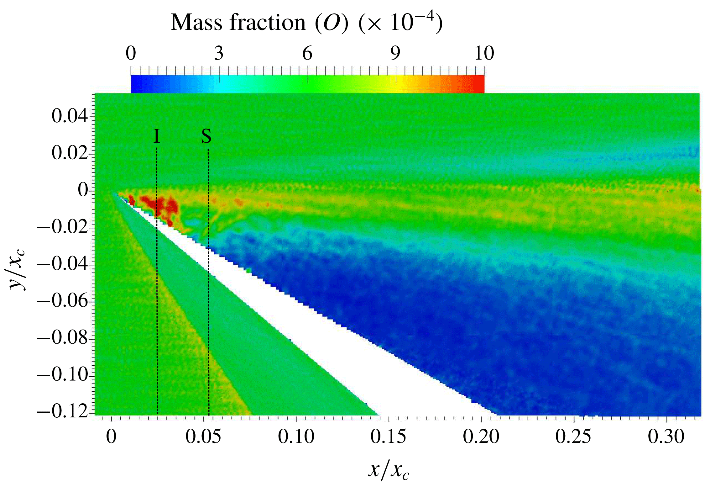
Since the vibrational temperature is frozen upstream of the leading edge (in the free stream), non-equilibrium at the leading edge is mainly manifested as a difference between translational and rotational temperatures. Close to the leading edge, dissociation brings down the vibrational temperature and it extends up to halfway between the beginning of the interaction (marked as $I$ ) and the separation locations. Owing to the free-molecular nature of the flow within the kinetic region, the flow characteristic is very diffuse so that the rotational temperature lags far below the translational value as a consequence of reduced collision frequency and only reaches equilibrium once it reaches the near-continuum denser flow interaction and separation regions. Based on the empirical correlation of Millikan & White (Reference Millikan and White1963) for vibrational–translational energy exchange, it is found that the vibrational relaxation times in the region closer to the wall and within the merged layer are of the order of $O$ (10 ms), whereas the corresponding cell residential times are of the order of $O$ (10 ns), which is based on velocity slip values and corresponding cell widths of the order of the free-stream MFP. This means that the vibration is essentially frozen, and changes in the vibrational temperature are brought about solely by the dissociation process. The vibrational temperature, after being reduced as a result of strong O $_{2}$ dissociation at the leading edge, requires many more collisions in order to change and, therefore, should relax slowly compared to the translational temperature. However, figure 10(a) shows a steady reduction in vibrational temperature between the end of the kinetic region and the beginning of the interaction, wherein the translational temperature remains nearly constant. The expansion process reduces the collision rate in this region and, as a result, no significant energy exchange occurs between the translational and other internal energy modes. At the same time, dissociation instigates a steady reduction in vibrational temperature in this region. The dissociation of O $_{2}$ reduces as the flow moves towards separation, while the collision rate increases, and the vibrational relaxation starts to occur more gradually, as it should occur as a result of vibrational–translational energy exchange.

3.2.3 Skin friction and gas velocity at the surface

These two surface parameters are discussed together so as to provide a better insight into discerning separation and reattachment locations on the surface. The traditional approach of identifying separation and reattachment as locations where the skin friction changes sign (positive to negative and vice versa) is not followed here. Rather, similar sign changes in the distribution of gas velocity at the surface ( $u_{gw}$ ), which in a molecular description corresponds to the average velocity of particles in the first layer of cells close to the surface, is chosen. The reason is as follows. In the continuum NS set of equations, shear stress is approximated as proportional to the first-order gradient of velocity and, therefore, it goes to zero at separation (and reattachment) as the velocity also goes to zero. In slip or transitional flow regimes, such linear first-order approximations become inadequate and higher-order terms become relevant. In DSMC, such higher-order effects are properly accounted for by computing the surface shear stress based on the overall tangential momentum difference between incident and reflected molecules in the first layer of cells. However, on a physical basis of momentum development, such inertial effects are felt only when the shear between fluid layers in a cell starts to be strongly altered by the adverse pressure gradient. Small perturbations in shear are masked in the overall momentum changes. On the other hand, $u_{gw}$ is based on the average directional flow of all particles in a cell, so that any change in flow direction is promptly reflected in its behaviour. In a well-separated flow, as in the present instance, differences between these two predictions of separation and reattachment based on $C_{f}$ and $u_{gw}$ distributions are not very significant. However, in the case of incipient and small separated flows, such differences can be significant (Prakash, Gai & O’Byrne Reference Prakash, Gai and O’Byrne2015) and $u_{gw}$ might be a better or the only possible parameter to determine the existence and size of separation. The behaviours of $C_{f}$ and $u_{gw}$ over the surface are shown in figure 12.

Figure 12.

Surface characteristics of (a) skin friction coefficient and (b) gas velocity. Gas velocity at the surface is normalised with respect to the free-stream velocity ( $u_{\infty }$ ).

From the leading edge, a steep fall in both properties occurs up to the separation location (see insets in figure 12). The non-dimensional separation locations based on the $u_{gw}$ distribution are 0.052 and 0.07, respectively, for sharp and blunt leading edges. The corresponding locations based on $C_{f}$ are 0.053 and 0.075, respectively. The prediction of reattachment locations, based on $u_{gw}$ and $C_{f}$ , are 2.715 and 2.716 for the sharp leading edge and 2.852 and 2.845 for the blunt leading edge. Thus, there is a good agreement in predictions of separation and reattachment from $C_{f}$ and $u_{gw}$ , as expected in a well-separated flow.

After separation, both $C_{f}$ and $u_{gw}$ stay negative due to the reverse flow in the recirculating region. Both change sign ( $-$ to $+$ ) close to the corner for the sharp case and midway along the expansion surface for the blunt case, indicating the formation of secondary vortices. Soon after the corner, the sign again changes ( $+$  to  $-$ ), indicating the downstream end of the secondary vortex. These effects are shown as insets in figure 12. Thereafter, $C_{f}$ steadily reduces to a minimum before starting to rise again just before reattachment, which is again represented by a change in sign ( $-$ to $+$ ). The two distinct local minima in $C_{f}$ , one after separation and the other just before reattachment, are a characteristic of large-scale separation. The peak of $C_{f}$ exhibits a double-lobed structure, which has also been found in no-slip NS computations (Khraibut et al. Reference Khraibut, Gai, Brown and Neely2017). At the same time, $u_{gw}$ is negative and stable after the corner and attains positive values after reattachment. It is interesting to note that, even after reattachment, there is some slip present. It has been commented by Bird (Reference Bird1994) that the slip velocity over the surface does not vanish completely but gradually reduces as the local flow-gradient-based Knudsen number ( $Kn_{grad}$ ) attains values less than 0.01.

There are some notable differences between the results. A few of these differences have already been addressed in §§ 3.2.1 and 3.2.2, such as the delay in separation and the downstream shift in reattachment and peak locations for the blunt leading edge. However, two unique characteristic differences between the models that show up in the $C_{f}$ and $u_{gw}$ distributions require further attention. Firstly, the magnitude of the local minimum just after separation is found to be larger for the sharp case. Secondly, with the sharp leading-edge case there is only a small secondary vortex in the close vicinity of the corner, whereas the blunt leading edge shows an extended secondary structure starting midway along the expansion surface and terminating just downstream of the corner. In order to ascertain the reasons for these differences, the behaviour of gas velocity at the surface close to the leading edge is examined.

The $u_{gw}$ distribution close to the leading edge for both cases is shown in figure 13, with regions delineated based on the discussion of figure 10. Within the kinetic region, a sharp rise in the gas velocity is observed from the leading edge due to collisionless flow and the increasing number of molecules colliding with the surface as the flow proceeds downstream along the surface. The rise continues until the merged layer. Unlike on a flat plate at zero angle of incidence, here the boundary layer development occurs within a strong viscous interactive environment characterised by rarefaction and thermal non-equilibrium. This results in a non-Blasius type of boundary layer growth.

Figure 13.

Gas velocity at the surface close to the leading edge for (a) sharp and (b) blunt cases.

A notable feature in figure 13 is the difference in magnitudes of gas velocity at the tip. For a blunt leading edge, the origin ( $x/x_{c}=0$ ) is chosen at the start of the flat expansion surface. Therefore, for the blunt case, fluid layers would be locally accelerated by the surface curvature of the hemispherical tip before the origin. This results in the incident molecules possessing higher kinetic energy within the kinetic region. At the same time, the peak value attained at the end of the kinetic region is lower for a blunt case. This is due to the stronger leading-edge shock moving upstream and resulting in a reduction in the extent of the kinetic region, which then limits the total number of incident molecules eventually interacting with the surface within this collisionless region. After the kinetic region, there is a continuous fall in velocity towards zero at separation for the sharp case. As explained earlier, due to the viscous energised lower layers of the boundary layer, the reduction in gas velocity at the wall is relatively gradual for the blunt case from the end of the kinetic region to the beginning of interaction. As a result, the upstream influence is felt further downstream at $x/x_{c}=0.035$ , compared to $x/x_{c}=0.025$ for the sharp leading edge. Even after the beginning of interaction, the overall energy increase in the boundary layer for a blunt leading edge offers larger resistance to the adverse pressure gradient and it starts to be seriously affected only after $x/x_{c}=0.045$ . This results in delayed separation at $x/x_{c}=0.07$ for the blunt leading edge (figure 12).

As explained previously, the strong entropy gradient region of the leading-edge shock extends only a small distance in the surface-normal direction and, therefore, generated disturbances get submerged progressively within the boundary layer as it grows. This results in a thicker boundary layer for the blunt case, as evidenced by the profile plots in figure 16(a) and 16(b). The thicker boundary layer at separation results in a stronger separation shock. The energy of the shear layer after separation is determined by the strength of the separation shock through which it traverses. The energy of the dividing streamline and layers close to it will be lower as they pass through a stronger separation shock, relative to a weaker separation shock in the sharp leading-edge case. The formation and evolution of the primary recirculation region is solely dependent on the energy supply from the outer inviscid flow through the shear layer. Therefore, when the shear layer is at a lower energy as a result of a stronger separation shock, less energy would be available to impart to the recirculation region. The outer streamlines of the primary recirculation region then attain a lower energy for the blunt case relative to the sharp case. These outer layers eventually flow closer to the surface by first turning parallel to the compression surface and then moving parallel to the expansion surface and towards separation. Reverse-flow streamlines encounter shear from the surface as well as adverse pressure from the corner and this can only be overcome by possessing a higher kinetic energy in the streamlines. So, the primary recirculation region of the blunt case with lower kinetic energy would result in breakdown of the primary recirculation into secondary and tertiary structures. On the contrary, the reverse-flow streamlines of the sharp case will have sufficient energy to overcome the shear and as a result the primary recirculation region is more stable. This higher energy is signified as larger negative values of $u_{gw}$ after separation for a sharp case relative to the blunt case in figure 12(b). The expansion of the secondary vortex at the corner and the breakdown of the primary recirculation region over the expansion surface to form tertiary vortex structures is illustrated in figure 14(b) for the blunt case.

Figure 14.

Streamlines superimposed on translational temperature contours for (a) sharp and (b) blunt cases. Separation and reattachment shocks are traced as dashed lines for better visualisation. A zoomed view of the secondary vortex is also shown.

3.3.1 Streamlines

Flow streamlines superimposed on the distribution of translational temperature are shown in figure 14 for both models. For better visualisation of the primary recirculation region, the domain is limited to the start of the reattachment shock. The propagation of the separation shock can be seen until it interacts with the reattachment shock, which starts slightly downstream of the reattachment. A triple point is formed by this interaction of separation and reattachment shocks (Edney type VI interaction), resulting in the emanation of expansion wavelets that impinge on the surface and cause the local reduction in surface parameters as discussed previously.

The most interesting aspect in streamline patterns is the structure of secondary and tertiary vortex formations. Only a single secondary vortex that is confined within the close vicinity of the corner is present for the sharp case. The blunt case not only has an expanded secondary vortex but also multiple tertiary vortex structures. In the direction of reverse flow, tertiary structures seem to develop gradually along the expansion surface. It originates as a trail of irregular structures starting just before the secondary vortex on the expansion surface and evolving into a pronounced shape halfway from the leading edge. The local changes in flow directions as a characteristic of these flow structures are well reflected in the behaviour of $C_{f}$ and $u_{gw}$ (see figure 12). It has been mentioned that the reason behind the formation of additional vortex structures in a blunt case, contrary to the sharp case, is due to lower flow energy of recirculation streamlines. It is, therefore, unable to overcome the shear at the wall and the adverse pressure from separation, thereby breaking down into smaller structures that characterise local separations. The flow mechanism that instigates such a reduction in reverse-flow energy will become apparent in the next section.

3.3.2 Vorticity

The vorticity distribution provides a better insight into the dissipative viscous energy transfer mechanism prevailing in the domain and is shown in figure 15.

Figure 15.

Vorticity distribution for (a) sharp and (b) blunt cases.

The shear layer forms a large vorticity sheet (of negative magnitude) between separation and reattachment. The primary recirculation region draws energy from the outer inviscid flow through this vorticity sheet. The outer streamlines of the primary recirculation region gain the maximum energy before the vorticity is continually reduced in the direction of the vortex core. However, the intensity of this energy transfer from the inviscid flow varies along the dividing streamline. A higher rate of energy transfer occurs at two locations: close to separation and at reattachment. Vorticity is high (of positive magnitude) in these locations due to the compression created by turning streamlines. Close to reattachment, this is also amplified by the growth of a reverse-flow boundary layer. These high-vorticity regions facilitate a higher rate of energy transfer from the inviscid side. Referring to figure 15(b), less energy would be available for infusing into recirculation streamlines from an outer flow that traverses a stronger separation shock as in the case of a blunt leading edge and, therefore, the total energy received by the recirculation region will be lower. The lower energy results in a faster dissipation due to shear from the wall as the reverse streamlines flow towards the corner from the reattachment. This is shown in figure 15(b), in which the large positive vorticity is seen to be dissipating as it approaches the corner. Meanwhile, this dissipation occurs very close to the corner for the sharp case, in which the reverse streamlines possess higher resistance against both shear from the wall and the adverse pressure from the corner. The dissipation effects are nothing but an energy feeding mechanism into the secondary vortex. Therefore, faster dissipation in the blunt case leads to an enhancement of the secondary structure.

In the blunt case, a large part of the reverse-flow energy is dissipated into the secondary structure and not much is left for the flow that proceeds over to the expansion surface. These streamlines will then not be able to overcome the shear over the expansion surface and result in breaking down into smaller tertiary vortices. For the sharp case, on the other hand, dissipative effects are smaller and therefore energy is carried to streamlines that proceed over to the expansion surface. Therefore, the reverse flow close to the surface has sufficient strength to withstand the shear and adverse pressure gradient from separation.

3.3.3 Flow profiles

It is interesting to examine the profiles of various flow parameters to analyse the spatial evolution of the flow. The chosen locations are at the beginning of interaction, at separation, at the corner and at reattachment. Firstly, let us examine the velocity profiles at these locations as shown in figure 16.

Figure 16.

Velocity profiles at (a) beginning of interaction, (b) separation, (c) corner and (d) reattachment.

Profiles at the beginning of interaction and separation exhibit significant differences between the cases. At the corner and at reattachment, relative variations are small and are expected due to the slight increase in the overall size of the respective recirculation regions and the resultant downstream shift in the reattachment location. At the beginning of the interaction, the gas velocity at the wall has a magnitude corresponding to approximately 15 % of the free-stream velocity for both cases. The boundary layer appears to be fuller for the sharp case. Typically, a fuller boundary layer possesses larger velocities close to the surface and a thinner subsonic layer, which reduces the upstream influence from adverse pressure gradients (Babinsky & Harvey Reference Babinsky and Harvey2013). This implies that the sharp leading edge should provide higher resistance to separation, but this is not the case seen here. The blunt leading edge with a less full profile is shown to have separation occurring further downstream than for the sharp case. The reason for this is the energising of the lower layers of the boundary layer due to viscous effects infused into the initial part of the boundary layer growth by a stronger leading-edge shock. This is reflected in the behaviour of surface-normal velocity gradients ( $\unicode[STIX]{x2202}u/\unicode[STIX]{x2202}s_{n}$ ) within a non-dimensional surface-normal distance of approximately 0.01 at the beginning of interaction. In this region, the gradients are larger for the blunt case but reduce further away from the surface, as the viscous effects then stimulate boundary layer thickening, which results in a thicker and less full profile. The profiles at separation also show a similar trend in the surface-normal velocity gradient within this distance. This gives the blunt leading edge higher resistance against separation even with an overall less full boundary layer growth. A thicker boundary layer at separation also leads to a stronger separation shock.

The comparison of pressure profiles at these locations is shown in figure 17. The pressure is not constant across the developing boundary layer from the leading edge to separation. The boundary layer growth leading to separation is affected by expansion and rarefaction, which results in a non-Blasius type of development. The pressure profiles are consistent with velocity profiles in that the blunt leading edge shows higher pressures corresponding to less full boundary layers at the beginning of interaction and separation. The larger bumps in pressure for the blunt leading edge indicate a stronger leading-edge shock. As observed in the velocity profile at the beginning of interaction, the surface-normal pressure gradients ( $\unicode[STIX]{x2202}p/\unicode[STIX]{x2202}s_{n}$ ) within a non-dimensional surface-normal distance of approximately 0.01 is smaller for the blunt leading edge and consistent with the higher surface-normal velocity gradients observed in this region. At the corner and at reattachment, the profiles for both cases are qualitatively the same but the magnitude is higher for the blunt case. This is due to the lower overall velocity in the recirculation region that consists of primary, secondary and tertiary vortex structures.

Figure 17.

Pressure profiles at (a) beginning of interaction, (b) separation, (c) corner and (d) reattachment.

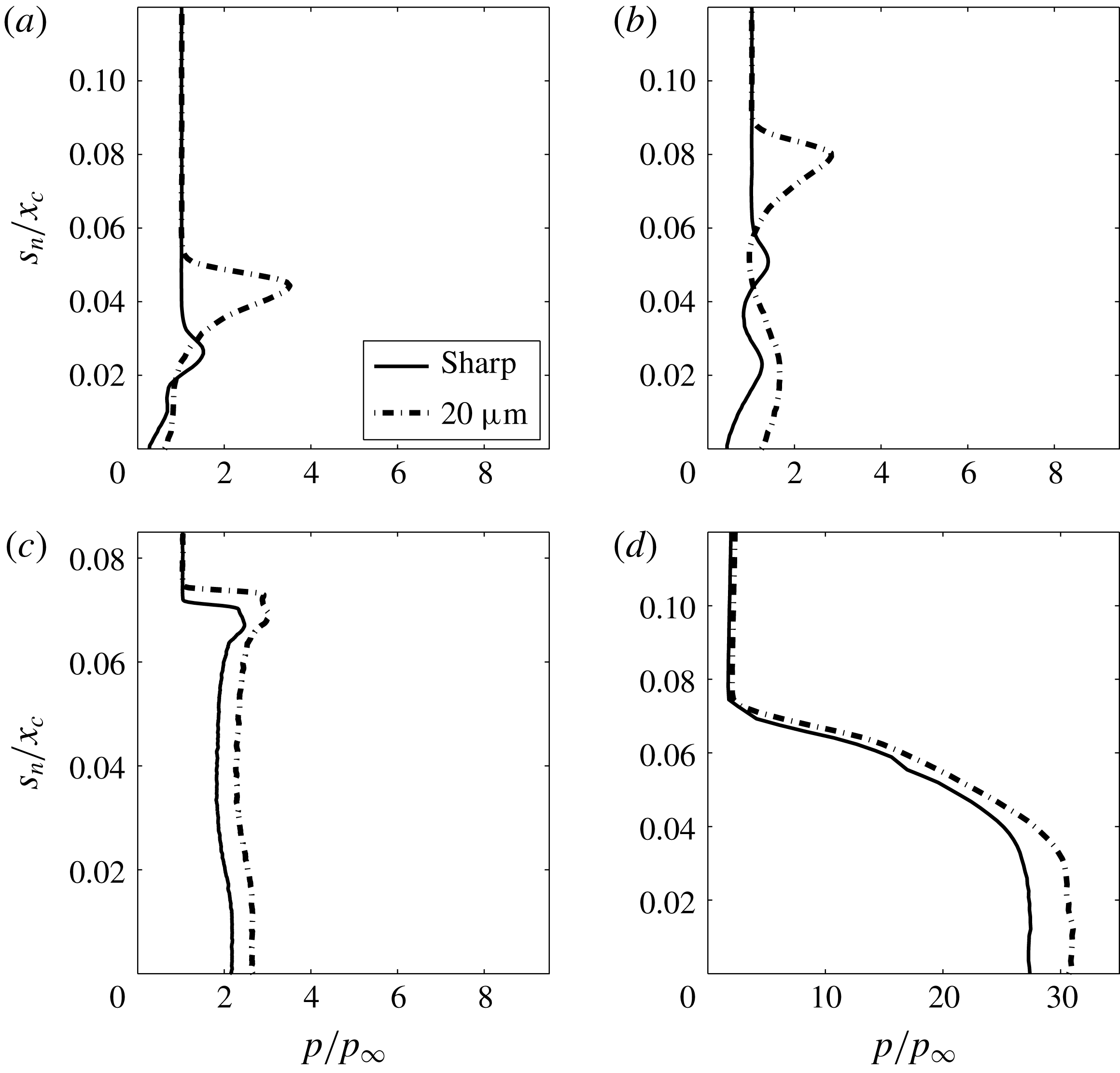
Similar to velocity and pressure, significant differences between temperature profiles are limited to the beginning of interaction and separation, as shown in figure 18. At the beginning of interaction, the temperature jump at the wall is 35 % lower for the blunt leading edge relative to the sharp case. At separation, it is only 18 % lower. Owing to the entropy generated by a stronger leading-edge shock in the blunt case, higher collisional interactions occur between molecules and the surface, as discussed in § 3.2.2 based on (3.4). The temperature jump, which is the average temperature of molecules in the first layer of cells close to the surface, is a resultant of the net contribution of heat imparted to the surface by the incoming molecules and that carried away from the surface by the reflected molecules. Such higher interactions between the incoming molecules and that of reflected molecules from the surface with an energy corresponding to the wall temperature result in the gas temperature jump being smaller for the blunt case relative to the sharp case. The entropy-enhanced viscous interactions for the blunt case push the location of the maximum in temperature further away from the surface and also make it smoother as well as wider. This makes the thermal boundary layer thicker for the blunt case. The differences are insignificant for the profiles at the corner and reattachment.

Figure 18.

Temperature profiles at (a) beginning of interaction, (b) separation, (c) corner and (d) reattachment.