1 Introduction
The problem of linear hydrodynamic stability is one of the canonical problems of fluid dynamics, and in particular there has been an enormous amount of research devoted to understanding the interplay between (statically stable) density variations and velocity shear since the seminal work of Helmholtz (Reference Helmholtz1868) and Kelvin (1871) that considered discontinuous distributions of velocity and density. The classical linear stability analysis of a shear layer of finite depth with an inflection point in velocity by Rayleigh (1880) and Fjortoft (Reference Fjortoft1950) has proved very useful for predicting the wavelength of the most unstable mode of linear theory. Dating at least to the pioneering work of Rosenhead (Reference Rosenhead1931), the finite-amplitude form of this so-called ‘Kelvin–Helmholtz’ instability (KHI) as an array of elliptical vortices ‘rolled up’ from the initial uniform strip of spanwise vorticity has been very widely observed in numerical simulation (see e.g. Moser & Rogers Reference Moser and Rogers1991), laboratory experiment (Thorpe Reference Thorpe1968) and the environment (see the recent data of van Haren et al. Reference van Haren, Gostiaux, Morozov and Tarakanov2014). Although the finite-amplitude ‘billow’ is prone to a rich array of secondary instabilities in both unstratified and stratified flows (Caulfield & Peltier Reference Caulfield and Peltier2000; Mashayek & Peltier Reference Mashayek and Peltier2012a ,Reference Mashayek and Peltier b ; Arratia, Caulfield & Chomaz Reference Arratia, Caulfield and Chomaz2013), the observational, numerical and experimental evidence is overwhelming that the finite-amplitude billow state is in some sense ‘robust’, in that a very broad range of initial conditions on an initially uniform shear layer are attracted to and ‘saturate’ as an array of elliptical billows for a non-trivial period of time.
As demonstrated by Holmboe (Reference Holmboe1962) and Hazel (Reference Hazel1972), a stable density stratification which varies over a length scale comparable to the depth of the shear layer reduces the linear growth rate of the primary KHI, although the effect of stable stratification on the ‘zoo’ of secondary instabilities and the subsequent dynamics during the transition to turbulence is significantly more subtle (Mashayek & Peltier Reference Mashayek and Peltier2012a
,Reference Mashayek and Peltier
b
; Mashayek, Caulfield & Peltier Reference Mashayek, Caulfield and Peltier2013). However, if the density distribution is ‘sharp’, in that the density distribution varies over a substantially shorter length scale
 $\unicode[STIX]{x1D6FF}$
than the scale
 $h$
over which the velocity varies, a qualitatively different linear instability is possible, known as ‘Holmboe waves’, or the ‘Holmboe instability’, and first predicted by Holmboe (Reference Holmboe1962). We will refer to this instability subsequently as the ‘Holmboe wave instability’ or HWI.
For sharp density distributions, the KHI is still predicted to occur for a range of wavenumbers when the density interface is ‘weak’, in the sense that the bulk Richardson number
 $Ri_{B}$
is sufficiently small, where
 $Ri_{B}$
is defined as
 $$\begin{eqnarray}Ri_{B}=\frac{g\unicode[STIX]{x0394}\unicode[STIX]{x1D70C}h}{\unicode[STIX]{x1D70C}_{0}\unicode[STIX]{x0394}U^{2}},\end{eqnarray}$$
where
 $g$
is the acceleration due to gravity,
 $\unicode[STIX]{x0394}\unicode[STIX]{x1D70C}$
is the total density jump across the density interface of depth
 $\unicode[STIX]{x1D6FF}$
,
 $\unicode[STIX]{x1D70C}_{0}$
is a reference density (with
 $\unicode[STIX]{x1D70C}_{0}\gg \unicode[STIX]{x0394}\unicode[STIX]{x1D70C}$
so that the Boussinesq approximation applies, for simplicity), and the velocity difference
 $\unicode[STIX]{x0394}U$
occurs over a shear layer with characteristic depth
 $h\gg \unicode[STIX]{x1D6FF}$
. However, as
 $Ri_{B}$
increases, eventually a bifurcation occurs and the flow becomes unstable (for a range of wavenumbers) to the qualitatively different HWI. Typically there continues to be a range of wavenumbers which are unstable to the HWI for all
 $Ri_{B}$
, with the range narrowing and moving to higher mean wavenumber as
 $Ri_{B}$
increases.
Also, unlike the KHI, which has a real phase velocity equal to the mean velocity of the shear layer, the HWI has a non-zero phase speed. If the flow is symmetric about the midpoint of the shear layer, there are two such instabilities with equal growth rates and equal and opposite phase speeds localized above and below the density interface. If the flow is asymmetric, one of the instabilities will dominate, as discussed by Lawrence, Browand & Redekopp (Reference Lawrence, Browand and Redekopp1991). The finite-amplitude manifestation of this instability was observed experimentally first qualitatively by Thorpe (Reference Thorpe1968), and numerically in detail by Smyth, Klaasen & Peltier (Reference Smyth, Klaasen and Peltier1988), and takes the form of propagating vortices localized at the linear instability’s critical layer, which induce a cusping of the strong density interface (see for example Tedford, Pieters & Lawrence (Reference Tedford, Pieters and Lawrence2009) and Carpenter et al. (Reference Carpenter, Tedford, Rahmani and Lawrence2010b ) for more recent experimental observations and numerical simulations). Unlike the KHI, which rolls up and overturns a relatively weak density interface, the HWI scours the interface, and so appears to have different mixing properties (Smyth & Winters Reference Smyth and Winters2003; Meyer & Linden Reference Meyer and Linden2014; Salehipour, Caulfield & Peltier Reference Salehipour, Caulfield and Peltier2016). Nevertheless, the HWI may also be thought of as ‘robust’, in that it has been widely observed experimentally (see for example Zhu & Lawrence Reference Zhu and Lawrence2001; Tedford et al. Reference Tedford, Pieters and Lawrence2009; Meyer & Linden Reference Meyer and Linden2014) and numerically (see for example Smyth et al. Reference Smyth, Klaasen and Peltier1988; Carpenter et al. Reference Carpenter, Tedford, Rahmani and Lawrence2010b ; Salehipour et al. Reference Salehipour, Caulfield and Peltier2016) to survive for a substantial time.
As has been reviewed by Carpenter et al. (Reference Carpenter, Tedford, Heifetz and Lawrence2011) (see also Sutherland Reference Sutherland2010), the physical mechanism underlying these instabilities can be interpreted as arising due to Doppler-shifted interaction between marginally stable waves localized either at the edge of the shear layer, or at the density interface, an interpretation which has been presented by many authors in various contexts (see for example Bretherton Reference Bretherton1966; Cairns Reference Cairns1979). It appears to have originally been proposed in the long-wave limit by Taylor in his 1915 Adams prize essay entitled ‘Turbulent motions in fluids’ (unfortunately the original manuscript of this essay held in the library of Trinity College, Cambridge is missing the relevant chapter) and reported subsequently in Taylor (Reference Taylor1931) along with his derivation of the ‘Taylor–Goldstein equation’, which describes the linear stability properties of an inviscid stratified shear flow. The equation was independently derived by Goldstein (Reference Goldstein1931) and Haurwitz (Reference Haurwitz1931) (see Craik (Reference Craik1988) for a fuller discussion).
At the edge of a shear layer, where the spanwise vorticity is varying rapidly, a vorticity wave sometimes referred to as a ‘Rayleigh wave’ or ‘Rossby edge wave’ is localized. The classical KHI may be interpreted as arising from the two vorticity waves at either edge of the shear layer being appropriately Doppler-shifted by the prevailing flow such that they have the same phase speed, thus ‘interacting’ in the sense described by Carpenter et al. (Reference Carpenter, Tedford, Heifetz and Lawrence2011). Analogously, the HWI may be interpreted as being an instability which only occurs in the presence of density stratification, as it arises through an interaction between an internal gravity wave on the sharp density interface and one of the vorticity waves at the edge of the shear layer.
However, as noted by Taylor (Reference Taylor1931), it is not necessary for stratified shear instabilities to rely on interactions with vorticity waves, or equivalently on the presence of a finite-depth shear layer. Taylor considered various scenarios with more than two density interfaces in the presence of uniform shear, and so the unstratified flow is stable. In the simplest case, the density distribution is arranged in three layers, with an intermediate layer of finite depth
 $d$
between two outer layers. In this case there are two density interfaces on which internal gravity waves can propagate. Due to Doppler-shifting by the background shear, it is then possible for internal waves on the two density interfaces to interact, leading to the prediction of another, inherently stratified instability.
When the intermediate layer is actually embedded within a finite-depth shear layer, Caulfield (Reference Caulfield1994) demonstrated that both the Taylor instability and the HWI are predicted to be unstable in different wavenumber bands for a fixed value of
 $Ri_{B}$
, with these bands being a function of the ratio
 $d/h$
of the depth of the intermediate layer to the depth of the shear layer. Caulfield et al. (Reference Caulfield, Peltier, Yoshida and Ohtani1995) considered such a three-layer flow experimentally, and appeared to observe, at least qualitatively, both Taylor instabilities and HWI simultaneously for appropriate values of the ratio
 $d/h$
. Perhaps to distinguish it from other instabilities associated with G. I. Taylor, Carpenter, Balmforth & Lawrence (Reference Carpenter, Balmforth and Lawrence2010a
) referred to this instability as the ‘Taylor–Caulfield’ instability, a nomenclature which has also been used several times recently (see e.g. Mashayek & Peltier Reference Mashayek and Peltier2013; Guha & Lawrence Reference Guha and Lawrence2014; Heifetz & Mak Reference Heifetz and Mak2015; Churilov Reference Churilov2016). Therefore, we will refer to this instability as the TCI. In the experiments of Caulfield et al. (Reference Caulfield, Peltier, Yoshida and Ohtani1995) it proved challenging to observe the finite-amplitude manifestation of the TCI, as it is localized in the intermediate layer, which was typically intensely dyed. Furthermore, the experimental design was such that the depth of the intermediate layer slowly decreased with time, making it difficult to determine quantitatively the base flow on which the observed structures had been unstable.
Such a multi-layer density distribution was also simulated numerically by Lee & Caulfield (Reference Lee and Caulfield2001) with a steady, two-dimensional base flow, and they made two key observations. First, the finite-amplitude manifestation of the primary TCI, although it is inherently a stratified instability and relies completely on the presence of sheared neighbouring density interfaces, bears a superficial resemblance to a KHI in that it takes the form of a connected array of elliptical vortices. Second, even in two dimensions at relatively low Reynolds number, they observed that the TCI was prone to strong secondary instabilities due to the intense baroclinic vorticity generation associated with the primary TCI elliptical vortices strongly perturbing the bounding density interfaces.
Such susceptibility to strong secondary instabilities was also observed by Balmforth, Roy & Caulfield (Reference Balmforth, Roy and Caulfield2012), who considered a reduced, long-wave asymptotic ‘stratified defect’ model to consider the two-dimensional finite-amplitude behaviour of such layered stratified shear flows. Instabilities which could be identified as being of TCI type and HWI type grew to finite amplitude using this reduced model, although it is important to remember that the governing equations in this system are not the full Boussinesq Navier–Stokes equations. Nevertheless, Balmforth et al. (Reference Balmforth, Roy and Caulfield2012) also noted the interesting and somewhat surprising phenomenon of ‘parasitic’ secondary HWI, which in certain circumstances appear to destroy the primary TCI relatively rapidly.
These numerical calculations lead to the possibility of an alternative interpretation of the experiments discussed in Caulfield et al. (Reference Caulfield, Peltier, Yoshida and Ohtani1995). They argued that the observation of TCI and HWI was consistent with the theoretical predictions of Caulfield (Reference Caulfield1994); i.e. that effectively in some parameter ranges the TCI and the HWI could both grow and saturate as primary instabilities in parallel, each with a different characteristic phase speed, and localized at a different height within the flow. This is somewhat at odds with the conventional received wisdom that it is to be expected experimentally and numerically that the most unstable mode of linear theory will grow to dominate the nonlinear finite-amplitude evolution of an unstable flow. However, numerical simulations are typically constructed with periodic streamwise boundary conditions, thus enforcing a quantization of accessible streamwise wavenumbers. As demonstrated by Scinocca & Ford (Reference Scinocca and Ford2000), multiple wavenumbers of KHI with slightly different wavenumbers can grow to finite amplitude in sufficiently long computational domains, and so it is at least conceivable that qualitatively different primary instabilities with different growth mechanisms and localized at different heights within the flow can co-exist at finite amplitude when the boundary conditions allow.
The numerical calculations of Lee & Caulfield (Reference Lee and Caulfield2001), however, suggest a note of caution, in that the primary TCI was prone to very strong secondary instabilities, at least some of which could modify the base flow in such a way as to induce the development of secondary HWI in series, consistently with the observations of Balmforth et al. (Reference Balmforth, Roy and Caulfield2012).
Taylor (Reference Taylor1931) explained the delay in publishing his theoretical predictions at least in part because he was unable to ‘undertake experiments designed to verify, or otherwise, the results’, thus suggesting that he found it difficult to observe the finite-amplitude manifestation of the TCI. There has been renewed interest in the TCI recently, not least because of the formalization and extension of the wave interaction theory to include transient growth phenomena in the linear regime (Guha & Lawrence Reference Guha and Lawrence2014). Furthermore, evidence is mounting that, over a wide range of stratified turbulent mixing processes (see e.g. Brethouwer et al. Reference Brethouwer, Billant, Lindborg and Chomaz2007; Oglethorpe, Caulfield & Woods Reference Oglethorpe, Caulfield and Woods2013; Mashayek et al. Reference Mashayek, Caulfield and Peltier2013), layering of the density field is generic. As originally predicted by Phillips (Reference Phillips1972), turbulence in a stratified fluid typically leads to the development of relatively deep, relatively well-mixed layers separated by thin interfaces of substantially enhanced density gradient. Such layered density profiles are precisely those which are predicted to be susceptible to the TCI if a larger scale shear is imposed, which is conceivable in the geophysical context.
Therefore, it seems natural to attempt to address three outstanding questions concerning the properties of layered stratified shear flow, and answering these questions is the aim of this article. First, we wish to determine whether the finite-amplitude manifestation of a primary TCI is robust, in the sense that it saturates at a finite amplitude for a sufficiently long time such that its finite-amplitude form might possibly be observed in the laboratory or in nature. Second, we wish to investigate whether it is possible to observe two qualitatively different primary instabilities, an observation which would give further weight to the interpretation of the experiments of Caulfield et al. (Reference Caulfield, Peltier, Yoshida and Ohtani1995) in light of the primary instability argument presented by Caulfield (Reference Caulfield1994). Finally, we wish to determine if the series development of secondary HWI does not depend on the reduced stratified defect model developed in Balmforth et al. (Reference Balmforth, Roy and Caulfield2012), such that the breakdown of a TCI as a solution to the full Navier–Stokes equations actually can lead in an inherently secondary fashion to propagating cusped waves characteristic of the HWI.
To address these three questions, we consider the linear stability properties and nonlinear evolution of two-dimensional plane Couette flow (PCF) with an initial three-layer density distribution. The fluid layer has total depth
 $2h$
between two horizontal plates, which are driven at constant velocity
 $\pm \unicode[STIX]{x0394}U$
, so that the initial velocity distribution has purely linear shear. Therefore, in PCF, there is no identifiable ‘shear layer’ with constant velocity outside, nor an inflection point in the velocity profile, and it is well known (Romanov Reference Romanov1973) that if the fluid is unstratified, there is no linear instability of this flow for all Reynolds numbers. However, as originally demonstrated by Huppert (Reference Huppert1973), statically stable density distributions can actually linearly destabilize this flow.
Therefore, this velocity profile is particularly well-suited to investigating the properties of the TCI without the complicating presence of inherently unstratified instabilities such as the KHI. In particular, any primary instability identified with phase speed equal to the mean (zero) flow at the midpoint of the fluid layer is not classifiable as a KHI, but rather may be classified as a TCI. However, an undoubted disadvantage of this flow geometry is that there is no finite-depth shear layer. Therefore, one of the key components for a classical HWI is missing, namely the existence of a vorticity wave localized at the edge of the finite-depth shear layer. However, as we discuss in more detail below, when the flow is at finite Reynolds number, a no-slip boundary condition for the perturbation horizontal velocity applies, which crucially can support a stress at the channel wall, and hence non-zero perturbation vorticity. This inherently viscous process allows for the development of propagating vortical perturbations localized very close to the two walls which appear to play an analogous role to the above-mentioned vorticity waves, in the sense that they can interact with internal waves localized on density interfaces to lead to an instability which is at least analogous to the classical HWI. It is important to appreciate that this analogous process can only occur at finite Reynolds number, and so any such instability should be classified as an inherently viscous instability. Such an inherently viscous stratified instability due to the introduction of no-slip boundary conditions in the absence of any other instability mechanism was hypothesized to exist by Lindzen & Barker (Reference Lindzen and Barker1985) as a stratified equivalent of the critical layer over-reflection explanation of the linear instability of unstratified viscous plane Poiseuille flow by Lindzen & Rambaldi (Reference Lindzen and Rambaldi1986). However, to the current authors’ knowledge this is the first time such instability has been identified and investigated.
For simplicity, we consider a three-layer density distribution where initially the three layers have equal depth
 $2h/3$
and densities
 $\unicode[STIX]{x1D70C}_{0}+\unicode[STIX]{x0394}\unicode[STIX]{x1D70C}$
,
 $\unicode[STIX]{x1D70C}_{0}$
and
 $\unicode[STIX]{x1D70C}_{0}-\unicode[STIX]{x0394}\unicode[STIX]{x1D70C}$
, such that
 $\unicode[STIX]{x1D70C}_{0}\gg \unicode[STIX]{x0394}\unicode[STIX]{x1D70C}$
, and so the Boussinesq approximation applies.
In § 2, we define the specific characteristics of this flow, particularly clarifying the properties of the interfaces between the three layers, and the appropriate definition of the various non-dimensional parameters. In § 3, we perform two linear stability analyses: first for the analytically tractable case of an inviscid, non-diffusive, three-layer fluid with a discontinuous stratification; and second for a viscous fluid with a diffusive, smooth density profile. For the discontinuous stratification we identify only primary TCI as expected, while for the finite-Reynolds-number flows we find both primary TCI and the above-mentioned inherently viscous non-zero phase speed instabilities reminiscent of the HWI, which we thus choose to refer to as VHWI. Interestingly, we find that the existence of different branches of primary TCI has a non-monotonic dependence on Reynolds number of the global largest linear growth rate (maximized across all wavenumbers and bulk Richardson numbers).
By application of a theorem originally due to Yih (Reference Yih1955), we can verify that this base flow is nevertheless subject to two-dimensional rather than three-dimensional primary instabilities. Therefore, we restrict our attention here to two-dimensional simulations. Although real flows are of course three-dimensional, the nonlinear evolution of flows susceptible to primary TCI is very poorly understood, not least because the TCI appears to require ‘sharp’ density interfaces with substantial computational demands associated with, for example, high values of Prandtl and Reynolds number (
 $Pr$
and
 $Re$
), even in two-dimensional flows. We devote § 4 to a discussion of two-dimensional nonlinear numerical simulations of this base flow at two sets of parameter values, one corresponding to the global maximum of growth rate for the primary TCI at
 $Pr=\unicode[STIX]{x1D708}/\unicode[STIX]{x1D705}=300$
, which occurs at
 $Re=Uh/\unicode[STIX]{x1D708}=600$
(
 $\unicode[STIX]{x1D708}$
is the kinematic viscosity of the fluid and
 $\unicode[STIX]{x1D705}$
is the molecular diffusivity of the density field) and one at appreciably higher Reynolds number,
 $Re=5000$
and
 $Pr=70$
, which serves as an approximation to the
 $Re\rightarrow \infty$
limit. These two simulations have been specifically selected to address our second and third aims. For
 $Re=600$
and
 $Pr=300$
, there is predicted both a primary TCI and a primary VHWI with the same wavenumber (but different growth rates and phase speeds) which can in principle co-exist in parallel in the same periodic domain. Conversely, for
 $Re=5000$
and
 $Pr=70$
, only a primary TCI is predicted to occur in the chosen periodic domain. However, in this case, there is the possibility of substantial modification of the density and velocity distributions, in particular leading to the development of intensified shear layers in the vicinity of the density interfaces, thus triggering the series development of a secondary, yet classical inviscid HWI, as observed by Balmforth et al. (Reference Balmforth, Roy and Caulfield2012).
The results at both parameter sets demonstrate conclusively that the primary TCI is not at all robust, and it is not appropriate to consider that this instability ‘saturates’ (and remains) at finite amplitude for any significant period. As the primary TCI is destroyed by the background shear, strongly Reynolds-number-dependent secondary processes arise associated with the strong baroclinic generation of vorticity due to the deflection of the density interfaces by the development of the primary TCI. At
 $Re=600$
, there is clear evidence of the eventual emergence of the primary VHWI, whereas at
 $Re=5000$
, analogously to the stratified defect results of Balmforth et al. (Reference Balmforth, Roy and Caulfield2012), the decay of the TCI modifies the horizontally averaged base flow in a way which is conducive to the secondary development of ‘parasitic’ classical HWI. Our simulations thus suggest that HWI are highly likely to occur in layered flows, either as primary or secondary instabilities, and that the TCI is a very ‘fragile’ instability, prone to vigorous secondary instabilities, even in two dimensions. We discuss this issue further and draw our conclusions in § 5.
2 Flow geometry
We consider a two-dimensional three-layer Boussinesq fluid in a PCF geometry, so that we have background dimensional velocity and density profiles given by
 $$\begin{eqnarray}\displaystyle \boldsymbol{U}^{\ast }(y^{\ast })=\unicode[STIX]{x0394}Uy^{\ast }\hat{\boldsymbol{x}},\quad \bar{\unicode[STIX]{x1D70C}}^{\ast }(y)=\unicode[STIX]{x1D70C}_{0}-\unicode[STIX]{x0394}\unicode[STIX]{x1D70C}\left[\tanh \frac{R}{h}(y^{\ast }-h/3)+\tanh \frac{R}{h}(y^{\ast }+h/3)\right], & & \displaystyle \nonumber\\ \displaystyle & & \displaystyle\end{eqnarray}$$
where
 $y^{\ast }\in [-h,h]$
is the vertical coordinate, and asterisks denote dimensional quantities. The density profile is a smooth transition between the statically stable three-layer stratification
 $\unicode[STIX]{x1D70C}_{0}-\unicode[STIX]{x0394}\unicode[STIX]{x1D70C}$
,
 $\unicode[STIX]{x1D70C}_{0}$
and
 $\unicode[STIX]{x1D70C}_{0}+\unicode[STIX]{x0394}\unicode[STIX]{x1D70C}$
, with the sharpness of transition measured by the parameter
 $R$
. We expect that this base flow will be susceptible to a primary TCI.
We consider two-dimensional perturbations around the base flow, so that the total velocity and density fields are
 $$\begin{eqnarray}\boldsymbol{u}_{tot}^{\ast }=\boldsymbol{U}^{\ast }(y^{\ast })+\boldsymbol{u}^{\ast }(x^{\ast },y^{\ast },t^{\ast }),\quad \unicode[STIX]{x1D70C}_{tot}^{\ast }=\bar{\unicode[STIX]{x1D70C}^{\ast }}(y^{\ast })+\unicode[STIX]{x1D70C}^{\ast }(x^{\ast },y^{\ast },t^{\ast }),\end{eqnarray}$$
with the boundary conditions
 $\boldsymbol{u}^{\ast }=0$
and
 $\unicode[STIX]{x1D70C}^{\ast }=0$
at
 $y^{\ast }=\pm h$
. Using
 $h$
,
 $\unicode[STIX]{x0394}U$
and
 $\unicode[STIX]{x0394}\unicode[STIX]{x1D70C}$
to non-dimensionalize, we obtain the following equations of motion for the Boussinesq fluid
 $$\begin{eqnarray}\displaystyle & \displaystyle \frac{\unicode[STIX]{x2202}\boldsymbol{u}}{\unicode[STIX]{x2202}t}+(\boldsymbol{u}+\boldsymbol{U})\boldsymbol{\cdot }\unicode[STIX]{x1D735}(\boldsymbol{u}+\boldsymbol{U})=-\unicode[STIX]{x1D735}p-Ri_{B}\unicode[STIX]{x1D70C}\hat{\boldsymbol{y}}+\frac{1}{Re}\unicode[STIX]{x1D6FB}^{2}\boldsymbol{u}, & \displaystyle\end{eqnarray}$$
 $$\begin{eqnarray}\displaystyle & \displaystyle \frac{\unicode[STIX]{x2202}\unicode[STIX]{x1D70C}}{\unicode[STIX]{x2202}t}+(\boldsymbol{u}+\boldsymbol{U})\boldsymbol{\cdot }\unicode[STIX]{x1D735}(\unicode[STIX]{x1D70C}+\bar{\unicode[STIX]{x1D70C}})=\frac{1}{RePr}\unicode[STIX]{x1D6FB}^{2}\unicode[STIX]{x1D70C}, & \displaystyle\end{eqnarray}$$
 $$\begin{eqnarray}\displaystyle & \displaystyle \unicode[STIX]{x1D735}\boldsymbol{\cdot }\boldsymbol{u}=0, & \displaystyle\end{eqnarray}$$
with boundary conditions
 $$\begin{eqnarray}\boldsymbol{u}(y=\pm 1)=0,\quad \unicode[STIX]{x1D70C}(y=\pm 1)=0,\end{eqnarray}$$
where the Reynolds number
 $Re$
, Prandtl number
 $Pr$
and bulk Richardson number
 $Ri_{B}$
are given by
 $$\begin{eqnarray}Re=\frac{\unicode[STIX]{x0394}Uh}{\unicode[STIX]{x1D708}},\quad Pr=\frac{\unicode[STIX]{x1D708}}{\unicode[STIX]{x1D705}},\quad Ri_{B}=\frac{g\unicode[STIX]{x0394}\unicode[STIX]{x1D70C}h}{\unicode[STIX]{x1D70C}_{0}\unicode[STIX]{x0394}U^{2}}.\end{eqnarray}$$
We note that the perturbation vorticity
 $\unicode[STIX]{x1D74E}=\unicode[STIX]{x1D714}\hat{\boldsymbol{z}}$
is defined by
 $$\begin{eqnarray}\unicode[STIX]{x1D714}=\frac{\unicode[STIX]{x2202}v}{\unicode[STIX]{x2202}x}-\frac{\unicode[STIX]{x2202}u}{\unicode[STIX]{x2202}y}.\end{eqnarray}$$
Therefore, at the horizontal channel walls at
 $y=\pm 1$
, where
 $u=v=0$
, it is still possible for
 $\unicode[STIX]{x1D714}(\pm 1)\neq 0$
, since the second term on the right-hand side of (2.8) can in general be non-zero at finite
 $Re$
. As we discuss in more detail below, such non-zero wall-localized vorticity at finite
 $Re$
plays a central role in the development of primary non-zero phase speed instabilities for flows with finite
 $Re$
.
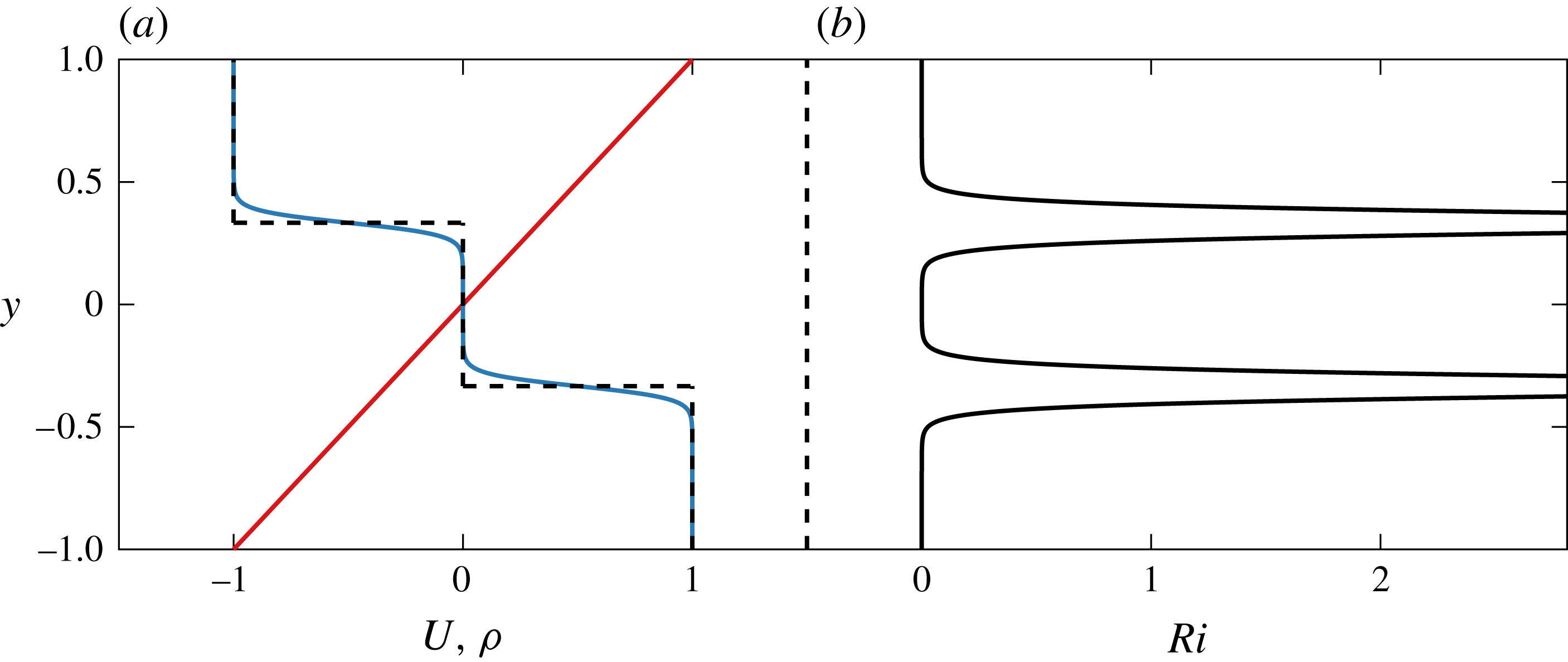
In figure 1 we plot the non-dimensional streamwise base velocity distribution
 $U(y)$
and the initial base density distribution
 $\bar{\unicode[STIX]{x1D70C}}(y)-\unicode[STIX]{x1D70C}_{0}/\unicode[STIX]{x0394}\unicode[STIX]{x1D70C}$
for
 $R=20$
and
 $R\rightarrow \infty$
, where
 $$\begin{eqnarray}\boldsymbol{U}(y)=U(y)\boldsymbol{x}=y\hat{\boldsymbol{x}},\quad \bar{\unicode[STIX]{x1D70C}}(y)-\frac{\unicode[STIX]{x1D70C}_{0}}{\unicode[STIX]{x0394}\unicode[STIX]{x1D70C}}=-\frac{1}{2}[\tanh R(y-1/3)+\tanh R(y+1/3)].\end{eqnarray}$$
(a) Vertical variation of base flow velocity
 $U(y)$
(red), base flow density distribution
 $\bar{\unicode[STIX]{x1D70C}}(y)-\unicode[STIX]{x1D70C}_{0}/\unicode[STIX]{x0394}\unicode[STIX]{x1D70C}$
with
 $R=20$
(blue) and
 $R\rightarrow \infty$
(dashed line) as defined in (2.9a,b
). (b) Vertical variation of gradient Richardson number
 $Ri(y)$
as defined in (2.10) for the base flow density distribution with
 $R=20$
shown in (a). The maximum value
 $Ri(\pm 1/3)=5.22$
.

The gradient Richardson number
 $Ri(y)$
is defined as
 $$\begin{eqnarray}Ri(y)\equiv -Ri_{B}\frac{{\displaystyle \frac{\unicode[STIX]{x2202}\unicode[STIX]{x1D70C}_{tot}}{\unicode[STIX]{x2202}y}}}{\left({\displaystyle \frac{\unicode[STIX]{x2202}u_{tot}}{\unicode[STIX]{x2202}y}}\right)^{2}},\end{eqnarray}$$
and so, for the base flow defined by (2.9a,b ),
 $$\begin{eqnarray}Ri(y)=\frac{Ri_{B}R}{2}\left[\text{sech}^{2}R(y-1/3)+\text{sech}^{2}R(y+1/3)\right],\end{eqnarray}$$
which is very close to zero for a large range of
 $y$
for all bulk Richardson numbers
 $Ri_{B}$
. Specifically, there are broad regions of the flow for which
 $Ri(y)<1/4$
, and so by the Miles–Howard theorem (Howard Reference Howard1961; Miles Reference Miles1961) there is at least the possibility of linear instability for all values of
 $Ri_{B}$
.
3 Linear stability analysis
3.1 Stability of step-like profiles in the
 $Re\rightarrow \infty$
,
$R\rightarrow \infty$
limit


Before investigating the full linear problem at finite
 $Re$
, we perform a linear stability analysis on the simpler background density field that consists of step-like layers in the density profile, shown in figure 1(a) with a dashed line, making the further assumptions that both
 $Re\rightarrow \infty$
and
 $RePr\rightarrow \infty$
. As reviewed in Carpenter et al. (Reference Carpenter, Tedford, Heifetz and Lawrence2011), such profiles allow substantial analytical progress to be made as the eigenvalue problem to determine the growth rate of normal modes reduces to the solution of a polynomial equation. This simplified problem retains many of the key features of the full, finite-
 $Re$
problem.
We consider normal mode perturbations to the base flow of the form
 $$\begin{eqnarray}(\boldsymbol{u},\unicode[STIX]{x1D70C})=[\hat{\boldsymbol{u}}(y),\hat{\unicode[STIX]{x1D70C}}(y)]\exp (\text{i}\unicode[STIX]{x1D6FC}[x-ct]),\quad \unicode[STIX]{x1D6FC}=kh,\quad \unicode[STIX]{x1D70E}=\unicode[STIX]{x1D6FC}c_{i},\quad \boldsymbol{u}=\unicode[STIX]{x1D735}\times \unicode[STIX]{x1D713},\end{eqnarray}$$
where
 $\unicode[STIX]{x1D713}$
is the streamfunction,
 $\unicode[STIX]{x1D6FC}$
is the non-dimensional wavenumber, assumed to be real and non-negative without loss of generality, and
 $c=c_{r}+ic_{i}$
is the (in general) complex phase speed, such that
 $\unicode[STIX]{x1D70E}$
is the growth rate of the linear normal mode. Considering such infinitesimal perturbations to the base flow defined in (2.9a,b
), the linearized form of (2.5) (with
 $Re\rightarrow \infty$
and
 $RePr\rightarrow \infty$
) can be reduced to the appropriate form of the (inviscid) Taylor–Goldstein equation for the streamfunction eigenfunction
 $\hat{\unicode[STIX]{x1D713}}(y)$
,
 $$\begin{eqnarray}\frac{\text{d}^{2}\hat{\unicode[STIX]{x1D713}}}{\text{d}y^{2}}-\unicode[STIX]{x1D6FC}^{2}\hat{\unicode[STIX]{x1D713}}+\frac{N^{2}\hat{\unicode[STIX]{x1D713}}}{(y-c)^{2}}=0,\quad N^{2}=-Ri_{B}\frac{\text{d}\bar{\unicode[STIX]{x1D70C}}}{\text{d}y}.\end{eqnarray}$$
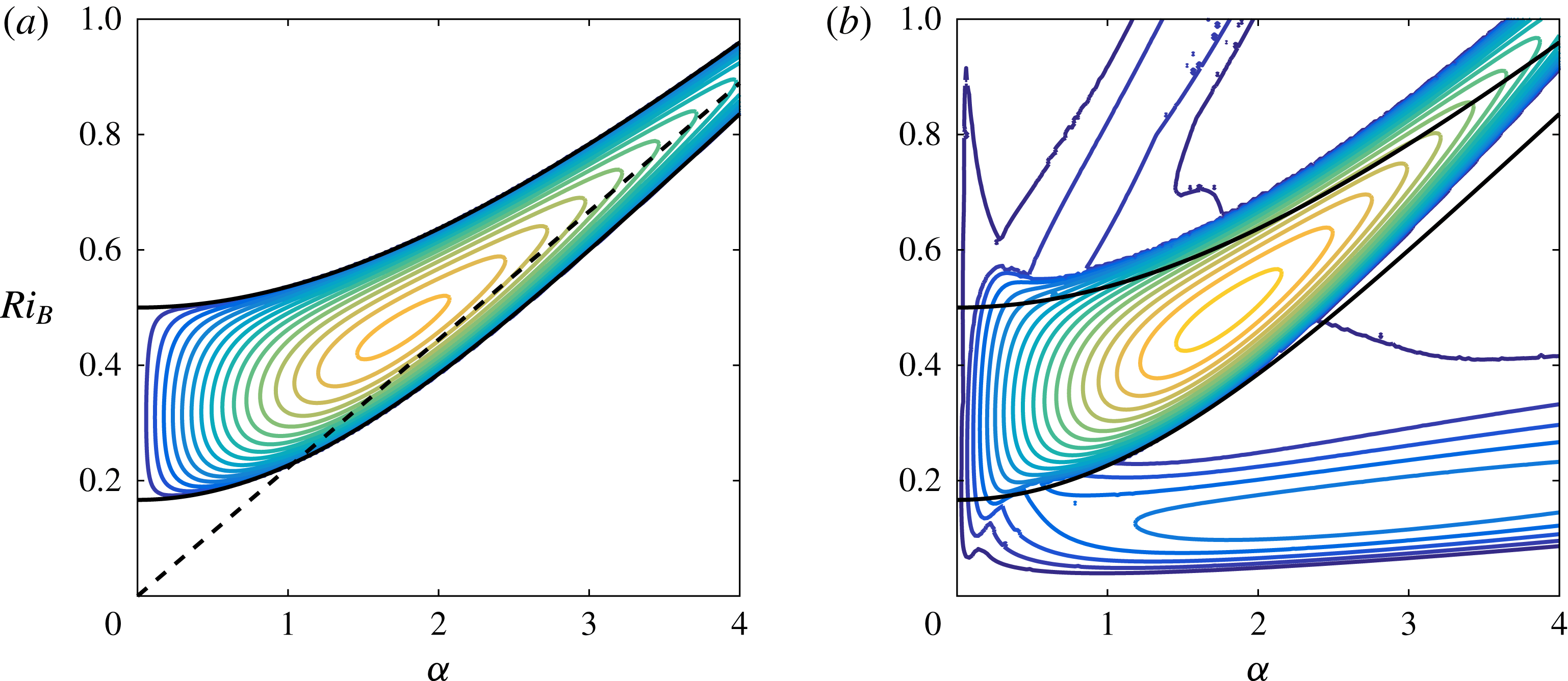
(a) Contours of growth rate
 $\unicode[STIX]{x1D70E}$
for the inviscid, non-diffusive step-like density profile with dispersion relation given by (3.4a,b
). The dashed line shows the large-
 $\unicode[STIX]{x1D6FC}$
wave interaction relationship
 $Ri_{B}=2\unicode[STIX]{x1D6FC}/9$
. (b) Contours of the largest modal growth rate for the viscous fluid with diffusive, smooth density profiles as defined in (3.1a–d
) for
 $Pr=1$
and
 $Re=10\,000$
. In both panels, the darkest blue outermost contour has
 $\unicode[STIX]{x1D70E}=0$
, there is a constant contour interval of
 $0.005$
. Black lines show the theoretical stability boundary defined by (3.5).

In the limiting case of interest with
 $R\rightarrow \infty$
, giving discontinuous steps in the density field, the buoyancy frequency reduces to two
 $\unicode[STIX]{x1D6FF}$
-functions localized at each density interface and
 $N^{2}=0$
everywhere away from these interfaces. Therefore,
 $\hat{\unicode[STIX]{x1D713}}$
takes the form of exponential functions in each of the three layers, subject to kinematic and dynamic matching conditions at the two interfaces:
 $$\begin{eqnarray}\displaystyle \left[\frac{\hat{\unicode[STIX]{x1D713}}}{y-c}\right]_{-}^{+}=0,\quad \left[(y-c)\frac{\text{d}\hat{\unicode[STIX]{x1D713}}}{\text{d}y}-\hat{\unicode[STIX]{x1D713}}-\frac{Ri_{B}\bar{\unicode[STIX]{x1D70C}}\hat{\unicode[STIX]{x1D713}}}{y-c}\right]_{-}^{+}=0. & & \displaystyle\end{eqnarray}$$
Applying these conditions leads straightforwardly to the dispersion relation for the phase speed
 $$\begin{eqnarray}\displaystyle c^{2}=\frac{1}{9}+\frac{Ri_{B}}{2\unicode[STIX]{x1D6FC}_{D}}\pm \sqrt{\frac{2Ri_{B}}{9\unicode[STIX]{x1D6FC}_{D}}+\frac{Ri_{B}^{2}\sinh ^{2}2\unicode[STIX]{x1D6FC}/3}{4\unicode[STIX]{x1D6FC}_{D}^{2}\sinh ^{2}4\unicode[STIX]{x1D6FC}/3}},\quad \unicode[STIX]{x1D6FC}_{D}=\frac{\unicode[STIX]{x1D6FC}}{2}(\coth 4\unicode[STIX]{x1D6FC}/3+\coth 2\unicode[STIX]{x1D6FC}/3). & & \displaystyle \nonumber\\ \displaystyle & & \displaystyle\end{eqnarray}$$
The term under the square root is positive for all positive wavenumbers, and so
 $c^{2}$
is real and any unstable modes must have zero (real) phase speed. The flow is unstable when
 $c^{2}<0$
, which occurs in the wavenumber interval defined implicitly by
 $$\begin{eqnarray}\frac{\unicode[STIX]{x1D6FC}\sinh 2\unicode[STIX]{x1D6FC}}{18\sinh \unicode[STIX]{x1D6FC}\cosh \unicode[STIX]{x1D6FC}/3\sinh 2\unicode[STIX]{x1D6FC}/3}<Ri_{B}<\frac{\unicode[STIX]{x1D6FC}\sinh 2\unicode[STIX]{x1D6FC}}{18\cosh \unicode[STIX]{x1D6FC}\sinh \unicode[STIX]{x1D6FC}/3\sinh 2\unicode[STIX]{x1D6FC}/3}.\end{eqnarray}$$
We plot the associated contours of growth rate in figure 2(a). Following the original argument of Taylor (Reference Taylor1931), we also plot with a dashed line the predicted long-wave interaction condition for this flow, which is
 $Ri_{B}=2\unicode[STIX]{x1D6FC}/9$
. This condition corresponds to a Doppler-shifted interaction between the internal gravity waves on the two interfaces, and so clearly shows that this is a TCI. As discussed in detail in Carpenter et al. (Reference Carpenter, Tedford, Heifetz and Lawrence2011), such wave interactions can be understood and quantified at all wavenumbers, but here we are principally interested in the classification of the different types of instability, and the large-wavenumber limit is adequate for such classification. The flow is only unstable for
 $Ri_{B}>1/6$
. In an unbounded flow with constant shear (see for example Sutherland (Reference Sutherland2010) for a further discussion), long waves are linearly unstable for
 $0<Ri_{B}<1$
,
 $0<\unicode[STIX]{x1D6FC}\ll 1$
, which is consistent with the linear stability of unstratified inviscid plane Couette flow as demonstrated by Case (Reference Case1960). Due to the presence of the horizontal boundaries in this idealized flow, this long-wave instability is shifted to higher values
 $1/6<Ri_{B}<1/2$
. The global maximum growth rate across all
 $\unicode[STIX]{x1D6FC}$
and
 $Ri_{B}$
is
 $\unicode[STIX]{x1D70E}=0.085$
, and occurs for
 $Ri_{B}=0.46$
and
 $\unicode[STIX]{x1D6FC}=1.75$
.
3.2 Stability of smooth density profiles at finite
$Re$
and
$Pe$


As discussed in the Introduction, we wish to investigate the nonlinear evolution of the TCI numerically, and so it is necessary to consider initially the linear stability of a flow with smooth density profiles at finite Reynolds number
 $Re$
and Péclet number
 $Pe=RePr$
. We therefore consider the linear stability of the base flow defined in (2.9a,b
) at finite Reynolds number with
 $Pr=1$
and
 $R=30$
. Linearizing the full (finite
 $Re$
) governing equations (2.5) about the base flow (2.9a,b
), and assuming normal mode perturbations of the form (3.1a–d
) we obtain a stratified version of an Orr–Sommerfeld equation coupling the vertical velocity eigenfunction
 $\hat{v}$
and the density eigenfunction
 $\hat{\unicode[STIX]{x1D70C}}$
,
 $$\begin{eqnarray}\displaystyle -\text{i}\unicode[STIX]{x1D6FC}c\left(\frac{\text{d}^{2}}{\text{d}y^{2}}-\unicode[STIX]{x1D6FC}^{2}\right)\hat{v} & = & \displaystyle -\text{i}\unicode[STIX]{x1D6FC}y\left(\frac{\text{d}^{2}}{\text{d}y^{2}}-\unicode[STIX]{x1D6FC}^{2}\right)\hat{v}+Ri_{B}\unicode[STIX]{x1D6FC}^{2}\hat{\unicode[STIX]{x1D70C}}\nonumber\\ \displaystyle & & \displaystyle +\,\frac{1}{Re}\left(\frac{\text{d}^{2}}{\text{d}y^{2}}-\unicode[STIX]{x1D6FC}^{2}\right)^{2}\hat{v},\end{eqnarray}$$
 $$\begin{eqnarray}-\text{i}\unicode[STIX]{x1D6FC}c\hat{\unicode[STIX]{x1D70C}}=-\text{i}\unicode[STIX]{x1D6FC}y\hat{\unicode[STIX]{x1D70C}}-\hat{v}\frac{\text{d}}{\text{d}y}\bar{\unicode[STIX]{x1D70C}}+\frac{1}{RePr}\left(\frac{\text{d}^{2}}{\text{d}y^{2}}-\unicode[STIX]{x1D6FC}^{2}\right)\hat{\unicode[STIX]{x1D70C}}.\end{eqnarray}$$
Substituting the base flow profile for
 $\bar{\unicode[STIX]{x1D70C}}$
from (2.9a,b
), these equations define an eigenvalue problem for the complex phase speed
 $c$
, which can be solved numerically (see Smyth, Moum & Nash (Reference Smyth, Moum and Nash2011) for more details of the numerical procedure used).
In figure 2(b), we plot contours for the growth rate
 $\unicode[STIX]{x1D70E}=\unicode[STIX]{x1D6FC}c_{i}$
as
 $\unicode[STIX]{x1D6FC}$
and
 $Ri_{B}$
is varied for a flow with
 $Re=10\,000$
and
 $Pr=1$
. We expect the growth rates at this Reynolds number to resemble the inviscid step-like limit to some extent, and so we also plot the stability boundary from figure 2(a). It is apparent that the structure of the stability boundary has changed qualitatively. In particular, analogously to the results considered by Caulfield (Reference Caulfield1994), there are now multiple instability branches. The central branch, which still has the highest growth rates for a given value of
 $Ri_{B}$
(at least for this choice of middle layer thickness), is the viscous analogue of the TCI discussed in the previous section. However, there are now two other apparent branches of instability, each with non-zero (real) phase speed.
These secondary branches always involve two instabilities with equal growth rate and equal in magnitude but oppositely signed real phase speed. However, instabilities in these branches always have substantially smaller growth rates than the instabilities in the branch which we identify as corresponding to instabilities of TCI type, and so we first discuss in detail the instabilities in this dominant branch. There are several ways in which the finite values of the Reynolds number
 $Re$
and the Péclet number
 $Pe=RePr$
appear to have affected the properties of the TCI. There is no longer instability predicted to occur for
 $\unicode[STIX]{x1D6FC}\rightarrow 0$
, reflecting the singular perturbation associated with the introduction of the no-slip boundary condition at the channel walls and the associated fact that long-wavelength modes are inevitably affected by the boundaries. For small non-zero wavenumbers there appears to be a close connection between the two stability boundaries, although at large wavenumbers, due to the finite thickness of the density interfaces for the flow with
 $Re=$
10 000, there is a non-trivial difference.
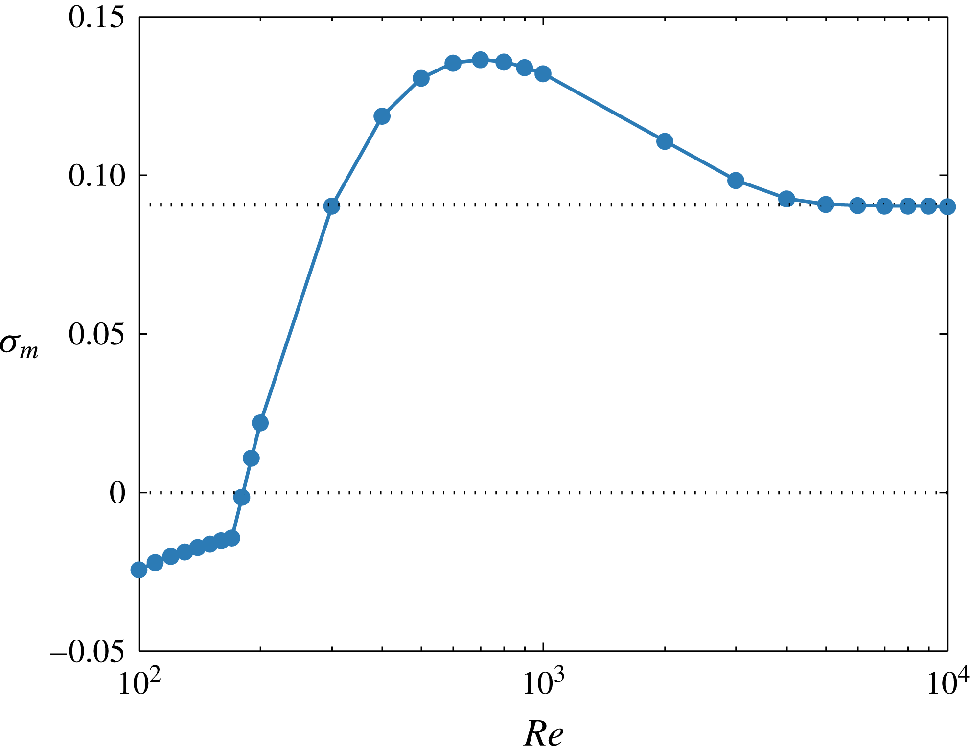
Variation of maximum growth rate
 $\unicode[STIX]{x1D70E}_{m}(Re)$
with
 $Re$
. Dotted lines mark the zero growth rate and the maximum growth rate
 $\unicode[STIX]{x1D70E}_{\infty }=0.0907$
for the inviscid limit with smooth density profiles.

We have solved the linear stability eigenvalue problem for a wide range of Reynolds numbers at this Prandtl number
 $Pr=1$
. In figure 3, we plot against Reynolds number the maximum growth rate over all
 $Ri_{B}$
and
 $\unicode[STIX]{x1D6FC}$
at each Reynolds number, defined as
 $$\begin{eqnarray}\unicode[STIX]{x1D70E}_{m}(Re)=\max _{Ri_{B},\unicode[STIX]{x1D6FC}}[\unicode[STIX]{x1D70E}(Re,Ri_{B},\unicode[STIX]{x1D6FC})].\end{eqnarray}$$
We find that the flow is linearly unstable to two-dimensional normal modes for
 $Re\geqslant 181$
(i.e.
 $\unicode[STIX]{x1D70E}_{m}>0$
for
 $Re\geqslant 181$
), and that
 $\unicode[STIX]{x1D70E}_{m}\rightarrow \unicode[STIX]{x1D70E}_{\infty }=0.0907$
as
 $Re\rightarrow \infty$
. The
 $Re=10\,000$
flow has a very similar maximum growth rate of
 $\unicode[STIX]{x1D70E}_{m}=0.0902$
. However, between these two extremes,
 $\unicode[STIX]{x1D70E}_{m}(Re)$
varies non-monotonically with
 $Re$
, with a global (across
 $Re$
at
 $Pr=1$
) maximum of
 $\unicode[STIX]{x1D70E}_{m}(700)=0.137$
.
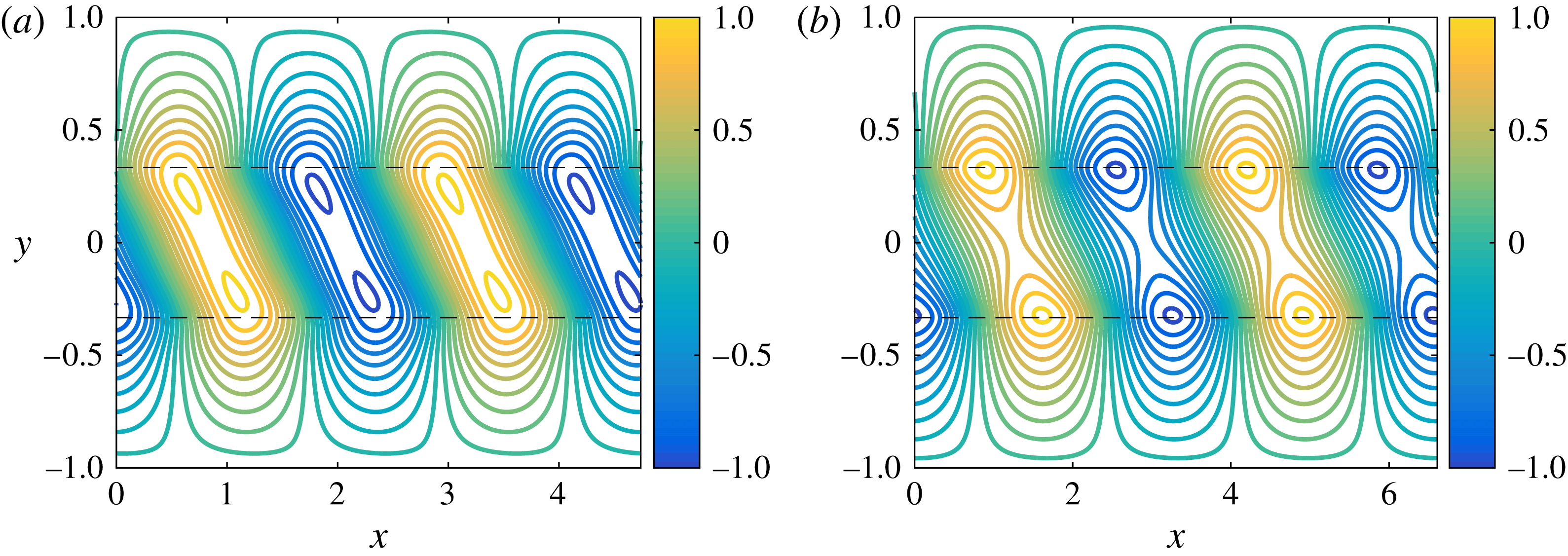
Structure of the vertical velocity for the instability with maximum growth rate
 $\unicode[STIX]{x1D70E}_{m}(Re)$
at
 $Pr=1$
: (a)
 $Re=700$
(with
 $\unicode[STIX]{x1D6FC}=2.65$
); (b)
 $Re=10\,000$
(with
 $\unicode[STIX]{x1D6FC}=1.99$
). Dashed lines show the location of the density interfaces.

Figure 4 shows the structure of the vertical velocity of two wavelengths of the instability with maximum growth rate at both
 $Re=700$
and
 $Re=10\,000$
. In each case the eigenfunction is concentrated about the density interfaces. Unsurprisingly, the eigenfunction is more diffuse for the flow with
 $Re=700$
, apparently allowing a stronger interaction between the two density interfaces, since the eigenfunctions are not so strongly localized at each interface, even though the associated wavenumber
 $\unicode[STIX]{x1D6FC}=2.65$
is somewhat larger than that associated with the flow at
 $Re=10\,000$
,
 $\unicode[STIX]{x1D6FC}=1.99$
. In addition, for a given amplitude, the eigenfunction associated with the
 $Re=700$
flow has stronger gradients, yielding an associated vorticity field with larger maxima and minima.
There is an additional consideration in the linear problem at intermediate
 $Re$
which modifies the spectral properties of the eigenvalue problem at wavenumbers and bulk Richardson numbers close to those associated with the instability with the maximum growth rate
 $\unicode[STIX]{x1D70E}_{m}(Re)$
. In figure 5, we plot contours of growth rate as a function of
 $\unicode[STIX]{x1D6FC}$
and
 $Ri_{B}$
for various
 $Re$
with
 $Pr=1$
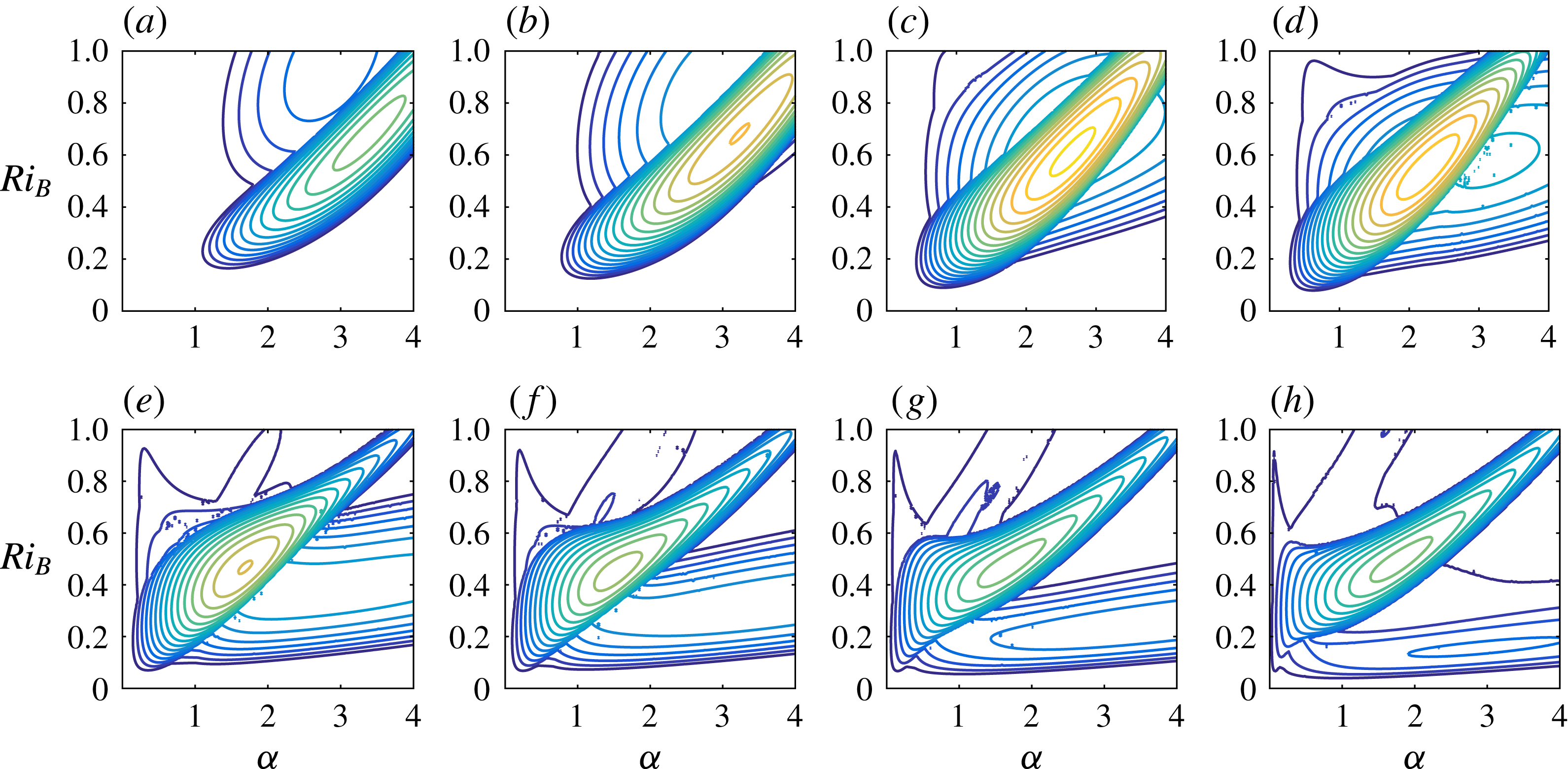
. It is clear that the low-wavenumber instability branch apparent in figure 2(b) shrinks in size as
 $Re$
decreases, and indeed completely disappears for sufficiently small
 $Re$
. As already noted, the growth rates of the globally most unstable TCI vary non-monotonically with Reynolds number, reaching a maximum at
 $Re=700$
. The position, size and shape of the region of the
 $\unicode[STIX]{x1D6FC}{-}Ri_{B}$
plane subject to TCI varies with decreasing Reynolds number. The principal effect of this is that the minimum wavenumber below which the system is stable increases, consistent with the increasingly stabilizing effect of the walls on the largest wavelengths as the Reynolds number is decreased. Nevertheless, in broad terms the unstable TCI branch does not change its location substantially in the
 $\unicode[STIX]{x1D6FC}{-}Ri_{B}$
plane as
 $Re$
varies.
Contours of growth rate of the most unstable instability at
 $Pr=1$
and various values of
 $Re$
: (a)
 $300$
; (b)
 $400$
; (c)
 $700$
; (d)
 $1000$
; (e)
 $2000$
; (f)
 $3000$
; (g)
 $5000$
; (h) 10 000. The central, high-growth-rate branches have zero phase speed and represent TCI. The secondary branches of instabilities have non-zero phase speeds. Contours begin at
 $\unicode[STIX]{x1D70E}=0$
and have 0.008 increments.

On the other hand, as the Reynolds number is varied, the location of the other branch of instability (apparent at low wavenumbers in figure 2
b) does vary significantly in the
 $\unicode[STIX]{x1D6FC}{-}Ri_{B}$
plane. This branch clearly moves towards the region of the unstable TCI branch as the Reynolds number is reduced from 10 000, and the two branches begin to overlap. Indeed, at
 $Re=700$
, which has the global maximum growth rate at
 $Pr=1$
, this unstable branch straddles the unstable TCI branch. As the Reynolds number is reduced further, this other unstable branch emerges at smaller
 $\unicode[STIX]{x1D6FC}$
, or equivalently larger
 $Ri_{B}$
relative to the unstable TCI branch, and the two branches of instability separate once more. At
 $Re=700$
, the most unstable mode over all
 $Ri_{B}$
and
 $\unicode[STIX]{x1D6FC}$
is a TCI occurring at
 $Ri_{B}=0.61$
and
 $\unicode[STIX]{x1D6FC}=2.65$
, with growth rate
 $\unicode[STIX]{x1D70E}_{m}(700)=0.137$
. At these values of
 $Ri_{B}$
and
 $\unicode[STIX]{x1D6FC}$
there is also a pair of instabilities with equal and opposite non-zero real phase speed,
 $c=\pm 0.674$
. It is therefore possible for a primary TCI and another pair of instabilities to be predicted in parallel to be unstable in the same periodic flow domain.
3.3 Dimension of the primary instabilities
Since we observe non-monotonic variation of growth rate of the various instabilities with both
 $Re$
and
 $Ri_{B}$
, it is important to investigate whether three-dimensional modes, with a wavenumber vector oriented at an angle to the mean flow, are actually more unstable than the two-dimensional modes considered above. Squire’s theorem (Squire Reference Squire1933) establishes that the primary linear instability of an unstratified viscous fluid is expected to be two-dimensional at a given Reynolds number
 $Re_{0}$
if
 $$\begin{eqnarray}\left.\frac{\text{d}}{\text{d}s}[Re\unicode[STIX]{x1D70E}_{max}(Re)]\right|_{Re=Re_{0}}>0,\end{eqnarray}$$
where
 $\unicode[STIX]{x1D70E}_{max}$
is the maximum growth rate over
 $\unicode[STIX]{x1D6FC}$
at fixed Reynolds number and
 $\text{d}/\text{d}s$
is the derivative in the direction of increasing Reynolds number along the curve of maximum growth rates. An analogous result due to Yih (Reference Yih1955) establishes that the primary linear instability of an inviscid stratified flow is expected to be two-dimensional at a given bulk Richardson number
 $Ri_{0}$
if
 $$\begin{eqnarray}\left.\frac{\text{d}}{\text{d}s}\left[\frac{\unicode[STIX]{x1D70E}_{max}(Ri_{B})}{Ri_{B}^{1/2}}\right]\right|_{Ri_{B}=Ri_{0}}<0,\end{eqnarray}$$
where now
 $\unicode[STIX]{x1D70E}_{max}(Ri_{0})$
is the maximum growth rate over
 $\unicode[STIX]{x1D6FC}$
at fixed bulk Richardson number, and
 $\text{d}/\text{d}s$
is the derivative in the direction of increasing bulk Richardson number along the curve of maximum growth rates. For the modes considered here, both of the above conditions are satisfied, and so the primary instabilities are expected to be two-dimensional.
4 Nonlinear evolution of the primary instabilities
We conducted several simulations at
 $Pr=1$
,
 $R=30$
for Reynolds numbers in the range
 $500\leqslant Re\leqslant 10\,000$
. In all cases, the two density interfaces diffuse into a state that does not admit a TCI, or indeed the other instabilities with non-zero phase speed, before these primary instabilities reach large enough amplitude to affect the subsequent dynamics of the flow significantly. This is due to the combination of the relatively weak growth rates and the rapid diffusion of such sharp interfaces, even at high
 $Re$
. For this reason, we conducted another linear stability analysis with
 $Pr=300$
. In order for the linear stability code to converge adequately over a reasonable time horizon, we simultaneously reduced the interface sharpness to
 $R=20$
, and this combination of
 $R$
and
 $Pr$
leads to adequate convergence. Typically, we used grids with up to 2048 points in the vertical in our stability code, closely based on that described in Smyth et al. (Reference Smyth, Moum and Nash2011). The variations of the maximum growth rate over all wavenumbers and bulk Richardson numbers,
 $\unicode[STIX]{x1D70E}_{m}(Re)$
, for the case with
 $Pr=300$
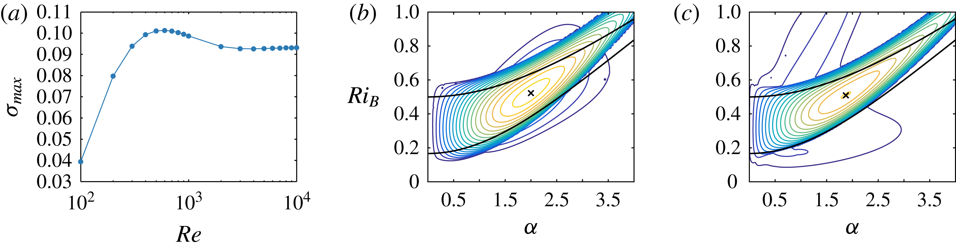
and
 $R=20$
is shown in figure 6(a). We see the same qualitative behaviour as for
 $Pr=1$
, in particular the non-monotonic behaviour with
 $Re$
, but the maximum has shifted to occur for approximately
 $Re=600$
, and the stability threshold for which
 $\unicode[STIX]{x1D70E}_{m}=0$
has moved to
 $Re<100$
.
(a) Maximum growth rate
 $\unicode[STIX]{x1D70E}_{m}(Re)$
at
 $Pr=300$
and
 $R=20$
. (b) Contours of the largest modal growth rate
 $\unicode[STIX]{x1D70E}$
for
 $Re=600$
,
 $Pr=300$
and
 $R=20$
. (c) Contours of the largest modal growth rate
 $\unicode[STIX]{x1D70E}$
for
 $Re=5000$
,
 $Pr=70$
and
 $R=20$
. In both panels (b) and (c), the outermost (and darkest) blue contour has
 $\unicode[STIX]{x1D70E}=0$
, and there is a constant contour interval of
 $0.005$
. The cross marks the values of wavenumber and
 $Ri_{B}$
which are numerically simulated: (b)
 $\unicode[STIX]{x1D6FC}=1.99$
,
 $Ri_{B}=0.52$
, with growth rates
 $\unicode[STIX]{x1D70E}=0.101$
for the TCI and
 $\unicode[STIX]{x1D70E}=0.02$
for the propagating unstable modes (referred to as VHWI) with phase speed
 $c=\pm 0.67$
; and (c)
 $\unicode[STIX]{x1D6FC}=1.87$
,
 $Ri_{B}=0.51$
, with growth rate
 $\unicode[STIX]{x1D70E}=0.093$
for the TCI.

Figure 6(b) shows the largest linear growth rate in the
 $\unicode[STIX]{x1D6FC}{-}Ri_{B}$
plane for
 $Re=600$
with
 $Pr=300$
and
 $R=20$
, and we see again a region of primary TCI overlying another region of primary instability with non-zero real phase speed. The linear stability properties at
 $Pr=300$
and
 $R=20$
are qualitatively the same as for those at
 $Pr=1$
and
 $R=30$
across all Reynolds numbers. We choose to perform a fully nonlinear two-dimensional simulation of the flow at
 $Re=600$
,
 $Pr=300$
and
 $R=20$
. We also want to investigate the dynamics at much higher
 $Re$
, but are unable to do this at
 $Pr=300$
. Instead, we consider
 $Re=5000$
and
 $Pr=70$
. The largest linear growth rate in the
 $\unicode[STIX]{x1D6FC}{-}Ri_{B}$
plane for these parameters is shown in figure 6(c), and the point with maximum growth rate for the TCI does not also have other primary instabilities with non-zero real phase speed. We again see a clear qualitative similarity between the linear stability properties at these parameters as for those with
 $Pr=1$
in the previous section. In particular, by comparison with figure 2(b), there is clear evidence of two other branches of primary instability.
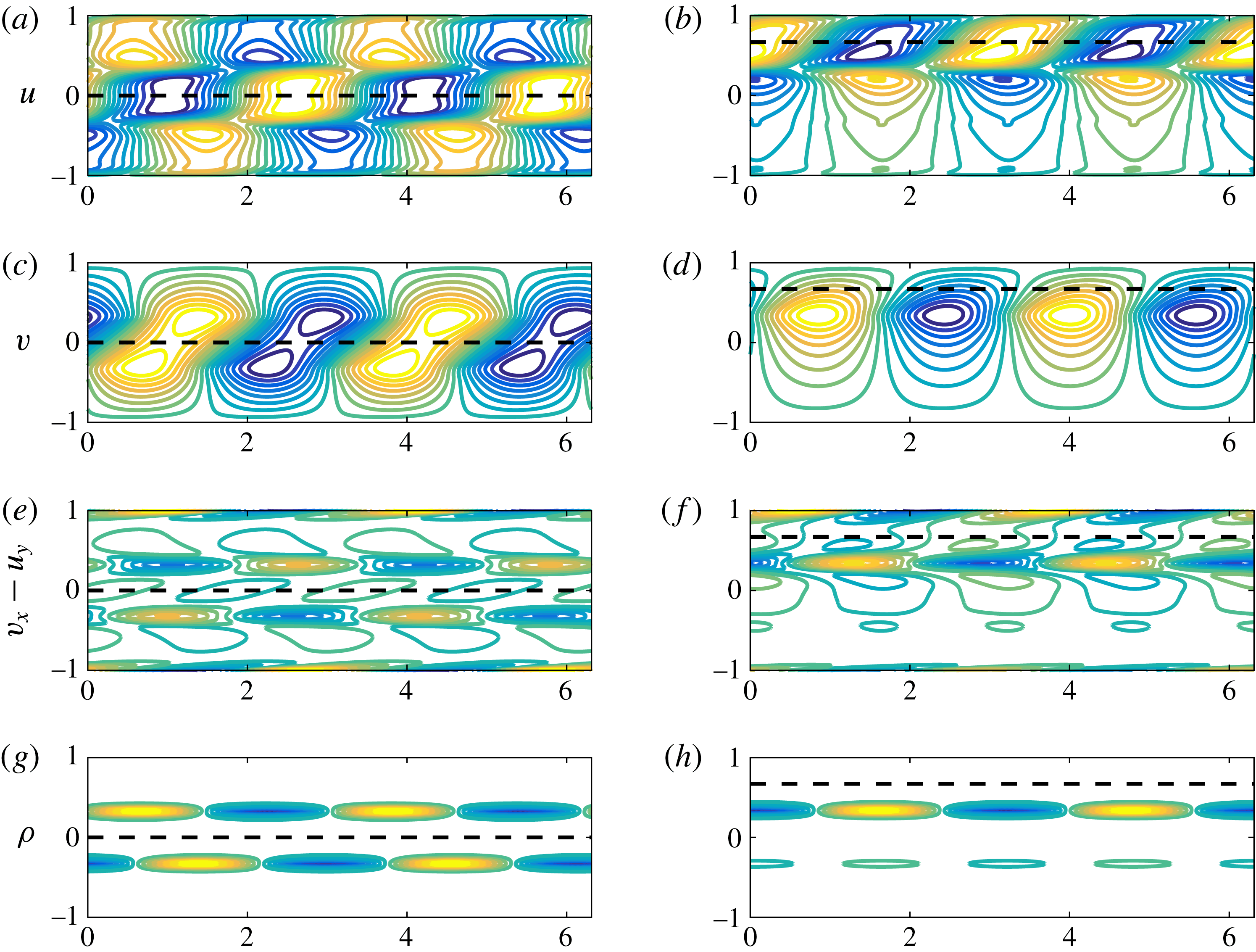
It is clear that these other branches of primary instability only arise at finite Reynolds number, and so it is natural to investigate whether the associated underlying growth mechanisms can be identified. In figure 7, we plot the magnitude of different quantities associated with the eigenfunctions at the parameter values marked with a cross in figure 6(b), i.e.
 $\unicode[STIX]{x1D6FC}=1.99$
,
 $Ri_{B}=0.52$
,
 $Re=600$
,
 $Pr=300$
and
 $R=20$
. For clarity, we show two streamwise wavelengths of the perturbation. In figure 7(a,c,e,g), the structure of the eigenfunction is typical of a TCI (compare for example with figure 2.20 of Sutherland Reference Sutherland2010), with the phase-locked coupling of Doppler-shifted internal waves localized at each of the density interfaces at
 $y=\pm 1/3$
clearly apparent.
Spatial structure of the unstable eigenfunctions in a flow with
 $Re=600$
,
 $Pr=300$
,
 $R=20$
,
 $\unicode[STIX]{x1D6FC}=1.99$
and
 $Re_{B}=0.52$
for the zero real phase speed TCI (a,c,e,g) and the positive real phase speed VHWI (b,d,f,h) showing contours of perturbation: (a,b)
 $u$
; (c,d)
 $v$
; (e,f)
 $\unicode[STIX]{x1D714}$
and (g,h)
 $\unicode[STIX]{x1D70C}$
. Dashed lines mark the height in the flow where the background shear corresponds to the real phase speed of the instability. Note in particular the wall-localized perturbation vorticity for the VHWI in (f). The contour levels are the same as in figure 4.

Figure 7(b,d,f,h) shows the structure of the unstable eigenfunction with non-zero real (and positive) phase speed at these parameter values. (There is another eigenfunction with the same growth rate and structure under the transformation
 $y\rightarrow -y$
.) Panels (f,h), showing the perturbation vorticity distribution and the perturbation density distribution, make it clear that this instability is associated with a strong perturbation at the upper density interface which is phase-locked with the induced perturbation vorticity
 $\unicode[STIX]{x1D714}$
localized at the upper channel wall. (As already discussed, this induced perturbation vorticity localized near the channel wall inherently relies on viscous effects.) The perturbations localized at the density interface are associated with the downstream propagating (i.e. with positive phase speed relative to the local flow speed) internal gravity wave localized at that interface, as is apparent in both the density perturbation and the associated baroclinically induced perturbation vorticity. This internal gravity wave appears to be coupled with the induced localized perturbation vorticity near the horizontal channel wall, which also propagates at the characteristic phase speed of the unstable eigenfunction, and thus behaves analogously to an upstream propagating vorticity wave localized at the edge of a finite-depth shear layer in an inviscid finite-depth shear layer in an unbounded flow. Therefore, we believe that it is appropriate to consider the instability shown in figure 7 as a viscous analogue of the classical HWI, and so we will henceforth refer to this instability as a ‘viscous Holmboe-wave instability’ or VHWI. Indeed, the weaker band of instability at relatively low wavenumber apparent in figure 2(b) can similarly be identified as a viscous analogue of the ‘R’ branch identified in Caulfield (Reference Caulfield1994), associated as it is with an interaction between the vorticity perturbation at one channel wall and the density interface closer to the other channel wall. However, this branch has such small associated growth rates we will not consider it further here.
We have performed two-dimensional, nonlinear numerical integrations of the equations of motion at two sets of parameter values, as identified above. In each case the computational domain is a two-dimensional rectangular channel with no-slip boundary conditions along the (horizontal) channel walls, and periodic boundary conditions at the vertical boundaries of the channel, whose length we denote
 $L_{x}$
. The parameter values we consider in detail here are those marked with crosses in figure 6, although in each case we consider a periodic domain of streamwise length allowing two wavelengths of the primary linear instability (which we thus refer to as a ‘mode-two’ instability) with largest growth rate over all Reynolds numbers and bulk Richardson numbers. Specifically, for
 $Re=600$
and
 $Pr=300$
we have
 $Ri_{B}=0.52$
and
 $L_{x}=6.31$
, corresponding to a TCI with growth rate
 $\unicode[STIX]{x1D70E}_{m}(600)=0.101$
. As discussed above, there is also a primary VHWI with the same wavelength at this
 $Re$
,
 $Pr$
and
 $Ri_{B}$
, with growth rate
 $\unicode[STIX]{x1D70E}=0.020$
. Henceforth, we refer to this simulation as ‘P600’, since it is associated with a primary VHWI. For
 $Re=5000$
and
 $Pr=70$
we have
 $Ri_{B}=0.51$
and
 $L_{x}=6.72$
, which corresponds to two wavelengths of the most unstable primary TCI, with growth rate
 $\unicode[STIX]{x1D70E}_{m}(5000)=0.093$
, and a situation where no primary unstable (either classical or viscous) HWI is compatible with the periodic boundary conditions. We refer to this simulation as ‘S5000’, since any occurrence of HWI in this simulation can only be associated with a secondary instability of a non-trivially modified horizontally averaged flow.
For each of these cases, we study the two-dimensional, nonlinear evolution of both primary and secondary instabilities. It appears that considering a non-dimensional time interval
 $0\leqslant t\leqslant 500$
is sufficient. Although it is well known that primary KHI are susceptible to a wide ‘zoo’ of secondary instabilities, both inherently two-dimensional and three-dimensional (see for example the relatively recent studies of Mashayek & Peltier Reference Mashayek and Peltier2012a
,Reference Mashayek and Peltier
b
) the nonlinear dynamics of layered stratified shear flows with primary TCI has been much less considered, and so it is a natural first step to investigate the two-dimensional nonlinear evolution of such flows.
For such simulations, it is natural to consider the time evolution of the perturbation energy. We consider the perturbation energy density integrated over the whole domain, normalized with respect to both the domain area and the kinetic energy of the initial laminar plane Couette flow, so that the perturbation kinetic energy density
 $K(t)$
, the perturbation potential energy density
 $P(t)$
, and the perturbation total energy density
 $E(t)$
are defined as
 $$\begin{eqnarray}K(t)=\frac{1}{2L_{x}\overline{K}}\int _{0}^{L_{x}}\int _{-1}^{1}\frac{1}{2}\boldsymbol{u}\boldsymbol{\cdot }\boldsymbol{u}\,\text{d}y\,\text{d}x,\end{eqnarray}$$
 $$\begin{eqnarray}P(t)=\frac{1}{2L_{x}\overline{K}}\int _{0}^{L_{x}}\int _{-1}^{1}\frac{Ri_{B}}{2}\unicode[STIX]{x1D70C}^{2}\,\text{d}y\,\text{d}x,\quad E(t)=K(t)+P(t),\end{eqnarray}$$
 $$\begin{eqnarray}\overline{K}=\frac{1}{2L_{x}}\int _{0}^{L_{x}}\int _{-1}^{1}\frac{1}{2}\boldsymbol{U}\boldsymbol{\cdot }\boldsymbol{U}\,\text{d}y\,\text{d}x=\frac{1}{6}.\end{eqnarray}$$
The equations of motion were integrated using Diablo, a parallel Fortran-based Navier–Stokes time-stepping numerical pseudo-spectral code developed by Bewley and Taylor (see Taylor Reference Taylor2008). The code utilizes a Fourier decomposition in the periodic direction, and a finite-difference scheme in the wall-bounded direction with a high-order divergence-free projection multi-step Runge–Kutta–Wray time-stepping scheme which treats viscous terms semi-implicitly using the Crank–Nicholson algorithm, and nonlinear terms explicitly using the momentum-preserving form. The spatial discretization utilizes a staggered grid, which conserves mass, momentum and energy in a discrete sense. We use a
 $2048\times 2033$
grid for both simulations, which is more than sufficient to capture the dynamics down to the Batchelor scale. We initialize both simulations with a small amplitude of the unstable TCI modal form and a smaller-amplitude solenoidal noise field to allow for secondary instabilities. The noise accounts for 1 % by amplitude of the initial condition perturbation. This initialization gives
 $K(0)=P(0)=6\times 10^{-6}$
.
4.1 Simulation P600
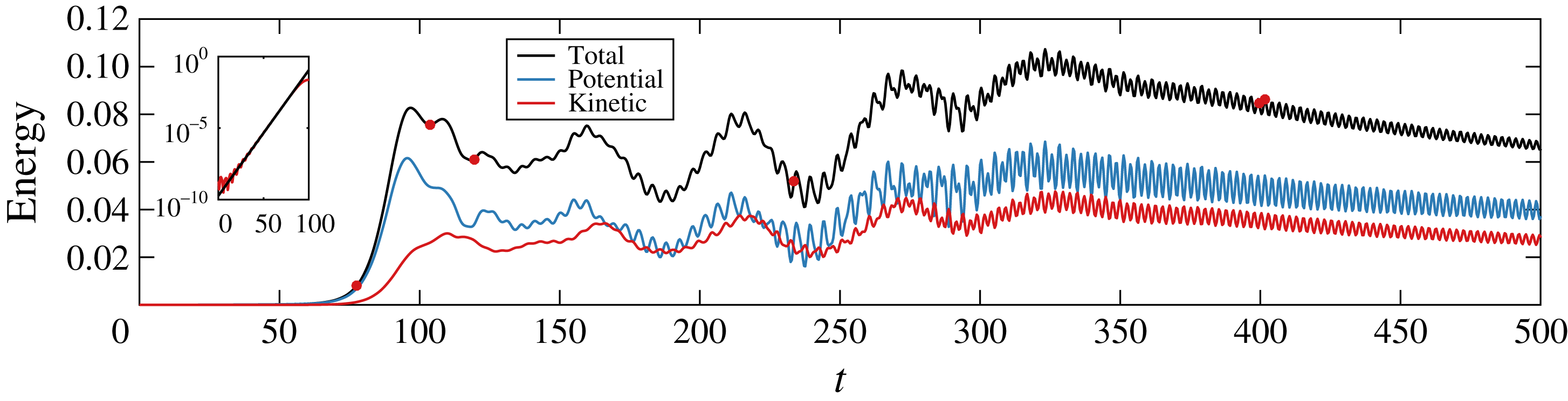
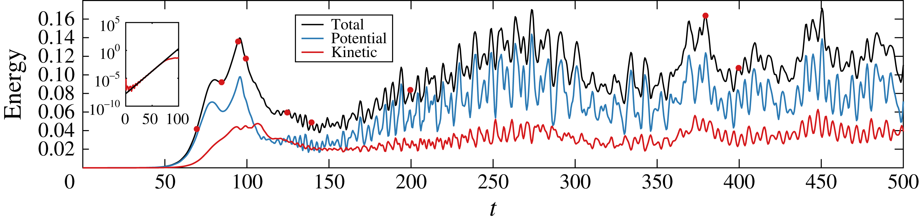
Total energy density (black), kinetic energy density (blue) and potential energy density (red) as a function of time for simulation P600 with
 $Re=600$
,
 $Pr=300$
,
 $Ri_{B}=0.52$
and
 $L_{x}=6.31$
. Red circles mark the times shown in figure 9. Inset: Time evolution of the total energy (red line) compared to the predicted energy growth of the primary TCI (black line).

Figure 8 shows the evolution of the perturbation energy densities from simulation P600 of the flow with
 $Re=600$
,
 $Pr=300$
,
 $Ri_{B}=0.52$
and
 $L_{x}=6.31$
. As is apparent in the inset, the initial energy growth is clearly associated with the linear growth rate of the most unstable TCI. The perturbation energy associated with the TCI reaches a peak amplitude at
 $t\approx 97$
, and subsequently decays whilst slowly oscillating, suggesting strongly that it is not appropriate to describe the TCI as having a ‘saturated’ finite-amplitude manifestation. This behaviour is qualitatively different from the behaviour of flows susceptible to primary KHI, which are known experimentally, numerically and observationally to saturate at finite amplitude as periodic arrays of the classical Kelvin–Helmholtz elliptical ‘billows’.
In this flow, soon after the decay of perturbation energy from its peak value, rapid oscillations appear, as
 $E$
once again increases, reaching a local maximum at
 $t\approx 160$
. This local maximum is followed by a sequence of rapid oscillations of period
 $t_{fast}=4.8\pm 0.1$
. This is very close to the predicted period of oscillation for the primary VHWI of
 $t_{HWI}\approx 4.7$
. During this time the flow is modulated by a slow oscillation of period
 $t_{slow}\approx 56$
until the energy reaches its global maximum around
 $t\approx 320$
, when it then decays at a substantially slower rate. Although the correspondence is not so clear as with the primary TCI, the oscillatory growth of the perturbation energy may be associated with the growth and eventual appearance of the primary VHWI predicted at these parameter values. This suggests that it is indeed possible for qualitatively different primary instabilities to develop in parallel in a stratified shear flow. However, it is important to appreciate that there are undoubtedly profoundly nonlinear dynamics occurring within this flow as well, as for
 $t\gtrsim 270$
the rapid oscillation transitions to another oscillation with a higher frequency, giving a period
 $t_{new}=2.8\pm 0.1$
. The system ultimately settles into this higher-frequency, higher-amplitude oscillation for
 $t\gtrsim 320$
.
Snapshots of the P600 flow evolution at the red circles shown in figure 8 for
 $t=77.6$
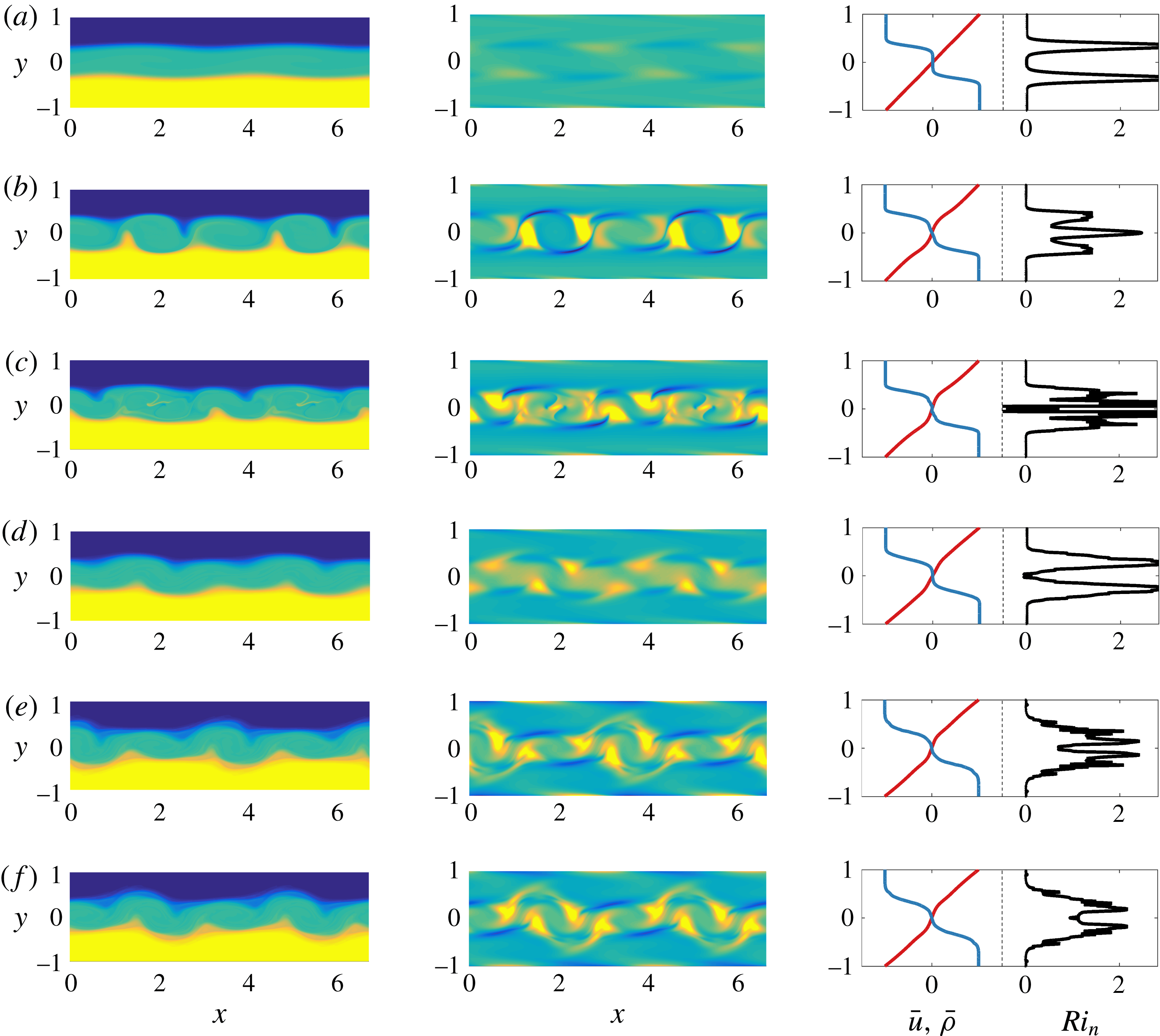
, 103.6, 119.6, 233.6, 399.6, and 401.6 (a–f, respectively). (Left) Total density field, (middle) perturbation vorticity field and (right) mean horizontal velocity (red), mean density (blue) and notional gradient Richardson number (black). Videos of the flow evolution are available as supplementary material.

Figure 9 shows snapshots of the simulation P600 flow at different points during the evolution of the system, enabling us to interpret the observed dynamics of the energy in terms of flow structures. At each time, we plot the total density distribution
 $\unicode[STIX]{x1D70C}_{tot}(x,y,t)$
, (capturing the underlying three-layer structure) and the perturbation vorticity distribution,
 $\unicode[STIX]{x1D714}(x,y,t)$
as defined in (2.8), which is the vorticity in the
 $z$
-direction after the subtraction of the constant (unit in this non-dimensionalization) associated with the laminar background velocity
 $\boldsymbol{U}=y\hat{\boldsymbol{x}}$
. We also plot the streamwise averages of the density distribution
 $\overline{\unicode[STIX]{x1D70C}}(y,t)$
and the streamwise velocity
 $\overline{u}(y,t)$
, where
 $$\begin{eqnarray}\displaystyle \overline{\unicode[STIX]{x1D70C}}(y,t)=\frac{1}{L_{x}}\int _{0}^{L_{x}}\unicode[STIX]{x1D70C}_{tot}\,\text{d}x,\quad \overline{u}(y,t)=\frac{1}{L_{x}}\int _{0}^{L_{x}}u\,\text{d}x. & & \displaystyle\end{eqnarray}$$
In addition, we plot a notional gradient Richardson number
 $Ri_{n}(y,t)$
from these horizontally averaged fields defined as
 $$\begin{eqnarray}\displaystyle Ri_{n}(y,t)=-Ri_{B}\frac{{\displaystyle \frac{\unicode[STIX]{x2202}\overline{\unicode[STIX]{x1D70C}}}{\unicode[STIX]{x2202}y}}}{\left({\displaystyle \frac{\unicode[STIX]{x2202}\overline{u}}{\unicode[STIX]{x2202}y}}\right)^{2}}, & & \displaystyle\end{eqnarray}$$
which proves to be a useful measure for the extent to which nonlinear processes modify the linear stability properties of the flow. In particular, snapshots of
 $Ri_{n}(y,t)$
allow us to identify whether the fundamental three-layer structure of the flow subject to a larger scale, close to linear shear, persists or is substantially modified by nonlinear processes. Videos of the flow evolution are available as supplementary material at https://doi.org/10.1017/jfm.2016.686.
At early times, as is apparent in figure 9(a), the two density interfaces form inward-facing (i.e. towards the midpoint of the flow) cusps and are drawn towards each other at these points. This is typical of the nonlinear manifestation of the TCI observed experimentally by Caulfield et al. (Reference Caulfield, Peltier, Yoshida and Ohtani1995) and the previous two-dimensional numerical simulations of Lee & Caulfield (Reference Lee and Caulfield2001). These cusps are naturally induced by the (positive) vorticity redistributing into elliptical vortices, spanning the entire depth of the middle layer, a characteristic finite-amplitude manifestation of the TCI. However, the induced cusps also lead to baroclinic vorticity generation, which is strongly negative at the interfaces’ cusps. Unlike the KHI at finite amplitude, it is clear from figure 9(b,c) that the TCI consists of a coupled vortical structure, with a central (positive) vortical core flanked by two negative vortical wings. We also see in figure 9(b) that four vortical cores have formed from the mode-two primary TCI, and in 9(c) that two of these cores have grown to have larger streamwise extent than the other two cores. The formation of an extra pair of vortical cores is due to the attempted pinching together of the cusps on opposite density interfaces becoming misaligned due to the background shear, and so inducing two extra cusps on each interface.
The vortical cores appear to be tilted into the base shear, and thus have the potential to extract energy from the base flow transiently through the Orr mechanism (Orr Reference Orr1907). However, this tilting also induces modifications of the density field, leading to annihilation of the different-signed vorticity distributions, and hence the primary TCI instability is almost entirely sheared out by the background flow, as is apparent in figure 9(d). The shearing out process has also lessened the extent of the asymmetry between the alternating large and small streamwise extent of the vortical cores. Indeed, the spatial periodicity of the primary TCI is typically rapidly destroyed by the secondary instabilities, and the mode-two primary TCI is only briefly apparent within the flow.
It is apparent in figure 9(d), showing the horizontally averaged density and velocity profiles and the associated notional gradient Richardson number
 $Ri_{n}(y,t)$
, that the growth (and decay) of the primary TCI does not modify the base flow qualitatively, in that there remains a clear bimodal peak in the Richardson number, associated with a smooth variation of velocity across the entire flow, with two relatively ‘sharp’ interfaces persisting to separate three close-to-constant density layers.
During shearing out of the remnants of the nonlinear evolution of the TCI, mode-two Holmboe waves appear above the upper density interface and below the lower density interface. We believe that these waves are the eventual nonlinear appearance of the primary VHWI present in the original flow profile, which has a substantially smaller growth rate
 $\unicode[STIX]{x1D70E}_{HWI}(600)=0.020$
than the primary TCI which has growth rate
 $\unicode[STIX]{x1D70E}_{m}(600)=0.101$
. As already noted, the observed period of oscillation of the perturbation energy is close to the predicted period of oscillation of this primary VHWI. Furthermore, as is apparent in the perturbation vorticity field, particularly in the video available as supplementary material, the appearance of this instability is closely correlated with the appearance of propagating vorticity perturbations localized near the channel walls. It is important to appreciate that we do not initialize the flow with the modal form of this instability, but rather only with the modal form of the primary TCI and small-amplitude noise. Due to the combination of this different initialization, and the relative growth rates of the two primary instabilities, it is unsurprising that this primary instability reaches finite amplitude substantially later than the TCI.
Before the vortices are sheared out fully, the primary VHWI has grown sufficiently to produce large-amplitude nonlinear Holmboe waves which travel along the density interfaces. These nonlinear Holmboe waves prevent the vortices from developing any subsequent streamwise asymmetry, and they remain approximately equally spaced throughout the remaining evolution. The nonlinear Holmboe waves reach a peak total energy at
 $t\approx 320$
, before slowly decaying. The characteristic feature of a (one-sided) nonlinear Holmboe wave is a patch of vorticity (in this case with positive sign) above the density interface that pulls wisps of fluid from the layer on the other side of the interface into the layer where the vorticity patch is. In this system, the nonlinear Holmboe waves that propagate consist of two wavelengths (i.e. they are ‘mode-two’ instabilities), and there are two patches of vorticity at each interface, as can be seen in figure 9(e,f). These patches grow in intensity and size over time, interacting with the perturbation vorticity localized near to each of the channel walls. Indeed this nonlinear interaction appears to mediate the continued growth of the nonlinear Holmboe waves and initiates the slow decay for
 $t\gtrsim 320$
, and is specific to PCF at finite
 $Re$
due to the non-slip boundary condition at the channel walls.
It is clear that a primary (albeit inherently viscous) HWI of the initial base flow has grown in ‘parallel’ to the primary TCI, even though its growth rate is appreciably smaller. Therefore, as hypothesized in Caulfield et al. (Reference Caulfield, Peltier, Yoshida and Ohtani1995), it is possible for multiple primary instabilities to grow to finite amplitude in layered stratified shear flows, with different growth rates and phase speeds (and hence critical layer locations). Furthermore, here the HWI is apparently more robust than the TCI, calling into question the conventional assumption that the most unstable mode of linear theory will continue to dominate at finite amplitude as
 $t\rightarrow \infty$
.
4.2 Simulation S5000
Total energy density (black), kinetic energy density (blue) and potential energy density (red) as a function of time for the simulation with
 $Re=5000$
and
 $Pr=70$
. Red circles mark the times shown in figure 11. Inset: Time evolution of the total energy (red line) compared to the predicted energy growth of the primary TCI (black line).

Snapshots of the S5000 flow evolution at the red circles shown in figure 10 for
 $t=70$
, 85, 95, 100, 125, 140, 200, 380 and 400 (a–i, respectively). (Left) Total density, (middle) perturbation vorticity field and (right) mean horizontal velocity (red), mean density (blue) and notional gradient Richardson number (black). Videos of the flow evolution are available as supplementary material.

Turning our attention to the higher-Reynolds-number flow, figure 10 shows the evolution of the perturbation energy densities from simulation S5000 for the flow with
 $Re=5000$
,
 $Pr=70$
,
 $Ri_{B}=0.51$
and
 $L_{x}=6.72$
. There is a clear first peak in energy at
 $t\approx 80$
that results from the growth of the most unstable normal mode, and it is followed by another peak in energy at
 $t\approx 95$
. After this second maximum, the energy subsequently decays rapidly. There is then an onset of ‘fast’ oscillations, and the energy recovers until a maximum at
 $t\approx 275$
, setting into a slower oscillation for
 $t\gtrsim 150$
. After
 $t\approx 275$
, the flow transitions into a yet slower oscillation coupled with an appreciably longer time-scale nonlinear modulation. This behaviour continues for
 $t\gtrsim 300$
and is reminiscent of the energetics of the nonlinear Holmboe wave state found by Balmforth et al. (Reference Balmforth, Roy and Caulfield2012). Figure 11 shows snapshots of the flow at different points during the evolution of the system, which we now discuss in detail. Videos of the flow evolution are available as supplementary material.
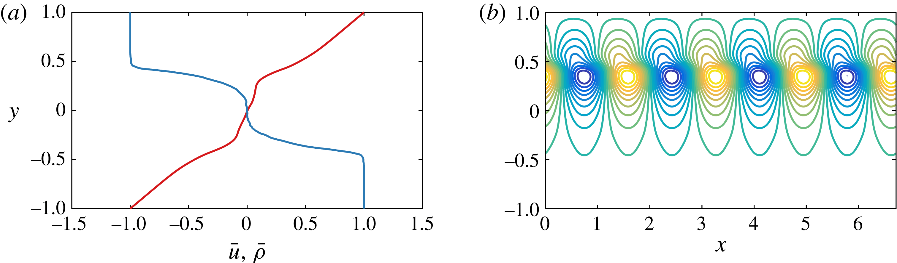
(a) Detail of the mean horizontal velocity (red) and mean density (blue) at
 $t=125$
, taken from figure 11(e). (b) Vertical velocity
 $v$
for a most unstable mode of these mean profiles.

As in the lower-Reynolds-number flow simulation P600 discussed above, the evolution of the unstable linear TCI results in cusps and streaks of vorticity forming on the density interfaces, pulling them towards each other, as can be seen in figure 11(a). These vorticity streaks then begin to roll up to form two coherent vortical cores, i.e. a primary mode-two instability develops. Similarly to the lower-Reynolds-number flow, the vortical cores begin to lose energy as they are sheared out. However, as the vortices are sheared out, there is once more a misalignment of the cusps on the density interfaces, resulting in the creation of two more vortical cores located between the primary pair of vortical cores, as is evident in figure 11(b). The two newly created vortical cores begin to grow in size, and appear to squeeze the two original vortical cores. This causes complex spatio-temporal vorticity dynamics within the two original vortical cores, as is evident in figure 11(c,d). The squeezing of the two original vortical cores causes a cascade of secondary braid-like instabilities that results in small-scale disorder in the intermediate layer, and a destruction of the cusps on the two density interfaces due to vigorous mixing in the intermediate layer. The disordered vorticity field is evident in figure 11(e).
The mean velocity profile during this disordered state exhibits increased shear over the laminar profile at each of the two density interfaces, as can be clearly seen in figure 12(a), where we show a detailed version of the horizontal mean profiles
 $\overline{u}$
and
 $\overline{\unicode[STIX]{x1D70C}}$
found in figure 11(e). This increased shear spontaneously creates eight regions of negative vorticity, four above the upper density interface and four below the lower density interface, as seen in figure 11(f). These vortices also pull wisps of fluid from the intermediate density layer into both the upper and lower density layers, and are clearly associated with the parasitic appearance of a nonlinear Holmboe wave. This HWI is categorically not a primary instability for this flow at this wavelength, and so the appearance of a parasitic nonlinear Holmboe wave has occurred in ‘series’ to the nonlinear development and subsequent decay of the primary TCI. Furthermore, this secondary HWI is of ‘classical’ type, associated with the localized intensified shear in the vicinity of each density interface clearly seen in figure 12, and not the perturbation vorticity localized near the channel walls. The vigorous mixing associated with the braid-instability-driven decay of the evolution of the primary TCI has rearranged the mean fields in just such a way as to cause the flow to become susceptible to the appearance of HWI. Indeed, a linear stability analysis of a nominal flow corresponding to the horizontally averaged mean profiles shown in figure 12(a) predicts unstable HWI modes with both positive and negative phase speed, and wavelength corresponding to 25 % of the horizontal extent of the computational domain. One of these mode-four modes (with positive phase speed) is plotted in figure 12(b). This prediction is consistent with the nonlinear structures which are observed to develop subsequently, although there is of course no a priori reason why the stability properties of the horizontally averaged total flow should correspond precisely to observations when the actual real flow exhibits non-trivial spatial and temporal variability. Soon after the appearance of mode-four nonlinear Holmboe waves there is a coarsening to mode-two nonlinear Holmboe waves, as is apparent from the two vortices above the upper density interface and two vortices below the lower density interface in figure 11(g).
The mode-two nonlinear Holmboe wave state gradually increases in energy during
 $150\lesssim t\lesssim 275$
. As for the P600 simulation discussed above, the peak in energy at
 $t\approx 275$
appears to correspond with the mode-two state interacting with the flow boundaries, and this mediates the end of continued energy growth. As the flow begins to decay, there is yet another coarsening event, and the flow settles onto a large-amplitude mode-one (i.e. with the same wavelength as the streamwise length of the entire computational domain) nonlinear Holmboe wave for
 $t\gtrsim 350$
. This final state, which is visible in figure 11(h,i), is reminiscent of the large-amplitude nonlinear Holmboe wave found by Balmforth et al. (Reference Balmforth, Roy and Caulfield2012), and its appearance is associated with parasitic development on the remnants of the evolution of the primary TCI.
Although such two-dimensional simulations at high Reynolds number should be treated with caution, two key conclusions consistent with the results of Balmforth et al. (Reference Balmforth, Roy and Caulfield2012) can be drawn. First, the TCI is clearly ‘fragile’ and prone to strong secondary two-dimensional instabilities at high Reynolds number. Second, those secondary instabilities can modify the base flow in a way that then leads to the ‘parasitic’ development of HWI in ‘series’ at later times in layered stratified shear flows. This is apparently due to the local intensification of shear at each of the relatively sharp density interfaces, as is apparent in figure 12.
5 Discussion
Layered stratified shear flow typically admits a number of linear instabilities, namely a stratified version of the well-known Kelvin–Helmholtz instability (KHI) (Helmholtz Reference Helmholtz1868; Kelvin 1871) and also the inherently stratified Holmboe wave instability (HWI) (Holmboe Reference Holmboe1962) and the so-called Taylor–Caulfield instability (TCI) (Taylor Reference Taylor1931). We considered the linear modal stability of three-layer stratified plane Couette flow that does not have an inflection point in the velocity field to exclude by construction the KHI and to focus only on inherently stratified instabilities. The analysis of Caulfield (Reference Caulfield1994), the experiments of Caulfield et al. (Reference Caulfield, Peltier, Yoshida and Ohtani1995), the numerical simulation of Lee & Caulfield (Reference Lee and Caulfield2001) and the asymptotic stratified defect theory of Balmforth et al. (Reference Balmforth, Roy and Caulfield2012) suggest that this flow is unstable to primary TCI as well as a viscous analogue of the classical HWI, depending on the various parameters in the problem. We refer to this inherently viscous instability, which relies fundamentally on localized perturbation vorticity near to the channel walls due to the no-slip boundary condition, as a VHWI.
The linear stability analysis presented here shows that these flows are susceptible to primary instabilities of both TCI type and VHWI type, and that the TCI is the most unstable linear mode for both an idealized inviscid, non-diffusive stepped three-layer density profile (for which the VHWI cannot occur) and also over a range of Reynolds numbers for a viscous, diffusive hyperbolic tangent smoothed three-layer density profile. The viscous, diffusive, smooth density profile is subject to VHWI with smaller growth rates (at least for this depth of intermediate layer) than the primary TCI, and the streamwise wavenumbers and bulk Richardson numbers for which the TCI and VHWI occur varies with the Reynolds number. In particular, there are parameters for which both the TCI and VHWI are unstable, and for which only the TCI is unstable. For Prandtl number
 $Pr=1$
and
 $Pr=300$
the largest growth rate over all streamwise wavenumbers and bulk Richardson numbers is a non-monotonic function of the Reynolds number; nevertheless, theorems due to Squire (Reference Squire1933) and Yih (Reference Yih1955) demonstrate that the primary instability is expected to be two-dimensional.
The numerical calculations of Lee & Caulfield (Reference Lee and Caulfield2001) and Balmforth et al. (Reference Balmforth, Roy and Caulfield2012) indicated that the nonlinear evolution of the TCI is dominated by the secondary appearance of finite-amplitude Holmboe waves, and indicates that this could occur either in parallel due to the existence of a primary HWI or in series due to a nonlinear modification of the initial flow fields that is conducive to the appearance of Holmboe waves. (In the finite-
 $Re$
PCF considered here, the only possible primary HWI is of VHWI type.) In order to investigate this more fully, we performed fully nonlinear two-dimensional evolutions of the Boussinesq Navier–Stokes equations in the plane Couette flow geometry for two cases, one corresponding to two wavelengths of both primary TCI and VHWI, and another corresponding to two wavelengths of only primary TCI. We found that, for small Prandtl numbers, such as
 $Pr=1$
, the density interfaces diffuse more rapidly than the TCI can grow to significant amplitude. Therefore, we considered two simulations. In the simulation referred to as simulation P600, with
 $Re=600$
and
 $Pr=300$
, the flow is susceptible to both a primary TCI and VHWI, while in the simulation referred to as S5000, with
 $Re=5000$
and
 $Pr=70$
, there is only a primary TCI.
For simulation P600, for which there is both a primary TCI and VHWI, the faster growing TCI grows to large amplitude before decaying, and does not saturate. During the decay of the nonlinear evolution of the primary TCI, we see clear evidence of the nonlinear manifestation of the primary VHWI, having apparently grown in parallel to the primary TCI. The subsequent dynamics of the flow are inherently linked to the nonlinear Holmboe waves that appear from the primary VHWI, and the nonlinear evolution of the primary TCI only sets the scale of the four equally sized elliptical vortical cores, a scale which is not predicted to be linearly unstable, that reside in the intermediate density layer, around which the nonlinear Holmboe waves propagate.
For simulation S5000, for which there is only a primary TCI, the primary TCI once more grows to large amplitude before rapidly decaying. This nonlinear evolution once again forms four vortical cores, two large ones from the primary TCI and two secondary vortical cores. The two secondary vortical cores rapidly increase in size so that the two primary vortical cores are squeezed. This squeezing causes a cascade of braid instabilities, and causes the entire intermediate density layer to become disordered. The mean properties of this newly created disordered state, which is the remains of the nonlinear evolution of the primary TCI, appears susceptible to the appearance of (classical) HWI. Mode-four nonlinear Holmboe waves appear rapidly in the flow, which undergo a coarsening to a mode-one nonlinear Holmboe wave due to the presence of the flow boundaries. This mode-one nonlinear Holmboe wave persists for the remainder of the flow evolution we simulate, and is strongly reminiscent of the coarsening HWI found by Balmforth et al. (Reference Balmforth, Roy and Caulfield2012). It appears that nonlinear Holmboe waves grow parasitically, in series to the TCI on the nonlinearly modified flow fields, even when there is no primary HWI. For both cases the TCI proves to be very fragile at finite amplitude, whereas HWI appear to be very robust in such two-dimensional flows.
We have demonstrated that in layered sheared flow, which is susceptible to both primary TCI and HWI, the nonlinear evolution of the TCI does not ‘saturate’ at finite amplitude, but instead the dynamics are dominated by the secondary appearance of either the primary HWI, if it exists, or of parasitic secondary nonlinear Holmboe wave dynamics even in the absence of a primary HWI. The nonlinear evolution of the TCI inevitably occurs alongside nonlinear Holmboe waves, consistent with the observations of Balmforth et al. (Reference Balmforth, Roy and Caulfield2012). This is to be contrasted with the traditional view of the nonlinear evolution of primary linear instabilities like the KHI, for which the nonlinear evolution saturates at finite amplitude, and is relatively robust in the sense that the primary billows survive for some time.
The investigation of the nonlinear evolution of primary TCI has been relatively neglected in comparison to that of primary KHI and HWI, and so although it is well known that such instabilities are subject to a ‘zoo’ of secondary instabilities, particularly in three dimensions (Mashayek & Peltier Reference Mashayek and Peltier2012a ,Reference Mashayek and Peltier b ; Mashayek et al. Reference Mashayek, Caulfield and Peltier2013), an initial restriction to two-dimensional dynamics is warranted in this layered flow. Even for two-dimensional dynamics, we have identified a rich array of secondary processes associated with the appearance of nonlinear Holmboe waves as both the Reynolds number and Prandtl number are varied. We believe that a three-dimensional investigation of the nonlinear evolution of primary TCI is called for in order to understand better the dynamics of layered stratified shear flows, in particular to investigate whether the fragility of the TCI and the robustness of the HWI persist in flows which are free to evolve in three dimensions.
Acknowledgements
Thanks are due to two anonymous referees, whose thoughtful and constructive comments have substantially improved this paper. T.S.E. is supported by a SIMS studentship. A preliminary version of this research was presented at Euromech Colloquium 547 – Trends in Open Shear Flow Instability, which was held in honour of Patrick Huerre’s 65th birthday. C.P.C. would like to acknowledge Professor Huerre for his support and encouragement over many years, and this article is dedicated to him with heartfelt thanks. The research activity of C.P.C. is supported by EPSRC Programme Grant EP/K034529/1 entitled ‘Mathematical Underpinnings of Stratified Turbulence’. Data used to create figures 1–8, 10 and 12, and the initial condition header data for Diablo for the two key simulations P600 and S5000, are available at https://doi.org/10.17863/CAM.6144.
Supplementary movies
Supplementary movies are available at https://doi.org/10.1017/jfm.2016.686.