1. Introduction
Printing functional materials for organic electronics applications or biological inks in tissue engineering is an intricate challenge as the printing techniques must often be adapted to the material properties. These properties can be complex, with fluids ranging from Newtonian to viscoplastic and viscoelastic. Many printing techniques rely on physical contact between the ink and a blade, a nozzle or a pattern (Deblais et al. Reference Deblais, Harich, Colin and Kellay2016; Yan et al. Reference Yan, Dong, Su, Han, Song, Wei and Shi2018; Glasser, Alizée, Eric & Georges Reference Glasser, Cloutet, Hadziioannou and Kellay2019; Zhou, Fu & He Reference Zhou, Fu and He2020). Contact between the fluid and the solid surfaces of the printing device can cause clogging or degradation of the material through substantial shear or extension. These modifications can be desirable for certain printing techniques. Shear thinning is useful for inkjet printing and the presence of a yield stress is useful for blade coating. Nevertheless, the high sensitivity of printing processes to both fluid and mechanical properties narrows the utility of each method. A robust and flexible technique which avoids such drawbacks is laser-induced forward transfer (LIFT) (Bohandy, Kim & Adrian Reference Bohandy, Kim and Adrian1986). A submerged bubble is nucleated near a liquid–gas interface by a laser-induced plasma, whose subsequent dynamics produces liquid jets accomplishing material transportation and deposition. As it is contactless and nozzle free, LIFT can be adapted to different materials from Newtonian or complex liquids to biological materials for printing, dispensing controlled amounts of fluid, or producing jets with very high velocities intended for hypodermic injections (Mézel et al. Reference Mézel, Souquet, Hallo and Guillemot2010; Gruene et al. Reference Gruene, Unger, Koch, Deiwick and Chichkov2011; Brown et al. Reference Brown, Brasz, Ventikos and Arnold2012; Tagawa et al. Reference Tagawa, Oudalov, Visser, Peters, van der Meer, Sun, Prosperetti and Lohse2012; Yan et al. Reference Yan, Huang, Xu and Chrisey2012; Ali et al. Reference Ali, Pages, Ducom, Fontaine and Guillemot2014; Zhang et al. Reference Zhang, Xiong, Mei, Huang and Chrisey2015; Desrus et al. Reference Desrus, Chassagne, Moizan, Devillard, Petit, Kling and Catros2016; Petit et al. Reference Petit, Kérourédan, Devillard and Cormier2017; Turkoz, Deike & Arnold Reference Turkoz, Deike and Arnold2017; Turkoz et al. Reference Turkoz, Perazzo, Kim, Stone and Arnold2018; Jalaal et al. Reference Jalaal, Schaarsberg, Visser and Lohse2019b). This technique is used in two configurations. The first configuration requires the presence of a sacrificial film, such as a metallic film, which is heated (and damaged) by the laser light to produce an expanding bubble and eventually liquid jets (Gruene et al. Reference Gruene, Unger, Koch, Deiwick and Chichkov2011; Brown et al. Reference Brown, Brasz, Ventikos and Arnold2012; Yan et al. Reference Yan, Huang, Xu and Chrisey2012; Ali et al. Reference Ali, Pages, Ducom, Fontaine and Guillemot2014; Zhang et al. Reference Zhang, Xiong, Mei, Huang and Chrisey2015; Turkoz et al. Reference Turkoz, Deike and Arnold2017, Reference Turkoz, Perazzo, Kim, Stone and Arnold2018). In the second configuration, investigated here, the laser is focused directly in the bulk of a fluid layer just beneath the liquid–air interface (Patrascioiu et al. Reference Patrascioiu, Fernández-Pradas, Palla-Papavlu, Morenza and Serra2014b; Desrus et al. Reference Desrus, Chassagne, Moizan, Devillard, Petit, Kling and Catros2016; Petit et al. Reference Petit, Kérourédan, Devillard and Cormier2017; Jalaal et al. Reference Jalaal, Schaarsberg, Visser and Lohse2019b). This configuration is attractive for applications including bio-printing as it minimizes the presence of impurities engendered by the eventual degradation of a sacrificial film.
An obstacle of both LIFT configurations is the complex phenomenology of the jet formation, with most reports showing that this occurs in two stages (Patrascioiu et al. Reference Patrascioiu, Fernández-Pradas, Palla-Papavlu, Morenza and Serra2014b; Petit et al. Reference Petit, Kérourédan, Devillard and Cormier2017; Jalaal et al. Reference Jalaal, Schaarsberg, Visser and Lohse2019b). The first stage produces very thin ( $\sim$10
 $\mathrm {\mu }$m) and fast (
 $\sim$10 m s
 $^{-1}$) jets. In the second stage, a relatively thick (
 $\sim$100
 $\mathrm {\mu }$m) and slow (
 $\sim$1 m s
 $^{-1}$) jet is produced. The first jet can be utilized for high resolution printing if the comparatively thicker second jet is avoided. However, the first jet is too thin to be suitable for printing functional materials such as suspensions of large particles or bio-materials such as cells, which the second jet is potentially capable of. If properly understood, this complexity can be exploited to provide a versatile printing method.
The fluid mechanics of the interaction between an oscillating bubble and a free surface has been studied for some time (Pearson et al. Reference Pearson, Cox, Blake and Otto2004; Lauterborn & Kurz Reference Lauterborn and Kurz2010), with military applications of underwater explosions providing an early motivation to understand this phenomenon (Davies & Taylor Reference Davies and Taylor1942). Observations and analyses of principally the first jet in laboratory-scale experiments have steadily provided new insights into the bubble dynamics and first jet formation, aided by improved technology and numerical simulations (Chahine Reference Chahine1977; Chahine & Bovis Reference Chahine and Bovis1980; Blake & Gibson Reference Blake and Gibson1987; Robinson et al. Reference Robinson, Blake, Kodama, Shima and Tomita2001; Patrascioiu et al. Reference Patrascioiu, Fernández-Pradas, Palla-Papavlu, Morenza and Serra2014b). There appears to be broad consensus that the first jet is engendered by the impulse of the initial expansion of the bubble after initiation (Patrascioiu et al. Reference Patrascioiu, Fernández-Pradas, Morenza and Serra2014a). In particular, there is good overall agreement between experiments and theoretical calculations which employ the Kelvin impulse (Blake & Gibson Reference Blake and Gibson1987). And more recent analysis using a boundary integral formulation can quantitatively reproduce the detailed features of the first jet and even its counter-jet (Pearson et al. Reference Pearson, Cox, Blake and Otto2004). The dynamics of and mechanism behind the second jet formation, on the other hand, is comparatively less studied and understood.
Although the second jet itself has not been as extensively studied, there are numerous studies that, while focusing on the first jet, also investigated the formation of a crown that can follow the emergence of the first jet (Kiyama et al. Reference Kiyama, Tagawa, Ando and Kameda2016; Koukouvinis et al. Reference Koukouvinis, Gavaises, Supponen and Farhat2016; Liu et al. Reference Liu, Cui, Ren and Zhang2017; Li et al. Reference Li, Zhang, Wang, Li and Liu2019). The formation of the crown and the formation of the second jet appear to be intricately linked. Although some have argued that compressibility effects such as large pressure waves are responsible for the crown (Kiyama et al. Reference Kiyama, Tagawa, Ando and Kameda2016), explicitly incompressible simulations (Liu et al. Reference Liu, Cui, Ren and Zhang2017) that reproduce the crown demonstrate that compressibility is not essential to the phenomenon. Moreover the effects of the shock produced by the bubble nucleation last for only a few microseconds after bubble nucleation (Jalaal et al. Reference Jalaal, Li, Klein Schaarsberg, Qin and Lohse2019a), well before the formation of the second jet, and a recent parametric study of the crown formation concluded that the shock wave impinging on the surface is not responsible for the crown (Saade et al. Reference Saade, Jalaal, Prosperetti and Lohse2021).
Here, by carrying out a comprehensive experimental and numerical study, we clarify the mechanism behind the formation of the second jet and elucidate both its properties and the conditions for its emergence. We demonstrate that the mechanism behind the second jet formation is unique and unlike the mechanism behind the first jet formation. In particular, the origin of the second jet is the secondary flow generated by the bubble dynamics. The paper is organized as follows. In § 2, we provide information regarding the experimental set-up and the numerical methods. In § 3, we present our initial experimental and numerical results, showing the broad agreement between these two approaches. In § 4 we elucidate the mechanism behind the formation of the second jet and use this to formulate a scaling argument to understand the dependence of the second jet velocity on parameters such as initial bubble depth and pressure. Finally, in § 5 we summarize our findings.
2. Experimental and numerical methods
Our experimental set-up consists of an amplified titanium–sapphire femtosecond laser emitting at 800 nm with a pulse duration of 65 fs, pulse energy of 3 mJ and a repetition rate of 1 kHz. A Pockels cell, synchronized with the laser, selects a smaller repetition rate going from a fraction of a Hz to several Hz. The laser beam, of typical radius 2 mm, is then focused with a long working distance microscope objective (50 $\times$ N.A. 0.5 (Olympus SLMPLN series)) in a volume of liquid (ultrapure water from a Millipore/Milli Q system) contained in a rectangular fused quartz cell (Hellma 101.150
 $\phi$s) with a square transparent base of 1 cm
 $^2$. The pulse energy can be varied using a half-wave plate combined with a polarizing beamsplitter from 2.5 to 30
 $\mathrm {\mu }$J. The objective was mounted on a stage for a precise positioning of the focal point with respect to the liquid–air interface. The laser beam waist was estimated to be roughly 1
 $\mathrm {\mu }$m. The cell walls were rendered hydrophobic using OTS (octadecyltrisiloxane) in Toluene solution to minimize the effect of the meniscus on the visualization. A high speed camera (Phantom V 640) equipped with a magnifying lens (Navitar) was then used to visualize the dynamics of both bubble and jet formation. Typical frame rates were 110 000 frames s
 $^{-1}$ with an exposure time of 1
 $\mathrm {\mu }$s. The spatial resolution was 3.5
 $\mathrm {\mu }$m pix
 $^{-1}$. The acquisition of the images from the camera was triggered using a train of pulses delivered by an Agilent generator, itself synchronized to a recurring starting pulse powered by the Pockels cell driver.
For the numerical simulations, we use the open-source package OpenFOAM (Jasak, Jemcov & Tukovic Reference Jasak, Jemcov and Tukovic2007), a finite-volume solver for partial differential equations, such as the Navier–Stokes equations. For the time integration we use an Euler scheme with the time step dynamically set to ensure a maximum Courant number less than 0.25. We use compressibleInterFOAM, a solver for two compressible, non-isothermal immiscible fluids, which uses a volume of fluid method to solve for the volume fraction of the liquid phase  $\gamma$ with the transport equation (Miller et al. Reference Miller, Jasak, Boger, Paterson and Nedungadi2013; Koch et al. Reference Koch, Lechner, Reuter, Köhler, Mettin and Lauterborn2016; Zeng, Gonzalez-Avila & Ohl Reference Zeng, Gonzalez-Avila and Ohl2020)
 \begin{align} \frac{\partial \gamma}{\partial t} + \boldsymbol{\nabla} \boldsymbol{\cdot} (\gamma \boldsymbol{u}) + \boldsymbol{\nabla} \boldsymbol{\cdot} (\gamma (1 - \gamma) \boldsymbol{U}_{\boldsymbol{r}} &= \gamma (1-\gamma) \left( \frac{1}{\rho_g}\frac{{\rm D} \rho_g}{{\rm D} p_g} - \frac{1}{\rho_l}\frac{{\rm D} \rho_l}{{\rm D} p_l} \right) \frac{{\rm D} p}{{\rm D}t}\nonumber\\ &\quad + \gamma \boldsymbol{\nabla} \boldsymbol{\cdot} \boldsymbol{u}, \end{align}
where  $\boldsymbol {u}$ is the velocity field,
 $\boldsymbol{U}_{\boldsymbol{r}}$ is the relative velocity between the two phases,
 $t$ is time,
 $p$ is the pressure,
 $\rho$ is the density and the subscripts
 $g$ and
 $l$ represent the gas and liquid phases, respectively. The final term on the left-hand side is an artificial term that counteracts the numerical diffusion of the interface, keeping it sharp (Rusche Reference Rusche2003; Koch et al. Reference Koch, Lechner, Reuter, Köhler, Mettin and Lauterborn2016). The compressibilities
 ${\rm D} \rho / {\rm D} p$ are determined by the equation of state for the gas and liquid phases, which for simplicity we choose to be the ideal gas and fluid laws, neglecting higher-order effects of temperature and pressure (Miller et al. Reference Miller, Jasak, Boger, Paterson and Nedungadi2013; Koch et al. Reference Koch, Lechner, Reuter, Köhler, Mettin and Lauterborn2016). Numerical simulations using compressibleInterFOAM have recently been performed to study cavitation and jetting in thin gaps (Zeng et al. Reference Zeng, Gonzalez-Avila and Ohl2020).
Heat and mass transfer are neglected, and the governing equations for the motion of the fluid are then the continuity equation
 \begin{equation} \frac{\partial \rho}{\partial t} + \boldsymbol{\nabla} \boldsymbol{\cdot} (\rho \boldsymbol{u} ) = 0, \end{equation}
and the compressible Navier–Stokes equations
 \begin{equation} \frac{\partial \rho \boldsymbol{u}}{\partial t} + \boldsymbol{\nabla} \boldsymbol{\cdot} (\rho \boldsymbol{u} \boldsymbol{u}) ={-} \boldsymbol{\nabla} p + \boldsymbol{\nabla} \boldsymbol{\cdot} \tau + \boldsymbol{F}, \end{equation}
where  $\tau$ is the viscous stress tensor
 $\tau = \mu [ \boldsymbol {\nabla } \boldsymbol {u} + \boldsymbol {\nabla } \boldsymbol {u}^T - \frac {2}{3} (\boldsymbol {\nabla } \boldsymbol {\cdot } \boldsymbol {u}) \boldsymbol{\mathsf{I}}]$, with
 $\mu$ the dynamic viscosity and
 $\boldsymbol{\mathsf{I}}$ the identity tensor;
 $F$ is the force due to surface tension which is modelled using a continuous-surface-force method which preserves the sharpness of the interface in order to accurately estimate the curvature (Brackbill, Kothe & Zemach Reference Brackbill, Kothe and Zemach1992; Koch et al. Reference Koch, Lechner, Reuter, Köhler, Mettin and Lauterborn2016).
Equations (2.1)–(2.3) are solved together in a rectilinear domain. The extent of the three-dimensional (3-D) simulation domain was 400  $\mathrm {\mu }$m in both horizontal directions (
 $x$,
 $y$) and ranged from 800 to 1200
 $\mathrm {\mu }$m in the vertical direction (
 $z$), with the liquid–air interface (
 $z=0$) fixed at 300
 $\mathrm {\mu }$m above the domain bottom. We used a uniform resolution of
 ${{\rm d} x} = 2$
 $\mathrm {\mu }$m. The boundary conditions are zero gradient at all domain boundaries. More information on the sensitivity to domain size and resolution can be found in Appendix A.
Simulating the exact experimental situation, including the laser–fluid interaction, is complex. To simplify our approach, we assume that this interaction simply nucleates a small bubble of initial high pressure  $P$ beneath the surface at
 $z = -H$ (
 $x = y = 0$). We use a spherical bubble with initial radius
 $R_0 = 10$
 $\mathrm {\mu }$m, which remains roughly spherical during the initial dynamics. This is significantly different from experiments where the bubbles observed experimentally are elongated in the direction of the beam (the focal area is a vertically elongated ellipsoid due to the necessarily weak numerical aperture of the long working distance objective). As we show, despite these simplifications, our numerical simulations capture the essential features of the experimental observations.
3. Results
In experiments we vary both the focal point depth  $H$ below the interface as well as the pulse energy
 $E$. The typical phenomenology of the jet formation following bubble nucleation for a fixed
 $E$ and
 $H = 144$
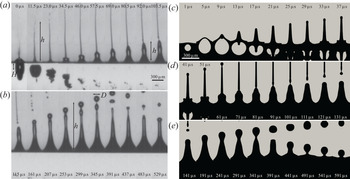
 $\mathrm {\mu }$m is shown in figure 1. After nucleation, the bubble rapidly expands, reaches a maximum size then contracts and recoils away from the interface. Notwithstanding the presence of the interface and substantial asymmetry, the bubble dynamics is in fair agreement with the predicted behaviour of the Rayleigh–Plesset equation (Vogel et al. Reference Vogel, Noack, Nahen, Theisen, Busch, Parlitz, Hammer, Noojin, Rockwell and Birngruber1999; Lauterborn & Kurz Reference Lauterborn and Kurz2010) (see Appendix B). The initial bubble expansion correlates with the formation of the first rapid jet. As this thin jet rises, the bubble deflates and recoils into the bulk fluid. Moments later (
 $t \sim 30$
 $\mathrm {\mu }$s) a second bulge emerges from the interface and the slower, thicker second jet emerges as in previous observations (Patrascioiu et al. Reference Patrascioiu, Fernández-Pradas, Palla-Papavlu, Morenza and Serra2014b). During the emergence of this second jet the bubble has deflated completely as it recoils away from the interface. While the first jet disintegrates into a train of rapidly rising drops (of size
 $\sim$20
 $\mathrm {\mu }$m) the second jet becomes unstable at the tip and engenders drops of much larger size (
 $D \sim 100$
 $\mathrm {\mu }$m).
(a,b) Sequence of side-view images illustrating the experimental bubble and jet dynamics, the nucleation depth  $H$, the jet height
 $h$ and the droplet diameter
 $D$. The laser pulse energy is
 $E = 18.3$
 $\mathrm {\mu }$J and
 $H = 144$
 $\mathrm {\mu }$m. The first thin jet appears concomitantly with the bubble expansion while the second jet emerges
 $\sim$30
 $\mathrm {\mu }$s later when the bubble has deflated and recoiled away from the interface. (c–e) Numerical analogue of the experimental images. Vertical slices (
 $y$–
 $z$ plane) of the 3-D numerical simulations of the bubble and jet dynamics. Here,
 $H = 80$
 $\mathrm {\mu }$m and the initial bubble pressure is
 $P = 600$ bars. The second jet is beginning to emerge
 $\sim$30
 $\mathrm {\mu }$s after initiation. The simulations reproduce the main features of the experiments and show additional details such as the counter-jet (
 $t = 17$
 $\mathrm {\mu }$s) not easily observed in our experiments.

The first jet, now well understood, is produced by the impulse of the initial bubble expansion. Previous work has suggested that the mechanism for the second jet is the same (Patrascioiu et al. Reference Patrascioiu, Fernández-Pradas, Palla-Papavlu, Morenza and Serra2014b), with the second jet corresponding to the second bubble expansion. To investigate this in more detail, we have carried out a numerical study which provides information not available in experiments and reveals the detailed velocity and pressure fields responsible for the second jet formation. As with experiments, we systematically vary  $H$ and
 $P$, which replaces
 $E$, to uncover their significance for the jet's behaviour.
To estimate appropriate values of  $P$ to correspond with experiments is not a simple task as only a fraction of the pulse energy is transformed into bubble energy (Vogel et al. Reference Vogel, Noack, Nahen, Theisen, Busch, Parlitz, Hammer, Noojin, Rockwell and Birngruber1999). Following Fabbro et al. (Reference Fabbro, Fournier, Ballard, Devaux and Virmont1990) and Jalaal et al. (Reference Jalaal, Schaarsberg, Visser and Lohse2019b), a characteristic pressure due to the laser pulse can be estimated using
 \begin{equation} P_c = (\alpha(I-I_{th}))^{1/2} (\rho c)^{1/2}, \end{equation}
where  $I$ is the laser intensity,
 $I_{th}$ is the plasma threshold intensity,
 $\rho = 1000$ kg m
 $^{-3}$ is the density of water,
 $c = 1500$ m s
 $^{-1}$ is the speed of sound in water and
 $\alpha$ (
 $\simeq$0.01) is the small fraction of the laser energy that finally contributes to the bubble energy (Vogel et al. Reference Vogel, Noack, Nahen, Theisen, Busch, Parlitz, Hammer, Noojin, Rockwell and Birngruber1999). With an estimated laser spot radius of
 $\sim$1
 $\mathrm {\mu }$m, an energy of
 $E \sim 1$
 $\mathrm {\mu }$J and a plasma threshold of
 $I_{th} \simeq 6\times 10^{16}$ W m
 $^{-2}$ (Linz et al. Reference Linz, Freidank, Liang and Vogel2016), we estimate a characteristic pressure of
 $P_c \sim 3\times 10^6$ bars, which, although large, is of a similar order of magnitude to estimates in similar experiments (Schaffer et al. Reference Schaffer, Nishimura, Glezer, Kim and Mazur2002). We confirm this estimate by comparing the oscillations of a bubble nucleated far from the interface with the predictions of the Rayleigh–Plesset equation (see Appendix B). This comparison suggests a similar order of magnitude for the pressure for an initial bubble radius
 $R_0 \sim 1$
 $\mathrm {\mu }$m, a scale too small to resolve in our finite spatial resolution simulations. An important parameter, as we will see below, is the bubble energy
 $\sim P R_0^3$. Keeping this constant we thus increase the initial radius to
 $R_0 = 10$
 $\mathrm {\mu }$m and explore initial pressures
 $10^2 \lesssim P \lesssim 10^3$ bars. Figure 1 shows a sequence of images of the bubble and jetting dynamics from simulations that are remarkably similar to experiments. A first and second jet, droplet formation and the bubble oscillations are all observed, as well as a counter-jet not easily observable in our experiments (Patrascioiu et al. Reference Patrascioiu, Fernández-Pradas, Palla-Papavlu, Morenza and Serra2014b).
We further compare the experimental and numerical results by studying the dynamics of jet formation for different values of  $H$,
 $E$ (for experiments) and
 $P$ (for simulations). In this work we focus on
 $H \gg R_0$ to avoid bubble bursting (Sanjay, Lohse & Jalaal Reference Sanjay, Lohse and Jalaal2021). In figure 2 we plot the heights
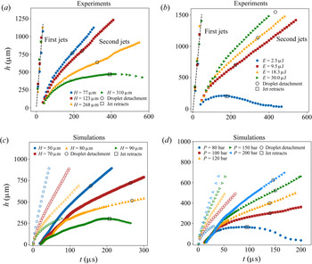
 $h$ of the first and second jets as a function of time, giving a quantitative picture of the phenomenology just described. At early times
 $h$ corresponds to the jet tip, while at later times it corresponds to the furthest point of the released droplet, if any (see figure 1). For experiments, in figure 2(a) we systematically vary
 $H$ for fix
 $E = 18.3$
 $\mathrm {\mu }$J, while in figure 2(b) we systematically vary
 $E$ for relatively fixed
 $H \simeq 144$
 $\mathrm {\mu }$m. Within our precision the velocity of the first jet
 $U_1$ is hardly affected by varying
 $H$ or
 $E$. The velocity
 $U_2$ of the second jet, on the other hand, is strongly affected by both
 $H$ and
 $E$. The second jet first decelerates before reaching a steady velocity,
 $U_2$, until it becomes unstable to a Rayleigh–Plateau-like instability engendering droplets with velocities close to that of the rising jet. The open circles in figure 2(a,b) indicate the position of drop formation. For fixed
 $E = 18.3$
 $\mathrm {\mu }$J (figure 2a)
 $U_2$ is a decreasing function of
 $H$ until a threshold value of
 $H = H_c \simeq 300$
 $\mathrm {\mu }$m, below which the jet retracts and no droplets are shed. Likewise for a fixed value of
 $H \simeq 144$
 $\mathrm {\mu }$m (figure 2b)
 $U_2$ shows a systematic dependence on
 $E$ with a threshold below which no jets can be produced (Vogel et al. Reference Vogel, Noack, Nahen, Theisen, Busch, Parlitz, Hammer, Noojin, Rockwell and Birngruber1999). The diameter
 $D$ of the shed droplets, however, depends only weakly on
 $H$ and
 $E$ (see figure 2a). The sensitivity of
 $U_2$ to
 $H$ and
 $E$ suggests that it can be tuned to affect how droplets impact a surface for printing (Zhang et al. Reference Zhang, Xiong, Corr and Huang2016). In figure 2(c) we show the jet time series for different values of
 $H$ for fixed
 $P = 400$ bar, while in figure 2(d) we show the same for different values of
 $P$ with fixed
 $H = 40$
 $\mathrm {\mu }$m. The time series from the simulations are both qualitatively and quantitatively similar to the experiments. The second jet emergence time (
 $\sim$20
 $\mathrm {\mu }$s), the droplet detachment time (
 $\sim$200
 $\mathrm {\mu }$s) and the first jet velocity (
 $\sim$30 m s
 $^{-1}$), and second jet velocity (
 $\sim$3 m s
 $^{-1}$) are all quantitatively similar for simulations and experiments. Likewise, the dependence of second jet velocity
 $U_2$ and drop diameter
 $D$ on
 $H$ and
 $P$ mimic the experimental behaviour with
 $D$ being less sensitive than
 $U_2$ (see Appendix C). A notable difference between experiments and simulations is the significant dependence of
 $U_1$ on
 $H$ and
 $P$ in simulations (see figure 2c,d), although our experiments may simply have insufficient temporal resolution to see a similar dependence.
(a) Experimental jet height  $h$ vs time
 $t$ for
 $E = 18.3$
 $\mathrm {\mu }$J and varying
 $H$. For large
 $H$ no drop formation occurs at the tip of the second jet which simply retracts. (b) Experimental
 $h$ vs time
 $t$ for different energies
 $E$ and
 $H \simeq 120$
 $\mathrm {\mu }$m. (c) Value of
 $h$ vs time from numerical simulations for different
 $H$ and fixed initial pressure
 $P = 400$ bar. The first jet is indicated by open symbols. (d) Same as (c) for different initial pressures
 $P$ and fixed
 $H = 40$
 $\mathrm {\mu }$m. The open circles indicate the time at which drop detachment occurs. The data after this time indicate the position of the drop vs time. The drops travel at basically the same velocity as the jet in this regime of approximately constant velocity. The open squares indicate the retraction time.

4. Analysis and discussion
While there exists detailed analysis and theory for the initial jet formation due to the expanding bubble (Blake & Gibson Reference Blake and Gibson1987; Robinson et al. Reference Robinson, Blake, Kodama, Shima and Tomita2001), there appears to be little understanding of the second, thicker jet. Previous work has argued that the mechanism for the second jet differs little from that of the first jet (Patrascioiu et al. Reference Patrascioiu, Fernández-Pradas, Palla-Papavlu, Morenza and Serra2014b): the secondary bubble expansion pushes the fluid away from the free surface into the air. However, in both experiments and simulations, the second jet emerges when the bubble is imploding and recoiling away from the interface, before it has begun its second expansion (as in figure 1 for  $t \lesssim 25$
 $\mathrm {\mu }$s and figure 5a). If the second jet were the product of the second bubble expansion, then one would expect a delay even longer than the several microseconds between the first bubble expansion and first jet (see figure 1c) since the bubble is even further from the surface when the second jet emerges. The absence of any delay points to the failure of the argument that the second jet arises from the second expansion.
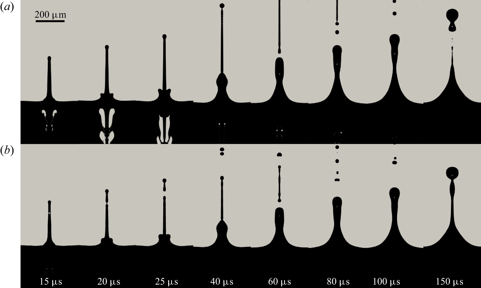
A qualitative test of the hypothesis of the importance of the secondary expansion for the second jet can be made by artificially removing the bubble when it reaches its minimum size in a simulation (see figure 3). When the bubble reaches its minimum size at  $t \simeq$ 14
 $\mathrm {\mu }$s, after its implosion, we set the phase in the submerged bubble to water, leaving the velocity, pressure and temperature fields as they are. In this way the second expansion is effectively, albeit artificially, removed. A comparison between a simulation with (figure 3a) and without (figure 3b) the second expansion shows only minute differences. The second jet still emerges and engenders a large droplet. If the second expansion is not responsible for the second jet, its source must be sought elsewhere.
Vertical slices of the simulations at different times for  $P = 200$ bars and
 $H = 40$
 $\mathrm {\mu }$m. The liquid (water) phase is dark and the gas (air) phase is light. Until time
 $t \simeq 14$
 $\mathrm {\mu }$s, when the bubble size reaches its first minimum, the two simulations (a) and (b) are the same with dynamics as in figure 1 for
 $t \lesssim 25$
 $\mathrm {\mu }$s. Then for (b), the bubble is artificially removed by setting the air phase below the interface to water and the simulation allowed to evolve. In this way the second expansion of the bubble is removed. A comparison of the second jet with (a) and without (b) the second expansion shows that the second jet is much the same in its absence.

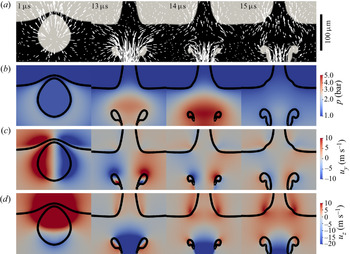
Here, the additional information provided by the simulations becomes essential. In figure 4 we show the velocity and pressure fields of a representative simulation where  $P = 200$ bar and
 $H = 40$
 $\mathrm {\mu }$m. These fields are consistent with the explanation that the first jet is created by the initial bubble expansion pushing the fluid upward, the primary flow. The pressure gradient is directed radially away from the bubble, and the velocity is likewise directed radially outward. During the initial formation of the second jet, however, the velocity and pressure fields are significantly different. The pressure is much larger below the surface than at the surface, and the largest gradient occurs when the bubble is at its minimum size (
 $t=14$
 $\mathrm {\mu }$s). The collapse of the bubble, which becomes toroidal, generates a rapidly retracting counter-jet and a substantial inflow into the region between the bubble and the surface (
 $t = 13$
 $\mathrm {\mu }$s). This creates the high-pressure region below the surface as well as a saddle flow (
 $t = 14$
 $\mathrm {\mu }$s). The lateral flow into the region between the bubble and the surface, which we term the secondary flow and which is established before the bubble expansion, appears to be the source of the second jet. Less than 1
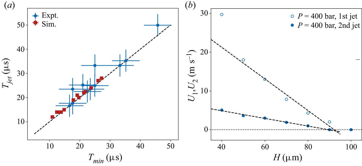
 $\mathrm {\mu }$s later, the second jet has already emerged, well before the bubble re-expands. In figure 5(a) we show the time of the second jet emergence
 $T_{jet}$ vs the time that the bubble collapses to its minimum size
 $T_{min}$. The near perfect correlation between the two times for all pressures, energies and depths reinforces our argument that the second jet is related to the bubble contraction, and the secondary flow it engenders, and not the bubble re-expansion. Identifying the secondary flow as the mechanism behind the second jet formation, as done qualitatively in Chen et al. (Reference Chen, Yu, Su, Chen and Chen2013), permits a simple analysis of the second jet velocity scaling.
Vertical slices of the simulated flow fields at  $t = 1$, 13, 14 and 15
 $\mathrm {\mu }$s for
 $P = 200$ bars and
 $H = 40$
 $\mathrm {\mu }$m, focusing on the region near the interface. (a) Plots of the liquid (dark) and air (light) phases with velocity vectors super-imposed. The velocity vector lengths at
 $t = 1$
 $\mathrm {\mu }$s correspond to the distance a fluid particle will travel in 1
 $\mathrm {\mu }$s, while the velocity vector lengths for the remaining times correspond to the distance a fluid particle will travel in 2
 $\mathrm {\mu }$s. (b) Colour plots of the pressure field
 $p$. The phase boundaries are indicated by thick black lines. (c) Colour plots of the horizontal velocity
 $u_y$. (d) Colour plots of the vertical velocity
 $u_z$. The first column (
 $t = 1$
 $\mathrm {\mu }$s) shows the bubble several
 $\mathrm {\mu }$s prior to the emergence of the first jet. The remaining columns are before (
 $t = 13$
 $\mathrm {\mu }$s), during (
 $t = 14$
 $\mathrm {\mu }$s) and after (
 $t = 15$
 $\mathrm {\mu }$s), the emergence of the second jet, which is accompanied by a substantial secondary flow. A substantial secondary flow accompanies the emergence of the second jet, with the flow drawn in by the bubble collapse and counter-jet feeding the second jet and creating the large pressure gradient that drives it.

(a) Plot of the second jet emergence time  $T_{jet}$ vs the time when the submerged bubble reaches its minimum size
 $T_{min}$. The uncertainties on the experimental and numerical results correspond to the time between recorded times, 9 and 1
 $\mathrm {\mu }$s, respectively. (b) Plot of the first
 $U_1$ and second
 $U_2$ jet velocity vs
 $H$ for fixed
 $P = 400$ bar from simulations. Both vary approximately linearly near a threshold value of
 $H_c \simeq 90$
 $\mathrm {\mu }$m.

Mass conservation determines a relationship between the secondary inflow velocity and the second jet velocity,  $U_2$. Although the degree of contribution to the secondary flow from the bubble collapse and counter-jet is unclear, we attribute the large downward flow in figure 4(a) (
 $t \geq 13$
 $\mathrm {\mu }$s) to the counter-jet, which we assume has a velocity comparable to the first jet
 $U_1$. By considering a cylindrical volume of liquid of diameter
 $D_c$ and length
 $l_c$, we can write
 $2 {\rm \pi}(D_c/2) l_c U \sim {\rm \pi}(D_c/2)^2 U_1$, which yields
 \begin{equation} U \sim U_1 \frac{D_c}{4 l_c}. \end{equation}
We anticipate that  $D_c$ corresponds to the maximum nucleated bubble size
 $D_{max}$ while the vertical length scale
 $l_c$ is as yet unknown. (Additional evidence for a single horizontal length scale proportional to
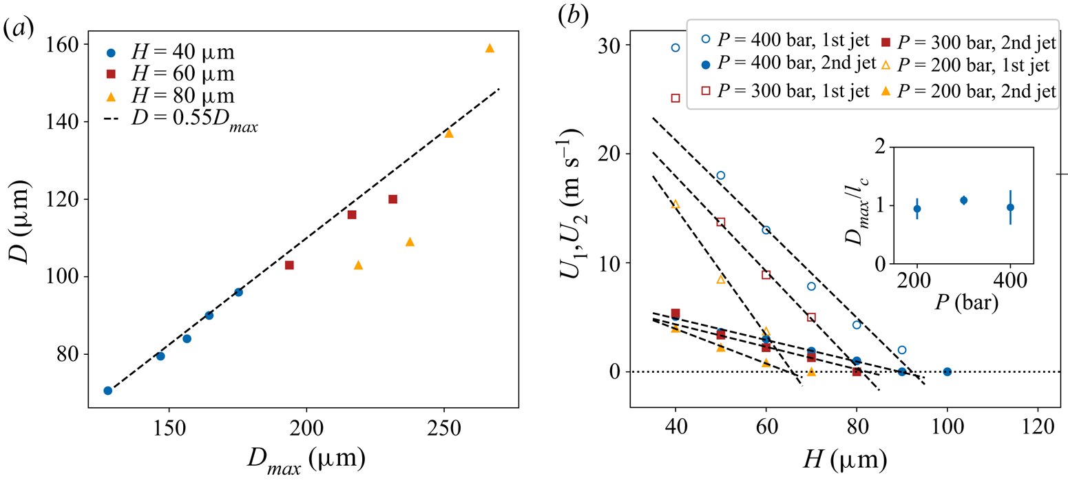
 $D_{max}$ is given in figure 6(a), where we show that the droplet diameter
 $D \propto D_{max}$.) In figure 5(b) we plot both
 $U_1$ and
 $U_2$ vs
 $H$ for simulations at
 $P = 400$ bar. Both velocities decrease approximately linearly with
 $H$ and approach zero at
 $H \sim 90$
 $\mathrm {\mu }$m, beyond which no jetting is observed. The ratio between
 $U_2$ and
 $U_1$ is thus constant and given by
 $D_{max}/4 l_c$ (4.1), which after measuring
 $D_{max}$ yields
 $l_c$. In figure 6(b) we show that
 $l_c \simeq D_{max}$ for several values of
 $P$. The bubble dimensions thus set the relation between
 $U_2$ and
 $U_1$.
(a) Plot of the droplet size  $D$ vs horizontal maximum bubble diameter
 $D_{max}^h$ from simulations. Combining the results from several depths indicates that
 $D \propto D_{max}^h$. (b) Plot of first
 $U_1$ and second
 $U$ jet velocity vs initial depth
 $H$ from simulations for three different initial pressures
 $P = 200$, 300 and 400 bar. For all pressures, both
 $U_1$ and
 $U$ decrease nearly linearly to zero at a critical depth
 $H^*$. The ratio of the slopes of these two lines is
 $D_{max}/4l_c$, as argued in the main text. Inset:
 $D_{max}/l_c$ vs
 $P$. The ratio is close to unity for all
 $P$, suggesting that there is only a single dominant length scale.

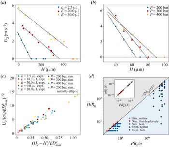
In figure 7(a,b) we show that the linearity of  $U_2$ with
 $H$ up to a threshold value
 $H_c$, as in figure 5(b), is generic for both experiments with fixed
 $E$ and for additional simulations with fixed
 $P$. Unsurprisingly, the critical depth
 $H_c$ increases while the slope
 $\partial U / \partial H$ decreases with an increase of
 $E$ or
 $P$. The similarities between these graphs suggest that the experimental and numerical results can be brought into correspondence with a suitable normalization. Since we have argued that the second jet is associated with bubble collapse, we estimate a characteristic bubble collapse velocity as
 $U_{\sigma } = \sqrt {\sigma /\rho D_{max}}$, where
 $\sigma$ is the surface tension between water and air, and normalize
 $U_2$ with
 $U_\sigma$. To account for the dependence on a critical depth
 $H_c$, we plot
 $U_2/U_\sigma$ vs
 $(H_c - H)/D_{max}$, which is similar to but distinct from the standoff distance
 $2H/D_{max}$ used in previous work (Pearson et al. Reference Pearson, Cox, Blake and Otto2004) by virtue of the inclusion of
 $H_c$ necessary for collapse. As figure 7(c) shows, the data collapse satisfactorily. Although the bubbles in the simulations are roughly spherical, the bubbles in experiments are strongly elliptical, so to account for this asymmetry we used the maximum bubble horizontal width
 $D^h_{max}$ and vertical length
 $D^v_{max}$ as the relevant length scales. In the simulations these two length scales are nearly the same. If different, as in experiments, we expect the vertical length scale
 $D^v_{max}$ to affect the critical depth
 $H_c$, while we expect the horizontal length
 $D^h_{max}$ to control the bubble collapse speed. Thus
 $D^v_{max}$ is used to normalize
 $(H_c - H)$ and
 $D^h_{max}$ is used to normalize the velocity. With these choices the experiments and simulations collapse, but separately. To bring them into accord with each other, we introduce a parameter
 $\beta \simeq 0.48$ which is used only for the simulations to artificially modify the length scales
 $D^v_{max}$ and
 $D^h_{max}$. Since the value of
 $\beta$ is close to the ratio of the
 $D^h_{max}$/
 $D^v_{max}$ for experiments (see Appendix B), this suggests that we have fully captured the behaviour of both simulations and experiments with the normalization in figure 7(c), excepting a dependence on the bubble asymmetry at its maximum size.
The second jet velocity  $U_2$ vs initial depth
 $H$ for (a) experiments with several fixed
 $E$ and (b) simulations with several fixed
 $P$. All curves reveal the same linearity of
 $U_2$ with
 $H$ and a threshold
 $H_c$. (c) Second jet velocity
 $U_2$ from experiments and simulations normalized by
 $U_\sigma = (\sigma /\rho \beta D_{max}^h)^{1/2}$ vs a normalized distance from the interface
 $(H_c-H)/\beta D_{max}^v$. Here,
 $\beta = 0.48$ (close to the experimental ratio
 $D_{max}^h/D_{max}^v \simeq 0.41$) brings the experiments into accord with the simulations, including initially simulations where the initial bubble shape was elliptic (see Appendix D). (d) Phase diagram for jetting using the two normalized control parameters
 $H/R_0$ and
 $PR_0/\sigma$. The interface between jetting and no-jetting scales as
 $H/R_0 \propto (PR_0/\sigma )^{1/2}$. Inset: plot of
 $\sigma H_c^2$ vs
 $P R_0^3$ with the same symbols as the main figure. A linear calibration fit to the simulations determines
 $PR_0^3$ for experiments, with
 $P$ from (3.1) then yielding
 $R_0$.

We add further evidence to the correspondence between experiments and simulations with a combined phase diagram in figure 7(d) indicating the parameter ranges for jetting and no jetting. For the simulations we systematically varied  $H$ and
 $P$ to determine when jetting was observed, yielding a jetting to no-jetting boundary empirically found to be
 $H/R_0 \sim (PR_0/\sigma )^{1/2}$. The scaling of the boundary can be understood by recasting the dependence as
 $\sigma H_c^{2} \sim PR_0^3$, a relationship born out in the inset of figure 7(d). This simply states that, for jetting to occur, the bubble energy must overcome a surface energy (Pearson et al. Reference Pearson, Cox, Blake and Otto2004; Chen et al. Reference Chen, Yu, Su, Chen and Chen2013). We note that the length scale of the surface energy
 $H_c$ is itself simply related to the nucleated bubble dimensions at maximum expansion (see figure 10d). The surface in question is thus that which will protrude from the initially flat surface due to a bubble of size
 $D_{max} \propto H_c$, with a curvature also set by these length scales. To include the experimental data in the phase diagram requires knowledge of
 $P$ and
 $R_0$, which we are not able to measure directly. Using a line calibrated to the simulation data in the inset of figure 7(d), we determine the value of
 $P R_0^3$ corresponding to the value of
 $\sigma H_c^2$, which we can determine experimentally. Using
 $P$ estimated with (3.1), the value of
 $R_0$ turns out to be similar to the beam waist,
 $\sim$1
 $\mathrm {\mu }$m, as found in Schaffer et al. (Reference Schaffer, Nishimura, Glezer, Kim and Mazur2002). The experimental data can then be brought into correspondence with the numerical data in a satisfactory manner as shown in figure 7(d). Taken together, figure 7(c,d) provides a comprehensive understanding of the jet formation using LIFT as well as the correspondence between laser pulse energy and the engendered pressure giving rise to the cavitation bubble.
5. Conclusion
LIFT near a liquid–air interface results in a complex interaction between the dynamics of a cavitation bubble created by the laser-induced plasma and the shape of the interface. The fast expansion and subsequent implosion of this bubble near the interface generate an initial rapid jet as well as strong secondary flows which give rise to a second more prominent jet. The properties of this jet can be tuned by varying either the focus position of the laser beam with respect to the surface or the incident energy of the laser pulse. Our fully 3-D numerical simulations qualitatively and quantitatively reproduce the experimental observations. An important result of our combined numerical and experimental study is a phase diagram of nucleated bubble distance from the interface vs pressure which allows us to delimit the jetting and no-jetting regimes. We also explicitly link properties of the jets such as their velocity to these two control parameters. Altogether, our study provides a more complete understanding of the secondary jetting phenomenon and thus how they might be controlled for use in different printing processes where the aim is to deposit materials of large dimensions such as cells or colloids.
Acknowledgements
We thank X. Aguerre, P. Lastanet, J. Flecher, D. Attoumani, for help with preliminary experiments and numerical simulations during their internships.
Funding
H.K. acknowledges support from Institut Universitaire de France, and R.T.C. gratefully acknowledges the support of a Marie Skłodowska-Curie Action Individual Fellowship (MSCAIF).
Declaration of interest
The authors report no conflict of interest.
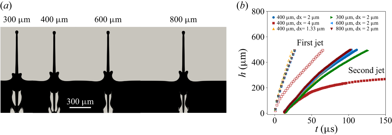
Appendix A. Simulation sensitivity to domain size and resolution
For the simulations we confirmed insensitivity to both lateral domain size and grid resolution by performing simulations at different lateral domain sizes of 300, 400, 600 and 800  $\mathrm {\mu }$m, and at uniform resolutions of
 ${{\rm d} x} = 4$
 $\mathrm {\mu }$m,
 ${{\rm d} x} = 2$
 $\mathrm {\mu }$m and
 ${{\rm d} x} = 1.33$
 $\mathrm {\mu }$m. We found no significant change for a lateral domain size larger than 400
 $\mathrm {\mu }$m or a resolution smaller than
 ${{\rm d} x} = 2$
 $\mathrm {\mu }$m. In figure 8(a) we show snapshots of simulations at
 $t = 25$
 $\mathrm {\mu }$s after initiation. As the jet time series in figure 8(b) confirms, lateral domains widths of 400
 $\mathrm {\mu }$m and a resolution of
 ${{\rm d} x} = 2$
 $\mathrm {\mu }$m are sufficient to achieve insensitivity to these parameter choices. We thus adopted these values for the simulations.
(a) Snapshots of simulations (vertical slices) at  $t = 25$
 $\mathrm {\mu }$s after initiation for different domain widths. (b) Time series of first jet (open symbols) and second jet (closed symbols) positions for these same domain widths as well as two different resolutions
 ${{\rm d} x}$. For domain sizes larger than 300
 $\mathrm {\mu }$m and resolutions smaller than
 ${{\rm d} x} = 4$
 $\mathrm {\mu }$m, the results do not differ significantly.

Appendix B. Rayleigh–Plesset numerical solution
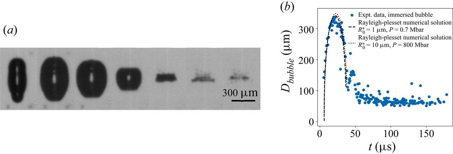
An additional estimate of the initial experimental bubble pressure is obtained by comparing the oscillations of the bubble diameter with the predictions of the Rayleigh–Plesset equation (see figure 9) (Lauterborn & Kurz Reference Lauterborn and Kurz2010). In this case, the bubble was initiated far from the interface to avoid its influence on the dynamics. We solve the Rayleigh–Plesset equation for the radius  $R$ including the effects of viscosity and surface tension
 \begin{equation} \rho R \frac{{\rm d}^2 R}{{\rm d}t^2} + \frac{3}{2} \rho \left( \frac{{\rm d}R}{{\rm d}t} \right)^2 = P \left( \frac{R_0}{R} \right)^{3 \kappa} - P_{\infty} - \frac{4 \mu}{R} \frac{{\rm d}R}{{\rm d}t} - \frac{2 \sigma}{R}, \end{equation}
where  $P$ and
 $R_0$ are the initial pressure and radius of the bubble at rest,
 $\kappa = 4/3$ is the isentropic expansion factor of water,
 $P_{\infty } = 1$ bar is the pressure at infinity,
 $\mu = 8.9\times 10^{-4}$ kg m
 $^{-1}$ s is the dynamic viscosity of water and
 $\sigma = 0.072$ N m
 $^{-1}$ is the surface tension between water and air. This equation is integrated forward in time using a fourth-order Runge–Kutta method. Because the experimental bubble is axisymmetric, we plot a diameter that accommodates for the cigar shape of the bubble so that we can better compare with the Rayleigh–Plesset theory for symmetric spherical bubbles:
 $D_{bubble} = (D_v D_h ^2)^{1/3}$, where
 $D_v$ is the vertical length and
 $D_h$ is the shorter radial width. We found empirically that at their maximum values
 $D_h/D_v \simeq 0.41$, which is close to the value of
 $\beta = 0.48$ used in figure 7(c). We estimated initial bubble diameters of
 $R_0 \simeq 1$
 $\mathrm {\mu }$m in § 3 (see figure 7d). Assuming that this
 $R_0$ corresponds to the smaller horizontal width of the bubble, and using the same ratio of vertical to horizontal length scales found in experiments, the effective initial bubble size used in the numerical solution of the Rayleigh–Plesset equation is then
 $R_0^* = (R_0^2 (D_v R_0 / D_h )) ^{1/3} \simeq 1.3$
 $\mathrm {\mu }$m. We find that an estimate of
 $P = 0.7$ Mbar gives excellent agreement both in terms of spatial and temporal magnitude with the experimental observations, and is close to the estimated value of
 $P \sim 3$ Mbar found using (3.1).
(a) Sequence of side-view images illustrating the laser pulse interaction with the liquid. The laser pulse energy is  $E = 0.915$ mJ. Here, the laser pulse was focused with a
 $\times 50$ magnification microscope objective. Dynamics of a bubble, the black region, nucleated at a large depth (
 $H = \infty$) far from any interface. The time between images is 9
 $\mathrm {\mu }$s. The bubble shape is axisymmetric but not spherical, a result of the non-spherical focused laser spot. (b) Plot of immersed bubble diameter
 $D_{bubble}$ vs time
 $t$ from experiments. The laser energy used to initiate this bubble is
 $E = 18.3$
 $\mathrm {\mu }$J. We also plot the numerical solution when
 $R_0 = 10$
 $\mathrm {\mu }$m (
 $R_0^* \simeq 13.4$
 $\mathrm {\mu }$m), which fits with the experiments when
 $P = 800$ bar. This result is consistent with
 $PR_0^3 = {\rm const.}$, as argued for figure 7(d).

Appendix C. Dependence of droplet and bubble diameter
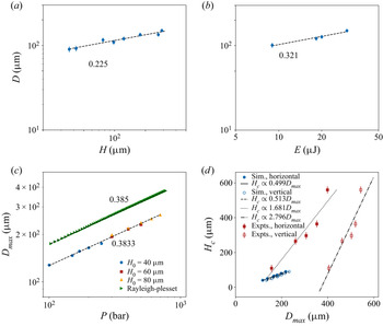
Here, we present the droplet and bubble diameter dependence on parameters such as the initial depth  $H$, the initial energy
 $E$ or pressure
 $P$. The main significance of this presentation is that the droplet diameter
 $D$ is only weakly dependent on these control parameters, and that the maximum bubble diameter
 $D_{max}$ is the dominant length scale. In figure 10(a) we show the dependence of the experimental droplet diameter
 $D$ on the depth
 $H$, which follows a weak power law,
 $D \propto H^{0.225}$. In figure 10(b) we show the dependence of
 $D$ on the initial energy
 $E$, which is also a weak power law,
 $D \propto E^{0.321}$. We are not aware of any theory that accounts for these power laws. The dependence of the maximum bubble diameter in simulations,
 $D_{max}$ on pressure
 $P$ is shown in figure 10(c). This also follows a weak power law,
 $D_{max} \propto P^{0.383}$ that is consistent with prediction from the Rayleigh–Plesset equation (see Appendix B). Finally, figure 10(d) shows the dependence of the critical depth
 $H_c$ on the maximum bubble diameter
 $D_{max}$ for both simulations and experiments. The dependence is essentially linear, and is in keeping with our finding that
 $D_{max}$ is the dominant length scale and thus can be used to collapse the plots of velocity vs depth (see figure 7c). While in simulations the horizontal and vertical maximum bubble diameters are essentially the same, they differ significantly in experiments. That the experiments and simulations should belong to different curves is not surprising, given the differences between them such as initial bubble size and asymmetry. The significance of figure 10(d) is that
 $D_{max}$ sets the critical depth
 $H_c$, just as it also sets the droplet diameter (see figure 6a).
(a) Plot of second jet droplet diameter  $D$ vs initial depth
 $H$ for experiments at fixed energy
 $E = 18.3$
 $\mathrm {\mu }$J. (b) Plot of second jet droplet diameter
 $D$ vs energy
 $E$ for fixed initial depth
 $H = 125$
 $\mathrm {\mu }$m. Unlike the second jet velocity, the droplet diameter
 $D$ is relatively insensitive to variations in either
 $H$ or
 $E$. (c) Plot of horizontal maximum bubble diameter
 $D_{max}^h$ vs initial pressure
 $P$ for simulations at different depths and the numerical solution of the Rayleigh–Plesset equation. Although the results from simulations are below the prediction of the Rayleigh–Plesset equation, which unlike the simulations assumes the fluid surrounding the bubble extends to infinity in all directions,
 $D_{max}^h \propto P^{0.38}$ for both. (d) The empirically determined critical depths
 $H_c$ vs empirically determined vertical
 $D_{max}^v$ and horizontal
 $D_{max}^h$ maximum submerged bubble diameters. While both depend on
 $E$ or
 $P$,
 $H_c$ and
 $D_{max}$ are strongly correlated. While for simulations the
 $D_{max}^h \simeq D_{max}^v$, the asymmetry of the initial bubble in experiments results in
 $D_{max}^v$ being nearly twice as large as
 $D_{max}^h$.

Appendix D. Dependence on initial bubble shape
In nearly all of the simulations presented the initial bubble was spherical with radius  $R_0 = 10$
 $\mathrm {\mu }$m. In this appendix we present the results of simulations with the same initial volume, and thus the same initial energy
 $P R_0^3$, but with an initially elliptical shape. The ratio of the vertical to horizontal length was 2. Keeping the initial bubble pressure fixed at
 $P = 200$ bar, we varied the position of the centre of the bubble
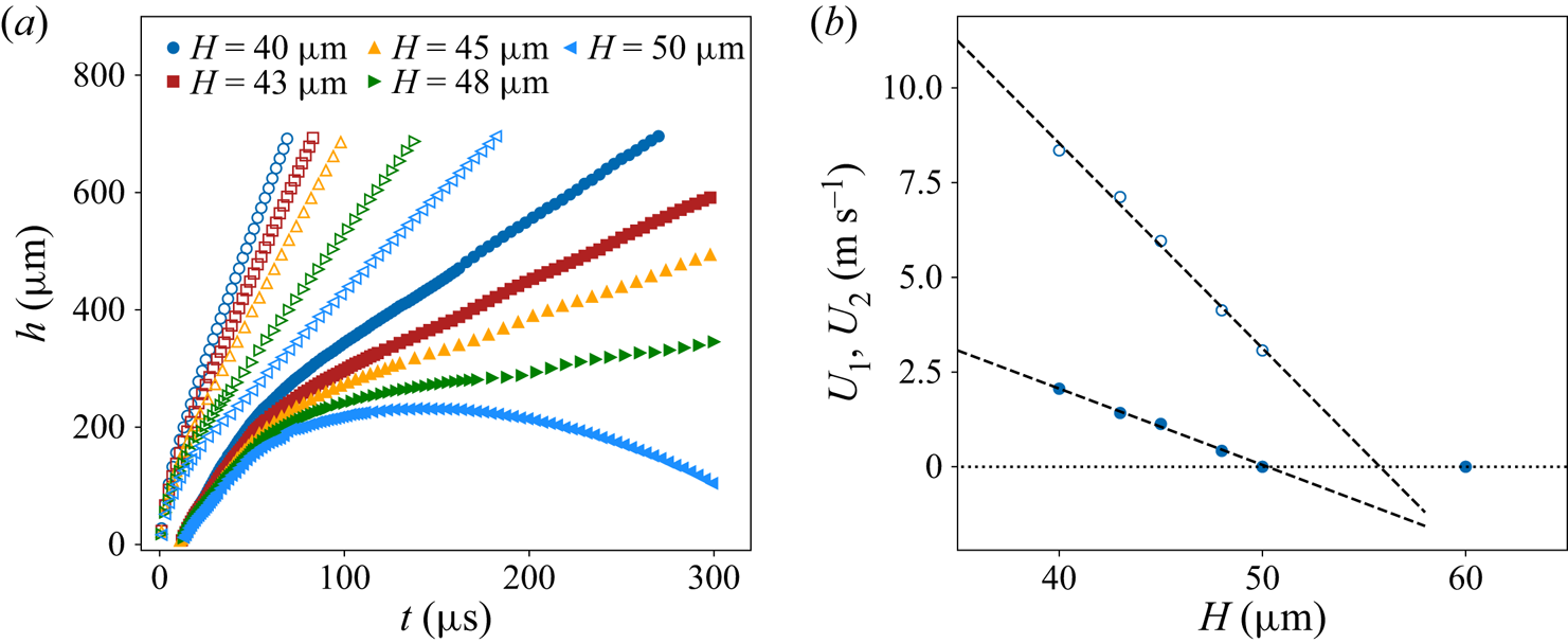
 $H$. Figure 11(a) reveals jet time series of the same character as figure 2(c), with
 $U_1$ and
 $U_2$ steadily decreasing with increasing
 $H$ as shown in figure 11(b). Likewise the plot of
 $U_1$ and
 $U_2$ vs
 $H$ in figure 11(b) is similar to figures 5(b) and 7(b), with an approximately linear dependence of the asymptotic velocities on
 $H$ near a critical
 $H_c$, although the critical
 $H_c$ for the first and second jet is slightly different. The normalized velocities are included in figure 7(c) with
 $\beta \simeq 0.48$ as with the other simulations. The simulations collapse on themselves regardless of the initial bubble shape. Consistent with this, the maximum vertical bubble diameter
 $D_{max}^v$ differs little from the horizontal diameter
 $D_{max}^h$, despite the different initial shape.
(a) Jet height  $h$ vs time
 $t$ for different
 $H$ and fixed initial pressure
 $P = 200$ bar for an initially elliptic bubble. The first jet is indicated by open symbols. The same qualitative trends and phenomenology is observed as for simulations with an initially spherical bubble (see figure 2c). (b) Plot of the first
 $U_1$ and second
 $U_2$ jet velocity vs
 $H$ for fixed
 $P = 200$ bar from simulations for an initially elliptic bubble. Both vary approximately linearly near a threshold value of
 $H_c \simeq 50$
 $\mathrm {\mu }$m.