





1 Introduction
Stratified multilayer plane channel flows involving more than one interface emerge in a large number of industrial applications and exhibit unique nonlinear behaviour. Importantly, such geometrically complex flows raise physical and mathematical issues that are not encountered in two-fluid single-interface channel flows, which have been studied extensively. Flows with multiple interfaces depend on many physical parameters, but more crucially their interfacial dynamics support nonlinear mechanisms between the interacting interfaces and which, in turn, induce inertialess instabilities, that are not found in two-fluid single-interface flows, (Chen Reference Chen1995; Pozrikidis Reference Pozrikidis2004).
The stability of three-layer Couette flow was first studied by Li (Reference Li1969), who predicted that long-wave instability is possible even in the absence of inertia. Motivated by Li’s study, Kliakhandler & Sivashinsky (Reference Kliakhandler and Sivashinsky1995) considered a three-layer plane Poiseuille flow in the absence of inertia and identified two kinds of long-wave instabilities in the weakly nonlinear regime. One (first kind) due to the coupled linear advective terms supporting complex eigenvalues, and one (second kind) due to the interaction between the linear advection and interfacial tension terms. The second kind of inertialess instability can be understood mathematically as a generalised Majda–Pego (Majda & Pego Reference Majda and Pego1985) instability for fourth-order dissipation due to interfacial tension. Note that in the case of open multilayer flows when one interface and a free surface are present, it has been observed that the first kind of inertialess instability is absent (Weinstein & Kurz Reference Weinstein and Kurz1991; Kliakhandler & Sivashinsky Reference Kliakhandler and Sivashinsky1997).
Typically, the inertialess instabilities described above are assumed to emerge exclusively due to linear mechanisms. However, it has been shown recently by Papaefthymiou, Papageorgiou & Pavliotis (Reference Papaefthymiou, Papageorgiou and Pavliotis2013) that inertialess instabilities in multilayer flows can also emerge due to nonlinear dynamics of the interfaces. Linear theories (used extensively in the case of single-interface flows) are not sufficient for stability when multiple interfaces are present. In this study we draw attention to a nonlinear physical phenomenon encountered in multilayer flows, namely the nonlinear transition of an initially stable flow to an unstable one driven by inertialess instabilities that develop in time. We term this nonlinear phenomenon as transitional instabilities (these are distinct from linear transient growth phenomena, see Trefethen et al. (Reference Trefethen, Thefethen, Reddy and Driscoll1993) for example).
Such transitional instabilities have been identified in the context of
 $2\times 2$
systems of conservation laws of mixed hyperbolic–elliptic type. By considering the initial value problem of mixed hyperbolic–elliptic systems and starting with smooth initial conditions that ensure the systems are everywhere hyperbolic (i.e. the Jacobian of the flux function possesses real eigenvalues), these systems may remain hyperbolic throughout their evolution or transition to ellipticity (i.e. develop complex conjugate eigenvalues). This phenomenon has been encountered in different fluid applications – (Bürger et al.
Reference Bürger, Karlsen, Tory and Wendland2002; Jackson & Blunt Reference Jackson and Blunt2002; Talon et al.
Reference Talon, Martin, Rakotomalala, Salin and Yortsos2004; Chumakova et al.
Reference Chumakova, Menzaque, Milewski, Rosales, Tabak and Turner2009; Boonkasame & Milewski Reference Boonkasame and Milewski2012) – and has raised concern regarding the physical relevance of the mathematical models. Due to the absence of dissipative mechanisms in systems of conservation laws, the existence of ellipticity introduces a catastrophic instability in the sense of Hadamard – (Joseph & Saut Reference Joseph and Saut1990). In the problem of viscous multilayer channel flows presented here, the phenomenon of hyperbolic–elliptic transition corresponds to the case when the first kind of inertialess instability mentioned previously emerges. Importantly, the models derived and studied here are regularised systems of conservation laws that are well-posed and perfect physical candidates for the study of this transitional nonlinear behaviour.
In this paper we focus on the case of pressure- and gravity-driven three-layer flows inside an inclined channel. We derive weakly nonlinear models (valid for long waves of small amplitude) and analyse them in order to understand the nonlinear phenomenon of transitional instability described above. The derived mathematical models are
 $2\times 2$
semi-linear parabolic systems and one can distinguish two possible physical dissipative mechanisms; fourth-order dissipation due to strong interfacial tension, and/or second-order dissipation due to stable density stratification. In this paper we focus on the latter case by considering small channel inclinations and promoting second-order parabolic systems where rigorous nonlinear theory can be applied. In channel flows (unlike open flows – see references above), weakly nonlinear systems can be derived asymptotically correctly due to Galilean invariance, i.e. equal eigenvalues. Note that Galilean invariance is related to the existence of instability of the first kind (complex eigenvalues), since the system must cross equal eigenvalues before they become complex. Finally, we stress that the deep understanding and prediction of the behaviour of such complex flows demands the departure from well-established linear theories (albeit sufficient in two-layer flows) and the development of nonlinear methods.
2 Formulation and mathematical models
Consider a plane channel flow comprised of three immiscible incompressible viscous Newtonian fluids, driven by gravity and an imposed pressure gradient along the channel – see figure 1. The fluid dynamics are governed by the Navier–Stokes equations in each phase, and sufficiently strong interfacial tension is present at the two fluid–fluid interfaces – see Chang, Demekhin & Kopelevich (Reference Chang, Demekhin and Kopelevich1993). At low and moderate Reynolds numbers
 $Re=\unicode[STIX]{x1D70C}_{1}U\,d/\unicode[STIX]{x1D707}_{1}$
, where
 $U$
is a typical flow velocity,
 $d$
is the channel height and
 $\unicode[STIX]{x1D70C}_{1}$
,
 $\unicode[STIX]{x1D707}_{1}$
are the density and viscosity of the upper fluid, such multilayer flows remain immiscible and can become unstable, producing two-dimensional interfacial wave dynamics. As discussed in the Introduction, it is sufficient to consider inertialess flows (i.e.
 $Re\approx 0$
), and also long waves due to the presence of interfacial tension and/or stable density stratification that act to damp short waves. This leads to the nonlinear partial differential equations (PDEs) (2.3) that are amenable to analysis and computations.
Schematic of a three-layer flow down an inclined plane channel.
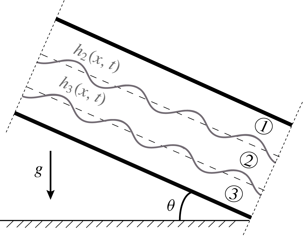
The boundary conditions are those of no-slip at the walls along with continuity of velocities, balance of normal and tangential stresses, and kinematic conditions at the interfaces. In addition, periodic boundary conditions are imposed in the direction along the channel. Introducing a small parameter
 $\unicode[STIX]{x1D6FF}\ll 1$
measuring the ratio of the channel height
 $d$
to a typical interfacial wavelength, and carrying out an asymptotic expansion of the governing equations and boundary conditions to second order, leads to a system that involves
 $O(1)$
and
 $O(\unicode[STIX]{x1D6FF})$
terms (for details of the analysis see Papaefthymiou et al. (Reference Papaefthymiou, Papageorgiou and Pavliotis2013)). The reduced system in terms of the dimensionless independent variables
 $\unicode[STIX]{x1D709}$
(spatial) and
 $\unicode[STIX]{x1D70F}$
(temporal) reads
 $$\begin{eqnarray}\boldsymbol{h}_{\unicode[STIX]{x1D70F}}+\boldsymbol{F}(\boldsymbol{h},\boldsymbol{T})_{\unicode[STIX]{x1D709}}+\unicode[STIX]{x1D6FF}\left[\left(Re\,\unicode[STIX]{x1D64E}(\boldsymbol{h},\boldsymbol{T})+\cot \unicode[STIX]{x1D703}\unicode[STIX]{x1D642}(\boldsymbol{h},\boldsymbol{T})\right)\boldsymbol{h}_{\unicode[STIX]{x1D709}}+\frac{1}{\overline{C}_{a}}\unicode[STIX]{x1D63F}(\boldsymbol{h},\boldsymbol{T})\boldsymbol{h}_{\unicode[STIX]{x1D709}\unicode[STIX]{x1D709}\unicode[STIX]{x1D709}}\right]_{\unicode[STIX]{x1D709}}=0,\end{eqnarray}$$
and we emphasise that retention of
 $\unicode[STIX]{x1D6FF}$
terms is crucial in providing a dissipative regularisation to prevent overturning or catastrophic short wave instabilities. In (2.1)
 $\boldsymbol{h}(\unicode[STIX]{x1D709},\unicode[STIX]{x1D70F})=(h_{2},h_{3})^{\text{T}}$
is the vector of the dimensionless interfacial positions (the superscript
 $\text{T}$
denotes transpose) and is always positive and
 $2L$
-periodic, i.e.
 $\boldsymbol{h}(\unicode[STIX]{x1D709}+2L,\unicode[STIX]{x1D70F})=\boldsymbol{h}(\unicode[STIX]{x1D709},\unicode[STIX]{x1D70F})$
. The
 $2\times 1$
nonlinear flux vector
 $\boldsymbol{F}$
and the
 $2\times 2$
matrices
 $\unicode[STIX]{x1D64E}$
,
 $\unicode[STIX]{x1D642}$
and
 $\unicode[STIX]{x1D63F}$
have terms that are rational polynomial functions of the interfacial deformations
 $h_{2,3}$
, as well as the vector of the dimensionless physical parameters of the problem
 $\boldsymbol{T}$
. The latter is defined as
 $$\begin{eqnarray}\boldsymbol{T}\equiv (H_{2},H_{3},m_{2},m_{3},r_{2},r_{3})^{\text{T}},\end{eqnarray}$$
where
 $m_{2,3}$
and
 $r_{2,3}$
are the viscosity and density ratios in regions
 $2$
and
 $3$
non-dimensionalised with respect to the properties of the top layer region
 $1$
, while
 $H_{2,3}$
are the undisturbed interfacial positions, i.e. the spatial means of
 $h_{2}(\unicode[STIX]{x1D709},\unicode[STIX]{x1D70F})$
and
 $h_{3}(\unicode[STIX]{x1D709},\unicode[STIX]{x1D70F})$
. The dimensionless channel height is
 $1$
. The scaled capillary number
 $\overline{C}_{a}=O(1)$
derives from strong interfacial tension so that
 $Ca=\unicode[STIX]{x1D6FF}^{2}\overline{C}_{a}$
, where
 $Ca=2U\unicode[STIX]{x1D707}_{1}/\unicode[STIX]{x1D70E}$
is the capillary number, and
 $\unicode[STIX]{x1D70E}$
is the interfacial tension taken to be the same at the two interfaces;
 $\unicode[STIX]{x1D703}$
measures the angle of the channel with respect to the horizontal as shown in figure 1. The system (2.1) is a generalisation of the scalar Benney equation (Benney Reference Benney1966) that was derived for two-fluid flows with a single interface, and incorporates inertia, buoyancy and interfacial tension effects through the matrices
 $\unicode[STIX]{x1D64E}$
,
 $\unicode[STIX]{x1D642}$
and
 $\unicode[STIX]{x1D63F}$
, respectively.
Our goal is to understand the fundamental nonlinear inertialess instabilities of (2.1). Inspection shows a competition between second- and fourth-order spatial derivatives. In what follows we derive and study equations that retain second-order dissipative terms alone – physically this can be achieved if interfacial tension is negligible and the combination of inertial and gravitational buoyancy terms provide dissipation. When
 $Re$
is negligible, the gravitational buoyancy term is dissipative if the layers are stably stratified. Mathematically, second-order dissipation in systems is preferable due to the existence of rigorous analytical results that do not extend to fourth-order dissipation. We will construct nonlinear stability criteria based on rigorous mathematics, and subsequently use these as conjectures that can be checked numerically, for higher-order equations when interfacial tension is present.
We simplify (2.1) by taking
 $\unicode[STIX]{x1D703}=O(\unicode[STIX]{x1D6FF})$
, i.e.
 $\cot \unicode[STIX]{x1D703}\approx \unicode[STIX]{x1D6E9}/\unicode[STIX]{x1D6FF}$
where
 $\unicode[STIX]{x1D6E9}>0$
is an order-one constant, which in turn implies that inertial and interfacial tension terms are higher order. The resulting system becomes
 $$\begin{eqnarray}\boldsymbol{h}_{\unicode[STIX]{x1D70F}}+\boldsymbol{F}(\boldsymbol{h},\boldsymbol{T})_{\unicode[STIX]{x1D709}}+(\unicode[STIX]{x1D6E9}\,\unicode[STIX]{x1D642}(\boldsymbol{h},\boldsymbol{T})\boldsymbol{h}_{\unicode[STIX]{x1D709}})_{\unicode[STIX]{x1D709}}=0,\end{eqnarray}$$
and incorporates first-order nonlinear flux functions and second-order nonlinear dissipation due to stable density stratification (
 $r_{3}>r_{2}>1$
) – i.e. matrix
 $\unicode[STIX]{x1D642}$
is negative definite. Similar long-wave models have been derived by Kliakhandler & Sivashinsky (Reference Kliakhandler and Sivashinsky1997) for open multilayer flows down slightly inclined planes. In the present channel flow case, there exist two kinds of long-wave inertialess instabilities supported by system (2.3): (i) when the Jacobian of the flux function possesses complex eigenvalues, and (ii) when these eigenvalues are real but there exists a Majda–Pego instability (Majda & Pego Reference Majda and Pego1985), i.e. an interaction between the flux function and the dissipative term. Finally, we emphasise that the well-posedness of system (2.3) is an open mathematical problem.
One of the most crucial aspects of the kind of interfacial model equations presented above is that linear stability analysis can be misleading regarding the long-time stability of the flow; multilayer flows can encounter instabilities as they evolve nonlinearly in time. This is in contrast to the single-interface scalar case, where linear theory can sufficiently predict instability that can develop into nonlinear states. Consequently, one can raise the following question: given initial conditions for the system (2.3) that are hyperbolic and do not support Majda–Pego instability, under what criteria will the system remain nonlinearly stable throughout its spatiotemporal evolution?
We will address this question under the additional assumption of weakly nonlinear dynamics along with the scenario where the layers close to the walls of the channel are thin compared to the middle layer. This simplifies system (2.1) (i.e. matrix
 $\unicode[STIX]{x1D642}$
becomes now a multiple of the identity matrix) and enables us to apply a mathematical theory to derive sufficient conditions for nonlinear stability. Such conditions provide insight and directions for future studies regarding the more challenging case of the full nonlinear systems (2.1) and (2.3).
2.1 Weakly nonlinear dynamics
Weakly nonlinear dynamics emerge for sufficiently small interfacial amplitudes. In appendix A, we start with (2.1) and provide detailed physical and asymptotic justifications for stably stratified flows with negligible inertia and interfacial tension, to derive the weakly nonlinear models studied in this paper. This scenario yields the following semi-linear parabolic system
 $$\begin{eqnarray}\boldsymbol{\unicode[STIX]{x1D702}}_{t}+\unicode[STIX]{x1D65B}(\boldsymbol{\unicode[STIX]{x1D702}},\boldsymbol{Z})\boldsymbol{\unicode[STIX]{x1D702}}_{x}-\unicode[STIX]{x1D708}\unicode[STIX]{x1D644}\boldsymbol{\unicode[STIX]{x1D702}}_{xx}=0,\end{eqnarray}$$
where the scaled interfacial amplitudes
 $\boldsymbol{\unicode[STIX]{x1D702}}=(\unicode[STIX]{x1D702}_{1},\unicode[STIX]{x1D702}_{2})^{\text{T}}$
are
 $2\unicode[STIX]{x03C0}$
-periodic and have zero spatial mean,
 $\unicode[STIX]{x1D644}$
is the identity matrix (which is of course symmetric and positive definite) which excludes the possibility of Majda–Pego instability. Furthermore, the matrix
 $\unicode[STIX]{x1D65B}$
and the bifurcation parameter
 $\unicode[STIX]{x1D708}>0$
are defined in appendix A. The only instability present in (2.4) arises when the matrix
 $\unicode[STIX]{x1D65B}$
possesses complex conjugate eigenvalues (ellipticity). This is possible for certain values of the perturbed physical parameters
 $\boldsymbol{Z}$
(see appendix A for a definition of this constant vector) and the dependent variables
 $\boldsymbol{\unicode[STIX]{x1D702}}$
for some values of
 $x$
and
 $t$
. Complex eigenvalues induce instability that depends on the evolving solutions; we emphasise that linear stability analysis about uniform states is unable to predict the long-time behaviour of system (2.4) when the eigenvalues are initially real (hyperbolicity). Next we will present a nonlinear theory to derive a criterion that can answer the question posed previously, but for the weakly nonlinear system (2.4). In the case of instability, numerical solutions will be used to construct the ultimate nonlinear states.
3 Nonlinear stability theory for multilayer flows
At this stage it is important to briefly introduce the concept of invariant regions that has been developed in the context of second-order nonlinear parabolic systems by Chueh, Conley & Smoller (Reference Chueh, Conley and Smoller1977). Their theorems prove the existence of invariant regions in the solution state space of certain nonlinear parabolic systems, implying solutions are confined to these regions for all times. We will use these results to develop a nonlinear stability theory for the present multilayer flow systems; these are distinguished from those studied by Chueh et al. (Reference Chueh, Conley and Smoller1977) in that they can transition from hyperbolicity to ellipticity.
Geometrically, invariant regions are formed due to the convexity of two families of integral curves that span the hyperbolic state space (
 $\unicode[STIX]{x1D702}_{1},\unicode[STIX]{x1D702}_{2}$
) of system (2.4). These parametric curves are tangent to the vector field produced by the right eigenvectors of the matrix
 $\unicode[STIX]{x1D65B}$
, and therefore are solutions of the following ordinary differential equations (ODEs):
 $$\begin{eqnarray}\frac{\text{d}\unicode[STIX]{x1D702}_{2}}{\text{d}\unicode[STIX]{x1D702}_{1}}=\frac{2\unicode[STIX]{x1D627}_{21}}{\unicode[STIX]{x1D627}_{11}-\unicode[STIX]{x1D627}_{22}\pm \sqrt{(\unicode[STIX]{x1D627}_{11}-\unicode[STIX]{x1D627}_{22})^{2}+4\unicode[STIX]{x1D627}_{12}\unicode[STIX]{x1D627}_{21}}},\end{eqnarray}$$
when
 $\unicode[STIX]{x1D627}_{21},\unicode[STIX]{x1D627}_{12}\neq 0$
and where
 $\unicode[STIX]{x1D627}_{ij}$
are the elements of matrix
 $\unicode[STIX]{x1D65B}$
and
 $(-)$
corresponds to the first family of the integral curves, while
 $(+)$
corresponds to the second family. In fluid mechanics language, the families of integral curves introduced above are mathematically equivalent to the geometrical concept of streamlines in a flow, i.e. they are defined as a family of integral curves that are tangent to the velocity vector field of a flow. Furthermore, such curves are known as rarefaction curves or wave curves in the context of hyperbolic conservation laws, (Smoller Reference Smoller1994).
Importantly, we observe that one can identify special bounded invariant regions in the state space, when the matrix
 $\unicode[STIX]{x1D65B}$
possesses real eigenvalues. In particular, given initial conditions contained within these bounded hyperbolic invariant regions, then the evolution of the system remains confined to them, thus preventing crossing into elliptic regions. This in turn implies nonlinear stability of the system, with solutions decaying to trivial steady states
 $(\boldsymbol{\unicode[STIX]{x1D702}}=0)$
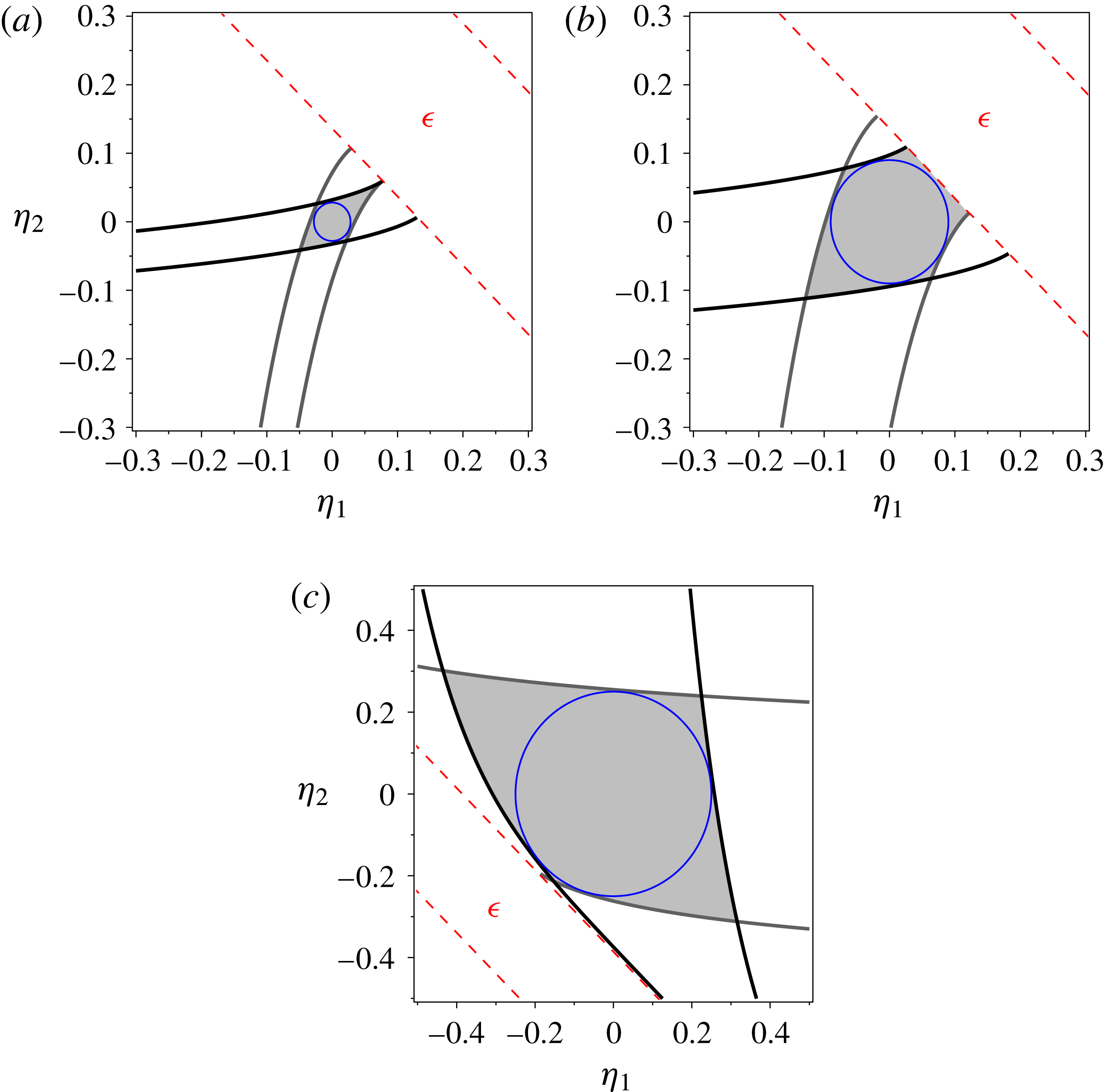
at large times. In the present study we use spatially periodic initial conditions which mainly correspond to closed curves in the state space (typically circles for sinusoidal varicose initial data, for example). Nonlinear stability follows if there exist four rarefaction curves, two from each family, that tangentially bound the initial conditions, and so defining minimal invariant regions – examples are illustrated below.
Bounding integral curves given by ODEs (3.1) in the
 $(\unicode[STIX]{x1D702}_{1},\unicode[STIX]{x1D702}_{2})$
-space of system (2.4), where grey curves correspond to the first family of the integral curves and black ones to the second family. Initial hyperbolic conditions are depicted by circles, the dashed lines are the boundaries of the elliptic region (
 $\unicode[STIX]{x1D716}$
), while shaded regions denote the minimum invariant region for the corresponding initial conditions. (a,b) correspond to matrix
 $\unicode[STIX]{x1D65B}$
given by (3.2), while in the case of (c), matrix
 $\unicode[STIX]{x1D65B}$
is given by (3.3).
To fix and demonstrate ideas, we consider the physical scenario where the density and viscosity of the configuration decrease from the bottom to the top layer of the channel. Furthermore the outer layers are thinner than the middle layer. Specifically, following the analysis presented in appendix A, we consider the perturbed parameter vector
 $\boldsymbol{Z}=(-7/8,9/16,27/16)^{\text{T}}$
, and the matrix
 $\unicode[STIX]{x1D65B}$
in system (2.4) is calculated to be
 $$\begin{eqnarray}\unicode[STIX]{x1D65B}=\left[\begin{array}{@{}cc@{}}\displaystyle -{\textstyle \frac{3}{8}}-2\unicode[STIX]{x1D702}_{1} & \displaystyle -{\textstyle \frac{1}{4}}\\ \displaystyle {\textstyle \frac{1}{8}} & \displaystyle -1+2\unicode[STIX]{x1D702}_{2}\end{array}\right].\end{eqnarray}$$
This physical scenario supports real eigenvalues of
 $\unicode[STIX]{x1D65B}$
when
 $\unicode[STIX]{x1D702}_{1}=\unicode[STIX]{x1D702}_{2}=0$
; as a result, linear stability analysis predicts that disturbances proportional to
 $\text{e}^{\text{i}kx+st}$
decay exponentially in time for all wavenumbers
 $k$
. Now let us apply the nonlinear stability theory described above when
 $\unicode[STIX]{x1D65B}$
is given by (3.2). The bounding integral curves produced by ODEs (3.1) in the hyperbolic
 $(\unicode[STIX]{x1D702}_{1},\unicode[STIX]{x1D702}_{2})$
-space are depicted in figure 2(a,b) for two different periodic initial conditions indicated by circles (even though it may be possible to solve (3.1) in closed form, it is straightforward to solve them numerically). Note that regions denoted by (
 $\unicode[STIX]{x1D716}$
) in the figures are elliptic (complex eigenvalues) and the dashed lines denote the boundaries between hyperbolic and elliptic regions. In the case of sufficiently small initial conditions, i.e.
 $\boldsymbol{\unicode[STIX]{x1D702}}=(0.028\cos (x),0.028\sin (x))^{\text{T}}$
, figure 2(a) depicts the integral curves that form a bounded hyperbolic invariant region (grey shaded region). Hence, solutions of system (2.4) will not cross the hyperbolic–elliptic boundary. However, in the case of larger hyperbolic initial conditions
 $\boldsymbol{\unicode[STIX]{x1D702}}=(0.09\cos (x),0.09\sin (x))^{\text{T}}$
, the minimal invariant region shaded grey in figure 2(b) is unbounded, and hence the solutions can cross into the elliptic region as they evolve in time depending on the amount of dissipation that is present – this is discussed in detail later.
Before we proceed to our next scenario, we would like to illustrate the effect of different initial conditions having the same initial energy, when
 $\unicode[STIX]{x1D65B}$
is given by (3.2). The energy is chosen to be
 $0.1629$
and the hyperbolic initial conditions are: case (i)
 $\boldsymbol{\unicode[STIX]{x1D702}}=(0.065\cos (x),0.065\sin (x))^{\text{T}}$
, and case (ii)
 $\boldsymbol{\unicode[STIX]{x1D702}}=(0.065\cos (x),0.065\cos (x))^{\text{T}}$
. The integral curves, constructed as above, are given in figure 3(a,b) for cases (i) and (ii), respectively. For case (i) there is no bounded invariant region and the system can transition into the elliptic region for a sufficiently small value of dissipation
 $\unicode[STIX]{x1D708}$
. For case (ii), however, figure 3(b) shows that the initial condition lies inside a bounded invariant region, and this guarantees that the system will not cross into the elliptic region, and hence will be stable for arbitrarily small values of
 $\unicode[STIX]{x1D708}$
. Therefore, our nonlinear analysis predicts that nonlinear stability depends crucially on the geometrical structure of the initial conditions in the
 $(\unicode[STIX]{x1D702}_{1},\unicode[STIX]{x1D702}_{2})$
-space. Potentially, nonlinear stability can be achieved for classes of initial conditions of arbitrary energy. However, if we restrict the initial conditions to be of the sinusoidal varicose form used to produce the results of figure 2 (i.e. circles), then we can compute the minimum seed that may trigger transition to ellipticity, depending on the amount of dissipation. This minimal energy was found to be above
 $0.072$
, correct to three decimals, as can be predicted by figure 2(a).
For our next scenario we introduce a slightly different matrix
 $$\begin{eqnarray}\unicode[STIX]{x1D65B}=\left[\begin{array}{@{}cc@{}}\displaystyle -{\textstyle \frac{3}{8}}-2\unicode[STIX]{x1D702}_{1} & \displaystyle -{\textstyle \frac{1}{4}}\\ \displaystyle {\textstyle \frac{1}{8}} & \displaystyle {\textstyle \frac{3}{4}}+2\unicode[STIX]{x1D702}_{2}\end{array}\right],\end{eqnarray}$$
which corresponds to the perturbed parameter vector
 $\boldsymbol{Z}=(0,9/16,27/16)^{\text{T}}$
; physically, we have slightly increased the width of the bottom layer (this is the most viscous layer) compared to the previous physical configuration. Matrix
 $\unicode[STIX]{x1D65B}$
once again possesses real eigenvalues about
 $\boldsymbol{\unicode[STIX]{x1D702}}=0$
. However, as shown in figure 2(c), the second family of integral curves do not cross the hyperbolic–elliptic boundary but only reach it asymptotically. Importantly, such behaviour guarantees the formation of bounded hyperbolic invariant regions for any strictly hyperbolic initial conditions (here strictly means that points on the hyperbolic–elliptic boundary are excluded from the initial conditions). In figure 2(c) we present the minimal invariant region when the initial conditions are given by
 $\boldsymbol{\unicode[STIX]{x1D702}}=(0.25\cos (x),0.25\sin (x))^{\text{T}}$
. Therefore, we can conclude that in the case of matrix (3.3), system (2.4) is nonlinearly stable for arbitrarily large strictly hyperbolic initial conditions (it is understood that the weakly nonlinear assumption remains valid), i.e. the solutions will decay to zero at large times without encountering ellipticity. Finally, we would like to emphasise that the two distinct scenarios presented in this section constitute the canonical behaviour of the system. The present theory shows how to predict nonlinear stability by studying the integral curves of system (2.4).
Equal energy initial conditions illustrating the different behaviour that exists, when
 $\unicode[STIX]{x1D65B}$
is given by (3.2). (a) Initial conditions
 $\boldsymbol{\unicode[STIX]{x1D702}}=(0.065\cos (x),0.065\sin (x))^{\text{T}}$
; (b) initial conditions
 $\boldsymbol{\unicode[STIX]{x1D702}}=(0.065\cos (x),0.065\cos (x))^{\text{T}}$
.

Numerical experiments for system (2.4) when matrix
 $\unicode[STIX]{x1D65B}$
is given by (3.2) and initial conditions are hyperbolic and are given by the vector
 $\boldsymbol{\unicode[STIX]{x1D702}}=(0.09\cos (x),0.09\sin (x))^{\text{T}}$
. (a) Depicts the evolution of the energy of the system, which is defined as
 $E(t)=\sqrt{\int _{-\unicode[STIX]{x03C0}}^{\unicode[STIX]{x03C0}}(\unicode[STIX]{x1D702}_{1}^{2}+\unicode[STIX]{x1D702}_{2}^{2})\,\text{d}x}$
for various values of the bifurcation parameter
 $\unicode[STIX]{x1D708}$
. (b) Shows the spatiotemporal evolution of the system for
 $\unicode[STIX]{x1D708}=0.01$
in the
 $(\unicode[STIX]{x1D702}_{1},\unicode[STIX]{x1D702}_{2})$
-space up to a time where transition occurs; bold circle marks initial conditions and
 $\unicode[STIX]{x1D716}$
indicates the elliptic region.

3.1 Numerical experiments
In this section we investigate numerically the evolution of the canonical cases presented above. We start with transitional cases (unbounded invariant regions) as exemplified by matrix (3.2) and fixed hyperbolic initial conditions. As expected, if the dissipation
 $\unicode[STIX]{x1D708}$
is sufficiently large, the solutions remain hyperbolic and decay exponentially to trivial states at large times. On the other hand, decreasing
 $\unicode[STIX]{x1D708}$
to moderate values allows the system to transition into the elliptic region, causing growth of the energy initially, before the solutions eventually decay to trivial states once again. This is due to the dissipation pulling the system back to the hyperbolic region. A further decrease of
 $\unicode[STIX]{x1D708}$
enables ellipticity to persist for all time and the system evolves to non-trivial steady-state travelling waves. These three dynamical behaviours are illustrated in the numerical solutions shown in figure 4(a), for
 $\unicode[STIX]{x1D708}=1$
(dashed curve),
 $\unicode[STIX]{x1D708}=0.1$
(dash-dotted curve) and
 $\unicode[STIX]{x1D708}=0.01$
(solid curve), respectively. In all cases the initial conditions are
 $\boldsymbol{\unicode[STIX]{x1D702}}=(0.09\cos (x),0.09\sin (x))^{\text{T}}$
and with energy at 0.2256, corresponding to figure 2(b). These initial conditions are illustrative. Extensive numerical experiments suggest that the system always attains the zero state at large times when
 $\unicode[STIX]{x1D708}=0.1$
or
 $\unicode[STIX]{x1D708}=1$
for various amplitude sinusoidal initial conditions with fixed energy at 0.2256. However, note that this behaviour is attributed to the role of dissipation and it is beyond the validity of our criterion, since for the initial conditions considered, one cannot find bounded invariant regions. The initial stages of transition for
 $\unicode[STIX]{x1D708}=0.01$
in the
 $(\unicode[STIX]{x1D702}_{1},\unicode[STIX]{x1D702}_{2})$
state space is included in figure 4(b). The full evolution in the state space (until travelling waves emerge) is included as supplementary movie 1 available at https://doi.org/10.1017/jfm.2017.605. The corresponding spatiotemporal evolution of the solutions can be found in supplementary movie 2. These numerical results are in full accord with the nonlinear theory described previously and verify the limitations of the linear theory to predict the long-time behaviour of the physical problem.
The no-transition predictions yielding nonlinear stability for the canonical case of matrix (3.3), were verified numerically for the set-up of figure 2. The evolution in the state space for
 $\unicode[STIX]{x1D708}=0.1$
is included as supplementary movie 3. We can conclude, therefore, that the interfacial dynamics are confined to the hyperbolic region for any value of
 $\unicode[STIX]{x1D708}$
(i.e. arbitrarily small) and cannot encounter inertialess instability attaining trivial states at large times.
4 Conclusions
In this paper, we investigated the problem of a three-layer flow inside a slightly inclined channel. The flow is driven by a pressure gradient and gravity, and the fluid layers have different viscosities and densities, the latter having values that provide stably stratified flows. We derived asymptotically correct evolution PDE models capable of describing the nonlinear inertialess evolution of the two interfaces in the long-wave regime. The additional weakly nonlinear limit was analysed to derive systems that incorporate nonlinear flux functions and second-order dissipation. Numerical experiments and nonlinear analysis of these models suggest that multilayer flows can exhibit transitional inertialess instabilities during their evolution. In the nonlinear regime the instabilities saturate to form steady-state interfacial travelling waves. Mathematically, this kind of inertialess instability can be identified through the temporal transition of the flux function from hyperbolicity to ellipticity. We also presented a nonlinear theory which shows that nonlinear stability depends on the existence of bounded invariant regions in the hyperbolic state space of the interfacial. These invariant regions play a crucial role in the nonlinear dynamics in the sense that they prevent transition from occurring.
For the multilayer models studied here, one can distinguish two canonical nonlinear stability cases. The first, when stability depends on the amplitude and/or the geometrical structure of the strictly hyperbolic initial conditions and/or the amount of the dissipation – note that the threshold initial disturbances above which instability can emerge can be predicted by the theory. And, the second, when the flow is nonlinearly stable for all times and for arbitrarily large strictly hyperbolic initial conditions (it is understood that the weakly nonlinear assumption remains valid). Interestingly, the theory predicts that the latter nonlinear stability does not depend on the amount of dissipation present in the flow. Finally, a natural but highly challenging extension of the present work is the study of the phenomenon of nonlinear transition in the case of the fully nonlinear long-wave systems, e.g. (2.1) and (2.3), which account for large interfacial dynamics scaled on the channel height. This is an open problem requiring the development of new techniques that are being considered by the authors.
Acknowledgements
The work of E.S.P. was supported by a EPSRC Doctoral Prize Fellowship. The authors were also supported by EPSRC grants EP/L020564/1 and EP/K041134/1.
Supplementary movies
Supplementary movies are available at https://doi.org/10.1017/jfm.2017.605.
Appendix A. The physical derivation of the weakly nonlinear model (2.4)
We carry out a weakly nonlinear analysis of system (2.1) about the flat interface uniform flow, i.e. we write
 $h_{2,3}(\unicode[STIX]{x1D709},\unicode[STIX]{x1D70F})=H_{2,3}+\unicode[STIX]{x1D6FF}^{3/2}\unicode[STIX]{x1D702}_{1,2}(\unicode[STIX]{x1D709},\unicode[STIX]{x1D70F})$
where
 $\unicode[STIX]{x1D6FF}\ll 1$
. Furthermore, we impose a symmetric configuration with the layers close to the walls being thin and of order
 $\unicode[STIX]{x1D6FF}^{1/4}$
compared to the middle layer; the uniform state is described by the physical parameter vector
 $\boldsymbol{T}=\overline{\boldsymbol{T}}=(1-(\unicode[STIX]{x1D6FF}^{1/4})/3,(\unicode[STIX]{x1D6FF}^{1/4})/3,1,1,1,1)$
– see (2.2) for the definition of
 $\boldsymbol{T}$
– i.e. the three fluids have the same viscosity and density in the base configuration. We proceed by perturbing this base configuration to a nearby steady state that retains stable density stratification but loses the other symmetries due to layer thicknesses and viscosities. More specifically we let
 $\boldsymbol{T}=\overline{\boldsymbol{T}}+\unicode[STIX]{x1D6FF}\tilde{\boldsymbol{T}}_{1}+\unicode[STIX]{x1D6FF}^{5/4}\tilde{\boldsymbol{T}}_{2}+\unicode[STIX]{x1D6FF}^{3/2}\tilde{\boldsymbol{T}}_{3}+\unicode[STIX]{x1D6FF}^{2}\tilde{\boldsymbol{T}}_{4}$
, where
 $\tilde{\boldsymbol{T}}_{1}=(\tilde{H}_{2},-\tilde{H}_{2},\tilde{m}_{2},\tilde{m}_{3},0,0)$
,
 $\tilde{\boldsymbol{T}}_{2}=(0,(\tilde{m}_{3})/3,0,0,0,0)$
,
 $\tilde{\boldsymbol{T}}_{3}=(0,-\tilde{H}_{3},0,0,0,0)$
and
 $\tilde{\boldsymbol{T}}_{4}=(0,0,0,0,2,4)$
. Now, by introducing small angles
 $\unicode[STIX]{x1D703}$
of order
 $\unicode[STIX]{x1D6FF}^{9/4}$
(i.e.
 $\cot \unicode[STIX]{x1D703}\approx \unicode[STIX]{x1D6E9}/\unicode[STIX]{x1D6FF}^{9/4}$
with
 $\unicode[STIX]{x1D6E9}=O(1)$
), we promote second-order dissipation to arrive at the following asymptotically correct equation:
 $$\begin{eqnarray}\boldsymbol{\unicode[STIX]{x1D702}}_{\unicode[STIX]{x1D70F}}+[(\unicode[STIX]{x1D706}_{1}\unicode[STIX]{x1D6FF}^{1/4}+\unicode[STIX]{x1D706}_{2}\unicode[STIX]{x1D6FF}^{1/2}+\unicode[STIX]{x1D706}_{3}\unicode[STIX]{x1D6FF}+\unicode[STIX]{x1D706}_{4}\unicode[STIX]{x1D6FF}^{5/4})\unicode[STIX]{x1D644}+\unicode[STIX]{x1D6FF}^{3/2}\unicode[STIX]{x1D63C}]\boldsymbol{\unicode[STIX]{x1D702}}_{\unicode[STIX]{x1D709}}+3\unicode[STIX]{x1D6FF}^{3/2}\unicode[STIX]{x1D63D}\boldsymbol{\unicode[STIX]{x1D702}}_{\unicode[STIX]{x1D709}}-\frac{4\unicode[STIX]{x1D6E9}}{81}\unicode[STIX]{x1D6FF}^{3/2}\unicode[STIX]{x1D644}\boldsymbol{\unicode[STIX]{x1D702}}_{\unicode[STIX]{x1D709}\unicode[STIX]{x1D709}}+\text{h.o.t.}=0,\end{eqnarray}$$
where
 $\boldsymbol{\unicode[STIX]{x1D702}}=(\unicode[STIX]{x1D702}_{1},\unicode[STIX]{x1D702}_{2})^{\text{T}}$
,
 $\unicode[STIX]{x1D644}$
is the identity matrix,
 $\unicode[STIX]{x1D706}_{1,2,3,4}$
are variables of the physical parameter vector and the matrices
 $\unicode[STIX]{x1D63C}$
and
 $\unicode[STIX]{x1D63D}$
are given by
 $$\begin{eqnarray}\unicode[STIX]{x1D63C}=\frac{2}{3}\left[\begin{array}{@{}cc@{}}\displaystyle (2\tilde{m}_{3}-9\tilde{m}_{2}) & \displaystyle (-\tilde{m}_{3}+\tilde{m}_{2})\\ \displaystyle \tilde{m}_{2} & \displaystyle (5\tilde{m}_{3}-9\tilde{m}_{2}+9\tilde{H}_{3})\end{array}\right],\quad \unicode[STIX]{x1D63D}=\left[\begin{array}{@{}cc@{}}\displaystyle -2\unicode[STIX]{x1D702}_{1} & \displaystyle 0\\ \displaystyle 0 & \displaystyle 2\unicode[STIX]{x1D702}_{2}\end{array}\right].\end{eqnarray}$$
To obtain the final form of the governing equations, we perform a Galilean transformation by introducing new independent variables
 $t^{\prime }=3\unicode[STIX]{x1D6FF}^{3/2}\unicode[STIX]{x1D70F}$
,
 $x^{\prime }=\unicode[STIX]{x1D709}-(\unicode[STIX]{x1D706}_{1}\unicode[STIX]{x1D6FF}^{1/4}+\unicode[STIX]{x1D706}_{2}\unicode[STIX]{x1D6FF}^{1/2}+\unicode[STIX]{x1D706}_{3}\unicode[STIX]{x1D6FF}+\unicode[STIX]{x1D706}_{4}\unicode[STIX]{x1D6FF}^{5/4})\unicode[STIX]{x1D70F}$
. Furthermore, we normalise the equations to
 $2\unicode[STIX]{x03C0}$
-periodic domains by considering new scaled variables
 $t^{\prime \prime }=(\unicode[STIX]{x03C0}/L)^{2}t^{\prime },x^{\prime \prime }=(\unicode[STIX]{x03C0}/L)x^{\prime }$
and defining the bifurcation parameter
 $\unicode[STIX]{x1D708}=4\unicode[STIX]{x03C0}\,\unicode[STIX]{x1D6E9}/243\,L$
which controls the strength of the dissipation in the flow. Finally, dropping double primes and retaining the leading order terms (of size
 $\unicode[STIX]{x1D6FF}^{3/2}$
), yields the following scaled weakly nonlinear system:
 $$\begin{eqnarray}\displaystyle & \displaystyle \boldsymbol{\unicode[STIX]{x1D702}}_{t}+\unicode[STIX]{x1D65B}(\boldsymbol{\unicode[STIX]{x1D702}},\boldsymbol{Z})\boldsymbol{\unicode[STIX]{x1D702}}_{x}-\unicode[STIX]{x1D708}\unicode[STIX]{x1D644}\boldsymbol{\unicode[STIX]{x1D702}}_{xx}=0, & \displaystyle\end{eqnarray}$$
 $$\begin{eqnarray}\displaystyle & \displaystyle \unicode[STIX]{x1D65B}(\boldsymbol{\unicode[STIX]{x1D702}},\boldsymbol{Z})=\left[\begin{array}{@{}cc@{}}\displaystyle \left({\textstyle \frac{4}{9}}\tilde{m}_{3}-2\tilde{m}_{2}-2\unicode[STIX]{x1D702}_{1}\right) & \displaystyle {\textstyle \frac{2}{9}}(-\tilde{m}_{3}+\tilde{m}_{2})\\ \displaystyle {\textstyle \frac{2}{9}}\tilde{m}_{2} & \displaystyle \left({\textstyle \frac{10}{9}}\tilde{m}_{3}-2\tilde{m}_{2}+2\tilde{H}_{3}+2\unicode[STIX]{x1D702}_{2}\right)\end{array}\right], & \displaystyle\end{eqnarray}$$
where we have introduced a new parameter vector defined as
 $\boldsymbol{Z}\equiv (\tilde{H}_{3},\tilde{m}_{2},\tilde{m}_{3})$
.


 Open access

