





1 Introduction
In [Reference LetzterLet99], Letzter introduced what we now call the iquantum groups associated to symmetric pairs. These can be viewed as a generalization of Drinfeld-Jimbo quantum groups – the latter are the iquantum groups arising from diagonal symmetric pairs. Lusztig’s canonical bases for quantum groups, with their favorable positivity properties, provided one source of motivation for the categorification of quantum groups via the Kac-Moody 2-categories of Khovanov, Lauda, and Rouquier [Reference Khovanov and LaudaKL10, Reference RouquierRou08]. A theory of icanonical bases for iquantum groups was developed in [Reference Bao and WangBW18a, Reference Bao and WangBW18b]. In special cases, these again have positive structure constants; see [Reference Li and WangLW18] which treats the quasi-split types AIII. Therefore, it is reasonable to hope that there should be a categorification of iquantum groups.
In rank one, there are three quasi-split iquantum groups of finite type. First, there is the usual
$\mathrm U_q(\mathfrak {sl}_2)$
 , which was categorified by Lauda and Rouquier in [Reference LaudaLau10, Reference RouquierRou08]. The second, arising from the Satake diagram of
$A_2$
 with nontrivial diagram involution, was categorified in [Reference Bao, Shan, Wang and WebsterBSWW18]. In this article, we explain how to categorify the remaining case, the split iquantum group
$\mathrm {U}_q^\imath (\mathfrak {sl}_2)$
 corresponding to the symmetric pair
$(\mathrm {SL}_2,\mathrm {SO}_2)$
 . This is a basic building block for general iquantum groups, and it is expected to play a key role in the categorification of quasi-split iquantum groups of higher rank.
Our categorification of
$\mathrm {U}_q^\imath (\mathfrak {sl}_2)$
 arises from the nil-Brauer category
$\mathbf {NB}_t$
 introduced in [Reference Brundan, Wang and WebsterBWW24]. This is a strict graded
$\Bbbk $
 -linear monoidal category defined over a field
$\Bbbk $
 of characteristic different from 2. It has one self-dual generating object B and four generating morphisms represented diagrammatically by
 (degree 2),
 (degree
$-2$
 ),
 (degree 0), and
 (degree 0), subject to some natural relations recorded in Definition 3.1. The parameter t gives the value of
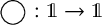 . The defining relations imply that
 ; hence, we must have that
$t=0$
 or
$t=1$
 in order for the category to be nontrivial; see [Reference Brundan, Wang and WebsterBWW24, (2.9)]. We assume that this is the case from now on.
To formulate the main results precisely, rather than working in terms of idempotents, as is often done in the categorification literature, we use the language of modules. By a graded
$\mathbf {NB}_t$
 -module, we mean a graded
$\Bbbk $
 -linear functor from
$\mathbf {NB}_t$
 to graded vector spaces. The endofunctor of
$\mathbf {NB}_t$
 defined by tensoring with its generating object extends to an exact endofunctor, also denoted B, of the category of graded
$\mathbf {NB}_t$
 -modules. Let
$[n] := q^{n-1}+q^{n-3}+\cdots +q^{1-n}$
 be the quantum integer, and
$V^{\oplus [n]}$
 denote the corresponding direct sum of degree-shifted copies of a graded module V.
Theorem A. There are unique (up to isomorphism) indecomposable projective graded
$\mathbf {NB}_t$
 -modules
$P(n)\:(n \geq 0)$
 such that
$P(0)$
 is the projective graded module associated to the idempotent that is the identity endomorphism of the unit object, and for
$n \geq 0$
 we have that

interpreting
$P(-1)$
 as 0. These modules give a full set of indecomposable projective graded
$\mathbf {NB}_t$
 -modules (up to isomorphism and grading shift).
The proof of Theorem A is similar in spirit to Lauda’s proof of the analogous result for the 2-category
$\mathfrak {U}(\mathfrak {sl}_2)$
 obtained in [Reference LaudaLau10]. It involves the explicit construction of appropriate homogeneous primitive idempotents. These resemble primitive idempotents in the nil-Hecke algebra familiar from Schubert calculus, but they are considerably more subtle; see Theorem 4.21 and Corollary 4.24. Another important ingredient needed to establish the indecomposability of
$P(n)$
 is the identification of the Cartan form on the Grothendieck ring of
$\mathbf {NB}_t$
 with an explicitly defined sesquilinear form on the iquantum group. This is discussed further after the statement of the next theorem, which is our main categorification result.
Let
${\mathrm U}^\imath := \mathrm {U}_q^\imath (\mathfrak {sl}_2)$
 be the split iquantum group of rank 1. As a
$\mathbb {Q}(q)$
 -algebra, this is simply a polynomial algebra on one generator b, but it has a nontrivial
$\mathbb {Z}[q,q^{-1}]$
 -form
${{}_{\mathbb {Z}}}{\mathrm U}_t^{\imath }$
 associated to the parameter
$t \in \{0,1\}$
 . As a
$\mathbb {Z}[q,q^{-1}]$
 -module,
${{}_{\mathbb {Z}}}{\mathrm U}_t^{\imath }$
 is free with a distinguished basis given by the idivided powers
$b^{(n)}$
 . These arise from the icanonical basis of
${{}_{\mathbb {Z}}}{\mathrm U}_t^{\imath }$
 constructed in [Reference Bao and WangBW18b] in terms of the finite-dimensional irreducible
$\mathfrak {sl}_2$
 -modules of highest weight
$\lambda \equiv t{\:\left (\mathrm {mod}\ 2\right )}$
 , and computed explicitly in the split rank one case in [Reference Berman and WangBW18c]. The recursion for the indecomposable projective graded modules in Theorem A exactly matches the recurrence relation for idivided powers
$b^{(n)}\:(n \geq 0)$
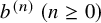 from [Reference Berman and WangBW18c]. This coincidence is the essence of our next main theorem; see Theorem 4.23. For the statement, let
$K_0(\mathbf {NB}_t)$
 be the split Grothendieck ring of the monoidal category of finitely generated projective graded
$\mathbf {NB}_t$
 -modules. This is a
$\mathbb {Z}[q,q^{-1}]$
 -algebra, with the action of q arising from the grading shift functor.
Theorem B. There is a unique
$\mathbb {Z}[q,q^{-1}]$
 -algebra isomorphism

intertwining the endomorphism of
$K_0(\mathbf {NB}_t)$
 induced by the endofunctor B with the endomorphism of
${{}_{\mathbb {Z}}}{\mathrm U}_t^{\imath }$
 defined by multiplication by the generator b of the iquantum group. For any
$n \geq 0$
 ,
$\kappa _t$
 maps the isomorphism class of the indecomposable projective module
$P(n)$
 to the icanonical basis element
$b^{(n)}$
 .
Under the isomorphism of Theorem B, the nondegenerate symmetric bilinear form
$(\cdot ,\cdot )^\imath $
 on
${{}_{\mathbb {Z}}}{\mathrm U}_t^{\imath }$
 constructed in [Reference Bao and WangBW18a] is equal (after twisting with the bar involution to make it sesquilinear in the appropriate sense, and some rescaling) to the Cartan form on
$K_0(\mathbf {NB}_t)$
 . The proof of this depends ultimately on the basis theorem for
$\mathbf {NB}_t$
 from [Reference Brundan, Wang and WebsterBWW24] together with some combinatorics of chord diagrams which is of independent interest; see Lemma 2.4, Corollary 2.6, and Theorem 3.7.
The remaining results in the article rely on the observation that the category of graded
$\mathbf {NB}_t$
 -modules has some useful additional structure: it is an affine lowest weight category in a suitably generalized sense. In particular, there are certain graded
$\mathbf {NB}_t$
 -modules
$\Delta (n)$
 ,
$\nabla (n)$
 ,
$\bar \Delta (n)$
 , and
$\bar \nabla (n)$
 , the standard, costandard, proper standard modules, and proper costandard modules, all of which are equipped with explicit bases. The proper standard module
$\bar \Delta (n)$
 has a unique irreducible quotient denoted
$L(n)$
 , which is also the unique irreducible submodule of
$\bar \nabla (n)$
 . The modules
$L(n)\:(n \geq 0)$
 give a complete set of graded irreducible
$\mathbf {NB}_t$
 -modules up to isomorphism and grading shift. There is a graded analog of the usual BGG reciprocity identifying certain standard filtration multiplicities
$(P(n):\Delta (m))_q$
 with the graded decomposition multiplicities
$[\bar \Delta (m):L(n)]_q$
 ; see Theorem 5.6. These assertions follow from an application of the general machinery of graded triangular bases developed in [Reference BrundanBru25] – the nil-Brauer category is a perfect example for this theory.
The minimal standard modules
$\Delta (0)$
 and
$\Delta (1)$
 are projective and therefore coincide with
$P(0)$
 and
$P(1)$
 , respectively, but after that the two families of modules diverge. At the decategorified level, the standard modules
$\Delta (n)$
 and costandard modules
$\nabla (n)$
 correspond to the standard basis
$\delta _n\:(n \geq 0)$
 and the costandard basis
 for
${\mathrm U}^{\imath }$
 , both of which are introduced in Section 2. These two bases are interchanged by the bar involution, and the costandard basis is an orthogonal basis with respect to the form
$(\cdot ,\cdot )^\imath $
 . The standard basis elements satisfy the following recurrence relation:

interpreting
$\delta _{-1}$
 as
$0$
 . This should be compared with the following theorem describing the effect of the endofunctor B on a standard module:
Theorem C. For
$n \geq 0$
 , there is a short exact sequence of graded
$\mathbf {NB}_t$
 -modules

In the first term, q denotes the upward grading shift functor, and this term should be interpreted as 0 in case
$n=0$
 .
An interesting feature of Theorem C is the presence of the infinite direct sum in the first term of the short exact sequence – the finitely generated
$\mathbf {NB}_t$
 -modules
$B \Delta (n)\:(n> 0)$
 are not Noetherian. This corresponds to the fact that the PBW basis
$\delta _n\:(n \geq 0)$
 is a basis for
${\mathrm U}^{\imath }$
 over
$\mathbb {Q}(q)$
 , but not for
${{}_{\mathbb {Z}}}{\mathrm U}_t^{\imath }$
 over
$\mathbb {Z}[q,q^{-1}]$
 . Theorem C is proved in Theorem 5.14 in the main body of the text. There is also a parallel result for proper standard modules; see Theorem 5.15.
For closed formulae for the transition matrices between the bases
$b^{(m)}\:(m \geq 0)$
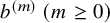 and
$\delta _n\:(n\geq 0)$
 , see Theorem 2.7. Translating to representation theory and using BGG reciprocity, we obtain the following explicit formula for graded decomposition numbers:
Theorem D. The irreducible subquotients of the proper standard module
$\bar \Delta (n)\:(n \geq 0)$
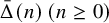 are isomorphic (up to grading shifts) to
$L(n+2m)$
 for
$m \geq 0$
 with

To formulate one more such combinatorial result, for a finitely generated graded
$\mathbf {NB}_t$
 -module V, its graded character is the series

where
$\chi $
 is a formal variable and
$\dim _q(1_n V) \in \mathbb {N}(\!( q )\!)$
 is the graded dimension of the graded vector space obtained by evaluating the functor V on the nth tensor power of the generating object B.
Theorem E. For
$n \geq 0$
 , we have that

Finally, we also prove branching rules which give complete information about the structure of the modules
$B L(n)\:(n \geq 0)$
 ; see Theorem 5.18. Except in the case that
$n=t=0$
 (when it is zero), these branching rules show that
$B L(n)$
 is a self-dual uniserial module with irreducible socle and cosocle isomorphic (up to appropriate grading shifts) to
$L(n-1)$
 if
$n \equiv t{\:\left (\mathrm {mod}\ 2\right )}$
 or to
$L(n+1)$
 if
$n \not \equiv t {\:\left (\mathrm {mod}\ 2\right )}$
 . Moreover,

where
$\beta (n) = n$
 if
$n \equiv t {\:\left (\mathrm {mod}\ 2\right )}$
 or
$n+1$
 if
$n \not \equiv t{\:\left (\mathrm {mod}\ 2\right )}$
 . The combinatorics arising here is the same as the combinatorics of the underlying icrystal basis described in [Reference WatanabeWat23, Ex. 4.1.4].
General conventions. Throughout the article,
$t \in \{0,1\}$
 will be a fixed parameter. Given also
$n \in \mathbb {N}$
 , we use the shorthand
$\delta _{n \equiv t}$
 to denote 1 if
$n \equiv t{\:\left (\mathrm {mod}\ 2\right )}$
 or 0 otherwise. Similarly,
$\delta _{n \not \equiv t}$
 denotes 1 if
$n \not \equiv t{\:\left (\mathrm {mod}\ 2\right )}$
 or 0 otherwise. We write
$S_n$
 for the symmetric group on n letters. Let
$s_i \in S_n$
 be the simple transposition
$(i\:\:i\!+\!1)$
 , let
$\ell :S_n \rightarrow \mathbb {N}$
 be the associated length function, and let
$w_n$
 be the longest element of
$S_n$
 . We denote the category of graded vector spaces over the field
$\Bbbk $
 by
$\mathbf {gVec}$
 , using q for the upward grading shift functor. So, for a graded vector space
$V=\bigoplus _{d \in \mathbb {Z}} V_d$
 , its grading shift
$qV$
 is the same underlying vector space with new grading defined via
$(q V)_d := V_{d-1}$
 for each
$d \in \mathbb {Z}$
 . For a graded vector space
$V = \bigoplus _{d \in \mathbb {Z}} V_d$
 with finite-dimensional graded pieces, we define its graded dimension to be

For any formal series
$f(q) = \sum _{d \in \mathbb {Z}} a_d q^d$
 with each
$a_d \in \mathbb {N}$
 , we write
$V^{\oplus f(q)}$
 for
$\bigoplus _{d \in \mathbb {Z}} q^d V^{\oplus a_d}$
 . Also
$\overline {f(q)}$
 denotes
$f(q^{-1})$
 .
2 Bases of the split iquantum group of rank one
In this section, we recall some basic facts about the split iquantum group of rank 1 following [Reference Bao and WangBW18b, Reference Berman and WangBW18c]. Then we introduce a new PBW-type basis, and derive combinatorial formulae for various transition matrices, including between the PBW basis and the icanonical basis. For all of this, we work over the field
$\mathbb {Q}(q)$
 for an indeterminate q. We write
$[n]$
 for the quantum integer
$\frac {q^n-q^{-n}}{q-q^{-1}}$
 ,
$[n]!$
 for the quantum factorial, and
$\genfrac {[}{]}{0pt}{}{n}{r}:=[n][n-1]\cdots [n-r+1] / [r]!$
 . The word antilinear always means with respect to the bar involution
$-:\mathbb {Q}(q)\rightarrow \mathbb {Q}(q)$
 that is the field automorphism taking q to
$q^{-1}$
 . We denote the limit of a convergent sequence
$(f_\lambda )_{\lambda \geq 0}$
 in
$\mathbb {Q}(\!( q^{-1} )\!)$
 by
$\lim _{\lambda \rightarrow \infty } f_\lambda $
 .
2.1 Quantum groups
Our general conventions for quantum groups are the same as in [Reference LusztigLus10], except that we write q in place of Lusztig’s v. Let
$\mathbf {f}$
 be the polynomial algebra over
$\mathbb {Q}(q)$
 generated by one element
$\theta $
 . We write
$\theta ^{(n)}$
 for the divided power
$\theta ^n / [n]!$
 . This is a fixed point for the bar involution
$\psi :\mathbf {f} \rightarrow \mathbf {f}$
 , which is the antilinear involution defined from
$\psi (\theta ) := \theta $
 . Let
$(\cdot ,\cdot ):\mathbf {f} \times \mathbf {f} \rightarrow \mathbb {Q}(q)$
 be the nondegenerate symmetric bilinear form from [Reference LusztigLus10, Sec. 1.2.5]. It satisfies

for
$m, n\geq 0$
 . Let
$R:\mathbf {f}\rightarrow \mathbf {f}$
 be the linear map defined by

for
$n \geq 1$
 . This map arises naturally as the adjoint of left multiplication by
$\theta $
 : we have that

for all
$x,y \in \mathbf {f}$
 . Equivalently,
$R(x) = r(x) / (1-q^{-2})$
 where r is the map defined in either the first or the second paragraph of [Reference LusztigLus10, Sec. 1.2.13] (the two maps coincide in rank one).
The quantum group
${\mathrm U}={\mathrm U}_q(\mathfrak {sl}_2)$
 is the
$\mathbb {Q}(q)$
 -algebra with generators
$e, f, k, k^{-1}$
 satisfying the relations

Here, we have switched to using lower case for
$e,f$
 compared to [Reference LusztigLus10] so that we can use the upper case letters
$E, F$
 for corresponding functors in categorification. The subalgebras of
${\mathrm U}$
 generated by f and by e are denoted
${\mathrm U}^-$
 and
${\mathrm U}^+$
 , respectively. Both are isomorphic to
$\mathbf {f}$
 via the maps
$\mathbf {f} \rightarrow {\mathrm U}^+, x \mapsto x^+$
 and
$\mathbf {f} \rightarrow {\mathrm U}^-, x \mapsto x^-$
 defined so that
$\theta ^+ := e$
 and
$\theta ^- := f$
 . The divided powers
$e^{(n)} := e^n / [n]!$
 and
$f^{(n)} := f^n / [n]!$
 are the images of
$\theta ^{(n)}$
 under these maps. There are various useful symmetries:
-
• Let $\psi :{\mathrm U} \rightarrow {\mathrm U}$
 be the usual bar involution on
${\mathrm U}$
, that is, the antilinear algebra involution that fixes e and f and takes k to
$k^{-1}$
.
-
• Let $\rho :{\mathrm U} \rightarrow {\mathrm U}$
be the linear algebra antiinvolution such that
$\rho (k) = k$
,
$\rho (e) = q kf$
,
$\rho (f) = q^{-1} e k^{-1}$
.


By [Reference LusztigLus10, Prop. 3.1.6(b)] (or an easy induction exercise using (2.2)), we have that

for any
$x \in \mathbf {f}$
 .
We denote the irreducible
${\mathrm U}$
 -module of highest weight
$\lambda \in \mathbb {N}$
 by
$V(\lambda )$
 . This is generated by a vector
$\eta _\lambda $
 such that
$e \eta _\lambda = 0$
 and
$k \eta _\lambda = q^\lambda \eta _\lambda $
 . There is an antilinear involution
$\psi _\lambda :V(\lambda )\rightarrow V(\lambda )$
 such that
$\psi _\lambda (\eta _\lambda ) = \eta _\lambda $
 and
$\psi _\lambda (uv) = \psi (u) \psi _\lambda (v)$
 for
$u \in {\mathrm U}, v \in V(\lambda )$
 . Also let
$(\cdot ,\cdot )_\lambda :V(\lambda )\times V(\lambda )\rightarrow \mathbb {Q}(q)$
 be the unique nondegenerate symmetric bilinear form on
$V(\lambda )$
 such that

for
$u \in {\mathrm U}, v_1,v_2 \in V(\lambda )$
 . The form
$(\cdot ,\cdot )$
 on
$\mathbf {f}$
 can be recovered from these forms on the modules
$V(\lambda )$
 since we have that

for all
$x,y \in \mathbf {f}$
 by a special case of [Reference LusztigLus10, Prop. 19.3.7]. The vectors
$f^{(n)} \eta _\lambda \:(0 \leq n \leq \lambda )$
 give the canonical basis for
$V(\lambda )$
 . In fact, they give a basis for an integral form
${{}_{\mathbb {Z}}}V(\lambda )$
 over
${\mathbb {Z}[q,q^{-1}]}$
 . The antiinvolution
$\psi _\lambda $
 restricts to an antilinear involution of
${{}_{\mathbb {Z}}}V(\lambda )$
 , and the values of the form
$(\cdot ,\cdot )_\lambda $
 on elements of
${{}_{\mathbb {Z}}}V(\lambda )$
 lie in
$\mathbb {Z}[q,q^{-1}]$
 .
For the purposes of categorification, one usually replaces
${\mathrm U}$
 by its modified form
$\dot {\mathrm U}$
 , which is a locally unital algebra
$\dot {\mathrm U} = \bigoplus _{\lambda ,\mu \in \mathbb {Z}} 1_\mu \dot {\mathrm U} 1_\lambda $
 with a distinguished system
$1_\lambda (\lambda \in \mathbb {Z})$
 of mutually orthogonal idempotents replacing the diagonal generators
$k, k^{-1}$
 . The relationship between
${\mathrm U}$
 and
$\dot {\mathrm U}$
 can be expressed either by saying that
$\dot {\mathrm U}$
 is a
$({\mathrm U},{\mathrm U})$
 -bimodule, or that
${\mathrm U}$
 embeds into the completion of
$\dot {\mathrm U}$
 consisting of matrices
$(a_{\mu ,\lambda })_{\lambda ,\mu \in \mathbb {Z}} \in \prod _{\lambda ,\mu \in \mathbb {Z}} 1_\mu \dot {\mathrm U} 1_\lambda $
 such that there are only finitely many nonzero entries in each row and column. The element
$k \in {\mathrm U}$
 corresponds to the diagonal matrix with
$q^\lambda 1_\lambda $
 as its
$\lambda $
 th diagonal entry, while
$e,f \in {\mathrm U}$
 are identified with the matrices whose only nonzero entries are
$1_{\lambda +2} e 1_\lambda \:(\lambda \in \mathbb {Z})$
 and
$1_{\lambda } f 1_{\lambda +2}\:(\lambda \in \mathbb {Z})$
 , respectively.
2.2 The iquantum group and its standard/costandard bases
The iquantum group
${\mathrm U}^\imath (\mathfrak {sl}_2)$
 is the subalgebra
${\mathrm U}^{\imath }$
 of
${\mathrm U}$
 generated by

As an algebra,
${\mathrm U}^{\imath }$
 is uninteresting since it is the free
$\mathbb {Q}(q)$
 -algebra on b. However, it is an interesting coideal subalgebra of
${\mathrm U}$
 for an appropriate choice of comultiplication.
The symmetry
$\rho $
 of
${\mathrm U}$
 restricts to a linear antiinvolution
$\rho :{\mathrm U}^{\imath }\rightarrow {\mathrm U}^{\imath }$
 with
$\rho (b) = b$
 . Also, the bar involution
$\psi ^\imath :{\mathrm U}^{\imath }\rightarrow {\mathrm U}^{\imath }$
 is the unique antilinear involution such that
$\psi ^\imath (b) = b$
 . We stress a key point:
$\psi ^\imath $
 is not the restriction of the bar involution
$\psi $
 on
${\mathrm U}$
 ; indeed, the latter does not leave
${\mathrm U}^{\imath }$
 invariant. For
$\lambda \in \mathbb {N}$
 , there is a unique antilinear involution
$\psi _\lambda ^\imath :V(\lambda )\rightarrow V(\lambda )$
 such that

for all
$u \in {\mathrm U}^{\imath }, v \in V(\lambda )$
 ; see [Reference Bao and WangBW18b, Cor. 3.11] and [Reference Bao and WangBW18a, Prop. 5.1]. Also, by [Reference Bao and WangBW18a, Lem. 6.25], there is a symmetric bilinear form
$(\cdot ,\cdot )^\imath : {\mathrm U}^{\imath }\times {\mathrm U}^{\imath } \rightarrow \mathbb {Q}(q)$
 such that

for all
$u_1,u_2 \in {\mathrm U}^{\imath }$
 . From (2.5), we get that

for any
$u_1,u_2 \in {\mathrm U}^{\imath }$
 . In [Reference Bao and WangBW18a, Th. 6.27], it is shown that
$(\cdot ,\cdot )^\imath $
 is nondegenerate. This also follows from the following theorem together with the nondegeneracy of the form
$(\cdot ,\cdot )^-$
 on
${\mathrm U}^-$
 .
Theorem 2.1. There is a unique isomorphism of
$\mathbb {Q}(q)$
 -vector spaces
$\jmath :{\mathrm U}^{\imath } \stackrel {\sim }{\rightarrow } \mathbf {f}$
 such that

for all
$u \in {\mathrm U}^{\imath }$
 and
$x \in \mathbf {f}$
 . Moreover, the following hold for
$u,u_1,u_2 \in {\mathrm U}^{\imath }$
 :
-
1. $\jmath (bu) = \theta \jmath (u) + R(\jmath (u))$
. -
2. $(u_1,u_2)^\imath = \big (\jmath (u_1), \jmath (u_2)\big )$
.


Proof. Uniqueness of a linear map
$\jmath $
 satisfying (2.11) follows easily from the nondegeneracy of the form
$(\cdot ,\cdot )$
 . To prove existence, we can assume that u is a power of b and proceed by induction on degree. Let
$\jmath (1) := 1$
 , which clearly satisfies (2.11) for all
$x \in \mathbf {f}$
 . Now assume for some
$u \in {\mathrm U}^{\imath }$
 that
$\jmath (u)$
 satisfying (2.11) for all x has been constructed inductively, and consider
$\jmath (bu)$
 . Using (2.5) and the identity (2.4) multiplied on the left by
$q k^{-1}$
 , we have that

So
$\jmath (bu) := \theta \jmath (u) + R(\jmath (u))$
 satisfies (2.11). This proves the existence of a linear map
$\jmath $
 satisfying (2.11), and at the same time we have established (1). To see that
$\jmath $
 is a linear isomorphism, it follows easily from (1) that
$\jmath (b^n)$
 is a monic polynomial of degree n in
$\theta $
 . Since
${\mathrm U}^{\imath }$
 and
$\mathbf {f}$
 are free on b and on
$\theta $
 , respectively, it is now clear that
$\jmath $
 is an isomorphism.
It remains to prove (2). By the definition (2.9) and (2.11), we need to show that

for all
$u_1,u_2 \in {\mathrm U}^{\imath }$
 . Note that the limit on the left hand side exists by what we have proved so far. We assume that
$u_2$
 is a power of b and proceed by induction on its degree. The base case
$u_2 = 1$
 is clear. Now assume the result has been proved for all
$u_1$
 and some
$u_2$
 , and consider
$b u_2$
 . Using (1), we have that

Applying Theorem 2.1, we let
 be the unique element such that
 . The elements
 give a basis for
${\mathrm U}^{\imath }$
 , which we call the costandard basis. From Theorem 2.1(2) and (2.1), we get that

for
$m,n\geq 0$
 . Thus, the costandard basis is an orthogonal basis. The following recurrence relation is easily deduced using Theorem 2.1(1) and (2.2):

for
$n \geq 0$
 , interpreting
 as
$0$
 . Applying the bar involution
$\psi ^\imath $
 to the costandard basis gives another basis
 for
${\mathrm U}^{\imath }$
 which we call the standard basis. It satisfies the recurrence

Despite only differing by an application of the bar involution, we generally prefer to work with
$\delta _n$
 , although
 has the advantage of being an orthogonal basis.
Remark 2.2. The linear isomorphism in Theorem 2.1 is analogous to the isomorphism
${\mathrm U}^+\otimes {\mathrm U}^- \cong \dot {\mathrm U} 1_\zeta $
 in [Reference WangWan25, Theorem 2.8]. The costandard basis for
${\mathrm U}^{\imath }$
 with the orthogonality property (2.12) is analogous to the PBW bases for modified quantum groups of finite type constructed in [Reference WangWan25].
2.3 Combinatorics of chord diagrams
Next, we investigate the rational functions
$w_{m,n}(q) \in \mathbb {Q}(q)$
 defined from the expansion

One reason to be interested in these is that

for any
$m,n \geq 0$
 .
Lemma 2.3. For
$0 \leq n \leq m$
 , we have that

interpreting
$w_{m,n}(q)$
 as 0 if
$n < 0$
 or
$n> m$
 .
Proof. Applying
$\jmath $
 to
 gives that
$\jmath (b^m) = \sum _{n=0}^m w_{m,n}(q) \theta ^{(n)}$
 . Thus,
$w_{m,n}(q)$
 is the
$\theta ^{(n)}$
 -coefficient of
$\jmath (b^m)$
 . Suppose that
$m \geq 1$
 . By Theorem 2.1(1), we have that
$\jmath (b^{m}) = \theta \jmath (b^{m-1}) + R(\jmath (b^{m-1}))$
 . Then we observe using (2.2) that the right hand side equals

From this, we see that the coefficient
$w_{m,n}(q)$
 of
$\theta ^{(n)}$
 in
$\jmath (b^m)$
 satisfies the recurrence relation in the statement of the lemma.
We are going to give an elementary combinatorial interpretation of
$w_{m,n}(q)$
 in terms of certain chord diagrams with n chords tethered to a fixed basepoint and
$f=(m-n)/2$
 free chords. The notion of a chord diagram is quite standard and we will not give a formal definition, but note in our setup that a pair of chords cannot intersect twice, and a chord cannot have both ends tethered. The following is an example of a chord diagram with
$n=3$
 tethered chords,
$f=4$
 free chords, and
$c=11$
 crossings:

The three tethered chords are the ones attached to the basepoint. We have also numbered the free endpoints of the tethered chords in order going clockwise around the circle. Here is one more example with
$n=4, f=3$
 , and
$c=5$
 :

In a chord diagram with f free and n tethered chords, the maximum possible number of crossings is
$nf+\frac {1}{2} f(f-1)$
 . Counting chord diagrams up to planar isotopy fixing the basepoint, let
$N(f,n,c)$
 be the number of chord diagrams with f free chords, n tethered chords, and c crossings, and

be the resulting generating function. We obviously have that
$T_{0,n}(q) = 1$
 , and
$T_{1,n}(q) = (n+1)+nq + (n-1)q^2+\cdots + q^n$
 . Other examples:
$T_{2,0}(q) = 2+q$
 and
$T_{3,0}(q) = 5+6q+3q^2+q^3$
 . Note also that
$T_{f,n}(1) = \binom {2f+n}{n} (2f-1)!!$
 (here,
$n!!$
 denotes the double factorial defined recursively by
$n!!=n\cdot (n-2)!!$
 and
$0!!= (-1)!!=1$
 ). Let
$\{n\}$
 be the classical q-integer
$1+q+q^2+\cdots +q^{n-1}$
 .
Lemma 2.4. The generating function
$T_{f,n}(q)$
 satisfies the recurrence relation

interpreting
$T_{f,n}(q)$
 as 0 if n or f is negative.
Proof. It is clear that
$T_{0,0}(q) = 1$
 . Now suppose that
$f+n> 0$
 . Let
$\mathrm {C}(f,n)$
 be the set of chord diagrams with f free and n tethered chords. We are going to construct a set partition

Take a chord diagram
$D \in \mathrm {C}(f,n)$
 . Consider the chord x in D that has the nearest free endpoint to the basepoint measured in a clockwise direction around the circumference of the circle. There are two cases:
-
• If x is a tethered chord then we put D into the set $\overline {\mathrm {C}}(f,n)$
and let
$\theta (D) \in \mathrm {C}(f,n-1)$
be the chord diagram obtained from D by removing x. Note that
$\theta (D)$
has the same number of crossings as D. An example of this situation is given by (2.18); for this
$\theta (D)$
is -
• Otherwise, x is a free chord. Its furthest endpoint from the basepoint lies between the free endpoints of the ith and $(i+1)$
th tethered chords for some
$0 \leq i \leq n$
. We put D into the set
$\mathrm {C}_i(f,n)$
and let
$\theta _i(D) \in \mathrm {C}(f-1,n+1)$
be the chord diagram obtained from D by replacing x by a tethered chord y with the same furthest endpoint as x. Note that
$\theta _i(D)$
has i fewer crossings than D since y crosses i fewer tethered chords compared to x. An example is given by (2.17); for this, we have that
$i=2$
and
$\theta _2(D)$
is





We have now defined the partition of
$\mathrm {C}(f,n)$
 . It is also clear that
$\theta :\overline {\mathrm {C}}(f,n)\stackrel {\sim }{\rightarrow } \mathrm {C}(f,n-1)$
 and all
$\theta _i:\mathrm {C}_i(f,n) \stackrel {\sim }{\rightarrow } \mathrm {C}(f-1,n+1)$
 are bijections. The lemma follows by computing the generating function
$T_{f,n}(q)$
 using this partition to see that
$T_{f,n}(q) = T_{f,n-1}(q) + \sum _{i=0}^n q^i T_{f-1,n+1}(q)$
 .
Theorem 2.5. For
$0 \leq n \leq m$
 with
$n \equiv m{\:\left (\mathrm {mod}\ 2\right )}$
 , we have that

Proof. It is clear from Lemma 2.3 that
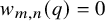
$w_{m,n}(q) = 0$
 if
$n \not \equiv m{\:\left (\mathrm {mod}\ 2\right )}$
 . Also using Lemma 2.3 it follows that the rational function
$\widetilde {T}_{f,n}(q)$
 defined from

satisfies the recurrence relation in Lemma 2.4. Hence,
$\widetilde {T}_{f,n}(q^2) = T_{f,n}(q^2)$
 and the result follows.
Corollary 2.6. The bilinear form
$(\cdot ,\cdot )^\imath $
 on
${\mathrm U}^{\imath }$
 satisfies

Proof. This follows from the theorem using also (2.16).
For example, Corollary 2.6 implies the following:

The generating function
$T_{f,0}(q)$
 for ordinary chord diagrams has been studied classically; for example, see [Reference RiordanRio75]. Our more general tethered chord diagrams will show up again in a slightly different guise later in the article; see Example 5.2.
2.4 The icanonical basis
So far we have not used the parameter
$t \in \{0,1\}$
 , but all subsequent results depend on it. To avoid notational confusion, it is helpful to appeal to the construction from [Reference Bao and WangBW18b, Chap. 4] and [Reference Bao and WangBW18a, Sec. 3.7], which shows that
${\mathrm U}^{\imath }$
 has a modified form
$\dot {\mathrm U}^{\imath } = \dot {\mathrm U}^{\imath } 1_{\bar 0} \oplus \dot {\mathrm U}^{\imath } 1_{\bar 1}$
 . We will denote the summands here simply by
${\mathrm U}_0^{\imath }$
 and
${\mathrm U}_1^{\imath }$
 since they are actually unital algebras. In fact, the map
${\mathrm U}^{\imath } \rightarrow \dot {\mathrm U}_t^{\imath }, u \mapsto u 1_t$
 is an algebra isomorphism. We use this to transport all of the results about
${\mathrm U}^{\imath }$
 established so far to
${\mathrm U}_t^{\imath }$
 , and work only with the latter from now on. In particular,
${\mathrm U}_t^{\imath }$
 is freely generated by
$b = b 1_t$
 , it has the symmetries
$\rho $
 and
$\psi ^\imath $
 fixing b as before, it possesses a bilinear form
$(\cdot ,\cdot )^\imath $
 as in (2.9), there is a linear isomorphism
$\jmath :{\mathrm U}_t^{\imath }\stackrel {\sim }{\rightarrow }\mathbf {f}$
 as in Theorem 2.1, and we have the standard basis
$\delta _n\:(n \geq 0)$
 for
${\mathrm U}_t^{\imath }$
 satisfying (2.14). However, one should have in mind that
${\mathrm U}_t^{\imath }$
 is a subalgebra not of the original quantum group
${\mathrm U}$
 but rather of the summand of the completion of
$\dot {\mathrm U}$
 consisting of matrices
$(a_{\mu ,\lambda })_{\mu ,\lambda \in \mathbb {Z}} \in \prod _{\lambda ,\mu \in \mathbb {Z}} 1_\mu \dot {\mathrm U} 1_\lambda $
 such that
$a_{\mu ,\lambda } = 0$
 if
$\lambda ,\mu \not \equiv t {\:\left (\mathrm {mod}\ 2\right )}$
 . This means that
${\mathrm U}_t^{\imath }$
 should only be allowed to act on
${\mathrm U}$
 -modules whose weights satisfy
$\lambda \equiv t {\:\left (\mathrm {mod}\ 2\right )}$
 . For example, the definition (2.9) of the form
$(\cdot ,\cdot )^\imath $
 on
${\mathrm U}_t^{\imath }$
 should really be written now as

for all
$u_1,u_2 \in {\mathrm U}_t^{\imath }$
 .
By the integrality properties from [Reference Bao and WangBW18b, Th. 4.18] and [Reference Bao and WangBW18a, Th. 5.3], the symmetry
$\psi _\lambda ^\imath $
 restricts to an antilinear involution on
${{}_{\mathbb {Z}}}V(\lambda )$
 . Applying [Reference Bao and WangBW18b, Th. 4.20] and [Reference Bao and WangBW18a, Th. 5.7], we define the icanonical basis for
$V(\lambda )$
 to be the unique
${\mathbb {Z}[q,q^{-1}]}$
 -basis
$b^{(n)} \eta _\lambda \:(0 \leq n \leq \lambda )$
 for
${{}_{\mathbb {Z}}}V(\lambda )$
 such that each
$b^{(n)} \eta _\lambda $
 is
$\psi _\lambda ^\imath $
 -invariant and

As the notation suggests, for
$\lambda \equiv t{\:\left (\mathrm {mod}\ 2\right )}$
 , the vector
$b^{(n)} \eta _\lambda $
 is obtained by applying an element
$b^{(n)} \in {\mathrm U}_t^{\imath }$
 to
$\eta _\lambda $
 . In fact, there is a unique element
$b^{(n)} \in {\mathrm U}_t^{\imath }\:(n \geq 0)$
 such that
$b^{(n)} \eta _\lambda $
 is the icanonical basis element of
$L(\lambda )$
 for all
$0\leq n \leq \lambda $
 with
$\lambda \equiv t {\:\left (\mathrm {mod}\ 2\right )}$
 ; see [Reference Bao and WangBW18b, Chap. 4] and [Reference Berman and WangBW18c, Th. 2.10, Th. 3.6]. The elements
$b^{(n)}\:(n \geq 0)$
 thus defined give a remarkable basis for
${\mathrm U}_t^{\imath }$
 again called the icanonical basis.
Closed formulae for the icanonical basis elements were worked out in [Reference Berman and WangBW18c] (see also [Reference Bao and WangBW18b]): for
$n\geq 0$
 , we have that

This is also known as the idivided power. It is straightforward to check from (2.23) that the icanonical basis satisfies the recurrence relation

for any
$n \geq 0$
 .
Theorem 2.7. For
$n \geq 0$
 , we have that


Proof. To prove the first formula, use (2.14) to verify that the expression on the right hand side satisfies the recurrence relation (2.24). Similarly, (2.26) follows by using (2.24) to verify that the expression on the right hand side satisfies the recurrence relation (2.14).
Corollary 2.8. The icanonical basis of
${\mathrm U}_t^{\imath }$
 is almost orthonormal in the sense that

for
$m,n \geq 0$
 .
Remark 2.9. Using (2.25), one can derive the following explicit formula for the pairings between icanonical basis elements:

for any
$m,n \geq 0$
 . This is 0 if
$m \not \equiv n{\:\left (\mathrm {mod}\ 2\right )}$
 .
The icanonical basis in fact gives a basis for an integral form
${{}_{\mathbb {Z}}}{\mathrm U}_t^{\imath }$
 of
${\mathrm U}_t^{\imath }$
 over
${\mathbb {Z}[q,q^{-1}]}$
 . Equivalently, we have that

from which one sees that
${{}_{\mathbb {Z}}}{\mathrm U}_t^{\imath }$
 is a
${\mathbb {Z}[q,q^{-1}]}$
 -subalgebra of
${\mathrm U}_t^{\imath }$
 . Since both
$\rho $
 and
$\psi ^\imath $
 fix each of the icanonical basis elements
$b^{(n)}$
 , they restrict to symmetries on
${{}_{\mathbb {Z}}}{\mathrm U}_t^{\imath }$
 . Also, the form on
${\mathrm U}_t^{\imath }$
 restricts to
$(\cdot ,\cdot )^\imath :{{}_{\mathbb {Z}}}{\mathrm U}_t^{\imath }\times {{}_{\mathbb {Z}}}{\mathrm U}_t^{\imath }\rightarrow \mathbb {Z}[q,q^{-1}]$
 . From (2.14), it is apparent that
$\delta _n \in {\mathrm U}_t^{\imath }$
 does not lie in the integral form.
2.5 The character ring
The character ring is the ring
 for a formal variable
$\chi $
 . It is natural to consider it from a representation-theoretic perspective (see subsection 5.4). We view
 as a left
${\mathrm U}_t^{\imath }$
 -module so that

and extending in the natural way to power series. We identify the character ring with the full linear dual
$\left ({\mathrm U}_t^{\imath }\right )^*$
 so that
$\sum _{n \geq 0} f_n(q) \chi ^n$
 is the function mapping
$b^n$
 to
$f_n(q)$
 . Thus, the topological basis for
 given by the monomials
$\chi ^n\:(n \geq 0)$
 is dual to the basis
$b^n\:(n \geq 0)$
 of
${\mathrm U}_t^{\imath }$
 . Then we let
$\ell _n, \bar \delta _n$
 , and
 be the unique elements of the character ring such that

for
$m,n \geq 0$
 . The topological bases
$\ell _n\:(n \geq 0)$
 ,
$\bar \delta _n\:(n \geq 0)$
 and
 for
 give the dual canonical basis, proper standard basis, and proper costandard basis, respectively.
There is a bar involution on the character ring, which is the antilinear map

This is compatible with the bar involution on
${\mathrm U}_t^{\imath }$
 in the sense that
$\bar \psi ^\imath (ug) = \psi ^\imath (u) \bar \psi ^\imath (g)$
 for
$u \in {\mathrm U}_t^{\imath }$
 and
 . Also, the bar involution on
 is related to the bar involution on
${\mathrm U}_t^{\imath }$
 by the formula

This follows easily from (2.29) as
$\psi ^\imath (b^n) = b^n$
 for each
$n \geq 0$
 . Using (2.30) and the definitions, it follows that the dual canonical basis elements
$\ell _n$
 are fixed by
$\bar \psi ^\imath $
 , and
 .
From Theorem 2.7, we get that


for
$n \geq 0$
 . Also the following recurrence relations may be deduced from (2.14) and (2.24):


for any
$n \geq 0$
 .
We proceed to derive explicit formulae for
$\bar \delta _n$
 and
$\ell _n$
 as formal series in
$\chi $
 .
Lemma 2.10. For
$n \geq 0$
 , we have that

Proof. By (2.15), we have that
$b^m = \sum _{n=0}^m w_{m,n}(q^{-1}) \delta _n$
 . Applying the function
$\bar \delta _n$
 to this equation, we deduce that the coefficient of
$\chi ^m$
 in the expansion of
$\bar \delta _n$
 is equal to
$w_{m,n}(q^{-1})$
 . It remains to apply Theorem 2.5.
Lemma 2.11.
$\ell _0 = \begin {cases} 1&\text {if }t=0\\ 1+\chi ^2+\chi ^4+\chi ^6+\cdots &\text {if }t=1. \end {cases}$

Proof. Suppose first that
$t=0$
 . We need to show that
$\ell _0(b^n) = \delta _{n,0}$
 for any
$n \geq 0$
 . This is clear for
$n=0$
 since
$b^0 = b^{(0)}$
 and
$\ell _0(b^{(0)}) = 1$
 . Also (2.23) shows that all
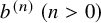
$b^{(n)}\:(n> 0)$
 are divisible by b, so we can use (2.23) to express
$b^n\:(n> 0)$
 as a linear combination of
$b^{(1)},\dots ,b^{(n)}$
 . This implies that
$\ell _0(b^n) = 0$
 for
$n> 0$
 as required.
Now suppose that
$t=1$
 . We need to show that
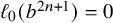
$\ell _0(b^{2n+1}) = 0$
 and
$\ell _0(b^{2n}) = 1$
 for
$n \geq 0$
 . By (2.23),
$b^{(2n+1)}$
 is a linear combination of
$b^{2m+1}$
 for
$0 \leq m \leq n$
 , and inverting obviously gives that
$b^{2n+1}$
 is a linear combination of
$b^{(2m+1)}$
 for
$0 \leq m \leq n$
 . This implies that
$\ell _0(b^{2n+1}) = 0$
 . Also, by (2.23) again,
$b^{(0)} = 1$
 and
$[2n][2n-1] b^{(2n)} = (b^2 - [2n-1]^2) b^{(2n-2)}$
 for
$n \geq 1$
 . Using this, one shows by induction on
$n\geq 0$
 that
$b^{2n} = a_n b^{(2n)} + \cdots + a_1 b^{(2)} + b^{(0)}$
 for some
$a_1,\dots ,a_n \in \mathbb {Q}(q)$
 . It follows that
$\ell _0(b^{2n}) = 1$
 .
Theorem 2.12. We have that

where
$\mathcal {P}_t(m\times n)$
 is the set of
$\alpha \in \mathbb {N}^m$
 with
$0 \leq \alpha _1 \leq \cdots \leq \alpha _m \leq n$
 and
$\alpha _i\not \equiv t {\:\left (\mathrm {mod}\ 2\right )}$
 for each i.
Proof. The second equality follows by expanding the product. To prove the first equality, we proceed by induction on n. The induction base follows from Lemma 2.11. For the induction step, take
$n> 0$
 . The constant term of
$\ell _n$
 is 0 since
$\ell _n(1) = \ell _n(b^{(0)}) = 0$
 so we have that
$b \ell _n = \ell _n / \chi $
 by (2.27). Suppose first that
$n\equiv t{\:\left (\mathrm {mod}\ 2\right )}$
 . Then (2.34) shows that

and we easily get done by induction in this case. When
$n\not \equiv t{\:\left (\mathrm {mod}\ 2\right )}$
 , (2.34) gives that

Hence,

and again the result follows by induction.
Corollary 2.13. For
$n \geq 0$
 , we have that

Proof. The coefficient of
$b^{(n-2m)}$
 in the expansion of
$b^n$
 is
$\ell _{n-2m}(b^n)$
 , that is, it is the
$\chi ^n$
 -coefficient of
$\ell _{n-2m}$
 . Now use Theorem 2.12.
3 The nil-Brauer category
For the remainder of the article, we will work over a field
$\Bbbk $
 of characteristic different from 2. All algebras, categories, functors, etc. will be assumed to be
$\Bbbk $
 -linear without further mention, and we reserve the symbol
$\otimes $
 for tensor products of vector spaces or algebras over
$\Bbbk $
 . By a graded category, graded monoidal category, graded functor, etc., we mean one that is enriched in the closed symmetric monoidal category
$\mathbf {gVec}$
 of graded vector spaces.
In this section, we first recall the definition of the nil-Brauer category
$\mathbf {NB}_t$
 and the crucial basis theorem for its morphism spaces from [Reference Brundan, Wang and WebsterBWW24]. Then we relate the graded dimensions of these spaces to the bilinear form
$(\cdot ,\cdot )^\imath $
 on the iquantum group
${\mathrm U}_t^{\imath }$
 . Finally, we discuss the center of
$\mathbf {NB}_t$
 , and prove a useful result about minimal polynomials.
3.1 Definition and basic properties
We use the usual string calculus for morphisms in strict monoidal categories; our general convention is that
$f \circ g$
 denotes composition of f drawn on top of g (“vertical composition”) and
$f \star g$
 denotes the tensor product of f drawn to the left of g (“horizontal composition”). We always draw string diagrams so that the underlying strings are smooth curves. Recall the following definition from [Reference Brundan, Wang and WebsterBWW24, Def. 2.1].
Definition 3.1. The nil-Brauer category
$\mathbf {NB}_t$
 is the strict graded monoidal category with one generating object B (whose identity endomorphism will be represented diagrammatically by the unlabeled string
 ) and four generating morphisms

subject to the following relations:


Remark 3.2. One source of motivation for Definition 3.1 is the expected compatibility of
$\mathbf {NB}_t$
 with the bilinear form
$(\cdot ,\cdot )^\imath $
 on
${\mathrm U}_t^{\imath }$
 , something which will be proved in general in Theorem 3.7. From this perspective, the formulae (2.21) suggest the existence of generators of the degrees specified in (3.1) and some of the basic relations. This is similar to Lauda’s approach to categorification of
${\mathrm U}_q(\mathfrak {sl}_2)$
 in [Reference LaudaLau10].
The following relations are easily derived from the defining relations in [Reference Brundan, Wang and WebsterBWW24, (2.6)–(2.8)]:


In view of the last relation from (3.4) and the first relation from (3.6), we can unambiguously denote the morphisms in these two equations by the “pitchforks”
 and
 , respectively. Together with the last relation of (3.3), it then follows that a string diagram with no dots can be deformed under planar isotopy without changing the morphism that it represents. This is not true in the presence of dots due to the sign in the last relations of (3.5) and (3.8) – there is a sign change whenever a dot slides across the critical point of a cup or cap.
The relations discussed so far imply that there are strict graded monoidal functors


Here, for a string diagram s we use
$s^{\updownarrow }$
 and
$s^{\leftrightarrow }$
 to denote its reflection in a horizontal or vertical axis, and
$\bullet (s)$
 denotes the total number of dots in the diagram. The category
$\mathbf {NB}_t$
 is pivotal with duality functor
${\scriptstyle \mathrm {D}} := {\scriptstyle \mathrm {R}} \circ {\scriptstyle \mathrm {T}} = {\scriptstyle \mathrm {T}} \circ {\scriptstyle \mathrm {R}}$
 , which rotates a string diagram s through
$180^\circ $
 then scales by
$(-1)^{\bullet (s)}$
 .
3.2 Generating functions for dots and bubbles
Next we recall the generating function formalism from [Reference Brundan, Wang and WebsterBWW24, Sec. 2]. We denote the rth power of
 under vertical composition simply by labeling the dot with r. More generally, given a polynomial
$f(x) = \sum _{r\geq 0} c_r x^r \in \Bbbk [x]$
 and a dot in some string diagram s, we denote

by attaching what we call a pin to the dot, labeling the node at the head of the pin by
$f(x)$
 :

In the drawing of a pin, the arm and the head of the pin can be moved freely around larger diagrams so long as the dot at the pointy end stays put – these are not part of the string calculus. More generally,
$f(x)$
 here could be a polynomial with coefficients in the algebra
$\Bbbk (\!( u^{-1} )\!)$
 of formal Laurent series in an indeterminate
$u^{-1}$
 ; then the string s decorated with a pin labeled
$f(x)$
 defines a generating function of morphisms.
We will use the following shorthands for the generating functions of [Reference Brundan, Wang and WebsterBWW24, (2.14)–(2.15)]:


The notation here is motivated by the following standard trick: for any
$f(x) \in \Bbbk [x]$
 , we have that

where
$[-]_{u^r}$
 denotes the
$u^r$
 -coefficient of the formal Laurent series inside the brackets. These identities follow by using linearity to reduce to the case that
$f(x) = x^n$
 for
$n \geq 0$
 , then explicitly computing coefficients on both sides. As we do with ordinary dots, we denote the nth power of one of these “dot generating functions” by labeling them also by n. This makes sense for any
$n \in \mathbb {Z}$
 since we have by the definitions that

The endomorphisms (3.12) and (3.13) obviously commute with each other and all other pins. Note also that
${\scriptstyle \mathrm {T}}$
 and
${\scriptstyle \mathrm {R}}$
 satisfy

Another useful trick is to apply the substitution
$u \mapsto -u$
 ; this interchanges
 and
 .
It is clear from the last relation in (3.4) that
 and similarly for cups; hence, we have that

Further useful relations involving these generating functions are

These are also noted in [Reference Brundan, Wang and WebsterBWW24, (2.19)–(2.20)]. Equating the coefficients of
$u^{-n-1}$
 , we obtain


Now consider the “dotted bubble generating function”

This is often useful, but even more important will be the renormalization

Its
$u^{-r}$
 -coefficients
$\mathbb {O}_r$
 are given explicitly by

for
$r \geq 1$
 . Note also by (3.15) and (3.16) that
$\mathbb {O}(u)$
 is invariant under
${\scriptstyle \mathrm {R}}$
 and
${\scriptstyle \mathrm {T}}$
 .
Theorem 3.3 [Reference Brundan, Wang and WebsterBWW24, Th. 2.5].
The following relations hold in
$\mathbf {NB}_t$
 :


Corollary 3.4. The following relations hold in
$\mathbf {NB}_t$
 :


Proof. The first equality follows from (3.23) and the definition (3.21). The others follow by applying
${\scriptstyle \mathrm {R}}$
 or using the substitution
$u \mapsto -u$
 .
Corollary 3.5. For
$n \geq 0$
 , we have that

Proof. This follows by equating the coefficients of
$u^{-n-1}$
 in the first equation from (3.27).
3.3 The basis theorem
Let
$\Lambda $
 be the graded algebra of symmetric functions over
$\Bbbk $
 . Adopting standard notation, this is freely generated either by the elementary symmetric functions
$e_r\:(r> 0)$
 or by the complete symmetric functions
$h_r\:(r> 0)$
 ; our convention for the grading puts these in degree
$2r$
 . The two families of generators are related by the identity

where

are the corresponding generating functions, and
$e_0 = h_0 = 1$
 by convention. It is also convenient to interpret
$e_r$
 and
$h_r$
 as
$0$
 when
$r < 0$
 .
Following [Reference MacdonaldMac15, Ch. III, Sec. 8], we define a power series
 and elements
$q_r\;(r \geq 0)$
 of
$\Lambda $
 so that

By (3.29), we have that

Equivalently,
$q_0 = 1$
 and

for
$r \geq 1$
 ; cf. [Reference MacdonaldMac15, (III.8.2’)]. As with
$e_r$
 and
$h_r$
 , we adopt the convention that
$q_r = 0$
 for
$r < 0$
 .
The graded subalgebra of
$\Lambda $
 generated by all
$q_r\:(r \geq 0)$
 is denoted
$\Gamma $
 . As explained in [Reference MacdonaldMac15],
$\Gamma $
 is freely generated by
$q_1,q_3,q_5,\dots $
 (and it has a distinguished basis given by the Schur Q-functions
$Q_\lambda $
 indexed by all strict partitions). It follows that
$\Gamma $
 is generated by the elements
$q_r\:(r \geq 0)$
 subject only to the relations (3.32). Hence, (3.25) is all that is needed to establish the existence of a graded algebra homomorphism

By [Reference Brundan, Wang and WebsterBWW24, Cor. 5.4], this is actually an isomorphism.
Now we recall the basis theorem for morphism spaces in
$\mathbf {NB}_t$
 , which is the main result of [Reference Brundan, Wang and WebsterBWW24]. For
$m, n \geq 0$
 , any morphism
$f:B^{\star n} \rightarrow B^{\star m}$
 is represented by a linear combination of
$m \times n$
 string diagrams, that is, string diagrams with m boundary points at the top and n boundary points at the bottom that are obtained by composing the generating morphisms from (3.1). It follows that
$ {\mathrm {Hom}}_{\mathbf {NB}_t}(B^{\star n}, B^{\star m})$
 is 0 unless
$m \equiv n {\:\left (\mathrm {mod}\ 2\right )}$
 . The individual strings in an
$m \times n$
 string diagram s are of four basic types: cups (with two boundary points on the top edge), caps (with two boundary points on the bottom edge), propagating strings (with one boundary point at the top and one at the bottom), and internal bubbles (no boundary points). We define an equivalence relation
$\sim $
 on the set of
$m \times n$
 string diagrams by declaring that
$s \sim s'$
 if their strings define the same matching on the set of
$m+n$
 boundary points. We say that s is reduced if the following properties hold:
-
• There are no internal bubbles.
-
• Propagating strings have no critical points ( $\!\! =$
points of slope 0). -
• Cups and caps each have exactly one critical point.
-
• There are no double crossings ( $\!\! =$
two different strings which cross each other at least twice).


These assumptions imply in particular that there are no self-intersections (
$=$
 crossings of a string with itself). Fix a set
$\overline {\mathrm {D}}(m\times n)$
 of representatives for the
$\sim $
 -equivalence classes of undotted reduced
$m \times n$
 string diagrams. The total number of such diagrams is
$(m+n-1)!!$
 if
$m \equiv n {\:\left (\mathrm {mod}\ 2\right )}$
 , and there are none otherwise. For each of these
$\sim $
 -equivalence class representatives, we also choose distinguished points in the interior of each of its strings that are away from points of intersection. Then let
$\mathrm {D}(m\times n)$
 be the set of all morphisms
$f:B^{\star n} \rightarrow B^{\star m}$
 which can be obtained by taking an element of
$\overline {\mathrm {D}}(m\times n)$
 then adding dots labeled by nonnegative multiplicities at each of the distinguished points on the strings.
Theorem 3.6 [Reference Brundan, Wang and WebsterBWW24, Th. 5.1].
Viewed as a graded
$\Gamma $
 -module so that
$p \in \Gamma $
 acts on
$f:B^{\star n}\rightarrow B^{\star m}$
 by
$f \cdot p := f \star \gamma _t(p)$
 , the space
$ {\mathrm {Hom}}_{\mathbf {NB}_t}(B^{\star n}, B^{\star m})$
 is free with basis
$\mathrm {D}(m\times n)$
 .
Now we can make the first significant connection between
$\mathbf {NB}_t$
 and the iquantum group. Recall the bilinear form
$(\cdot ,\cdot )^\imath :{\mathrm U}_t^{\imath } \times {\mathrm U}_t^{\imath } \rightarrow \mathbb {Q}(q)$
 from (2.22).
Theorem 3.7. For
$m,n \in \mathbb {N}$
 , we have that
$ {\mathrm {Hom}}_{\mathbf {NB}_t}(B^{\star n}, B^{\star m}) \cong \Gamma ^{\oplus \overline {(b^m, b^n)^\imath }}$
 as a graded
$\Gamma $
 -module.
Proof. We compare the explicit combinatorial formula for
$(b^m, b^n)^\imath $
 from Corollary 2.6 with the graded rank of
$ {\mathrm {Hom}}_{\mathbf {NB}_t}(B^{\star n}, B^{\star m})$
 as a free graded
$\Gamma $
 -module computed via Theorem 3.6. If
$m \not \equiv n {\:\left (\mathrm {mod}\ 2\right )}$
 then
$(b^m,b^n)^\imath = 0$
 and
$\mathrm {D}(m\times n)$
 is empty, and the result is clear. Now assume that
$m \equiv n {\:\left (\mathrm {mod}\ 2\right )}$
 and let
$f := (m+n)/2$
 . There is an obvious bijection between equivalence classes of
$m \times n$
 string diagrams and chord diagrams with f free chords and no tethered chords. This just arises by identifying the
$(m+n)$
 boundary points of strings in an
$m \times n$
 string diagram with the
$(m+n)$
 endpoints of chords in a chord diagram in some fixed way that preserves the clockwise ordering, then replacing strings by chords so that the underlying matching of these points is preserved. In a string diagram, each crossing is of degree
$-2$
 , so it contributes
$q^{-2}$
 to the graded rank. The dots placed at the f distinguished points produce the factor
$1 / (1-q^{2})^f$
 , this being
$\dim _{q} \Bbbk [x_1,\dots ,x_f]$
 with
$x_i$
 in degree 2. Recalling the definition of the generating function
$T_{f,0}(q)$
 from (2.19), we deduce that

which is
$\overline {(b^m,b^n)^\imath }$
 according to Corollary 2.6.
3.4 Central elements
Recall that the center
$Z(\mathbf {A})$
 of a category
$\mathbf {A}$
 means the algebra of endomorphisms of its identity endofunctor. Thus, elements of
$Z(\mathbf {NB}_t)$
 consist of tuples
$(z_n)_{n \geq 0}$
 for elements
$z_n \in {\mathrm {End}}_{\mathbf {NB}_t}(B^{\star n})$
 such that
$z_m \circ f = f \circ z_n$
 for all
$m,n \geq 0$
 and
$f \in {\mathrm {Hom}}_{\mathbf {NB}_t}(B^{\star n}, B^{\star m})$
 . In this subsection, we are going to use the dotted bubbles to construct many – conjecturally, all – elements of
$Z(\mathbf {NB}_t)$
 .
Since
 and
$2$
 is invertible in
$\Bbbk $
 , it makes sense to take the square roots
$\sqrt {\mathbb {O}(\pm u)}$
 ; we choose the ones that are positive in the sense that they again lie in
 . We have that
$\sqrt {\mathbb {O}(-u)} = \left (\sqrt {\mathbb {O}(u)}\right )^{-1}$
 by (3.25). Taking the square roots of both sides of (3.26), both of which lie in
 , we obtain

Let
$e_{r,n}, h_{r,n}, q_{r,n} \in \Bbbk [x_1,\dots ,x_n]^{S_n}$
 be the symmetric polynomials in n variables obtained by specializing the symmetric functions
$e_r, h_r, q_r$
 from (3.30) and (3.31). We have that

Moreover,

In the statement of the next theorem, for a polynomial
$f \in \Bbbk [x_1,\dots ,x_n]$
 , we use the notation
$f 1_n = 1_n f$
 to denote the endomorphism of
$B^{\star n}$
 defined by interpreting
$x_i$
 as
 , that is, the dot on the ith string.
Theorem 3.8. For any
$r \geq 0$
 , we have that
$\left (q_{r,n} 1_n\right )_{n \geq 0}\in Z(\mathbf {NB}_t)$
 .
Proof. We need to show that
$q_{r,m} 1_m \circ f = f \circ q_{r,n} 1_n$
 for any
$f \in {\mathrm {Hom}}_{\mathbf {NB}_t}\left (B^{\star n}, B^{\star m}\right )$
 . By (3.35), we have that

The result follows from this since the expression on the right hand side clearly has the desired property by the interchange law.
Corollary 3.9. Let
$p_{r,n} := \sum _{i=1}^n x_i^r \in \Bbbk [x_1,\dots ,x_n]^{S_n}$
 be the rth power sum. For any odd
$r \geq 1$
 , we have that
$(p_{r,n} 1_n)_{n \geq 0} \in Z(\mathbf {NB}_t)$
 .
Proof. It suffices to note that any odd power sum can be written as a polynomial in the symmetric polynomials
$q_{r,n}$
 . This can be proved by taking the logarithmic derivative of (3.37).
3.5 Cyclotomic quotients
In this subsection, the grading plays no role – we view
$\mathbf {NB}_t$
 simply as a strict
$\Bbbk $
 -linear monoidal category. Let
$\mathbf {V}$
 be a strict
$\mathbf {NB}_t$
 -module category. This means that
$\mathbf {V}$
 is a
$\Bbbk $
 -linear category, and we are given a strict
$\Bbbk $
 -linear monoidal functor
$\mu $
 from
$\mathbf {NB}_t$
 to the strict
$\Bbbk $
 -linear monoidal category
$\mathbf {End}_\Bbbk (\mathbf {V})$
 whose objects are
$\Bbbk $
 -linear endofunctors of
$\mathbf {V}$
 and whose morphisms are natural transformations. We denote the endofunctor
$\mu (B):\mathbf {V}\rightarrow \mathbf {V}$
 simply by B. The string calculus for monoidal categories extends to the module category
$\mathbf {V}$
 in the usual way. We will represent the identity endomorphism of an object V of
$\mathbf {V}$
 by the labeled string
 on the right hand boundary of the diagram. For a string diagram s representing a morphism in
$ {\mathrm {Hom}}_{\mathbf{NB}_{t}}(B^{\star n},B^{\star m})$
 , we represent the morphism
$\mu (s)_V:B^n V \rightarrow B^m V$
 diagrammatically by
 .
Let
$V \in \mathbf {V}$
 be any object. We write
$Z_V$
 for the center of its endomorphism algebra. Any dotted bubble evaluates to an element of
$Z_V$
 . In particular, the generating function
$\mathbb {O}(u)$
 for dotted bubbles from (3.21) evaluates to a power series
 . Let

be the
$\Bbbk $
 -algebra homomorphism mapping
$z \in Z_V$
 to
$B z : BV \rightarrow BV$
 and u to the endomorphism of
$BV$
 defined by the dot. We represent
$\theta _V(f(u))$
 diagrammatically by
 . The coefficients of
$f(x)$
 are elements of
$Z_V$
 which could be represented by coupons on the right-hand string, but we will not attempt to do that here. Let
$I_V := \ker \theta _V \unlhd Z_V[u]$
 .
Theorem 3.10. Let V be an object of an
$\mathbf {NB}_t$
 -module category
$\mathbf {V}$
 as above, and
$f(u) \in I_V$
 . The formal Laurent series
$f^*(u) := (-1)^t f(-u) \mathbb {O}_V(-u) \in Z_V(\!( u^{-1})\!)$
 is a polynomial in
$I_V$
 with the same constant term as
$f(u)$
 , and
$f^{**}(u) = f(u)$
 . Moreover,
$\tfrac {f(u)+f^*(u)}{2}$
 and
$\tfrac {f(u)-f^*(u)}{2u}$
 are
$*$
 -invariant elements of
$I_V$
 . Assuming in addition that
$f(u) \in I_V$
 is monic,

is a monic polynomial in
$I_V$
 with
$\deg g(u) = \deg f(u)$
 or
$\deg g(u) = \deg f(u)-1$
 in the two cases, such that
$\mathbb {O}_V(u) = (-1)^t g(-u) / g(u)$
 .
Proof. For
$r \geq 0$
 , we have that

Thus, for
$r \geq 0$
 , we have that
$\left [f^*(u)\right ]_{u^{-r}} =\left [f(-u)\right ]_{u^{-r}} = \delta _{r,0} f(0)$
 . This shows that
$f^*(u)$
 is a polynomial in
$Z_V[u]$
 with the same constant term as
$f(u)$
 . Also
$f^{**}(u) = f(u) \mathbb {O}_V(u)\mathbb {O}_V(-u)$
 , which equals
$f(u)$
 by (3.25).
Since
$f^*(u)$
 and
$f(u)$
 are polynomials with the same constant terms,
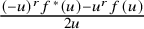
$\frac {(-u)^r f^*(u) - u^r f(u)}{2u}$
 is a polynomial in u for any
$r \geq 0$
 . So it is an element of
$Z_V[u]$
 . Its image under
$\theta _V$
 is

Thus, we have proved that
$\frac {(-u)^r f^*(u) - u^r f(u)}{2u} \in I_V$
 for any
$r \geq 0$
 . The
$r=0$
 and
$r=1$
 cases show that
$\tfrac {f(u)+f^*(u)}{2}$
 and
$\tfrac {f(u)-f^*(u)}{2u}$
 both belong to
$I_V$
 , which implies that
$f^*(u) \in I_V$
 . Moreover, it is easy to check using
$f^{**}(u) = f(u)$
 that both of these elements are
$*$
 -invariant.
Finally, we assume that
$f(u)$
 is monic and consider the two cases separately:
-
• If $\deg f(u) \equiv t {\:\left (\mathrm {mod}\ 2\right )}$
, then both
$f(u)$
and
$f^*(u)$
are monic, so
$g(u) := \frac {f(u) + f^*(u)}{2} \in I_V$
is monic of the same degree as
$f(u)$
. -
• If $\deg f(u) \not \equiv t {\:\left (\mathrm {mod}\ 2\right )}$
then both
$f(u)$
and
$-f^*(u)$
are monic, so
$g(u) := \frac {f(u)-f^*(u)}{2u} \in I_V$
is monic of one less degree than
$f(u)$
.








The equality
$g^*(u) = g(u)$
 means that
$(-1)^t g(-u) \mathbb {O}_V(-u) = g(u)$
 , so
$g(u) \mathbb {O}_V(u) = (-1)^t g(-u)$
 . Since
$g(u)$
 is monic, it is invertible in
$Z_V(\!( u^{-1})\!)$
 , and the final assertion of the theorem follows.
Some of the ideas in the proof of Theorem 3.10 were suggested by Anthropic’s Claude AI. In the first version of this paper, we were only able to prove the slightly weaker result in the following corollary, which is all that is needed later on in the article.
Corollary 3.11. Suppose that V is an object of
$\mathbf {V}$
 such that
$ {\mathrm {End}}_{\mathbf {V}}(V) = \Bbbk $
 and
$\dim {\mathrm {End}}_{\mathbf {V}}(B V) < \infty $
 . The ideal
$I_V$
 of the PID
$\Bbbk [u]$
 is nonzero, so it is generated by the unique monic polynomial
$m_V(u)$
 of smallest degree belonging to
$I_V$
 . Moreover,
$\deg m_V(u) \equiv t {\:\left (\mathrm {mod}\ 2\right )}$
 and
$\mathbb {O}_V(u) = (-1)^t m_V(-u) / m_V(u)$
 .
Proof. The kernel is nonzero since
$\theta _V$
 is a homomorphism from the infinite-dimensional algebra
$\Bbbk [u]$
 to
$ {\mathrm {End}}_{\mathbf {V}}(BV)$
 , which is finite dimensional. Now we apply Theorem 3.10 taking
$f(u) := m_V(u)$
 . If
$\deg m_V(u) \not \equiv t {\:\left (\mathrm {mod}\ 2\right )}$
 , the theorem shows that
$\frac {1}{2u}(m_V(u) - m_V^*(u))$
 is a monic polynomial in
$I_V$
 of smaller degree than
$m_V(u)$
 , which is a contradiction. Thus,
$\deg m_V(u) \equiv t {\:\left (\mathrm {mod}\ 2\right )}$
 . Now the theorem shows that
$g(u) := \frac {1}{2}(m_V(u)+m_V^*(u))$
 is a monic polynomial of the same degree as
$m_V(u)$
 . Since
$m_V(u)$
 is the unique monic polynomial in
$I_V$
 of this degree, it follows that
$g(u) = m_V(u)$
 . Consequently, the last part of Theorem 3.10 shows that
$\mathbb {O}_V(u) = (-1)^t m_V(-u) / m_V(u)$
 .
Remark 3.12. In this remark – not needed subsequently in the article – we briefly explain why Theorem 3.10 is significant. Suppose that
$l \geq 0$
 with
$l \equiv t {\:\left (\mathrm {mod}\ 2\right )}$
 . Let
$\Lambda _l := \Bbbk [x_1,\dots ,x_l]^{S_l}$
 be the algebra of symmetric polynomials and
$e_l(u) := (u-x_1)\cdots (u-x_l) \in \Lambda _l[u]$
 . Let
$\mathbf {cNB}_l$
 be the cyclotomic nil-Brauer category from [Reference Bodish, Brundan and EliasBBE26, Def. 2.11]. It is a strict
$\Bbbk $
 -linear monoidal category in its own right, but all that is important here is that
$\mathbf {cNB}_l$
 is a strict
$\mathbf {NB}_t$
 -module category. An equivalent way to formulate the definition of
$\mathbf {cNB}_l$
 is that it is the quotient of the
$\Lambda _l$
 -linear
$\mathbf {NB}_t$
 -module category
$\mathbf {NB}_t \otimes _\Bbbk \Lambda _l$
 by the
$\Lambda _l$
 -linear submodule category generated by the relations
$\mathbb {O}(u) = (-1)^t e_l(-u) / e_l(u)$
 and
 . Moreover, we have that
 . Indeed, it is easy to see from the definition that the canonical map
 is surjective, and
$\iota $
 is injective because its composition with the algebra homomorphism
 defined by the functor
$\Theta $
 from [Reference Bodish, Brundan and EliasBBE26, Th. 5.1] is the identity.
Now let
$V \in \mathbf {V}$
 be as above, and assume that
$\dim {\mathrm {End}}_{\mathbf {V}}(BV) < \infty $
 . This assumption ensures that there exist monic polynomials
$f(u) \in I_V$
 . Hence, by Theorem 3.10, there exists a monic polynomial
$g(u) \in I_V$
 such that
$l := \deg g(u) \equiv t {\:\left (\mathrm {mod}\ 2\right )}$
 and
$\mathbb {O}_V(u) = (-1)^t g(-u) / g(u)$
 . In view of the defining relations for
$\mathbf {cNB}_l$
 described in the previous paragraph, it follows that there is a unique morphism of strict
$\mathbf {NB}_t$
 -module categories
$\mathrm {ev}_V: \mathbf {cNB}_l \rightarrow \mathbf {V}$
 mapping the generating object
 of
$\mathbf {cNB}_l$
 to V and the polynomial
 to
$g(u) \in {\mathrm {End}}_{\mathbf {V}}(V)[u]$
 . This makes precise the idea that
$\mathbf {cNB}_l$
 is the universal cyclotomic quotient of
$\mathbf {NB}_t$
 of level l.
For a description of the Grothendieck group
$K_0(\mathbf {cNB}_l)$
 as a left
$K_0(\mathbf {NB}_t)$
 -module, see [Reference Bodish, Brundan and EliasBBE26].
4 Primitive idempotents
In this section, we work out the structure of the primitive homogeneous idempotents in
$\mathbf {NB}_t$
 and prove Theorems A and B. We continue to work over the field
$\Bbbk $
 of characteristic different from 2.
4.1 Extended graphical calculus
We begin by introducing some further diagrammatical shorthands in the spirit of the “thick calculus” of [Reference Khovanov, Lauda, Mackaay and StošićKLMS12]. We denote the tensor product
$|^{\star a}$
 of a strings by a single thick string labeled by a. A thick cup or cap labeled by a denotes that number of nested ordinary cups or caps (no crossings). Sometimes it is notationally convenient to be able to split thick strings into thinner ones or to merge thinner strings to obtain thicker ones: the diagrams

simply represent the identity morphisms
$B^{\star n} \rightarrow B^{\star a} \star B^{\star b}$
 and
$B^{\star a} \star B^{\star b} \rightarrow B^{\star n}$
 for
$a+b=n$
 . We will often omit a thickness label on a thick string when it can be inferred from others in the diagram.
For
$a+b=n$
 , the thick crossing

denotes the morphism
$B^{\star a} \star B^{\star b} \rightarrow B^{\star b} \star B^{\star a}$
 obtained by composing ordinary crossings according to a reduced expression for the longest of the minimal length
$S_n / (S_a \times S_b)$
 -coset representatives. We use a thick string decorated with a cross to denote the composition of thin crossings corresponding to a reduced expression for the longest element
$w_n$
 . For example:

When working with these morphisms, we will often make implicit use of various obvious consequences of the braid relations, such as

In view of the pitchfork relations, one can also draw this cross at the critical point of a thick cup or cap without there being any ambiguity as to the meaning:

We use a dot on a string of thickness n labeled by
$\alpha \in \mathbb {N}^n$
 to denote the tensor product of dots on ordinary strings labeled by the parts of
$\alpha $
 :

The n-tuples
$\rho _n := (n-1,n-2,\dots ,1,0) \in \mathbb {N}^n$
 and
$\varpi _{r,n} := (1,\dots ,1,0,\dots ,0) \in \mathbb {N}^n$
 with r entries equal to
$1$
 followed by
$(n-r)$
 entries equal to
$0$
 will appear often. To simplify notation, we allow the subscript n to be omitted in these when used to label a node on a string of thickness n:

Generalizing the notation (3.11), given a polynomial
$f= \sum _{\alpha \in \mathbb {N}^n} c_\alpha x_1^{\alpha _1} \cdots x_n^{\alpha _n} \in \Bbbk [x_1,\dots ,x_n]$
 , the pin

denotes the endomorphism
$f 1_n = 1_n f$
 of
$B^{\star n}$
 . Often this f will be the elementary symmetric polynomial
$e_{r,n} := \sum _{1 \leq i_1 < \cdots < i_r \leq n} x_{i_1} \cdots x_{i_r}$
 . Again, if this is pinned to a string of thickness n, we allow the subscript n to be dropped, writing simply

since the number n of variables in the elementary symmetric polynomial can be inferred from the thickness of the string.
Lemma 4.1. For
$0 \leq r \leq n$
 , we have that

Proof. The first equality is the well-known identity
$e_{r,n} = \sum _{s=0}^r (-1)^{r-s} x_{n+1}^{r-s}e_{s,n+1}$
 . Then the second equality follows on applying
${\scriptstyle \mathrm {R}}$
 .
Lemma 4.2. For
$0 \leq i \leq n$
 , we have that

Proof. We just prove the first identity; the second then follows on applying
${\scriptstyle \mathrm {R}}$
 . By Theorem 3.6, the lowest nonzero degree of
$ {\mathrm {End}}_{\mathbf {NB}_t}(B^{\star (n+1)})$
 is
$-n(n+1)$
 , and the diagram on the left hand side of the identity is of degree
$-n(n-1)-4n+2i$
 . If
$i < n$
 then
$-n(n-1)-4n+2i < -n(n+1)$
 so the expression is 0.
To prove the result in the remaining case that
$i=n$
 , we proceed by induction on n. Assume the result is true for n and consider the next case

In this expression, the term before the summation is 0 by the degree argument given already, the first term in the summation is 0 unless
$a=0$
 by the defining relations (3.2), and similarly the second term in the summation is 0 unless
$b=0$
 . So

where we used the induction hypothesis for the second equality.
Corollary 4.3. For
$0 \leq i \leq n+1$
 , we have that

Proof. As usual, we just prove the first equality. By the braid relation then Corollary 3.5 and Lemma 4.2, we get that

Corollary 4.4. For any
$n \geq 1$
 , we have that
 .
Proof. This follows by induction on n. For the induction step, we have that

using Lemma 4.2 for the first equality and the induction hypothesis for the second one.
Corollary 4.5. For
$0 \leq r \leq n$
 , we have that

Proof. We just prove the first equality. If
$r < n$
 then the expression on the left hand side is 0 by degree considerations like in the first paragraph of the proof of Lemma 4.2. If
$r = n$
 then the left hand side is equal to
 , and the conclusion follows from Corollary 4.4.
The remaining relations to be established in this subsection are more complicated. The guiding principle here is that relations in the nil-Hecke algebra can be ported to the nil-Brauer category providing there are enough additional strings to eliminate the cup/cap term in the dot sliding relation (3.8).
Lemma 4.6. For
$0 \leq i \leq n+1$
 , we have that

Proof. We first slide both sets of i dots downwards past the crossing using (3.18) and (3.19) to see that

So

Now the lemma follows using also the identities

Lemma 4.7. For
$i,j \geq 0$
 with
$i+j \leq 2n+3$
 , we have that

Proof. We assume that
$i \leq j$
 , and proceed by induction on
$j-i$
 . The base case
$j-i=0$
 follows by Lemma 4.6. For the induction step, suppose that
$i < j$
 and
$i+j \leq 2n+3$
 . By induction, we have that

Then we vertically compose on top with
$e_{1,2n+2}=\frac {1}{2}q_{1,2n+2}(x_1,\dots ,x_{2n+2})$
 , using the centrality from Theorem 3.8 to commute this down to the middle; it becomes
$e_{1,2} = x_1+x_2$
 in the middle on the left hand side and
$e_{1,0} = 0$
 in the middle on the right hand side. We deduce that

If
$j-i=1$
 , the last two terms are the same as the first two terms, and the result follows on dividing by 2. If
$j-i> 1$
 we use the induction hypothesis to simplify the last two terms to obtain

The result follows.
Corollary 4.8. For
$\alpha \in \mathbb {N}^{n+1}$
 and
$1 \leq i \leq n$
 such that
$\alpha _i + \alpha _{i+1} \leq 2n+1$
 , we have that

where
$\widehat \alpha := (\alpha _1,\dots ,\alpha _{i-1},\alpha _{i+2},\dots ,\alpha _{n+1}) \in \mathbb {N}^{n-1}$
 and
$s_i \alpha $
 is the tuple obtained from
$\alpha $
 by permuting the ith and
$(i+1)$
 th entries.
Proof. Let
$\beta := (\alpha _1,\dots ,\alpha _{i-1})$
 and
$\gamma := (\alpha _{i+2},\dots ,\alpha _{n+1})$
 . By Lemma 4.7, we have that

Corollary 4.9. For
$\alpha \in \mathbb {N}^{n+1}$
 and
$1 \leq i \leq n$
 such that
$\alpha _i =\alpha _{i+1} \leq n$
 , we have that

where
$\widehat \alpha := (\alpha _1,\dots ,\alpha _{i-1},\alpha _{i+2},\dots ,\alpha _{n+1}) \in \mathbb {N}^{n-1}$
 .
Proof. This follows from Corollary 4.8.
Lemma 4.10. The following relation holds for any
$n \geq 1$
 and
$0 \leq r \leq n$
 :

interpreting the final term as 0 in case
$r \leq 1$
 .
Proof. We proceed by induction on n. The result is trivial when
$n = 1$
 . It is also clear when
$r=0$
 thanks to Corollary 4.4. Now suppose that
$n \geq 1$
 and
$0 \leq r \leq n$
 , and consider

Here, we commuted the single dot upward through the thick string. In the summation, the second term is 0 always, and the first term is 0 unless
$a=0$
 . So the expression simplifies to give

If
$r=0$
 , we simplify this using Corollary 4.4, then Lemma 4.2, then induction to obtain

as required for the induction step. Now suppose that
$r \geq 1$
 and consider (4.10) again. Letting
$\alpha := \varpi _{r+1,n+1} - \varpi _{1,n+1}+\rho _{n+1} = (n,n,\dots )$
 , we use Corollary 4.8 and induction to simplify the first term:

which is the second term we need to prove the induction step. Turning our attention to the second term on the right hand side of (4.10), it remains to show that

assuming
$r \geq 1$
 . By the induction hypothesis plus the identities
$e_{r,n} = e_{r,n-1} + e_{r-1,n-1} x_n$
 then
$e_{r+1,n} + e_{r,n} x_{n+1}=e_{r+1,n+1}$
 , we have that

Corollary 4.11. The following relation holds for any
$n \geq 1$
 and
$0 \leq r \leq n$
 :

Proof. Add a cap at the bottom of the relation from Lemma 4.10. The second term then disappears.
4.2 Recurrence relation for idempotents
Corollary 4.4 obviously implies that

is a homogeneous idempotent for each
$n \geq 0$
 . For example:

These are likely already familiar expressions, since the same diagrams are often used to represent distinguished primitive idempotents in the nil-Hecke algebra.
In the remainder of the section, we are going to show that the idempotents
$\mathbf {e}_n\:(n \geq 0)$
 give a full set of primitive homogeneous idempotents in
$\mathbf {NB}_t$
 . The first step, accomplished in this subsection, is to decompose
$B \star \mathbf {e}_n$
 as a sum of mutually orthogonal conjugates of
$\mathbf {e}_{n+1}$
 and
$\mathbf {e}_{n-1}$
 . We begin by introducing two more families of endomorphisms of
$B^{\star (n+1)}$
 : for
$0 \leq r \leq n$
 let


Recalling the convention that the elementary symmetric function
$e_r = 0$
 for
$r < 0$
 and, of course,
$e_0=1$
 , we have that

By Lemma 4.10 and Corollary 4.11, the definitions (4.13) and (4.14) can be written equivalently as


where we interpret terms involving the undefined symbols
$\varpi _{r-1}$
 for
$r = 0$
 and
$\varpi _{r-2}$
 for
$r=0$
 or
$1$
 as 0.
Example 4.12. If
$n=0$
 then
 and
$\mathbf {f}_{0,0} = 0$
 . If
$n=1$
 then

If
$n=2$
 then

If
$n=3$
 then

Lemma 4.13. For
$n \geq 0$
 , we have that
$B \star \mathbf {e}_n = \sum _{r=0}^n (\mathbf {e}_{r,n} + \mathbf {f}_{r,n})$
 .
Proof. For this calculation, it is convenient to drop the
$\rho $
 from the top of the diagrams, so we set

Notice that

We in fact show that
$B \star \mathring {\mathbf {e}}_n = \sum _{r=0}^n (\mathring {\mathbf {e}}_{r,n}+\mathring {\mathbf {f}}_{r,n})$
 . The first step is the same as in the proof of [Reference Khovanov, Lauda, Mackaay and StošićKLMS12, Lem. 2.13]:

The last two terms in this expression are equal to
$\mathring {\mathbf {e}}_{n,n}+\mathring {\mathbf {f}}_{n,n}$
 . It remains to show that the first term is equal to
$\sum _{r=0}^{n-1} (\mathring {\mathbf {e}}_{r,n}+\mathring {\mathbf {f}}_{r,n})$
 :

The first summation gives the remaining terms
$\sum _{r=0}^{n-1}(\mathring {\mathbf {e}}_{r,n}+\mathring {\mathbf {f}}_{r,n})$
 that we want, and the second summation is 0 thanks to Corollaries 4.5 and 4.11.
Now we introduce several more families of morphisms in
$\mathbf {NB}_t$
 for
$0 \leq r\leq n$
 and
$1 \leq s \leq n$
 :


again interpreting the undefined term involving
$\varpi _{s-2}$
 when
$s=1$
 as 0. Note that
$\mathbf {u}_{0,n} = \mathbf {v}_{0,n} = \mathbf {e}_{n+1}$
 thanks to Corollary 4.4, hence,
$\mathbf {w}_{0,n} = 0$
 . The same corollary also implies easily that
$\mathbf {e}_{n+1}\circ \mathbf {u}_{r,n} = \mathbf {u}_{r,n}$
 ,
$\mathbf {v}_{r,n} \circ \mathbf {e}_{n+1} = \mathbf {v}_{r,n}$
 ,
$\mathbf {e}_{n-1} \circ \mathbf {x}_{s,n} = \mathbf {x}_{s,n}$
 , and
$\mathbf {y}_{s,n} \circ \mathbf {e}_{n-1} = \mathbf {y}_{s,n}$
 .
Lemma 4.14. For
$0 \leq r \leq n$
 and
$1 \leq s \leq n$
 , we have that
$\mathbf {v}_{r,n} \circ \mathbf {u}_{r,n} = \mathbf {e}_{r,n}$
 and
$\mathbf {y}_{s,n} \circ \mathbf {x}_{s,n} = \mathbf {f}_{s,n}$
 .
Proof. This follows from the definitions just given, using Corollary 4.4 and the alternative forms of the definitions of
$\mathbf {e}_{r,n}$
 and
$\mathbf {f}_{s,n}$
 from (4.16) and (4.18).
Lemma 4.15. For
$0 \leq r,s \leq n$
 , we have that

Proof. This is clear for
$n=0$
 so assume
$n \geq 1$
 . By the definitions and Corollary 4.4, we have that

where
$\alpha = (n-s,n,n-1,\dots ,n-r+1,n-r-1,\dots ,1,0) \in \mathbb {N}^{n+1}$
 . If
$s=r$
 then
$\alpha $
 is a rearrangement of
$\rho _{n+1}$
 , so this is equal to
$\mathbf {e}_{n+1}$
 thanks to Corollary 4.8. If
$0 < s \neq r$
 then
$\alpha $
 has two entries equal to
$n-s < n$
 , so this is 0 by Corollaries 4.8 and 4.9. Finally, if
$0=s \neq r$
 then
$\alpha = (n,n,n-1,\dots ,n-r+1,n-r-1,\dots ,1,0)$
 and Corollary 4.9 gives the exceptional formula in this case, referring to (4.17) to see the appropriate form of
$\mathbf {f}_{r,n}$
 .
Corollary 4.16. For
$0 \leq r,s \leq n$
 , we have that

Proof. By Lemma 4.14, we have that
$\mathbf {e}_{r,n} \circ \mathbf {e}_{s,n} = \mathbf {v}_{r,n} \circ \mathbf {u}_{r,n} \circ \mathbf {v}_{s,n} \circ \mathbf {u}_{s,n}$
 . Except in the case
$s=0< r$
 and
$n\not \equiv t{\:\left (\mathrm {mod}\ 2\right )}$
 , we have that
$\mathbf {u}_{r,n} \circ \mathbf {v}_{s,n} = \delta _{r,s} \mathbf {e}_{n+1}$
 by Lemma 4.15, and
$\mathbf {e}_{n+1} \circ \mathbf {u}_{r,n} = \mathbf {u}_{r,n}$
 by Corollary 4.4. The conclusion then follows using that
$\mathbf {v}_{r,n} \circ \mathbf {u}_{r,n} = \mathbf {e}_{r,n}$
 once again. Suppose from now on that
$s=0 < r$
 and
$n\not \equiv t{\:\left (\mathrm {mod}\ 2\right )}$
 . Then, using the form of
$\mathbf {f}_{r,n}$
 from (4.18), Lemma 4.15 gives instead that

It remains to apply Corollary 4.3 to see that this is equal to
$-\mathbf {f}_{r,n}$
 ; for this (4.17) is most convenient.
Lemma 4.17. Assume that
$n\equiv t{\:\left (\mathrm {mod}\ 2\right )}$
 . For
$1 \leq r,s \leq n$
 , we have that
$\mathbf {x}_{r,n}\circ \mathbf {y}_{s,n} = \delta _{r,s} \mathbf {e}_{n-1}$
 .
Proof. When
$n=t=1$
 this follows immediately from the first relation from (3.3). Now suppose that
$n \geq 2$
 . Since
$\mathbf {x}_{r,n}$
 is a sum of two terms (the second being 0 in case
$r=1$
 ), so too is
$\mathbf {x}_{r,n}\circ \mathbf {y}_{s,n}$
 . We compute the two terms separately. The first term is

where we used Corollary 4.4 for the first equality and Corollary 4.3 for the last one. If
$r=1$
 (when we already know that the second term is 0) this is
$\delta _{s,1} \mathbf {e}_{n-1}$
 by Corollary 4.4, and we are done. Assuming from now on that
$r \geq 2$
 , the second term is

where
$\alpha = (n-s,n-2,\dots ,n-r+1,n-r-1,\dots ,1,0) \in \mathbb {N}^{n-1}$
 . If
$s=1$
 this cancels with the first term to give 0, and we are done. Assuming from now on that
$s \geq 2$
 , the first term is 0, and it just remains to apply Corollaries 4.8 and 4.9 to rewrite the second term, noting that
$n\equiv t{\:\left (\mathrm {mod}\ 2\right )}$
 so the first term on the right hand side of (4.7) is 0, as is the right hand side of (4.8). We get 0 if
$r \neq s$
 and, after one more application of Corollary 4.4, we get
$\mathbf {e}_{n-1}$
 if
$r=s$
 , as claimed.
Corollary 4.18. Assume that
$n\equiv t{\:\left (\mathrm {mod}\ 2\right )}$
 . For
$1 \leq r,s \leq n$
 , we have that
$\mathbf {f}_{r,n}\circ \mathbf {f}_{s,n} = \delta _{r,s} \mathbf {f}_{r,n}$
 .
Lemma 4.19. Assume that
$n\equiv t{\:\left (\mathrm {mod}\ 2\right )}$
 . For
$0 \leq r\leq n$
 and
$1\leq s \leq n$
 , we have that
$\mathbf {u}_{r,n} \circ \mathbf {y}_{s,n} = \mathbf {x}_{s,n} \circ \mathbf {v}_{r,n} = 0$
 .
Proof. We first consider
$\mathbf {x}_{s,n} \circ \mathbf {v}_{r,n}$
 . Since
$\mathbf {x}_{s,n}$
 is a sum of two terms, so too is
$\mathbf {x}_{s,n} \circ \mathbf {v}_{r,n}$
 . We show that both of these terms are 0. The first term is

This is 0 by Corollary 4.3 since
$n-1\not \equiv t{\:\left (\mathrm {mod}\ 2\right )}$
 . The second term is 0 automatically if
$s=1$
 , so we are done in this case. When
$s \geq 2$
 , the second term equals

which is 0 by the second relation from (3.7).
Now consider
$\mathbf {u}_{r,n} \circ \mathbf {y}_{s,n}$
 for
$0 \leq r \leq n$
 and
$1 \leq s \leq n$
 . For notational convenience, we in fact show that
$\mathring {\mathbf {u}}_{r,n} \circ \mathbf {y}_{s,n} = 0$
 , where
 . Applying Corollary 4.4 as usual, we have that

This is of degree
$2(r-s)-n(n-1)$
 while by Theorem 3.6 the lowest nonzero degree of the graded vector space
$ {\mathrm {Hom}}_{\mathbf {NB}_t}(B^{\star (n-1)}, B^{\star (n+1)})$
 is
$-n(n-1)$
 , so it is automatically 0 if
$r < s$
 . Assume henceforth that
$r \geq s$
 . When
$n=t=1$
 , so
$r=s=1$
 , it is easy to see that we get 0 using Corollary 3.5, so assume also that
$n \geq 2$
 .
In this paragraph, we treat the case that
$r> s$
 . We have that
$\varpi _{r,n}+\rho _n = (n,n-1,\dots ,n-s,\dots ,n-r+1,n-r-1,\dots ,1,0) \in \mathbb {N}^n$
 . Let
$\alpha := (n-s,n,n-1,\dots ,\widehat {n-s},\dots ,n-r+1,n-r-1,\dots ,1,0)\in \mathbb {N}^n$
 , that is, we have moved the entry
$n-s$
 to the beginning. Let
$\beta := (n-s,\alpha _1,\dots ,\alpha _{n-1})$
 . We have that

In checking the second equality here, one also needs to observe that the term arising from the first term on the right hand side of (4.7) (which can definitely appear as
$n-1\not \equiv t{\:\left (\mathrm {mod}\ 2\right )}$
 ) is 0 due to the second relation from (3.7). Now we have that
$\beta _1=\beta _2=n-s$
 , so this is 0 by Corollary 4.9; again, when
$s=1$
 , the term arising from the right hand side of (4.8) vanishes due to (3.7).
Finally, we need to treat the case that
$r=s$
 (and
$n \geq 2$
 still). We let
$\alpha := \varpi _{r,n}+\rho _n = (n,n-1,\dots ,n-r+1,n-r-1,\dots ,1,0) \in \mathbb {N}^n$
 ,
$\beta := (n-s,\alpha _1,\dots ,\alpha _{n-1})$
 , and
$\gamma := (n-s,\alpha _2,\dots ,\alpha _n)$
 . As
$r=s\geq 1$
 , the tuple
$\gamma $
 is a permutation of
$\rho _n$
 , and
$\alpha _1 = n$
 . Using Corollary 4.8 several more times like in the previous paragraph, we get that

This is 0 by Corollary 4.3, using that
$n-1\not \equiv t{\:\left (\mathrm {mod}\ 2\right )}$
 .
Corollary 4.20. Assume that
$n\equiv t{\:\left (\mathrm {mod}\ 2\right )}$
 . For
$0 \leq r\leq n$
 and
$1\leq s \leq n$
 , we have that
$\mathbf {e}_{r,n} \circ \mathbf {f}_{s,n} = \mathbf {f}_{s,n} \circ \mathbf {e}_{r,n} = 0$
 .
Theorem 4.21. The following hold for
$n \geq 0$
 :
-
1. If $n\equiv t{\:\left (\mathrm {mod}\ 2\right )}$
then
$\{\mathbf {e}_{r,n}, \mathbf {f}_{s,n}\:|\:0 \leq r\leq n, 1\leq s \leq n\}$
is a set of mutually orthogonal homogeneous idempotents whose sum is
$B \star \mathbf {e}_n$
. Each of the idempotents
$\mathbf {e}_{r,n}\:(0 \leq r \leq n)$
is conjugate to
$\mathbf {e}_{n+1} = \mathbf {e}_{0,n}$
since
$\mathbf {e}_{n+1} = \mathbf {u}_{r,n} \circ \mathbf {v}_{r,n}$
and
$\mathbf {e}_{r,n} = \mathbf {v}_{r,n} \circ \mathbf {u}_{r,n}$
for
$r=1,\dots ,n$
. Each of the idempotents
$\mathbf {f}_{s,n}\:(1 \leq s \leq n)$
is conjugate to
$\mathbf {e}_{n-1}$
since
$\mathbf {e}_{n-1} = \mathbf {x}_{s,n} \circ \mathbf {y}_{s,n}$
and
$\mathbf {f}_{s,n} = \mathbf {y}_{s,n} \circ \mathbf {x}_{s,n}$
for
$s=1,\dots ,n$
. -
2. If $n\not \equiv t{\:\left (\mathrm {mod}\ 2\right )}$
then
$\{\mathbf {e}_{r,n}+\mathbf {f}_{r,n}\:|\:0 \leq r \leq n\}$
is a set of mutually orthogonal homogeneous idempotents whose sum is
$B \star \mathbf {e}_n$
. Each of these idempotents is conjugate to
$\mathbf {e}_{n+1}=\mathbf {e}_{0,n}$
since, recalling that
$\mathbf {w}_{r,n} = \mathbf {u}_{r,n}-\mathbf {u}_{r,n} \circ \mathbf {v}_{0,n}$
, we have that
$\mathbf {e}_{n+1} = \mathbf {w}_{r,n} \circ \mathbf {v}_{r,n}$
and
$\mathbf {e}_{r,n}+\mathbf {f}_{r,n} = \mathbf {v}_{r,n} \circ \mathbf {w}_{r,n}$
for
$r=1,\dots ,n$
.





Proof. (1) The fact that
$\mathbf {e}_{r,n}\:(0 \leq r \leq n)$
 are mutually orthogonal idempotents follows from Corollary 4.16. The fact that
$\mathbf {f}_{s,n}\:(1 \leq s \leq n)$
 are mutually orthogonal idempotents follows from Corollary 4.18. The orthogonality of each
$\mathbf {e}_{r,n}\:(0 \leq r \leq n)$
 with each
$\mathbf {f}_{s,n}\:(1 \leq s \leq n)$
 follows from Corollary 4.20. These idempotents sum to
$B \star \mathbf {e}_n$
 by Lemma 4.13. Also
$\mathbf {u}_{r,n} \circ \mathbf {v}_{r,n} = \mathbf {e}_{n+1}$
 by Lemma 4.15, and
$\mathbf {v}_{r,n} \circ \mathbf {u}_{r,n} = \mathbf {e}_{r,n}$
 by Lemma 4.14. Finally,
$\mathbf {x}_{s,n} \circ \mathbf {y}_{s,n} = \mathbf {e}_{n-1}$
 by Lemma 4.17, and
$\mathbf {y}_{s,n} \circ \mathbf {x}_{s,n} = \mathbf {f}_{s,n}$
 by Lemma 4.14.
(2) We first show that
$\mathbf {e}_{r,n}+\mathbf {f}_{r,n}\:(0 \leq r \leq n)$
 are mutually orthogonal idempotents by checking that

for
$0 \leq r,s \leq n$
 . If
$r=0$
 this follows because
$\mathbf {f}_{0,n}=0$
 ,
$\mathbf {e}_{0,n} \circ \mathbf {e}_{s,n} = \delta _{0,s} \mathbf {e}_{0,n}$
 and, assuming
$s> 0$
 , we have that
$\mathbf {e}_{0,n} \circ \mathbf {f}_{s,n} = - \mathbf {e}_{0,n} \circ \mathbf {e}_{s,n} \circ \mathbf {e}_{0,n} = 0$
 , all by Corollary 4.16. If
$r> 0$
 and
$s=0$
 it follows because
$\mathbf {e}_{r,n} \circ \mathbf {e}_{0,n} = -\mathbf {f}_{r,n}$
 and
$\mathbf {f}_{r,n} \circ \mathbf {e}_{0,n} = - \mathbf {e}_{r,n} \circ \mathbf {e}_{0,n} \circ \mathbf {e}_{0,n} = - \mathbf {e}_{r,n} \circ \mathbf {e}_{0,n} = \mathbf {f}_{r,n}$
 by Corollary 4.16. Finally, suppose that
$1 \leq r,s \leq n$
 . Then by Corollary 4.16 we have that

We have that
$\sum _{r=0}^n (\mathbf {e}_{r,n}+\mathbf {f}_{r,n}) = B \star \mathbf {e}_n$
 by Lemma 4.13. Finally, using Lemmas 4.14 and 4.15, Corollary 4.16, and
$\mathbf {u}_{0,n} = \mathbf {v}_{0,n} = \mathbf {e}_{0,n}$
 , we have that

for
$1 \leq r \leq n$
 .
4.3 Locally unital graded algebras and modules
Before explaining the full significance of Theorem 4.21, we need to review some basic terminology. Suppose that
$\mathbf {A}$
 is any small graded category and let
$\mathcal {I}$
 be its object set. The path algebra of
$\mathbf {A}$
 is the graded algebra

with multiplication induced by composition in
$\mathbf {A}$
 . In general, this is locally unital rather than unital, equipped with the distinguished system
$1_i\:(i \in \mathcal {I})$
 of mutually orthogonal idempotents arising from the identity endomorphisms of the objects of
$\mathbf {A}$
 .
The center
$Z(A)$
 is the commutative subalgebra of the unital graded algebra
$\prod _{i \in \mathcal {I}} 1_i A 1_i$
 consisting of tuples
$(z_i)_{i \in \mathcal {I}}$
 such that
$\theta \, z_j = z_i\, \theta $
 for all
$i,j \in \mathcal {I}$
 and
$\theta \in 1_i A 1_j$
 . This is a direct translation of the definition of the center of the category
$\mathbf {A}$
 . Given a (unital) commutative graded algebra R, we say that A is a graded R-algebra if we are given a unital graded algebra homomorphism
$\eta :R \rightarrow Z(A)$
 . Then each subspace
$1_i A 1_j$
 is naturally a graded R-module.
By a graded left A-module, we mean a module V as usual which is itself locally unital in the sense that
$V = \bigoplus _{i \in \mathcal {I}} 1_i V$
 . We sometimes refer to
$1_i V$
 as the
i-weight space of V. There are also the obvious notions of graded right A-modules and, given another locally unital graded algebra B, graded
$(A,B)$
 -bimodules. For graded left A-modules V and W and
$d \in \mathbb {Z}$
 , we write
$ {\mathrm {Hom}}_{A}(V,W)_d$
 for the vector space of all ordinary A-module homomorphisms
$f:V \rightarrow W$
 such that
$f(V_n) \subseteq W_{n+d}$
 for each
$n \in \mathbb {Z}$
 . Then the graded vector space

is a morphism space in the graded category
$A\mathrm {\!-gMod}$
 of graded left A-modules. We denote the underlying category consisting of the same objects but just the degree-preserving morphisms by
$A\mathrm {\!-gmod}$
 . This is the usual Abelian category of graded left A-modules. It is equipped with the upward grading shift functor q defined as in the General conventions, and we have that

We use the symbol
$\cong $
 to denote (degree-preserving) isomorphism in
$A \mathrm {\!-gmod}$
 . We write
$ {\mathrm {End}}_A(V)$
 for
$ {\mathrm {Hom}}_A(V,V)$
 , which is a graded algebra.
Let
$A\mathrm {\!-pgmod}$
 be the full subcategory of
$A\mathrm {\!-gmod}$
 consisting of finitely generated projective graded modules. Also let
$K_0(A)$
 denote the split Grothendieck group of the additive category
$A\mathrm {\!-pgmod}$
 . This is a
$\mathbb {Z}[q,q^{-1}]$
 -module with the action of q induced by the grading shift functor. One could also define
$K_0(A)$
 equivalently as the split Grothendieck group of the graded Karoubi envelope of
$\mathbf {A}$
 , since the latter category is contravariantly equivalent to
$A\mathrm {\!-pgmod}$
 by Yoneda’s Lemma. We will not take this point of view here, but note that some care is needed in the identification since contravariant equivalences interchange q with
$q^{-1}$
 .
Assume in this paragraph that A is locally finite dimensional and bounded below, meaning that for every
$i,j \in \mathcal {I}$
 , the graded vector space
$1_i\, A 1_j$
 is locally finite dimensional, that is, each of its graded pieces
$1_i\, A_d 1_j$
 is finite dimensional, and
$1_i\, A_d 1_j = 0$
 for
$d \ll 0$
 . Then
$K_0(A)$
 can be understood in purely combinatorial terms. To explain what we mean, referring to [Reference BrundanBru25, Sec. 2] for more details, we note to start with that the weight spaces of any irreducible graded left A-module L are finite dimensional, and Schur’s Lemma holds:

We say that a graded left A-module V is locally finite dimensional if
$1_i V_d$
 is finite dimensional for each
$i \in \mathcal {I}$
 and
$d \in \mathbb {Z}$
 , and bounded below if for each
$i \in \mathcal {I}$
 we have that
$1_i V_d = 0$
 for
$d \ll 0$
 . Since the distinguished projective modules
$A 1_i\:(i \in \mathcal {I})$
 are locally finite dimensional and bounded below, it follows that any finitely generated graded left A-module also has these properties. Any graded left A-module has an injective hull in
$A\mathrm {\!-gmod}$
 , and any finitely generated graded left A-module has a projective cover in
$A\mathrm {\!-gmod}$
 , the latter being a summand of a finite direct sum of degree-shifted copies of the distinguished projective modules
$A 1_i\:(i \in \mathcal {I})$
 . Let
$L(b)\:(b \in \mathcal {B})$
 be a full set of representatives for the irreducible graded left A-modules (up to isomorphism and grading shift), and define
$P(b)$
 to be a projective cover of
$L(b)$
 . The graded multiplicity of
$L(b)$
 in a locally finite-dimensional graded module V is the formal series

Schur’s Lemma implies that

Note also that this belongs to
$\mathbb {N}(\!( q)\!)$
 when V is finitely generated. Finally, any finitely generated projective graded left A-module P satisfies

Now it follows that
$K_0(A)$
 is a free
$\mathbb {Z}[q,q^{-1}]$
 -module with basis
$[P(b)]\:(b \in \mathcal {B})$
 .
Another basic notion involves induction and restriction. For this, we start with a pair of small graded categories,
$\mathbf {A}$
 and
$\mathbf {B}$
 , with object sets denoted
$\mathcal {I}$
 and
$\mathcal {J}$
 , respectively. Let A and B be their path algebras. Given a graded functor
$F: \mathbf {A} \rightarrow \mathbf {B}$
 , there is a graded functor

called restriction along F . This takes a graded left B-module V to the graded vector space

with
$\theta \in 1_i A 1_j= {\mathrm {Hom}}_{\mathbf {A}}(j,i)$
 acting as the linear map
$F\theta :1_{Fj} V \rightarrow 1_{Fi} V$
 between the summands indexed by j and i, and as 0 on all other summands. This notation is for graded left B-modules, but it is readily adapted to a graded right B-module V, letting

which is a graded right A-module. The functor
$ {\mathrm {Res}}_F$
 is isomorphic to
$\bigoplus _{i \in \mathcal {I}} {\mathrm {Hom}}_B(B 1_{Fi},-)$
 . Hence, by adjointness of tensor and hom for locally unital algebras (e.g., see [Reference Brundan and StroppelBS24, Lem. 2.7]), it has a left adjoint

where
$B 1_F$
 is the graded
$(B,A)$
 -bimodule obtained by restricting the regular
$(B,B)$
 -bimodule B on the right. We refer to
$ {\mathrm {Ind}}_F$
 as induction along F
. If
$\alpha :F \Rightarrow G$
 is a graded natural transformation between graded functors
$F,G:\mathbf {A} \rightarrow \mathbf {B}$
 , we obtain graded bimodule homomorphisms
$B 1_G \rightarrow B 1_F$
 and
$1_F B \rightarrow 1_G B$
 defined by the linear maps
$1_j B 1_{Gi} \rightarrow 1_{j} B 1_{Fi}, \theta \mapsto \theta \circ \alpha _i$
 and
$1_{Fi} B 1_j \rightarrow 1_{Gi} B 1_j, \theta \mapsto \alpha _i \circ \theta $
 , respectively, for
$i \in \mathcal {I}, j \in \mathcal {J}$
 . These bimodule homomorphisms define graded natural transformations
$ {\mathrm {Ind}}_\alpha : {\mathrm {Ind}}_G \Rightarrow {\mathrm {Ind}}_F$
 and
$ {\mathrm {Res}}_\alpha : {\mathrm {Res}}_F \Rightarrow {\mathrm {Res}}_G$
 .
Suppose finally that the small graded category
$\mathbf {A}$
 is monoidal, with tensor product bifunctor

where we are using
$\boxtimes $
 to denote linearized Cartesian product. Then there is an induced tensor product bifunctor making
$A\mathrm {\!-gMod}$
 into a graded monoidal category in its own right. We call this the induction product; it is also known as Day convolution. To define it, observe that the graded algebra
$A \otimes A$
 is the path algebra of the graded category
$\mathbf {A} \boxtimes \mathbf {A}$
 . The induction product is the graded bifunctor

that is the composition of the usual tensor product
$-\otimes -:A\mathrm {\!-gMod} \boxtimes A\mathrm {\!-gMod} \rightarrow A\otimes A \mathrm {\!-gMod}$
 followed by the functor
$ {\mathrm {Ind}}_{-\star -}: \mathrm {NB}\otimes A \mathrm {\!-gMod} \rightarrow A\mathrm {\!-gMod}$
 defined by induction along (4.29). Note that
$-\,{\bigcirc \hspace {-2.4mm}\star \hspace {.5mm}}\,-$
 is right exact in each argument but it is not necessarily exact. It is clear from the definition that

for
$i,j \in \mathcal {I}$
 . From this, one deduces that the restriction of
$-\,{\bigcirc \hspace {-2.4mm}\star \hspace {.5mm}}\,-$
 makes
$A\mathrm {\!-pgmod}$
 into a monoidal category. Consequently,
$K_0(A)$
 is actually a
$\mathbb {Z}[q,q^{-1}]$
 -algebra with multiplication satisfying

4.4 Identification of the Grothendieck ring
Now we apply the general setup just explained to the nil-Brauer category. We denote the path algebra of
$\mathbf {NB}_t$
 for the fixed value of t simply by
$\mathrm {NB}$
 . Its distinguished idempotents arising from the identity endomorphisms of
$B^{\star n}\:(n \in \mathbb {N})$
 will be denoted by
$1_n\:(n \in \mathbb {N})$
 . So we have that

Theorem 3.6 implies that
$\mathrm {NB}$
 is locally finite dimensional and bounded below, so that we are in the situation discussed in the fifth paragraph of subsection 4.3. Note also that
$\mathrm {NB}$
 is a graded
$\Gamma $
 -algebra, with
$\beta \in \Gamma $
 acting on a morphism by horizontal composition on the right with
$\gamma _t(\beta )$
 (recall (3.34)). Since
$\mathbf {NB}_t$
 is monoidal, we have the induction product
$-\,{\bigcirc \hspace {-2.4mm}\star \hspace {.5mm}}\,-:\mathrm {NB}\mathrm {\!-gMod} \boxtimes \mathrm {NB}\mathrm {\!-gMod} \rightarrow \mathrm {NB}\mathrm {\!-gMod}$
 defined as in (4.30). It makes
$K_0(\mathrm {NB})$
 into a
$\mathbb {Z}[q,q^{-1}]$
 -algebra. Our goal is to identify this with the integral form
${{}_{\mathbb {Z}}}{\mathrm U}_t^{\imath }$
 of the iquantum group.
Recalling the idempotent
$\mathbf {e}_n \in 1_n \mathrm {NB} 1_n$
 from (4.12), we define

This is a finitely generated projective graded left
$\mathrm {NB}$
 -module. In particular, we have that
$P(0) = \mathrm {NB} 1_0$
 and
$P(1) = \mathrm {NB} 1_1$
 . Also let

be the endofunctor defined by taking the induction product with the projective module
$P(1)$
 associated to the generating object B of
$\mathbf {NB}_t$
 . From (4.31), we have that

Since it is clearly additive, it follows that B takes finitely generated projectives to finitely generated projectives, that is, it restricts to an endofunctor of
$\mathrm {NB} \mathrm {\!-pgmod}$
 . This is all that we need for now, but we will say more about B viewed as an endofunctor of the Abelian category
$\mathrm {NB}\mathrm {\!-gmod}$
 in subsection 5.3 below.
Lemma 4.22. For
$n \in \mathbb {N}$
 , we have that

Proof. First consider the case that
$n\not \equiv t{\:\left (\mathrm {mod}\ 2\right )}$
 . By the first part of Theorem 4.21(2), we have that
$B \star \mathbf {e}_n = \sum _{r=0}^n (\mathbf {e}_{r,n} + \mathbf {f}_{r,n})$
 as a sum of mutually orthogonal idempotents. As in (4.31), we deduce that

To complete the proof in this case, we claim that
$q^{\frac {1}{2}n(n-1)} \mathrm {NB} (\mathbf {e}_{r,n}+\mathbf {f}_{r,n}) \cong q^{2r-n} P(n+1)$
 for any
$0 \leq r \leq n$
 . The second part of Theorem 4.21(2) shows that right multiplication by
$\mathbf {v}_{r,n}$
 defines an invertible
$\mathrm {NB}$
 -module homomorphism
$\mathrm {NB} (\mathbf {e}_{r,n} + \mathbf {f}_{r,n}) \stackrel {\sim }{\rightarrow } \mathrm {NB}\, \mathbf {e}_{n+1}$
 with inverse given by right multiplication by
$\mathbf {w}_{r,n}$
 . By its definition (4.19),
$\mathbf {v}_{r,n}$
 is of degree
$-2r$
 . Recalling (4.23), this shows that

as claimed.
Instead, suppose that
$n\equiv t{\:\left (\mathrm {mod}\ 2\right )}$
 . Then the first part of Theorem 4.21(1) gives that

Now it suffices to show that
$q^{\frac {1}{2}n(n-1)} \mathrm {NB}\, \mathbf {e}_{r,n} \cong q^{2r-n} P(n+1)$
 for
$0 \leq r \leq n$
 and that
$q^{\frac {1}{2} n(n-1)} \mathrm {NB}\,\mathbf {f}_{s,n} \cong q^{2s-n-1} P(n-1)$
 for
$1 \leq s \leq n$
 . The first assertion here follows from the second part of Theorem 4.21(1) just like in the previous paragraph (replacing
$\mathbf {w}_{r,n}$
 with
$\mathbf {u}_{r,n}$
 ). To prove the second assertion, right multiplication by
$\mathbf {y}_{s,n}$
 defines an invertible
$\mathrm {NB}$
 -module homomorphism
$\mathrm {NB}\,\mathbf {f}_{s,n} \stackrel {\sim }{\rightarrow } \mathrm {NB}\, \mathbf {e}_{n-1}$
 with inverse given by right multiplication by
$\mathbf {x}_{s,n}$
 . By its definition (4.20),
$\mathbf {y}_{s,n}$
 is of degree
$2n-2s$
 , so this shows that

Theorem 4.23. The modules
$P(n)\:(n \geq 0)$
 give a complete set of indecomposable projective graded left
$\mathrm {NB}$
 -modules (up to isomorphism and grading shift). Moreover, there is a unique
$\mathbb {Z}[q,q^{-1}]$
 -algebra isomorphism

such that
-
(1) $\kappa _t([B P]) = b \kappa _t([P])$
for any finitely generated projective graded module P.

The following properties also hold for finitely generated projective graded modules
$P, Q$
 and
$n \geq 0$
 :
-
(2) $\kappa _t([\mathrm {NB} 1_n]) = b^n$
. -
(3) $\kappa _t([P(n)]) = b^{(n)}$
. -
(4) $ {\mathrm {Hom}}_{\mathrm {NB}} (Q, P) \cong \Gamma ^{\oplus \overline {(\psi ^\imath (\kappa _t([P])),\; \kappa _t([Q]))^\imath }}$
as a graded
$\Gamma $
-module.


Proof. Let
$\lambda _t:{{}_{\mathbb {Z}}}{\mathrm U}_t^{\imath } \rightarrow K_0(\mathrm {NB})$
 be the
$\mathbb {Z}[q,q^{-1}]$
 -module homomorphism taking
$b^{(n)}$
 to
$[P(n)]$
 for each
$n \geq 0$
 . By (2.24) and Lemma 4.22, it follows that
$\lambda _t$
 intertwines the endomorphism of
${{}_{\mathbb {Z}}}{\mathrm U}_t^{\imath }$
 defined by left multiplication by b with the endomorphism of
$K_0(\mathrm {NB})$
 induced by the functor
$B:\mathrm {NB}\mathrm {\!-pgmod} \rightarrow \mathrm {NB} \mathrm {\!-pgmod}$
 . Hence, also using (4.35), we have that

We also have that

for any
$m,n \geq 0$
 . To see this, since both
${{}_{\mathbb {Z}}}{\mathrm U}_t^{\imath }$
 and
$K_0(\mathrm {NB})$
 are free
$\mathbb {Z}[q,q^{-1}]$
 -modules, it is harmless to extend scalars from
$\mathbb {Z}[q,q^{-1}]$
 to
$\mathbb {Q}(q)$
 . Then
$b^{(m)}$
 and
$b^{(n)}$
 are bar-invariant
$\mathbb {Q}(q)$
 -linear combinations of the elements
$b^k\:(k \geq 0)$
 (see (2.23) for the explicit formula which is not needed here). Applying
$\lambda _t$
 gives that
$[P(m)]$
 and
$[P(n)]$
 are corresponding linear combinations of
$[\mathrm {NB} 1_k]\:(k \geq 0)$
 . In this way, the proof of (4.37) is reduced to checking that

for all
$m,n \geq 0$
 , which follows from Theorem 3.7.
By Corollary 2.8, we have that
 . Hence, by (4.37), we have that
$ {\mathrm {End}}_{\mathrm {NB}}(P(n))_0 \cong \Bbbk $
 . This implies the indecomposability of
$P(n)$
 . Moreover, the isomorphism classes
$[P(n)]\:(n \geq 0)$
 are linearly independent over
$\mathbb {Z}[q,q^{-1}]$
 . This follows because the matrix

is invertible by (4.37) and Corollary 2.8 (or the nondegeneracy of the form
$(\cdot ,\cdot )^\imath $
 ). Hence, for
$m \neq n$
 the module
$P(n)$
 is not isomorphic to any grading shift of
$P(m)$
 . Finally, we observe that any indecomposable projective graded left
$\mathrm {NB}$
 -module is isomorphic to
$q^d P(n)$
 for unique
$d \in \mathbb {Z}, n \in \mathbb {N}$
 . This is true because each left ideal
$\mathrm {NB} 1_n$
 is isomorphic to a direct sum of grading shifts of the modules
$P(m)$
 for
$m \geq n$
 , as follows by induction on n using (4.35) and Lemma 4.22.
We have now proved the first sentence in the statement of the theorem. It follows that the isomorphism classes
$[P(n)]\:(n \geq 0)$
 give a basis for
$K_0(\mathrm {NB})$
 as a free
$\mathbb {Z}[q,q^{-1}]$
 -module. We deduce immediately that
$\lambda _t$
 is an isomorphism of free
$\mathbb {Z}[q,q^{-1}]$
 -modules. Let
$\kappa _t := \lambda _t^{-1}$
 . This satisfies the property (1). Moreover,

It follows that the
$\mathbb {Q}(q)$
 -module isomorphism
$\mathbb {Q}(q)\otimes _{\mathbb {Z}[q,q^{-1}]} {{}_{\mathbb {Z}}}{\mathrm U}_t^{\imath } \stackrel {\sim }{\rightarrow } \mathbb {Q}(q) \otimes _{\mathbb {Z}[q,q^{-1}]} K_0(\mathrm {NB})$
 induced by
$\kappa _t$
 is actually a
$\mathbb {Q}(q)$
 -algebra isomorphism. Hence,
$\kappa _t$
 itself is a
$\mathbb {Z}[q,q^{-1}]$
 -algebra isomorphism. The uniqueness of an algebra isomorphism
$\kappa _t$
 satisfying the property (1) is clear. We also get (2) and (3) since
$\lambda _t$
 satisfies the appropriate inverse properties by the definition of
$\lambda _t$
 and (4.36). Finally, (4) follows from (4.37) and sesquilinearity of the Cartan form.
Corollary 4.24. The idempotents
$\mathbf {e}_{n}\:(n \geq 0)$
 from (4.12) give a complete set of primitive homogeneous idempotents in the nil-Brauer category (up to conjugacy).
Proof. We need to establish the following two assertions:
-
• Each $\mathbf {e}_n$
is a primitive homogeneous idempotent in the path algebra
$\mathrm {NB}$
. -
• Given a primitive homogeneous idempotent $\mathbf {e} \in 1_m \mathrm {NB} 1_m$
, there is a unique
$n \geq 0$
and elements
$x \in 1_m \mathrm {NB} 1_n, y \in 1_n \mathrm {NB} 1_m$
such that
$\mathbf {e} = xy$
and
$\mathbf {e}_n = yx$
.


The first of these is equivalent to the indecomposability of the projective graded module
$\mathrm {NB}\, \mathbf {e}_n$
 established in Theorem 4.23. To prove the second assertion,
$\mathrm {NB}\, \mathbf {e}$
 is an indecomposable projective graded module; hence, it is isomorphic to
$q^d \mathrm {NB}\, \mathbf {e}_n$
 for unique
$d \in \mathbb {Z}, n \in \mathbb {N}$
 by the definition of
$P(n)$
 and Theorem 4.23 again. Let
$\theta :\mathrm {NB}\, \mathbf {e} \stackrel {\sim }{\rightarrow } q^d \mathrm {NB}\, \mathbf {e}_n$
 be an isomorphism. Since
$ {\mathrm {Hom}}_{\mathrm {NB}} (\mathrm {NB}\, \mathbf {e}, q^d \mathrm {NB}\, \mathbf {e}_n)_0 = {\mathrm {Hom}}_{\mathrm {NB}}(\mathrm {NB}\, \mathbf {e}, \mathrm {NB}\, \mathbf {e}_n)_{-d} \cong \mathbf {e} \mathrm {NB}_{-d} \mathbf {e}_n$
 , there is a unique
$x \in \mathbf {e} \mathrm {NB}_{-d} \mathbf {e}_n$
 such that
$\theta $
 is right multiplication by x. Similarly, there is a unique
$y \in \mathbf {e}_n \mathrm {NB}_{d} \mathbf {e}$
 such that
$\theta ^{-1}$
 is right multiplication by y. We then have that
$xy = \mathbf {e}$
 and
$yx = \mathbf {e}_n$
 as required.
Corollary 4.25. For
$n \geq 0$
 , we have that

Proof. This follows from the theorem together with Corollary 2.13.
Since
$K_0(\mathbf {NB}_t)$
 in the introduction is naturally identified with
$K_0(\mathrm {NB})$
 here, Theorems A and B as formulated in the introduction follow from Lemma 4.22 and Theorem 4.23.
5 Representation theory
In this section, we introduce an explicit graded triangular basis for the path algebra
$\mathrm {NB}$
 of the nil-Brauer category
$\mathbf {NB}_t$
 , which fits well with the general machinery developed in [Reference BrundanBru25] (extending ideas from [Reference Gao, Rui and SongGRS23] and [Reference Brundan and StroppelBS24, Sec. 5.4]). This allows us to define standard and proper standard modules, and to classify irreducible graded
$\mathrm {NB}$
 -modules by their lowest weights. Then, in Theorem 5.13, we establish the existence of a certain short exact sequence of functors which can be viewed as a categorification of part of Theorem 2.1. We use this to describe the effect of the functor B on standard and proper standard modules, thereby proving Theorem C from the introduction. Finally, we prove character formulae for proper standard and irreducible modules, thereby proving Theorems D and E, and derive further branching rules.
5.1 Triangular basis
Recall that
$\mathrm {D}(m\times n)$
 is a set of representatives for the
$\sim $
 -equivalence classes of reduced
$m \times n$
 string diagrams, two such diagrams being equivalent if they define the same matchings on their boundaries. Theorem 3.6 shows moreover that
$\mathrm {NB}$
 , the path algebra of
$\mathbf {NB}_t$
 , is free as a
$\Gamma $
 -algebra with basis
$\bigcup _{m,n \geq 0} \mathrm {D}(m\times n)$
 . We now distinguish three special types of reduced string diagrams:
-
(X) Reduced string diagrams which only involve cups and noncrossing propagating strings.
-
(H) Reduced string diagrams with no cups or caps, just propagating strings (which are allowed to cross).
-
(Y) Reduced string diagrams which only involve caps and noncrossing propagating strings.
From now on, we actually only need representatives for the
$\sim $
 -equivalence classes of undotted reduced string diagrams of these three types. For types X or Y, we also choose a distinguished point on each cup or cap. For type H, we choose a distinguished point on each propagating string. Then let
$\mathrm {X}(a,n) \subset 1_a \mathrm {NB} 1_n$
 ,
$\mathring {\mathrm {H}}(n) \subset 1_n \mathrm {NB} 1_n$
 , and
$\mathrm {Y}(n,b) \subset 1_n \mathrm {NB} 1_b$
 be the sets obtained from the chosen
$\sim $
 -equivalence class representatives of
$a \times n$
 string diagrams of type X, of
$n \times n$
 string diagrams of type H, and of
$n \times b$
 string diagrams of type Y, respectively, obtained by adding closed dots labeled by nonnegative multiplicities at each of the distinguished points. Clearly,
$\mathrm {X}(a,n) = \mathrm {Y}(n,b) = \varnothing $
 unless
$a \geq n \leq b$
 , and
$\mathrm {X}(n,n) = \{1_n\}=\mathrm {Y}(n,n)$
 . Shorthand:

Also let
$\mathrm {H}(n)$
 be the set of morphisms obtained from the ones in
$\mathring {\mathrm {H}}(n)$
 by placing ordered monomials
$\mathbb {O}_1^{m_1} \mathbb {O}_3^{m_3} \mathbb {O}_5^{m_5}\cdots $
 in the odd
$\mathbb {O}_r$
 at the right hand boundary (recall (3.22)). The latter are the images of a basis for
$\Gamma $
 under the isomorphism
 from (3.34).
Example 5.1. The following diagram is a typical product
$xhy \in 1_{14} \,\mathrm {NB}\, 1_{12}$
 :

Example 5.2. Equivalence classes of undotted reduced string diagrams of type X with f cups and n propagating strings are in bijection with the set of chord diagrams with f free chords and n tethered ones as discussed in subsection 2.3. For example, the chord diagram (2.17) corresponds to the string diagram

We hope the bijection here is apparent; it is similar to the bijection described in the proof of Theorem 3.7 but now the propagating strings become chords that are tethered to the bottom node.
Theorem 5.3. The products
$x h y$
 for
$(x,h,y) \in \bigcup _{n \in \mathbb {N}} \mathrm {X}(n) \times \mathrm {H}(n) \times \mathrm {Y}(n)$
 give a graded triangular basis for
$\mathrm {NB}$
 in the sense of [Reference BrundanBru25, Def. 1.1] (taking the sets
$\mathbf {I}$
 ,
$\mathbf {S}$
 , and
$\Lambda $
 there all to be equal to
$\mathbb {N}$
 ordered in the natural way).
Proof. We can choose the set
$\mathrm {D}(a\times b)$
 in Theorem 3.6 so that it consists of the products
$xhy$
 for
$(x,h,y) \in \bigcup _{n \in \mathbb {N}} \mathrm {X}(a,n) \times \mathring {\mathrm {H}}(n) \times \mathrm {Y}(n,b)$
 . These give a basis for
$1_a \mathrm {NB} 1_b$
 as a free
$\Gamma $
 -module. Since elements of
$\mathrm {H}(n)$
 are elements of
$\mathring {\mathrm {H}}(n)$
 multiplied by basis elements of
$\Gamma $
 , it follows that the products
$xhy$
 for
$(x,h,y) \in \bigcup _{n \in \mathbb {N}} \mathrm {X}(a,n) \times \mathrm {H}(n) \times \mathrm {Y}(n,b)$
 give a linear basis for
$1_a \mathrm {NB} 1_b$
 . The remaining axioms of a graded triangular basis are trivial to check.
5.2 Standard modules and BGG reciprocity
Theorem 5.3 is significant because it means we can apply the general theory developed in [Reference BrundanBru25]. We recall some of the basic constructions made there. For
$n \in \mathbb {N}$
 , let
$\mathrm {NB}_{\geq n}$
 be the quotient of
$\mathrm {NB}$
 by the two-sided ideal generated by
$1_m\:(m \not \geq n)$
 . Writing
$\bar u$
 for the canonical image of
$u \in \mathrm {NB}$
 in the quotient
$\mathrm {NB}_{\geq n}$
 , we let
$\mathrm {NB}_n := \bar 1_n \mathrm {NB}_{\geq n} \bar 1_n$
 . This is a unital graded
$\Gamma $
 -algebra with basis
$\bar h\:\big (h \in \mathring {\mathrm {H}}(n)\big )$
 as a free
$\Gamma $
 -module. These
$\bar h$
 are the usual diagrams for elements of a basis of the nil-Hecke algebra associated to the symmetric group. In fact,
$\mathrm {NB}_n$
 is precisely this nil-Hecke algebra over the ground ring
$\Gamma $
 . Put somewhat informally, this follows because the following “local relations” hold:

These are derived easily from the defining relations (3.2), (3.5), and (3.8), noting that the final cup/cap terms in (3.5) and (3.8) become 0 in the quotient algebra. Because of these terms, the nil-Hecke algebra
$\mathrm {NB}_n$
 is not a subalgebra of
$\mathrm {NB}$
 – one really does need to pass first to the quotient
$\mathrm {NB}_{\geq n}$
 . In proper algebraic language,
$\mathrm {NB}_n$
 is the
$\Gamma $
 -algebra generated by
$x_1,\dots ,x_n$
 all of degree 2 and
$\tau _1,\dots ,\tau _{n-1}$
 all of degree
$-2$
 , with
$\tau _i$
 and
$x_i$
 denoting the crossing of the ith and
$(i+1)$
 th strings and the dot on the ith string, respectively (numbering strings by
$1,\dots ,n$
 from left to right). A complete set of relations is


One possible basis for
$\mathrm {NB}_n$
 as a free graded
$\Gamma $
 -module is given by

Here,
$\tau _w$
 is the element of
$\mathrm {NB}_n$
 defined by multiplying the generators
$\tau _i$
 according to some reduced expression of w. Recall also that the center of the nil-Hecke algebra
$\mathrm {NB}_{n}$
 is the algebra

of symmetric polynomials over
$\Gamma $
 .
The polynomial representation of
$\mathrm {NB}_n$
 is the graded
$\mathrm {NB}_n$
 -module
$\Gamma [x_1,\dots ,x_n]$
 , with
$x_i$
 acting in the obvious way by multiplication and
$\tau _i$
 acting as the Demazure operator

using
$s_i$
 for the basic transposition
$(i\:\:i\!+\!1) \in S_n$
 . Incorporating also a grading shift, we obtain the indecomposable projective graded
$\mathrm {NB}_n$
 -module
$P_n(n) := q^{-\frac {1}{2}n(n-1)} \Gamma [x_1,\dots ,x_n]$
 . Using (5.7), it is easy to see that
$P_n(n)$
 is generated by the polynomial
$u_n := 1$
 (which is of degree
$-\frac {1}{2}n(n-1)$
 due to the grading shift) subject just to the relations that
$\tau _i u_n = 0$
 for
$i=1,\dots ,n-1$
 .
Let
$L_n(n) := \mathrm {hd} P_n(n)$
 . This is an irreducible graded
$\mathrm {NB}_n$
 -module, and every irreducible graded
$\mathrm {NB}_n$
 -module is isomorphic to
$L_n(n)$
 up to a grading shift. Writing
$\bar u_n$
 for the image of
$u_n$
 in the quotient
$L_n(n)$
 , the monomials

give a homogeneous linear basis for
$L_n(n)$
 . In particular,

It is well known that

Note also that any homogeneous element in
$\mathrm {Z}_n$
 of positive degree acts as 0 on
$\bar u_n$
 , as does any
$\tau _i\:(1 \leq i \leq n-1)$
 . This is a full set of relations for
$L_n(n)$
 .
We identify
$\mathrm {NB}_{\geq n}\mathrm {\!-gMod}$
 with a subcategory of
$\mathrm {NB}\mathrm {\!-gMod}$
 in the obvious way. Truncation with the idempotent
$\bar 1_n$
 defines a quotient functor
$\jmath ^n:\mathrm {NB}_{\geq n}\mathrm {\!-gMod}\rightarrow \mathrm {NB}_n\mathrm {\!-gMod}$
 . This has left and right adjoints called the standardization and costandardization functors:


The following lemma implies that both of these functors are exact; see also [Reference BrundanBru25, Lem. 4.1].
Lemma 5.4. For
$n \in \mathbb {N}$
 ,
$\mathrm {NB}_{\geq n} \bar 1_n$
 is free as a right
$\mathrm {NB}_n$
 -module with basis
$\bar x\:(x \in \mathrm {X}(n))$
 , and
$\bar 1_n \mathrm {NB}_{\geq n}$
 is free as a left
$\mathrm {NB}_n$
 -module with basis
$\bar y\:(y \in \mathrm {Y}(n))$
 .
Proof. This is an instance of [Reference BrundanBru25, (4.4)–(4.5)].
For
$n \in \mathbb {N}$
 , we define the standard and proper standard modules for
$\mathrm {NB}$
 to be the induced modules

These are cyclic graded
$\mathrm {NB}$
 -modules generated by the vectors
$v_n := 1 \otimes u_n$
 and
$\bar v_n := 1 \otimes \bar u_n$
 , respectively. Since we have in hand a basis for
$L_n(n)$
 , Lemma 5.4 implies that the following vectors give a linear basis for
$\bar \Delta (n)$
 :

In particular, the lowest weight space
$1_n \bar \Delta (n)$
 is naturally identified with
$L_n(n)$
 . Vectors in
$\bar \Delta (n)$
 can be represented diagrammatically by putting
$\bar v_n$
 into a labeled node at the bottom, with the left action of
$\mathrm {NB}$
 being by attaching diagrams to the n strings at the top of that node. For example, the following is a vector in
$1_m \bar \Delta (n)$
 for any
$u \in 1_m \mathrm {NB} 1_n$
 :

It is clear this vector is 0 if u has some
$\mathbb {O}_r\:(r> 0)$
 on its right boundary. In view of (3.26), this is also true if u has some
$\mathbb {O}_r\:(r> 0)$
 on its left boundary.
Lemma 5.5. We have that
$ {\mathrm {End}}_{\mathrm {NB}}(\Delta (n)) \cong \mathrm {Z}_n$
 and
$ {\mathrm {End}}_{\mathrm {NB}}(\bar \Delta (n)) \cong \Bbbk $
 .
Proof. The homomorphism from
$\mathrm {Z}_n$
 to
$ {\mathrm {End}}_{\mathrm {NB}}(\Delta (n))$
 defined by its action on the lowest weight space
$1_n \Delta (n) \cong P_n(n)$
 is an isomorphism because

The argument for
$\bar \Delta (n)$
 is similar, reducing to Schur’s Lemma (4.24).
Let
$I_n(n)$
 be the injective hull of
$L_n(n)$
 in
$\mathrm {NB}_n\mathrm {\!-gmod}$
 , which exists by the discussion in subsection 4.3. There are also the costandard and proper costandard modules

We will not use these so often, but note that they can also be obtained from
$\Delta (n)$
 and
$\bar \Delta (n)$
 , respectively, by applying the contravariant graded functor

which takes a graded module
$V = \bigoplus _{n \in \mathbb {N}} \bigoplus _{d \in \mathbb {Z}} 1_n V_d$
 to the graded dual
$V^\circledast = \bigoplus _{n \in \mathbb {N}} \bigoplus _{d \in \mathbb {Z}} (1_n V_{-d})^*$
 viewed as a graded
$\mathrm {NB}$
 -module so that
$(a f)(v) := f({\scriptstyle \mathrm {T}}(a)v)$
 for
$a \in \mathrm {NB}, f \in V^\circledast $
 , and
$v \in V$
 , where
${\scriptstyle \mathrm {T}}: \mathrm {NB} \rightarrow \mathrm {NB}$
 is the
$\Gamma $
 -algebra antiautomorphism arising from (3.10). The proof of this assertion, that is,

follows from the general discussion of duality in [Reference BrundanBru25, Sec 5], specifically, the formula (5.3) there. One just needs to note that
${\scriptstyle \mathrm {T}}$
 fixes the idempotents
$1_n\:(n \in \mathbb {N})$
 ; hence, it descends to an antiautomorphism
${\scriptstyle \mathrm {T}}_n:\mathrm {NB}_n \rightarrow \mathrm {NB}_n$
 fixing the generators
$x_1,\dots ,x_n,\tau _1,\dots ,\tau _{n-1}$
 . Moreover, the irreducible
$\mathrm {NB}_n$
 -module
$L_n(n)$
 is self-dual with respect to the resulting duality
$\circledast $
 on
$\mathrm {NB}_n\mathrm {\!-gMod}$
 . This last statement is clear because
$\dim _q L_n(n)$
 is invariant under the bar involution by (5.11), and
$L_n(n)$
 is the unique irreducible graded left
$\mathrm {NB}_n$
 -module of this graded dimension.
For the basic notions of
$\Delta $
 -flags,
$\bar \Delta $
 -flags,
$\nabla $
 -flags, and
$\bar \nabla $
 -flags, we refer to [Reference BrundanBru25, Def. 6.3, Def. 6.4]. In particular, a
$\Delta $
 -flag in a graded
$\mathrm {NB}$
 -module V is a (finite) graded filtration
$0 = V_0 \subseteq V_1 \subseteq \cdots \subseteq V_m$
 such that
$V_i / V_{i-1}\cong \Delta (n_i)^{\oplus f_i}$
 for distinct
$n_1,\dots ,n_m \in \mathbb {N}$
 and
$f_i \in \mathbb {N}(\!( q^{-1} )\!)$
 . The notion of a
$\bar \Delta $
 -flag is similar, except that the sections of the filtration are
$\bar \Delta $
 -layers, that is,
$V_i / V_{i-1} \cong \jmath ^{n_i}_! U_i$
 for a graded
$\mathrm {NB}_{n_i}$
 -module
$U_i$
 which is locally finite dimensional and bounded below. Multiplicities in these four types of filtration are denoted
$(V:\Delta (n))_q$
 ,
$(V:\bar \Delta (n))_q$
 ,
$(V:\nabla (n))_q$
 , and
$(V:\bar \nabla (n))_q$
 . For example, the standard module
$\Delta (n)$
 has a
$\bar \Delta $
 -flag with the multiplicities

and
$(\Delta (n):\bar \Delta (m))_q = 0$
 for
$m \neq n$
 . This follows from exactness of
$\jmath ^n_!$
 and the well-known representation theory of
$\mathrm {NB}_n$
 .
Now we can formulate the fundamental theorem about the structure of
$\mathrm {NB}\mathrm {\!-gMod}$
 . It follows by an application of the general theory developed in [Reference BrundanBru25], specifically, [Reference BrundanBru25, Th. 4.3, Sec. 5, Cor. 8.4], and is analogous to the basic structural results about Verma and dual Verma modules in Lie theory.
Theorem 5.6. The following properties hold:
-
1. The standard module $\Delta (n)$
has a unique irreducible graded quotient
$L(n)$
. Also,
$L(n)^\circledast \cong L(n)$
, so that
$L(n)$
is also the unique irreducible graded submodule of
$\nabla (n)$
. -
2. The $\mathrm {NB}$
-modules
$L(n)\:(n \in \mathbb {N})$
give a complete set of irreducible graded
$\mathrm {NB}$
-modules up to isomorphism and grading shift. -
3. Let $P(n)$
be the projective cover of
$L(n)$
in
$\mathrm {NB}\mathrm {\!-gmod}$
and
$I(n) \cong P(n)^\circledast $
be its injective hull. Then
$P(n)$
has a
$\Delta $
-flag and
$I(n)$
has a
$\nabla $
-flag, with multiplicities satisfying the usual graded BGG reciprocity formulae $$ \begin{align*} (P(n):\Delta(m))_q &= [\bar\Delta(m):L(n)]_q= [\bar\nabla(m):L(n)]_{q^{-1}} =(I(n):\nabla(m))_{q^{-1}}\in\mathbb{N}(\!( q)\!) \end{align*} $$for all $m, n \in \mathbb {N}$
. These multiplicities are
$1$
if
$m=n$
and 0 unless
$m \leq n$
.


We denote the canonical image of
$v_n$
 in the irreducible quotient
$L(n)$
 of
$\Delta (n)$
 by
$\tilde v_n$
 . Vectors in
$L(n)$
 can be denoted diagrammatically just like in (5.17) by putting
$\tilde v_n$
 into the node at the bottom of the diagram instead of
$\bar v_n$
 . Again, the lowest weight space
$1_n L(n)$
 is naturally identified with the
$\mathrm {NB}_n$
 -module
$L_n(n)$
 .
Theorem 5.6 gives a classification of irreducible graded left
$\mathrm {NB}$
 -modules via their lowest weights. The proof just explained is completely independent of any of the results from Section 4. It follows that the modules
$P(n)\:(n \geq 0)$
 defined in Theorem 5.6(3) give a complete set of pairwise inequivalent indecomposable graded projective left
$\mathrm {NB}$
 -modules. Such a classification was already established in Theorem 4.23 by a more sophisticated method involving Theorems 3.7 and 4.21. The following shows that the two approaches are consistent with each other:
Lemma 5.7. For
$n \geq 0$
 , the graded module
$P(n)$
 defined in Theorem 5.6(3), that is, the projective cover of
$L(n)$
 , is isomorphic to the graded module denoted
$P(n)$
 in the previous section, that is,
$q^{\frac {1}{2}n(n-1)} \mathrm {NB}\,\mathbf {e}_n$
 .
Proof. Since
$q^{\frac {1}{2}n(n-1)} \mathrm {NB}\, \mathbf {e}_n$
 is an indecomposable projective graded module by Theorem 4.23, it suffices to prove that

This follows because
$(x_1^{n-1} x_2^{n-2}\cdots x_{n-1}) \tilde v_n \in L(n)$
 is a nonzero vector of degree
$\frac {1}{2}n(n-1)$
 such that
$\mathbf {e}_n (x_1^{n-1} x_2^{n-2}\cdots x_{n-1}) \tilde v_n = (x_1^{n-1} x_2^{n-2}\cdots x_{n-1}) \tilde v_n$
 , as follows from the definition (4.12) of the idempotent
$\mathbf {e}_n$
 together with (5.12).
Remark 5.8. For convenience, we have worked with the natural total ordering on
$\mathbb {N}$
 . However, the basis in Theorem 5.3 is in fact a graded triangular basis with respect to the partial ordering
$\unlhd $
 on
$\mathbb {N}$
 defined by
$m \unlhd n \Leftrightarrow n-m \in 2 \mathbb {N}$
 ; this is clear since
$\mathrm {X}(a,n)$
 and
$\mathrm {Y}(n,a)$
 are empty unless
$a \equiv n {\:\left (\mathrm {mod}\ 2\right )}$
 . Everything established so far is also true for this order. In particular, both
$0$
 and
$1$
 are minimal with respect to
$\unlhd $
 , so by Theorem 5.6(3) we have that
$P(0)=\Delta (0)$
 and
$P(1)=\Delta (1)$
 .
5.3 The projective functor B preserves good filtrations
Recall the endofunctor B of
$\mathrm {NB}\mathrm {\!-gMod}$
 introduced in (4.34). Using the construction (4.28), it can be defined equivalently as the induction functor
$ {\mathrm {Ind}}_{B \star -}$
 where
$B \star -:\mathbf {NB}_t \rightarrow \mathbf {NB}_t$
 is the graded functor defined by tensoring with B. This follows easily from the definitions; see [Reference Brundan and VargasBV22, Lem. 2.4] for details in a similar situation. In fact, we can go a step further to make
$\mathrm {NB}\mathrm {\!-gMod}$
 into a strict graded
$\mathbf {NB}_t$
 -module category, that is, there is a strict graded monoidal functor
$\mu $
 from
$\mathbf {NB}_t$
 to the strict graded monoidal category
$\mathbf {gEnd}(\mathrm {NB}\mathrm {\!-gMod})$
 consisting of graded endofunctors and graded natural transformations. This takes the generating object B of
$\mathbf {NB}_t$
 to the graded endofunctor
$ {\mathrm {Ind}}_{B\star -}$
 and the generating morphisms
 ,
 ,
 , and
 to the graded natural transformations
 , and
 , respectively. Notice we have switched the cap and the cup here; this is the usual price for choosing to work with left modules rather than right modules – we are using the contravariant Yoneda embedding.
Lemma 5.9. The functor
$ {\mathrm {Ind}}_{B\star -}:\mathrm {NB}\mathrm {\!-gMod}\rightarrow \mathrm {NB}\mathrm {\!-gMod}$
 is isomorphic to the restriction functor
$ {\mathrm {Res}}_{B\star -}:\mathrm {NB}\mathrm {\!-gMod}\rightarrow \mathrm {NB}\mathrm {\!-gMod}$
 . The isomorphism can be chosen so that it intertwines the endomorphism
 with
 .
Proof. The functor
$ {\mathrm {Ind}}_{B\star -}$
 is defined by tensoring with the bimodule
$\mathrm {NB} 1_{B\star -}$
 and the functor
$ {\mathrm {Res}}_{B\star -}$
 is defined by tensoring with the bimodule
$1_{B\star -} \mathrm {NB}$
 . The functors are isomorphic because there is a graded
$(\mathrm {NB},\mathrm {NB})$
 -bimodule isomorphism
$\phi :1_{B\star -} \mathrm {NB} \stackrel {\sim }{\rightarrow } \mathrm {NB} 1_{B\star -} $
 such that

Remembering the sign in the nil-Brauer relations (3.5) and (3.8), the resulting isomorphism intertwines
 with
 .
From now on, we denote the endofunctor
$ {\mathrm {Ind}}_{B\star -}$
 simply by B (as we did in the previous section). We often use x to denote the endomorphism of B defined by
 . The same letter is used to denote elements of
$\mathrm {X}(n)$
 , but we think it is always clear from context which we mean.
Lemma 5.10. The endofunctor
$B:\mathrm {NB}\mathrm {\!-gMod} \rightarrow \mathrm {NB}\mathrm {\!-gMod}$
 is self-adjoint. Hence, on the Abelian category
$\mathrm {NB}\mathrm {\!-gmod}$
 , it is exact, cocontinuous, and preserves finitely generated projectives. Also B commutes with the duality (5.19), that is, we have that
$B \circ \circledast \cong \circledast \circ B$
 .
Proof. Lemma 5.9 shows that B is isomorphic to a right adjoint to B. Hence, it is self-adjoint. The fact that B commutes with duality follows because
$ {\mathrm {Res}}_{|\star -}$
 clearly does so.
Lemma 5.11. For
$n \geq 0$
 , the degree
$\beta (n)$
 of the minimal polynomial of
$x_{L(n)}:BL(n) \rightarrow BL(n)$
 satisfies
$\beta (n) \equiv t{\:\left (\mathrm {mod}\ 2\right )}$
 .
Proof. This is a consequence of Corollary 3.11. In order for this to be applicable, we need to check that
$ {\mathrm {End}}_{\mathrm {NB}}(L(n)) = \Bbbk $
 and
$\dim {\mathrm {End}}_{\mathrm {NB}}(BL(n)) < \infty $
 . The first property follows from (4.24). The second follows because
$ {\mathrm {End}}_{\mathrm {NB}}(BL(n)) \cong {\mathrm {Hom}}_{\mathrm {NB}}(B^2 L(n), L(n))$
 , and the latter space is finite dimensional because
$B^2 L(n)$
 is finitely generated and
$L(b)$
 is locally finite dimensional.
Let
$\iota _{1,n}:\mathrm {NB}_n \hookrightarrow \mathrm {NB}_{n+1}$
 be the (unital) graded
$\Gamma $
 -algebra homomorphism mapping
$x_i \mapsto x_{i+1}$
 and
$\tau _j \mapsto \tau _{j+1}$
 . We denote the restriction of a graded left (resp., right)
$\mathrm {NB}_{n+1}$
 -module along the homomorphism
$\iota _{1,n}$
 by
$\iota ^*_{1,n} V$
 (resp.,
$V \iota ^*_{1,n}$
 ). Let
$(I_{1,n}, R_{1,n})$
 be the resulting adjoint pair of induction and restriction functors between
$\mathrm {NB}_n\mathrm {\!-gmod}$
 and
$\mathrm {NB}_{n+1}\mathrm {\!-gmod}$
 . We have that
$I_{1,n} = \mathrm {NB}_{n+1} \iota _{1,n}^* \otimes _{\mathrm {NB}_n}-$
 and
$R_{1,n} \cong \iota _{1,n}^*NB_{n+1} \otimes _{\mathrm {NB}_{n+1}}-$
 .
Lemma 5.12. The vectors
$x_1^r \tau _1 \cdots \tau _{i-1}\:\left (1 \leq i \leq n+1, r \geq 0\right )$
 give a basis for
$\iota _{1,n}^* \mathrm {NB}_{n+1}$
 as a free graded left
$\mathrm {NB}_n$
 -module. Similarly, the vectors
$\tau _{i-1}\cdots \tau _1 x_1^r\:\left (1 \leq i \leq n+1, r\geq 0\right )$
 give a basis for
$\mathrm {NB}_{n+1} \iota _{1,n}^*$
 as a free graded right
$\mathrm {NB}_n$
 -module. Hence, the functors
$I_{1,n}$
 and
$R_{1,n}$
 are exact.
Proof. This is well known. The first statement follows easily from (5.7), and the second statement may be deduced from the first by applying an antiautomorphism.
Recall the isomorphism
$\jmath :{\mathrm U}_t^{\imath } \stackrel {\sim }{\rightarrow } \mathbf {f}$
 from Theorem 2.1. Since we are favoring standard modules over costandard modules in our exposition, we need now the twisted version of this map, which is the isomorphism

The analog of Theorem 2.1(1) for this is

where
$\widetilde {R} := \psi \circ R \circ \psi :\mathbf {f}\rightarrow \mathbf {f}$
 . Equivalently, the inverse isomorphism
$\tilde \jmath ^{-1}: \mathbf {f} \stackrel {\sim }{\rightarrow } {\mathrm U}^{\imath }$
 has the property

Our next theorem can be interpreted as a categorification of this identity, with
$\jmath ^n_!$
 corresponding to
$\tilde \jmath ^{-1}$
 ,
$I_{1,n}\:(n\geq 0)$
 corresponding to multiplication by
$\theta $
 , and the functors
$R_{1,n}\:(n> 0)$
 corresponding to the map
$\widetilde {R}$
 . The fact that the restriction functors
$R_{1,n}$
 categorify
$\widetilde {R}$
 was first pointed out in [Reference Kang and KashiwaraKK12].
Theorem 5.13. For
$n \geq 0$
 , there is a short exact sequence of functorsFootnote 1

interpreting the first term as the zero functor in the case
$n=0$
 . Moreover, letting
$x':R_{1,n}\Rightarrow R_{1,n}$
 and
$x":I_{1,n}\Rightarrow I_{1,n}$
 be the degree 2 endomorphisms induced by the endomorphisms of the bimodules
$\iota ^*_{1,n} \mathrm {NB}_{n+1}$
 and
$\mathrm {NB}_{n+1} \iota ^*_{1,n}$
 defined by left multiplication by
$-x_1$
 and by right multiplication by
$x_1$
 , respectively, we have that

Proof. All three functors appearing in the short exact sequence are defined by tensoring with certain graded
$(\mathrm {NB}, \mathrm {NB}_n)$
 -bimodules:
$\jmath ^{n-1}_! \circ R_{1,n-1}$
 is tensoring with the bimodule
$\mathrm {NB}_{\geq (n-1)} \bar 1_{n-1} \otimes _{\mathrm {NB}_{n-1}} \iota ^*_{1,n-1} \mathrm {NB}_n$
 ,
$B \circ \jmath ^n_!$
 is tensoring with the bimodule
$1_{B\star -} \mathrm {NB}_{\geq n} \bar 1_n$
 (here we have used Lemma 5.9 to realize B as restriction rather than induction), and
$\jmath ^{n+1}_! \circ I_{1,n}$
 is tensoring with
$\mathrm {NB}_{\geq (n+1)} \bar 1_{n+1} \otimes _{\mathrm {NB}_{n+1}} \mathrm {NB}_{n+1} \iota ^*_{1,n}$
 . In the next two paragraphs, we construct a short exact sequence of graded bimodules and degree-preserving bimodule homomorphisms:

Lemmas 5.4 and 5.12 imply that
$\mathrm {NB}_{\geq (n+1)} \bar 1_{n+1} \otimes _{\mathrm {NB}_{n+1}} \mathrm {NB}_{n+1} \iota ^*_{1,n} \cong \mathrm {NB}_{\geq (n+1)} \bar 1_{n+1} \iota ^*_{1,n}$
 is free, hence, projective as a graded right
$\mathrm {NB}_{n}$
 -module. So this is a split short exact sequence of right
$\mathrm {NB}_{n}$
 -modules. It follows that it remains exact when we apply the functor
$-\otimes _{\mathrm {NB}_n} V$
 for any left
$\mathrm {NB}_n$
 -module V. Thus, we have constructed the short exact sequence of functors in the statement of the theorem.
To construct the short exact sequence of bimodules, take
$m \geq 0$
 . We can assume the set
$\mathrm {X}(m+1,n)$
 is chosen to be

The first set on the right hand side here (which should be interpreted as
$\varnothing $
 in case
$n=0$
 ) gives the elements of
$\mathrm {X}(m+1,n)$
 which have a propagating string at the top left boundary point. The second set gives all remaining elements of
$\mathrm {X}(m+1,n)$
 . These have a cup at the top left boundary point with
$(i-1)$
 propagating strings between that and its other boundary point for some
$1 \leq i \leq n+1$
 ; these are represented in the diagram by the single thick string labeled
$i-1$
 . We can assume the set
$\mathrm {H}(n+1)$
 is chosen to be

In these diagrams, the propagating string with the bottom left boundary point has
$(i-1)$
 other strings to the left of its other boundary point for some
$1 \leq i \leq n+1$
 . The vectors
$x \otimes h\:\left (x \in \mathrm {X}(m,n-1), h \in \mathrm {H}(n)\right )$
 give a linear basis for
$\bar 1_m \mathrm {NB}_{\geq (n-1)} \bar 1_{n-1} \otimes _{\mathrm {NB}_{n-1}}\iota ^*_{1,n-1} \mathrm {NB}_n$
 by Lemma 5.4 again. We define an injective linear map
$a_m:\bar 1_m \mathrm {NB}_{\geq (n-1)} \bar 1_{n-1} \otimes _{\mathrm {NB}_{n-1}}\iota ^*_{1,n-1} \mathrm {NB}_n \hookrightarrow \bar 1_{m+1}\mathrm {NB}_{\geq n}\bar 1_n$
 on basis vectors by

for
$x \in \mathrm {X}(m,n-1), h \in \mathrm {H}(n)$
 . The image of
$a_m$
 is the subspace of
$\bar 1_{m+1}\mathrm {NB}_{\geq n} \bar 1_n$
 with basis given by the vectors
$x h\:\left (x \in \mathrm {X}(m+1,n), h \in \mathrm {H}(n)\right )$
 , that is, the basis vectors with x in the first set on the right hand side of (5.28). We define
$b_m:\bar 1_{m+1} \mathrm {NB}_{\geq n} \bar 1_n\twoheadrightarrow \bar 1_m\mathrm {NB}_{\geq (n+1)} \bar 1_{n+1}\otimes _{\mathrm {NB}_{n+1}} \mathrm {NB}_{n+1}\iota ^*_{1,n}$
 to be the surjective linear map that is 0 on these basis vectors and is defined on the remaining basis vectors
$x h\:(x \in \mathrm {X}(m+1,n), h \in \mathrm {H}(n))$
 for x in the second set on the right hand side of (5.28) by

for
$x \in \mathrm {X}(m,n+1), 1\leq i \leq n+1$
 , and
$r \geq 0$
 . In view of (5.29) and Lemma 5.4, the image vectors here are a basis for
$\bar 1_m\mathrm {NB}_{\geq (n+1)} \bar 1_{n+1}\otimes _{\mathrm {NB}_{n+1}} \mathrm {NB}_{n+1}\iota ^*_{1,n}$
 . Now we have that
$a_m$
 is injective,
$b_m$
 is surjective, and
$ {\mathrm {im}} a_m = \ker b_m$
 . Then we define
$a := \bigoplus _{m \geq 0} a_m$
 and
$b := \bigoplus _{m \geq 0} b_m$
 . This gives the linear maps in the short exact sequence that we are after, and we have checked the exactness.
Next, we show that a and b are graded bimodule homomorphisms. The map a is given equivalently by multiplication
$\mathrm {NB}_{\geq n} \bar 1_{n-1} \otimes _{\mathrm {NB}_{n-1}}\iota _{1,n-1}^* \mathrm {NB}_{n-1} \rightarrow \mathrm {NB}_{\geq n} \bar 1_n \iota _{1,n-1}^*, u\otimes v \mapsto u \iota _{1,n-1}(v) $
 for any
$u \in \mathrm {NB}_{\geq n} \bar 1_{n-1}, v \in \mathrm {NB}_{n-1}$
 . This is obviously a graded bimodule homomorphism. For b, we show equivalently that the map
$\mathrm {NB}_{\geq (n+1)}\bar 1_{n+1} \otimes _{\mathrm {NB}_{n+1}} \mathrm {NB}_{n+1}\iota _{1,n}^* \rightarrow {\mathrm {coker}} a$
 that is the inverse of the linear map induced by b is a graded bimodule homomorphism. This inverse map is defined explicitly by

for any
$u \in \mathrm {NB}_{\geq (n+1)} \bar 1_{n+1}, v \in \mathrm {NB}_{n+1}$
 , which is a graded bimodule homomorphism.
It remains to check (5.27). Take
$m \geq 0$
 . By its definition,
$a_m: \bar 1_m \mathrm {NB}_{\geq (n-1)} \bar 1_{n-1} \otimes _{\mathrm {NB}_{n-1}} \iota ^*_{1,n-1} \mathrm {NB}_{n} \rightarrow \bar 1_{m+1} \mathrm {NB}_{\geq n} \bar 1_n$
 intertwines left multiplication by
$1 \otimes x_1$
 with left multiplication by
 . This implies the statement about
$\alpha $
 , noting that a sign appears since
$x:B \Rightarrow B$
 corresponds to
 in Lemma 5.9. Similarly, for
$\beta $
 , one checks from the definition that
$b_m: \bar 1_{m+1} \mathrm {NB}_{\geq n} \bar 1_n \rightarrow \bar 1_m \mathrm {NB}_{\geq (n+1)} \bar 1_{n+1} \otimes _{\mathrm {NB}_{n+1}} \mathrm {NB}_{n+1} \iota ^*_{1,n} $
 intertwines left multiplication by
 with right multiplication by
$1 \otimes x_1$
 .
Theorem 5.13 implies that the functor B preserves modules with
$\Delta $
 -flags and with
$\bar \Delta $
 -flags. The next two theorems make this more precise. The combinatorics that emerges here matches (2.14) and (2.33).
Theorem 5.14. Consider the short exact sequence

obtained by applying Theorem 5.13 to the
$\mathrm {NB}_n$
 -module
$P_n(n)\:(n \geq 0)$
 . We denote the endomorphisms
$\jmath ^{n-1}_! x_{\Delta (n)}' :K(n)\rightarrow K(n)$
 and
$\jmath ^{n+1}_! x_{\Delta (n)}" :Q(n)\rightarrow Q(n)$
 from (5.27) by y and z, respectively.
-
1. Assuming that $n> 0$
so that
$K(n) \neq 0$
, we have that
$K(n) \cong \Delta (n-1)^{\oplus q^{1-n} / (1-q^{2})}$
. More precisely, we have that $$ \begin{align*}K(n) \cong q^{1-n}\Gamma[y] \otimes_\Gamma \Delta(n-1)\end{align*} $$
with the action of $\mathrm {NB}$
being on the second tensor factor. This isomorphism may be chosen so that the endomorphism y of
$K(n)$
corresponds to multiplication by y on the first tensor factor. -
2. We have that $Q(n) \cong \Delta (n+1)^{\oplus [n+1]}$
. More precisely, recalling also Lemma 5.5, $$ \begin{align*}Q(n) \cong q^{-n} \mathrm{Z}_{n+1}[z] / \big((z-x_1)\cdots (z-x_{n+1})\big) \otimes_{\mathrm{Z}_{n+1}} \Delta(n+1) \end{align*} $$
with the action of $\mathrm {NB}$
being on the second tensor factor. This isomorphism may be chosen so that the endomorphism z of
$Q(n)$
corresponds to multiplication by z on the first tensor factor.


Proof. (1) According to Theorem 5.13, we have that
$K(n) = \jmath ^{n-1}_!(R_{1,n-1} P_n(n))$
 , and the endomorphism y of
$K(n)$
 is obtained by applying the functor
$\jmath ^{n-1}_!$
 to the endomorphism we also denote
$y:= x^{\prime }_{P_n(n)}$
 of
$R_{1,n-1} P_n(n)$
 defined by left multiplication by
$-x_1$
 . Therefore, by exactness of
$\jmath ^{n-1}_!$
 , it suffices to prove that
$R_{1,n-1} P_n(n) \cong q^{1-n} \Gamma [y] \otimes _\Gamma P_{n-1}(n-1)$
 as a graded
$\mathrm {NB}_1 \otimes _\Bbbk \mathrm {NB}_{n-1}$
 -module, identifying
$\mathrm {NB}_1$
 with
$\Gamma [y]$
 so
$y=-x_1$
 . This follows because

(2) By Theorem 5.13, we have that
$Q(n) = \jmath ^{n+1}_! (I_{1,n} P_n(n))$
 , and the endomorphism z of
$Q(n)$
 is obtained by applying
$\jmath ^{n+1}_!$
 to the endomorphism also denoted
$z := x^{\prime \prime }_{P_n(n)}$
 of
$I_{1,n} P_n(n)$
 defined by right multiplication by
$x_1$
 . Therefore, it suffices to show that

as a graded
$\mathrm {NB}_{n+1}$
 -module, where the action is on the second tensor factor. Using Lemma 5.12, it is easy to check that both sides have the same graded dimensions. Hence, it suffices to construct a degree-preserving surjective homomorphism

Recall that
$P_{n+1}(n+1)$
 is generated by
$u_{n+1}$
 subject to the relations
$\tau _i u_{n+1} = 0$
 for
$i=1,\dots ,n$
 . It is easy to see that
$\tau _n \cdots \tau _2 \tau _1 x_1^r \otimes u_n$
 is annihilated by all
$\tau _i$
 . Hence, there is a unique graded
$\mathrm {NB}_{n+1}$
 -module homomorphism such that

for any
$r \geq 0$
 . This takes
$(z-x_1) \cdots (z-x_{n+1}) \otimes u_{n+1}$
 to
$\tau _n\cdots \tau _2 \tau _1 (x_1-x_1) \cdots (x_1-x_{n+1}) \otimes u_n = 0$
 . Hence, we get an induced graded
$\mathrm {NB}_{n+1}$
 -module homomorphism
$\bar \theta $
 as in (5.30). It remains to show that this is surjective. The module on the right hand side is cyclic with generator
$1 \otimes u_n$
 , so we just need to see that it is in the image of
$\bar \theta $
 . To see this, we show by induction on
$m=0,1,\dots ,n$
 that
$1 \otimes u_n$
 lies in the submodule generated by
$\tau _m \cdots \tau _2 \tau _1 x_1^r \otimes u_n\:(0 \leq r \leq m)$
 ; the
$m=n$
 case of this gives what we need. The base case
$m=0$
 of the induction is trivial. The induction step follows from the relation

which follows using (5.6).
Theorem 5.15. Consider the short exact sequence

obtained by applying Theorem 5.13 to the
$\mathrm {NB}_n$
 -module
$L_n(n)\:(n \geq 0)$
 . We denote the endomorphisms
$\jmath ^{n-1}_! x_{\bar \Delta (n)}' :\bar K(n)\rightarrow \bar K(n)$
 and
$\jmath ^{n+1}_! x_{\bar \Delta (n)}" :\bar Q(n)\rightarrow \bar Q(n)$
 from (5.27) by
$\bar y$
 and
$\bar z$
 , respectively.
-
1. Assuming that $n> 0$
so that
$\bar K(n)$
is nonzero, the module
$\bar K(n)$
is a
$\bar \Delta $
-layer that is equal in the Grothendieck group to
$[n]\left [\bar \Delta (n-1)\right ]$
. More precisely, letting
$\bar K_i(n)$
be the image of
$\bar y^i:\bar K(n)\rightarrow \bar K(n)$
defines a graded filtration $$ \begin{align*}\bar K(n) = \bar K_0(n)> \bar K_1(n)>\cdots > \bar K_{n}(n) = 0 \end{align*} $$
such that $\bar K_{i-1}(n) / \bar K_i(n) \cong q^{2i-n-1} \bar \Delta (n-1)$
for
$i =1,\dots ,n$
. Also (5.32) $$ \begin{align} \dim_q {\mathrm{Hom}}_{\mathrm{NB}}(\bar K(n), \bar L(n-1)) = q^{n-1}. \end{align} $$
-
2. The module $\bar Q(n)$
is a
$\bar \Delta $
-layer equal in the Grothendieck group to
$q^{-n}\left [\bar \Delta (n+1)\right ] / (1-q^{2})$
. More precisely, letting
$\bar Q_i(n)$
be the image of
$\bar z^i:\bar Q(n)\rightarrow \bar Q(n)$
defines a graded filtration $$ \begin{align*}\bar Q(n) = \bar Q_0(n)> \bar Q_1(n) > \bar Q_2(n)>\cdots \end{align*} $$
such that $\bar Q_{i-1}(n) / \bar Q_i(n) \cong q^{2i-n-2} \bar \Delta (n+1)$
for
$i \geq 1$
. Also (5.33) $$ \begin{align} \dim_q {\mathrm{Hom}}_{\mathrm{NB}}(\bar Q(n), \bar L(n+1)) = q^{n}. \end{align} $$


Proof. (1) Let
$V := R_{1,n-1}L_n(n)$
 and
$\bar y:V \rightarrow V$
 be the endomorphism defined by multiplication by
$-x_1$
 . Let
$V_i := {\mathrm {im}} \bar y^i$
 . Like in the proof of the previous theorem, the proof of the first assertion in (1) reduces to showing that
$V_{i-1} / V_{i} \cong q^{n+1-2i} L_{n-1}(n-1)$
 as a graded
$\mathrm {NB}_{n-1}$
 -module for
$i=1,\dots ,n$
 , and that
$V_n = 0$
 . We have that

where
$e_{r,n}$
 is the rth elementary symmetric polynomial in
$x_1,\dots ,x_n$
 . Also let
$e_{r,n}'$
 be the rth elementary symmetric polynomial in
$x_2,\dots ,x_n$
 . Since
$e_{r,n}$
 acts as 0 on
$L_n(n)$
 for
$r \geq 1$
 , it follows that
$x_1^n$
 acts as 0 too. This implies that
$V_n = 0$
 . Now take
$1 \leq i \leq n$
 . We claim that there is a graded
$\mathrm {NB}_{n-1}$
 -module homomorphism

This follows using the generators and relations for
$L_{n-1}(n-1)$
 discussed earlier since
$\tau _2,\dots ,\tau _{n-1}$
 annihilate
$x_1^{i-1} \bar u_n$
 , as does
$e_{r,n}'$
 for each
$r \geq 1$
 . To see the latter assertion, we have that

The first term on the right-hand side of (5.34) is 0 on
$x_1^{i-1} \bar u_n$
 , and the second term maps it to
$V_{i}$
 . This proves the claim. Finally, each
$\theta _i$
 is actually an isomorphism. This follows by considering the explicit bases for
$L_n(n)$
 and
$L_{n-1}(n-1)$
 from (5.10).
It remains to prove (5.32). We have that

Let
$f:R_{1,n-1} L_n(n)\rightarrow L_{n-1}(n-1)$
 be an
$\mathrm {NB}_{n-1}$
 -module homomorphism. Since
$x_1 = (x_1+\cdots +x_n) - (x_2+\cdots +x_n)$
 and
$x_1+\cdots +x_n$
 annihilates
$L_n(n)$
 as it is central of positive degree, we see that

This is 0 for
$i \geq 1$
 . It follows that f sends the submodule
$V_1$
 defined in the previous paragraph to 0. Thus, it factors through the quotient
$V_0 / V_1 \cong q^{1-n} L_{n-1}(n-1)$
 . Using Schur’s Lemma, we deduce that

(2) Let
$W := I_{1,n} L_n(n) = \mathrm {NB}_{n+1}\iota _{1,n}^* \otimes _{\mathrm {NB}_n} L_n(n)$
 and
$\bar z:W \rightarrow W$
 be the endomorphism defined by right multiplying the bimodule
$\mathrm {NB}_{n+1} \iota _{1,n}^*$
 by
$x_1$
 . Let
$W_i := {\mathrm {im}} \bar z^i$
 . For the first assertion, we need to show that
$W_{i-1} / W_i \cong q^{2i-n-2} L_{n+1}(n+1)$
 for each
$i \geq 1$
 . The argument using (5.31) explained at the end of the proof of Theorem 5.14 shows that W is generated as an
$\mathrm {NB}_{n+1}$
 -module by the vectors
$\tau _n \cdots \tau _2 \tau _1 x_1^j\otimes \bar u_n$
 for all
$j\geq 0$
 (actually, one just needs them for
$0 \leq j \leq n$
 ). It follows that
$W_i$
 is generated by the vectors
$\tau _n \cdots \tau _2 \tau _1 x_1^j \otimes \bar u_n$
 for all
$j\geq i$
 , and
$W_{i-1} / W_i$
 is a cyclic
$\mathrm {NB}_{n+1}$
 -module generated by
$\tau _n \cdots \tau _2 \tau _1 x_1^{i-1} \otimes \bar u_n + W_i$
 . For any
$i \geq 1$
 , we claim that there is a surjective graded
$\mathrm {NB}_{n+1}$
 -module homomorphism

To see this, it just remains to check the relations: each of
$\tau _1,\dots ,\tau _n$
 annihilates
$\tau _n\cdots \tau _2\tau _1 x_1^{i-1} \otimes \bar u_n + W_i$
 by some easy commutation relations using (5.3) to (5.5), and
$e_{r,n+1}$
 does too for
$r \geq 1$
 , as may be deduced using (5.34). Finally, one checks graded dimensions using (5.11) and Lemma 5.4 to see that each
$\theta _i$
 must actually be an isomorphism.
Now consider (5.33). This reduces like before to showing that
$\dim _q {\mathrm {Hom}}_{\mathrm {NB}_{n+1}}(I_{1,n} L_n(n), L_{n+1}(n+1)) = q^{n}. $
 For this, we note using adjointness and duality that

This is of graded dimension
$q^{n}$
 by (5.35).
5.4 Character formulae
The graded character of a locally finite-dimensional graded left
$\mathrm {NB}$
 -module V is defined by

In general, this is a power series in the formal variable
$\chi $
 with coefficients that are themselves formal series of the form
$\sum _{n \in \mathbb {Z}} a_n q^n$
 for
$a_n \in \mathbb {N}$
 . The graded character of any finitely generated graded module (or any module that is locally finite dimensional and bounded below) belongs to
 . This is an integral form for the completion
 of the character ring from subsection 2.5.
We obviously have that

where
$\psi ^\imath $
 on the right-hand side is the bar involution on the character ring from (2.29). Also

where the action of b on
 on the right-hand side is defined as in (2.27). This identity is easy to see if one views B as the functor
$ {\mathrm {Res}}_{|\star -}$
 as explained in Lemma 5.9.
The irreducible module
$L(n)$
 has (globally) finite-dimensional weight spaces by general theory, so its graded character actually lies in
 , as does the formal character of any graded module of finite length. By lowest weight theory, we clearly have that

which implies that the irreducible characters are linearly independent. They are also invariant under
$\psi ^\imath $
 since
$L(n)$
 is self-dual. Now recall the following expressions defined/computed in Lemma 2.10 and Theorem 2.12:


These are the graded characters of proper standard and irreducible modules:
Theorem 5.16. For any
$n \in \mathbb {N}$
 , we have that
$\mathrm {ch}\, \bar \Delta (n) = \bar \delta _n$
 and
$\mathrm {ch}\, L(n) = \ell _n$
 .
Proof. The equality
$\mathrm {ch}\,\bar \Delta (n)=\bar \delta _n$
 follows on computing the graded character of
$\bar \Delta (n)$
 by counting vectors of each degree in the basis (5.16), using also the combinatorics discussed in Example 5.2. To prove that
$\mathrm {ch}\, L(n) = \ell _n$
 , Corollary 4.25 implies that

Replacing n by
$n+2m$
 throughout, this shows that the
$\chi ^{n+2m}$
 -coefficient of
$\mathrm {ch} L(n)$
 is the same as this coefficient in the formula (5.41) for
$\ell _n$
 .
Using also the identity (2.35), Theorem 5.16 proves Theorem E from the introduction, and Theorem D follows from (2.31).
5.5 Branching rules
We end by describing the effect of the projective functor B on the irreducible module
$L(n)$
 . In view of Theorem 5.16 and (5.38), we can reinterpret (2.34) as

Since the irreducible characters are linearly independent, this provides complete information about the composition factors of
$B L(n)$
 . In particular, we see that

Lemma 5.17. Interpreting
$L(-1)$
 as
$0$
 , the following hold for all
$n \geq 0$
 :
-
1. $\mathrm {hd} \ B \bar \Delta (n) \cong \begin {cases} q^{-n} L(n+1) \oplus q^{1-n} L(n-1)\hspace {4mm}&\text {if }n \equiv t {\:\left (\mathrm {mod}\ 2\right )}\\ q^{-n} L(n+1)&\text {if }n \not \equiv t {\:\left (\mathrm {mod}\ 2\right )}. \end {cases}$
-
2. $\mathrm {soc} \ B \bar \nabla (n) \cong \begin {cases} q^{n} L(n+1) \oplus q^{n-1} L(n-1)\hspace {5mm}&\text {if }n \equiv t {\:\left (\mathrm {mod}\ 2\right )}\\ q^{n} L(n+1)&\text {if }n \not \equiv t {\:\left (\mathrm {mod}\ 2\right )}. \end {cases}$
-
3. $\mathrm {hd} \ B L(n) \cong \begin {cases} q^{1-n} L(n-1)\hspace {28.7mm}& \hspace{64pt} \text {if }n \equiv t {\:\left (\mathrm {mod}\ 2\right )}\\ q^{-n} L(n+1)& \hspace{64pt} \text {if }n \not \equiv t {\:\left (\mathrm {mod}\ 2\right )}. \end {cases}$
-
4. $\mathrm {soc} \ B L(n) \cong \begin {cases} q^{n-1} L(n-1)\hspace {27.4mm}& \hspace{60pt} \text {if }n \equiv t {\:\left (\mathrm {mod}\ 2\right )}\\ q^{n} L(n+1)& \hspace{60pt} \text {if }n \not \equiv t {\:\left (\mathrm {mod}\ 2\right )}. \end {cases}$


Proof. We first treat the case
$n=0$
 . Parts (3) and (4) are immediate from (5.43). For (1), Theorem 5.15(2) shows that
$B \bar \Delta (0) \cong \bar Q(0)$
 , and this module has irreducible head
$L(1)$
 . Then (2) follows (1) by duality. Assume for the rest of the proof that
$n \geq 1$
 .
By duality, (1) and (2) are equivalent, as are (3) and (4). By Theorem 5.15, especially (5.32) and (5.33), it is clear that
$\mathrm {hd} B \bar \Delta (n)$
 is isomorphic either to
$q^{-n} L(n+1) \oplus q^{1-n} L(n-1)$
 or to
$q^{-n} L(n+1)$
 . The following claim completes the proof of (1) and (2) when
$n\not \equiv t{\:\left (\mathrm {mod}\ 2\right )}$
 .
Claim. If
$n \not \equiv t{\:\left (\mathrm {mod}\ 2\right )}$
 then
$ {\mathrm {Hom}}_{\mathrm {NB}}(B\bar \Delta (n), L(n-1)) = 0$
 .
To prove this, we let
$V := {\mathrm {Res}}_{|\star -} \bar \Delta (n)$
 , this being isomorphic to
$B \bar \Delta (n)$
 by Lemma 5.9. In this incarnation, the submodule
$\bar K(n)$
 from Theorem 5.15(1) is identified with the submodule K of V generated by the vectors
$x_1^{i-1} \bar v_n$
 for
$1 \leq i \leq n$
 . This is apparent from the proofs of Theorem 5.13 and Theorem 5.15(1). Any nonzero homomorphism
$f:K \rightarrow L(n-1)$
 resulting from (5.32) is necessarily homogeneous of degree
$n-1$
 , and must take
$\bar v_n$
 to a nonzero vector of the minimal degree
$-\frac {1}{2}(n-1)(n-2)$
 in
$1_{n-1}L(n-1)$
 . We are trying to show that f does not extend to a homogeneous homomorphism
$\hat f: V\rightarrow L(n-1)$
 . Suppose for a contradiction that there is such an extension. Consider the vectors

The vector v is of degree
$-\frac {1}{2}n(n-1)-2n$
 , so
$\hat f(v)$
 is of degree
$-\frac {1}{2}(n-1)(n-2)-2n$
 , which is smaller than the degree of any nonzero vector in
$1_{n+1} \bar \Delta (n-1)$
 , hence, in
$1_{n+1} L(n-1)$
 . So
$\hat f(v) = 0$
 . Since w is obtained from v by acting with some element of
$\mathrm {NB}$
 , we deduce that
$\hat f(w) = 0$
 too. Now we calculate using Corollary 3.5 and (3.17) and the defining relations of
$L_n(n)$
 to see that

The first equality here requires
$n \not \equiv t {\:\left (\mathrm {mod}\ 2\right )}$
 – otherwise, it would be 0. Now we have that
$\hat f(w) = (-1)^n \hat f(\bar v_n) = 0$
 but
$\hat f(\bar v_n) \neq 0$
 . This contradiction proves the claim.
Next, consider
$\mathrm {hd} B L(n)$
 . For
$m \geq 0$
 ,
$ {\mathrm {Hom}}_{\mathrm {NB}}(B L(n), L(m))$
 embeds naturally into both of the spaces
$ {\mathrm {Hom}}_{\mathrm {NB}}(B \bar \Delta (n), L(m))$
 and
$ {\mathrm {Hom}}_{\mathrm {NB}}(B L(n), \bar \nabla (m)) \cong {\mathrm {Hom}}_{\mathrm {NB}}(L(n), B \bar \nabla (m))$
 . So the parts of (1)–(2) proved so far imply:
-
• $\dim _q {\mathrm {Hom}}_{\mathrm {NB}}(B L(n), L(m))=0$
if
$m \neq n\pm 1$
. -
• $\dim _q {\mathrm {Hom}}_{\mathrm {NB}}(B L(n), L(n+1)) = 0$
or
$q^{n}$
. -
• $\dim _q {\mathrm {Hom}}_{\mathrm {NB}}(B L(n), L(n-1)) = 0$
or
$q^{n-1}$
.


If
$n \not \equiv t{\:\left (\mathrm {mod}\ 2\right )}$
 then
$ {\mathrm {Hom}}_{\mathrm {NB}}(B L(n), L(n-1)) = 0$
 as
$ {\mathrm {Hom}}_{\mathrm {NB}}(B \bar \Delta (n), L(n-1))=0$
 . Since
$B L(n) \neq 0$
 by (5.42), we must therefore have that
$ {\mathrm {Hom}}_{\mathrm {NB}}(B L(n), L(n+1)) \neq 0$
 , so its graded dimension is
$q^{n}$
 . Hence,
$\mathrm {hd} B L(n) \cong q^{-n} L(n+1)$
 in this situation. Instead, if
$n \equiv t {\:\left (\mathrm {mod}\ 2\right )}$
 then we have that
$ {\mathrm {Hom}}_{\mathrm {NB}}(B L(n), L(n+1))=0$
 as
$ {\mathrm {Hom}}_{\mathrm {NB}}(L(n), B \bar \nabla (n+1)) = 0$
 . Since
$B L(n) \neq 0$
 , we must therefore have that
$ {\mathrm {Hom}}_{\mathrm {NB}}(B L(n), L(n-1)) \neq 0$
 . So it has graded dimension
$q^{n-1}$
 , and we have proved that
$\mathrm {hd} B L(n) \cong q^{1-n} L(n-1)$
 . Now (3) and (4) are proved.
Finally, we complete the proof of (1) and (2) in the remaining case that
$n\equiv t{\:\left (\mathrm {mod}\ 2\right )}$
 . We need to show that
$ {\mathrm {Hom}}_{\mathrm {NB}}(B\bar \Delta (n),L(n-1))$
 and
$ {\mathrm {Hom}}_{\mathrm {NB}}(L(n-1), B\bar \nabla (n))$
 are nonzero. This follows because
$ {\mathrm {Hom}}_{\mathrm {NB}}(B L(n), L(n-1))$
 and
$ {\mathrm {Hom}}_{\mathrm {NB}}(L(n-1), BL(n))$
 are nonzero by (3)–(4).
Theorem 5.18. For
$n \geq 0$
 , the module
$V := B L(n)$
 is uniserial. To describe its unique composition series, let
$x:V \rightarrow V$
 denote the nilpotent endomorphism
$x_{L(n)}$
 ,
$V_i := {\mathrm {im}} x^i$
 , and
$V^i := \ker x^i$
 .
-
1. If $n \equiv t {\:\left (\mathrm {mod}\ 2\right )}$
then the unique composition series is $$ \begin{align*}V = V_0 = V^n> V_1 = V^{n-1} > V_2=V^{n-2} > \cdots > V^1 > V_n = V^0 = 0 \end{align*} $$
with $V_{i-1} / V_i = V^{n+1-i} / V^{n-i} \cong q^{2i-n-1} L(n-1)$
for each
$i=1,\dots ,n$
. -
2. If $n \not \equiv t {\:\left (\mathrm {mod}\ 2\right )}$
then the unique composition series is $$ \begin{align*}V = V_0> V^n > V_1 > V^{n-1} > V_2 > V^{n-2} >\cdots > V^1 > V_n > V^0 = 0 \end{align*} $$
with $V_{i-1} / V^{n+1-i} \cong q^{2i-n-2}L(n+1)$
for
$i=1,\dots ,n+1$
and
$V^{n+1-i} / V_{i} \cong q^{2i-n-1} L(n-1)$
for
$i=1,\dots ,n$
.





Moreover,
$ {\mathrm {End}}_{\mathrm {NB}}(V) = \Bbbk [x] / \left (x^{\beta (n)}\right )$
 with
$\beta (n) = n$
 if
$n\equiv t{\:\left (\mathrm {mod}\ 2\right )}$
 or
$n+1$
 if
$n \not \equiv t{\:\left (\mathrm {mod}\ 2\right )}$
 .
Proof. Since V is a quotient of
$B \bar \Delta (n)$
 , Theorem 5.15 implies that there is a short exact sequence

where K is a quotient of
$\bar K(n)$
 and Q is a quotient of
$\bar Q(n)$
 . The filtrations of
$\bar K(n)$
 and
$\bar Q(n)$
 described in Theorem 5.15 induce filtrations
$K = K_0 \geq K_1 \geq \cdots \geq K_n = 0$
 and
$Q = Q_0 \geq Q_1 \geq \cdots $
 with
$K_{i-1} / K_i$
 being a (possibly zero) quotient of
$q^{2i-n-1} \bar \Delta (n-1)$
 for
$i=1,\dots ,n$
 , and
$Q_{i-1} / Q_i$
 being a (possibly zero) quotient of
$q^{2i-n-2} \bar \Delta (n+1)$
 for
$i \geq 1$
 . By (5.42), we know that
$[V:L(n-1)]_q = [n]$
 . Since
$[Q:L(n-1)]_q = 0$
 , these composition factors can only come from the heads of
$K_{i-1} / K_{i}$
 for
$i=1,\dots ,n$
 . So we must have that
$K_0> K_1 > \cdots > K_n = 0$
 . Since
$K_i = x^i K$
 by definition, this shows that
$x^{n-1} \neq 0$
 .
Now suppose that
$n \equiv t {\:\left (\mathrm {mod}\ 2\right )}$
 . Then all composition factors of V are isomorphic (up to degree shift) to
$L(n-1)$
 by (5.42) again. We deduce that
$V=K$
 ,
$V_i = K_i$
 , and
$V_{i-1} / V_i \cong q^{2i-n-1}L(n-1)$
 for each i. Thus, we have constructed the filtration described in (1). We also know from Lemma 5.17(3) that
$\mathrm {hd} V \cong q^{1-n} L(n-1)$
 so that
$\dim {\mathrm {End}}_{\mathrm {NB}}(V) \leq [V:L(n-1)] = n$
 . As
$x^{n-1} \neq 0$
 , the endomorphisms
$1,x,\dots ,x^{n-1}$
 are linearly independent. So we have that
$ {\mathrm {End}}_{\mathrm {NB}}(V) = \Bbbk [x] / (x^n)$
 as at the end of the statement of the theorem. Moreover, each submodule
$V_i=x^iV$
 has irreducible head, because the same is true for
$V$
 . In fact,
$V_i$
 is the unique maximal submodule
$\mathrm{rad}V_{i-1}$
 of
$V_{i-1}$
 for
$i=1,\dots,n$
 . Consequently,
$V$
 is uniserial.
It remains to treat the case
$n \not \equiv t{\:\left (\mathrm {mod}\ 2\right )}$
 . Since
$\mathrm {hd} V \cong q^{-n} L(n+1)$
 and
$[V:L(n+1)]_q = [n+1]$
 , we have that
$\dim {\mathrm {End}}_{\mathrm {NB}}(V) \leq [V:L(n+1)] = n+1$
 . We know already that
$x^{n-1} \neq 0$
 . We cannot have
$x^n = 0$
 as this would contradict Lemma 5.11. So the nilpotency degree of x is exactly
$n+1$
 , and
$ {\mathrm {End}}_{\mathrm {NB}}(V) = \Bbbk [x] / (x^{n+1})$
 as required for the final statement of the theorem. It follows that
$V=V_0> V_1 > \cdots > V_n > V_{n+1} = 0$
 . Since
$\mathrm {hd} V \cong q^{-n} L(n+1)$
 , each
$V_i$
 has irreducible head
$q^{2i-n} L(n+1)$
 . Since
$\mathrm {soc} V \cong q^{n} L(n+1)$
 we have that
$V_n = {\mathrm {im}} x^n = \mathrm {soc} V$
 . This is also the image of the restriction of
$x^{n+1-i}$
 to
$V_{i-1}$
 , and
$x^{n+1-i} V_{i} = 0$
 , so
$x^{n+1-i}$
 induces a homomorphism
$V_{i-1} / V_{i} \twoheadrightarrow q^{2i-n-2}L(n+1)$
 . It follows that
$V^{n+1-i}=\mathrm {rad} V_{i-1}$
 . We have now shown that

with
$V_{i-1} / V^{n+1-i} \cong q^{2i-n-2}L(n+1)$
 for
$i=1,\dots ,n+1$
 . We claim that
$V^{n+1-i} / V_i$
 has
$q^{2i-n-1} L(n-1)$
 as a composition factor. This follows because
$\mathrm {hd} K_{i-1} \cong q^{2i-n-1} L(n-1)$
 ,
$x^{n+1-i} K_{i-1} = 0$
 , and
$x^{n-i} K_{i-1} \neq 0$
 , so
$V^{n+1-i} / V^{n-i}$
 has
$q^{2i-n-1} L(n-1)$
 as a composition factor. Combined with the information from (5.42), the claim implies that
$V^{n+1-i} / V_i\cong q^{2i-n-1} L(n-1)$
 , and we have constructed the filtration in (2). Finally, we observe that V is uniserial because
$V_{i-1}$
 has irreducible head
$q^{2i-n-2} L(n+1)$
 for
$i=1,\dots ,n+1$
 , hence,
$V_{i-1}/V_i$
 is uniserial of length 2 for
$i=1,\dots ,n$
 or length 1 for
$i=n+1$
 .
Competing interests
The authors have no competing interests to declare.
Funding statement
J.B. is supported in part by NSF grant DMS-2101783. W.W. is supported in part by the NSF grant DMS-2001351. B.W. is supported by Discovery Grant RGPIN-2018-03974 from the Natural Sciences and Engineering Research Council of Canada. This research was also supported by Perimeter Institute for Theoretical Physics. Research at Perimeter Institute is supported by the Government of Canada through the Department of Innovation, Science and Economic Development and by the Province of Ontario through the Ministry of Research and Innovation. Part of this research was carried out at the program “Representation theory, combinatorics and geometry” at the Institute for Mathematical Sciences, National University of Singapore, in 2022.


 Open access

