INTRODUCTION
Large accelerator systems designed for a wide variety of ion beam analysis (IBA) applications have a multitude of beamline components and long beam tubes. Beam optimization is especially important for attaining high precision in accelerator mass spectrometry (AMS) measurements. The optimization involves often a large number of correlating parameters and multiple targets to optimize.
While optimization can be done manually, it is time consuming and the results are often not repeatable and can depend on skills of the operator. To improve the repeatability and reliability of AMS results, and to improve the beam quality for IBA use in general, we have developed a profiling program for automatic beam optimization.
ACCELERATOR SYSTEM DESCRIPTION
Helsinki AMS facility (HAMS) is one of the experimental setups on the AMS/IBA system TAMIA (Tikkanen et al. Reference Tikkanen, Palonen, Jungner and Keinonen2004; Palonen and Tikkanen Reference Palonen and Tikkanen2015), a 5MV tandem accelerator with two MC-GSNICS ion sources and five target beam lines. The schematic of the current AMS setup is shown in Figure 1 along with relevant components of the accelerator control system. The accelerator is controlled with a 16-page graphical user interface programmed with LabVIEW. There are pages, for example, for each ion source, for high-voltage control and monitoring, for the vacuum system, for radiation protection and door controls, and for the AMS beamline.
A schematic diagram of the Helsinki AMS setup along with main components of the accelerator control system. Fast pulsing of the isotopes and AMS data acquisition are handled with three NI-PXI computers (red). Data transfer (blue) is done over ethernet by linking the corresponding network-published shared variables in the shared variable interface (SVI) of each computer. The shared variables in SVI of the database server thus describe the current state of the accelerator and all variables in this interface are stored to the NI Citadel database.

Other AMS laboratories currently using LabVIEW for full or partial control include at least NRL and NOSAMS in the United States, and ANSTO in Australia (DeTurck et al. Reference DeTurck, Treacy, Knies, Grabowski, Knoll, Kennedy and Hubler1999; Xu and McDaniel Reference Xu and McDaniel2005; Watt et al. Reference Watt, Boronkay, Smith and Hotchkis2013; Longworth et al. Reference Longworth, von Reden, Long and Roberts2015).
There are roughly 1000 automation/control variables (tags) in the whole IBA system. The simple ones are dealt with factory automation components (Rockwell Automation CompactLogix). The components that require fast or more intelligent control are handled with different types of hardware from National Instruments (NI), consisting mainly of CompactRIO and PXI products.Footnote †
The Rockwell factory automation presents an OPC interface of its variables, whereas the NI real-time computers present an interface of network-published shared variables (shared variable interface, SVI). The variables are linked (automatically via the NI-PSP protocol) to corresponding network-shared variables on the database server. The shared variable interface of the database server thus contains all of the variables in the accelerator system. The values of each control or measurement can be easily set, read, stored, browsed, or plotted from this interface. Updating the values between linked shared variables is usually bidirectional with <10-ms response times.
The database (NI Citadel) and the real-time storage of the values of the variables are default features of the LabVIEW Datalogging and Supervisory Control (DSC) module, which also comes with easy-to-use tools for plotting historical values for one variable or preset views of historical values for several variables. The database size increases currently at the approximate rate of 4 GB per month, depending on the complexity of the experiments.
It is noted that the easy-to-use database has proven to be handy in at least two ways. First, as the state of the system at any moment is already in the database, we can get (and set) previous good settings of the system simply by querying the database. Second, several component failures have been solved by inspecting the database trends of all possibly related parameters at the time of failure, low current, or sparking.
OPTIMIZATION
Beam currents, AMS detector count rates, and beam cross-section and position in pro-filometers are stored in the database along with all the accelerator parameters (set points, voltages, currents, fields). Hence, we can optimize any component against any measured quantity (current, beam intensity in a beam profile monitor, detector count rate) by scanning a parameter over a given range and fetching from the database a profile of any measured quantity as a function of the parameter.
For this purpose, we developed a general-purpose LabVIEW program package for beam profiling and optimization. The package is coded using object-oriented LabVIEW with the heavier computation done in Mathscript nodes, i.e. MATLAB code inside the class methods. The main class has methods for the following:
-
∙ Scan a parameter over a given range with a given duration and time step;
-
∙ Fetch relevant parameter values and measured beam currents and count rates;
-
∙ Plot the relevant beam currents and count rates as a function of the scanned parameter;
-
∙ Fit a cubic spline and a Gaussian onto the profile and select a suitable point of maximum current or count rate (profile maximum, maximum of a fitted cubic spline, weighted mean, weighted mean of values above the 90th percentile, or centroid of a Gaussian fit); and
-
∙ Set the scanned parameter to the value that corresponds the chosen optimum value (usually maximum) of the observed quantity.
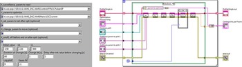
Components to be optimized are given as an array of settings and shared-variable paths to the optimizer class. Figure 2 shows an element of the array and the main program, which reads the settings and uses the class methods to optimize a beamline component. A LabVIEW program proceeds from left to right, with functions represented by square icons. The data between functions proceed along the wires between the functions. When each wire for a function has data ready (previous functions are done), that function is executed. Object-oriented LabVIEW adds simplicity to the code, with the whole object (class instance) with all its internal data proceeding in the same wire, and with only the class methods having permissions to change internal data. This reduces the often-encountered clutter of wires in larger LabVIEW projects and significantly improves the readability of the code. In addition, the inherent modularity of the different parts of a project results in easier modification and maintenance of the code. The optimization programs for each beamline component differ only by the input array. Optimization of the whole beamline is achieved simply by chaining the programs for the different beamline components in the order of the desired optimization.
The relevant parts of the LabVIEW program for beamline component optimization. Left: The input array for the optimizer. Right: The main LabVIEW code using the methods for scanning the parameter, fetching the profile data, plotting the results, and finding the maximum and committing the optimum value to the field.

The program package and the source code are available on request from the main author. The main requirement for the use of the program is a NI shared-variable interface to the accelerator together with an associated SQL database (e.g. NI Citadel).
PROFILES
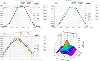
Figure 3 shows typical profiles for measured 14C count rate and 13C3+ current as a function of different parameters of the accelerator. Such graphical profiles have been instrumental in optimizing the system for high-precision AMS measurements.
Typical 1-D and 2-D profiles. Blue curves represent cubic spline fits and green curves Gaussian fits to the main measurand (shown in black). Different estimates for the maxima are given on the right of each figure. Vertical scales are arbitrary if different isotopes are shown. Upper left: 14C count rate (black) and 13C3+ current (red) as a function of the terminal voltage.

Because stable isotope currents are measured at a different point in the beamline than the rare-isotope events, the isotopes have a different acceptance as regards the preceding components. Hence, for some parameters, the beam profiles for the different isotopes may differ. Depending on the settings of other parameters in the system, the widths, shapes, or even the points of maxima can be different for the different isotopes. Fortunately, fast isotope pulsing (Palonen and Tikkanen Reference Palonen and Tikkanen2015) enables the optimizer to include all relevant isotopes in the same plot, enabling adequate detection and control over such cases. In addition, it is possible to optimize the beam using a suitably normalized sum of the isotopes.
The chosen goals of the optimization are as follows, in practical order of importance:
-
∙ Maximum current and/or count rate;
-
∙ Concurrent points of maxima for the different isotopes;
-
∙ Flat-top profile for each isotope; and
-
∙ Symmetric/non-skewed profile for each isotope.
Poor beam quality and less accurate AMS results are observed when these goals are not met, e.g. when a component is not at the setting of maximum beam current, the shape of a profile is highly skewed, or the point of maximum current or count rate is not the same for the different isotopes.
It is usually the case that when different isotopes do not have a concurrent maxima for a parameter, the settings of another component of the system are not optimal. In this case, practice has shown it to be best to optimize such component for the sum of all the isotopes, representing a suitable compromise over the isotopes, and optimize the component again after other components have been optimized. In this sense, the optimization is iterative.
In practice, the AMS system optimization is usually done by reading in from the database the settings of a similar AMS run and then running an optimization of roughly 20 essential parameters of the system.
CONCLUSIONS
The implemented routine for automatic optimization is fast, easy to use, robust to noise, and yields repeatable results. In addition, the graphical output in the form of beam current and count rate profiles is highly informative. Together with other improvements to the AMS system, along with optimal AMS data analysis (Palonen et al. Reference Palonen, Tikkanen and Keinonen2010), the automatic optimization has enabled us to push the precision of the system to better than 0.2%.