Implications
Real-time estimates of individual energy balance (EB) would enable early intervention in cases of excessive negative EB. The present method allows EB to be estimated solely from changes in BW measured automatically at milking (corrected for milk, foetus and gutfill) or from BW combined with body condition score (BCS) changes. Tested on 77 cows, the method was able to detect EB differences caused by small changes in concentrate amounts eaten. Standard body protein functions were developed, allowing EB to be estimated real-time for individual cows on farm without needing feed intake or BCS measurements. This EB method is a useful on-farm management tool.
Introduction
In high-producing dairy cows, lengthy periods of excessive negative energy balance (EB) have been linked to problems such as reduced reproductive performance (Oikonomou et al., Reference Oikonomou, Arsenos, Valergakis, Tsiaras, Zygoyiannis and Banos2008; Cutullic et al., Reference Cutullic, Delaby, Gallard and Disenhaus2012), digestive and locomotive disorders (Collard et al., Reference Collard, Boettcher, Dekkers, Petitclerc and Schaeffer2000), and metabolic diseases (Goff and Horst, Reference Goff and Horst1997). Therefore, the ability to assess the EB for individual cows in real-time and on farm would be a highly desirable management tool, enabling the dairy farmer to rapidly detect excessive negative EB. Traditional input–output methods to calculate EB require knowledge of individual feed intake (Hüttmann et al., Reference Hüttmann, Stamer, Junge, Thaller and Kalm2009), which is almost never available on commercial farms. In contrast, automated cow weighing technology, such as walk-over weights, is becoming increasingly common on commercial farms, where it is usually placed in the exit race of the milking parlour or the milking stall (in robotic milking systems). This type of technology offers the possibility of estimating individual EB on farm, because EB can be directly calculated from changes in mass of body reserves (Coffey et al., Reference Coffey, Emmans and Brotherstone2001). A method to estimate EB (EBbody) using daily BW measurements combined with frequent body condition score (BCS) measurements has recently been developed (Thorup et al., Reference Thorup, Edwards and Friggens2012). However, for commercial application, this method has two drawbacks. First, it requires reliable BCS measurements. Currently, these are difficult to obtain, because manual scoring is of limited precision, as are existing measuring technologies (i.e. ultrasound, image analysis). Consequently, the first aim of this study was to examine the extent to which the EBbody method can be simplified by basing EBbody on BW measurements alone, that is, removing the need for BCS measurements. Second, to allow early identification of cows with excessive negative EB, the method needs to work in real-time, which is currently not the case. A real-time method would also allow early detection of sudden changes in EB that would be indicative of individual cows going off-feed or of unplanned changes in ration quality. Thus, the second aim of this study was to adapt the EBbody method presented previously to become a real-time method. The third aim of the study was to evaluate the ability of a real-time EBbody model to detect short-term changes in EB.
Material and methods
Cows and experimental procedures
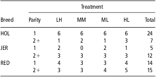
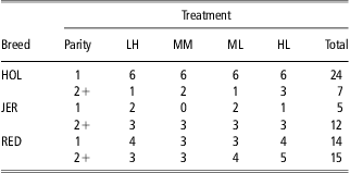
The data used to test the real-time EBbody method came from an already completed feeding experiment using 88 cows (Weisbjerg and Munksgaard, Reference Weisbjerg and Munksgaard2008). Therefore, it was not necessary to seek additional ethical committee approval to conduct the present study. This particular data set was well suited to test the ability of the method to detect short-term changes in EB, because the cows were given an increased concentrate allowance for a period during early or mid-lactation (see below). For the purpose of the present study, 11 cows were removed from data because of incomplete weight data over the lactation, leaving 77 cows in the present data set, calving from October 2005 to May 2006. All cows were loose-housed throughout the year in a barn at the Danish Cattle Research Centre (Tjele, Denmark) with an automatic milking system (Voluntary Milking System (VMS), DeLaval, Tumba, Sweden) and automatic feeding stations (Roughage Intake System, Insentec BV, Marknesse, The Netherlands). In the period from 0 to 195 days in milk (DIM) cows had ad libitum access to one of three TMRs that differed with respect to energy level (low: 0.84; medium: 0.88; high: 0.94 FU/kg DM), where one feed unit (FU) is equivalent to 7.89 MJ net energy (Weisbjerg and Hvelplund, Reference Weisbjerg and Hvelplund1993). In addition, cows were offered one of three different amounts of concentrate during milking, resulting in four main treatments: low TMR and high amount (4.4 kg/day) of concentrate (LH); medium TMR and medium amount (3.4 kg/day) of concentrate (MM); medium TMR and low amount (2.3 kg/day) of concentrate (ML); and high TMR and low amount (2.3 kg/day) of concentrate (HL). The VMS concentrate energy content was 0.95 FU/kg DM. From 75 to 105 DIM, half of the cows (spread equally across the four main treatments) had an increment of 0.2 kg/day concentrate intake (offered at milking). From 105 to 135 DIM, the other half of the cows had an increment of 0.5 kg/day concentrate intake. The experimental procedures and feed composition have been described in full by Weisbjerg and Munksgaard (Reference Weisbjerg and Munksgaard2008). For information, the distribution of cows between breeds, parities and main treatments is shown in Table 1, although these factors are not important for the real-time EBbody method evaluation in the present study.
The distribution of the 77 cows used to test the real-time EBbody method according to breed (HOL = Holstein; JER = Jersey; RED = Red), parity and main treatment (LH: low-energy TMR and high amount of concentratea; MM: medium-energy TMR and medium amount of concentratea; ML: medium TMR and low amount of concentratea; HL: high-energy TMR and low amount of concentratea)
aOffered at milking
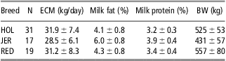
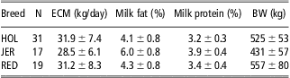
At each milking, cows were weighed automatically on a weighing platform (Bjerringbro Vægte, Bjerringbro, Denmark) installed in the VMS. Milk yield was registered at each milking and composite milk samples from all milkings in a 48-h period were taken and analysed for fat, protein and lactose content once a week. Energy corrected milk yield (ECM), milk fat percentage, milk protein percentage and smoothed BW averaged over the first 100 DIM for cows grouped by breed are in Table 2. BCS was assessed every 2 weeks by one of two trained observers to the nearest quarter unit on a scale from 1 (thin) to 5 (obese) (Ferguson et al., Reference Ferguson, Galligan and Thomsen1994).
Average daily ECM, milk fat percentage, milk protein percentage and BW ± s.d. during the first 100 DIM for 77 cows grouped by breed (HOL = Holstein; JER = Jersey; RED = Red)
Processing of cow BW data to allow calculation of EBbody
Adjusting BW for milk and meal-related gutfill
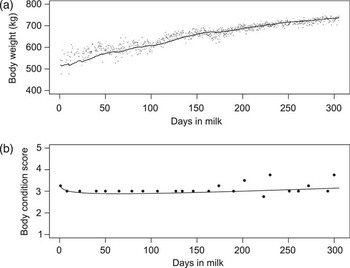
In the VMS, the cow stands on a weighing platform and the BW is recorded automatically during the entire milking. For each milking the end-weight, or so-called milk-free BW, was derived from the weighing platform data, described in detail by Thorup et al. (Reference Thorup, Edwards and Friggens2012). In brief, data were cleaned to exclude artefacts because of the cow being only partly on the weighing platform as it entered and left the milking stall, the remaining values were smoothed using a cubic spline with three knots. The smoothed value at the end of the milking is hereafter referred to as the milk-free BW. Each new observation of milk-free BW was compared with the mean of the previous two observations, and values differing by more than ±50 kg were disregarded. Over the whole data set this affected only 444 out of the 54 625 observations. The rest of the real-time BW smoothing procedure, to derive a meal-related gutfill-free BW, consisted of a double-exponential smoothing process in two steps: (1) single-exponential smoothing (SES) of data y 1, y 2,… with smoothing parameter w, where 0 < w < 1, was defined as St = St −1 + w(yt−St −1); (2) double-exponential smoothing (DES) was obtained by applying the SES scheme to the smoothed values St. If there was no trend in the data, then SES produces adequate smoothing of data and reliable forecastings. However, if there was a trend in the data, then DES must be used to obtain adequate smoothing and reliable forecastings. We used a modified DES procedure as follows: When the difference yt−St −1 was negative, the smoothing parameter was w = 0.08, and when yt−St− 1 was positive then w = 0.02. The result of this asymmetric weighting is that the smoothed curve follows a lower trajectory than if positive and negative differences were weighted equally. This downward bias is a means to minimize the influence of meal-related variation in gutfill on the smoothed BW, hereafter referred to as meal-related gutfill-free BW. The issue of accounting for meal-related association in gutfill is discussed in greater detail by Thorup et al. (Reference Thorup, Edwards and Friggens2012). An example of milk-free BW and the meal-related gutfill-free BW curve for one cow relative to DIM has been shown in Figure 1a.
Examples of (a) milk-free BW (kg) observations (points) and the smoothed, meal-related gutfill-free BW (line) relative to days in milk (DIM), and (b) body condition score (BCS, no unit) observations (circles) and smoothed BCS (line) of the same cow relative to DIM.

The lactations of the cows in the present study spanned a period from October 2005 to January 2007. Unfortunately, owing to loss of the raw weighing files from a database for a period of 4 months (February to May 2006), all lactations had a period of missing observations. However, BWs calculated as an average of the highest 100 weights during milking (Bossen et al., Reference Bossen, Weisbjerg, Munksgaard and Højsgaard2009) were available for all milkings, which allowed milk-free BW to be estimated for the missing periods by subtracting milk yield plus 9.2 kg from this ‘high’ BW. A total of 9.2 kg was the observed average difference between (high BW – milk yield) milk-free BW when both BW measures were available. This correction procedure worked well for the lactations of 77 cows; however, for 11 cows, transitions between estimated and observed data were uneven based on visual inspection, and therefore those 11 cows were excluded from this study.
Adjusting BW for conceptus weight
For the purpose of calculating EBbody, it is necessary to adjust BW for the weight gain associated with the conceptus, and therefore a conceptus-free BW is derived by subtracting the gravid uterus weight (W uterus, kg) from the meal-related gutfill-free BW. The W uterus is calculated as follows (Martin and Sauvant, Reference Martin and Sauvant2010a):
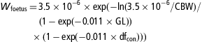 $$no{ {{W}_{{\rm{foetus}}}}\, {\rm{ = }}\,{\rm{3}}{\rm{.5}}\times {\rm{1}}{{{\rm{0}}}^{{\rm{ - 6}}}} \times {\rm{exp( - ln(3}}{\rm{.5}}\times {\rm{1}}{{{\rm{0}}}^{{\rm{ - 6}}}} {\rm{/CBW)/}} \cr \quad{{(1}}\,{\rm{ - }}\,{\rm{exp( - 0}}{\rm{.011}}\times {\rm{GL))}} \cr \,\times {\rm{(1}}\,{\rm{ - }}\,{\rm{exp( - 0}}{\rm{.011}}\times {\rm{d}}{{{\rm{f}}}_{{\rm{con}}}}{\rm{)))}} $$
 $${{W}_{{\rm{uterus}}}}\,{\rm{ = }}\,{\rm{(}}{{W}_{{\rm{foetus}}}}{\rm{/0}}{\rm{.58)/1000}}$$
where W foetus is weight of the foetus (g), GL is gestation length (days), CBW is future calf birth weight (g) and dfcon is days from conception (days). Gestation length is assumed to be 282 days, conception is assumed to be at 90 DIM and CBW is assumed to be 42 kg for Red cows, 44 kg for Holstein cows and 29 kg for Jersey cows. CBW numbers are herd means for the previous 5 years. There were no significant differences between parities in these values. In equation (2), the weight of the foetus is assumed to make up 58% of the gravid uterus weight.
Deriving empty body weight (EBW)
The difference between BW and EBW is assumed to be primarily because of the fill of the gut, udder and uterus. Udder fill is accounted for by the derivation of milk-free BW, uterine fill is accounted for by the derivation of conceptus-free BW and meal-related gutfill is accounted for by deriving meal-related gutfill-free BW. This leaves residual gutfill to be corrected for, which is done as follows:
 $${\rm{EBW}}\,{\rm{ = }}\,{\rm{conceptus}}\,{\rm{ - }}\,{\rm{free BW/(1}}\,{\rm{ + }}\,g\,\times \,({\rm{1}}\,{\rm{ - }}\,{\rm{\alpha }}\,{\rm{ - }}\,{\rm{\beta }}\,{\rm{\times }}\,{\rm{BCS)),}}$$
here the constant g is assumed to be 0.26 (kg/kg). The constants α and β are assumed to have the values 0.05 kg lipid/kg of EBW and 0.10 kg lipid/kg of EBW/unit of BCS, according to Friggens et al. (Reference Friggens, Ridder and Løvendahl2007b). Equation (3) assumes that the residual gutfill is a constant proportion of BW standardized to a constant body lipid content (Thorup et al., Reference Thorup, Edwards and Friggens2012). Thus, when comparing two cows of equal conceptus-free BW, but of differing BCS, residual gutfill will be less in the fatter cow transitioning into a higher EBW.
Smoothing BCSs
Given the inherent measurement errors associated with BCS, it is necessary to smooth these data. In the situation where BCS was measured with a high frequency (e.g. automated BCS measurement), this could be done using a real-time method similar to that used for the milk-free BW. However, in the present study high-frequency BCS data were not available, and therefore these data were instead smoothed using the following log-Woods model, called M1:
 $$no{{\rm{BCS}}\, {\rm{ = }}\,{{{\rm{(BCS1}}\,{\rm{\times }}\,{\rm{parity}}\,{\rm{\times }}\,{\rm{breed)}}}_{{\rm{lm}}}}\,{\rm{ + }}\,{{{\rm{(DIM}}\,{\rm{\times }}\,{\rm{parity}}\,{\rm{\times }}\,{\rm{breed)}}}_{{\rm{lm}}}} \cr \quad\,{\rm{ + }}\,{\rm{log(DIM)}}\,{\rm{\times }}\,{\rm{BCS1,}} \ \ \ \ \ \ \ \ \ \ \ \ \ \ \ \ \ \ \ \ \ \ \ \ \ \ \ \ \ \ \ \ \ \ \ \ \ (\rm M1)$$
where BCS1 is the observed BCS at one DIM, parity (l = 1, 2, 3+), breed (m = Holstein, Jersey, Red) and DIM (continuous). The notation of the three-way interactions implies that all main effects, pairwise interactions and the three-way interactions are included. An example of BCS observations and the smoothed BCS curve for one cow relative to DIM is shown in Figure 1b.
Calculating EBbody
Because any difference between energy inputs and outputs must be met by changes in body energy stores, EB (MJ/day) can be calculated from changes in body lipid and body protein as follows:
 $${\rm{E}}{{{\rm{B}}}_{{\rm{body}}}}\,{\rm{ = }}\,z\,{\rm{\times }}\,\rDelta {\rm{BL}}\,{\rm{ + }}\,y\,{\rm{\times }}\,{\rm{\rDelta BP,}}$$
where ΔBL is the rate of change in body lipid (kg/day); ΔBP is the rate of change in body protein (kg/day); z is the energy associated with ΔBL (MJ/kg); and y is the energy associated with ΔBP (MJ/kg). The values of the constants y and z differ for mobilization and deposition. Thus, y is 13.5 MJ/kg during mobilization of protein, that is, when ΔBP is negative, and 50.0 MJ/kg during deposition of protein, when ΔBP is positive. Similarly, z is 39.6 MJ/kg during mobilization, when ΔBL is negative, and 56.0 MJ/kg during deposition of lipid, when ΔBL is positive (Emmans, Reference Emmans1994).
ΔBL and ΔBP can be estimated from changes in EBW (ΔEBW, kg/day), changes in BCS (ΔBCS, units/day), and change in the product of EBW and BCS (Δ(EBW × BCS), kg units/day) using the following equations (details and assumptions are discussed by Thorup and colleagues (2012)):
 $$\rDelta {\rm{BL}}\,{\rm{ = }}\,{\rm{\alpha }}\,{\rm{\times }}\,\rDelta {\rm{EBW}}\,{\rm{ + }}\,{\rm{\beta }}\,{\rm{\times }}\,\rDelta {\rm{(EBW}}\,{\rm{\times }}\,{\rm{BCS)}}$$
and
 $$\rDelta {\rm{BP}}\,{\rm{ = }}\,k{\rm{(}}\rDelta {\rm{EBW}}\,{\rm{ - }}\,\rDelta {\rm{BL)}}$$
here k (= 0.2224 kg/kg) is a constant giving the protein content of lipid-free EBW. The constants k, y and z can be regarded as generic, and the energy units used are effective energy (EE) described by (Emmans, Reference Emmans1994). In this system, 1 MJ of EE supply has the same energy value as 1 MJ of lipid loss from the body.
Finally, the EBbody observations were smoothed after first disregarding observations differing more than ±30 MJ EE/day from the mean of the previous two observations (3998 out of 54 625 observations). The remaining observations were real-time smoothed (double-exponentially and symmetrically, that is, using the same smoothing parameter (w = 0.03) for both positive and negative differences).
Estimating ΔBPstd
Having BCS measurements in addition to BW allows direct estimation of lipid content and thereby ΔBL. Given this, ΔEBW can easily be separated into ΔBL and ΔBP. However, if one wishes to calculate EBbody without using BCS data, then another means to estimate the relative contributions of ΔBL and ΔBP to ΔEBW is needed, because there is no a priori reason to assume that BL : BP remains constant through time. Given that ΔBP is relatively small for most of lactation (Gibb and Ivings, Reference Gibb and Ivings1993), it may be reasonable to assume a standard function for ΔBP relative to DIM, hereafter called ΔBPstd. This permits ΔBL to be estimated from ΔEBW as follows:
 $$\rDelta {\rm{Lipid - free}}\,{\rm{EB}}{{{\rm{W}}}_{{\rm{std}}}}\,{\rm{ = }}\,\rDelta {\rm{B}}{{{\rm{P}}}_{{\rm{std/}}k}}$$
 $$\rDelta {\rm{BL}}\,{\rm{ = }}\,\rDelta {\rm{EBW}}\,{\rm{ - }}\,\rDelta {\rm{B}}{{{\rm{P}}}_{{\rm{std/}}k}}$$
It then remains to estimate ΔBPstd. Data on directly measured ΔBP are scarce and usually come from serial slaughter experiments with limited number of animals. In the present study, we chose to examine the feasibility of using equations (5) and (6) in the present paper to provide the standard curves through lactation. To avoid bias in estimation of ΔBPstd curves, we first excluded the sensitivity of equation (5) to the chosen values of coefficients α and β, the regression coefficients for converting BCS to body lipid content. This was done by comparing the cumulative EBbody (using different values of α and β) with the EBW change from the point where EBbody becomes positive until 240 DIM:
 $$no{\rDelta {\rm{B}}{{{\rm{W}}}_{{\rm{estimated}}}}\,{\rm{(kg)}}\,{\rm{ = }}\,{\rm{(cumulated}}\,{\rm{E}}{{{\rm{B}}}_{{\rm{body}}}}\,{\rm{(MJ)/}}\cr \quad{{56}}\,{\rm{(MJ/kg))/0}}{\rm{.77}}{\rm{.}} $$
Here 56 MJ/kg is the amount of energy required to create 1 kg lipid (see equation 4) and 0.77 is the lipid proportion of live weight gain (Wright and Russel, Reference Wright and Russel1984). Cows of third parity and older were used for this comparison, on the assumption that these animals were mature, and therefore there was no overall change in body protein. Two of the 13 mature cows experienced a weight drop starting shortly after 200 DIM, and consequently the period for these two cows was cut-off at 200 DIM to ensure that all cows gained BW during the period investigated.
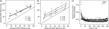
First, the ΔBW estimated from cumulated EBbody was compared with the observed ΔEBW for three different combinations of α (0.04; 0.05; 0.06) at a fixed value of β (0.10) as shown in Figure 2a. Varying coefficient α only had minor effects on intercept and slope. As α increased from 0.04 to 0.06, the slope increased from 0.80 to 0.82 (±0.10 kg/kg) and the intercept increased from 42.3 to 43.6 (±7.0 kg). In all cases, the R 2 was 0.84 and the slope was not significantly different from unity.
Estimated EBW change (kg) calculated from cumulative EBbody plotted against measured EBW change (kg) for the 13 mature cows: (a) values of α = 0.04; 0.05; 0.06 with β = 0.10; (b) values of β = 0.08; 0.10; 0.12 with α = 0.05. A line of unity is included to ease comparison of slopes. The period of change was from the time of EBbody becoming positive until 240 days in milk (DIM); and (c) difference (mean and s.d.) between ΔBPstd calculated with β = 0.12 and b = 0.10 (kg/day) relative to DIM, n = 77.

In a second step, ΔBW estimated from cumulated EBbody was compared with the observed ΔEBW with coefficient α kept constant (0.05) and three values of β (0.08; 0.10; 0.12) as shown in Figure 2b. Varying coefficient β had major effects on the slope and intercept. Increasing β from 0.08 to 0.12 increased the slope from 0.72 to 0.91 (±0.13 kg/kg; R 2 = 0.81), this latter slope was significantly different from unity. Over the same range in β, the intercept increased from 35.0 to 51.4 (±8.9 kg). The combination of α = 0.05 and β = 0.12 resulted in a slope close to unity, and because 0.12 is closer to prior estimates in the literature than 0.10 (Wright and Russel, Reference Wright and Russel1984), it was decided to adjust β accordingly. All data presented hereafter are calculated on the basis of this combination of α and β.
To estimate the influence of β on ΔBPstd, the difference between ΔBPstd calculated with β = 0.12 and ΔBPstd calculated with β = 0.10 for all cows is shown in Figure 2c. The figure indicates that changing the value of coefficient β has very little effect on the ΔBPstd curve.
Deriving a ΔBPstd function
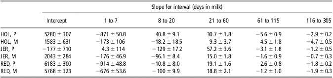
Having adjusted coefficient β to 0.12, ΔBPstd was calculated using equations (5) and (6) for the different breeds and parities. Finally, continuous piecewise linear regression was used to establish ΔBPstd as a function of DIM for each combination of breed and parity separately. In previous research on body reserve changes over lactation, breakpoints at days 7, 20, 60 and 115 have been used successfully (Friggens et al., Reference Friggens, Berg, Theilgaard, Korsgaard, Ingvartsen, Løvendahl and Jensen2007a), and therefore knots were placed at these breakpoints (and at the endpoints).
Statistical analysis
All processing of data and statistical analysis was performed in R (R Development Core Team, 2011).
The testing of the real-time method of calculating EBbody to detect short-term changes in EB was carried out using data from two periods: 70 to 90 DIM and 130 to 145 DIM. In the first period, half of the cows experienced an increase in concentrate intake starting on day 75. In the second period, half of the cows experienced a decrease in concentrate intake starting on day 135. In both periods, average EBbody was calculated for 5-day intervals starting 5 days before the change in concentrate intake (at 75 and 135 DIM for increased and decreased concentrate intake, respectively). Before–after EBbody differences were then calculated by subtracting the before 5-day average from either the 0 to 5, 5 to 10 or 10 to 15 days after change average, yielding three EBbody differences (MJ EE/day): ΔEB5, ΔEB10 and ΔEB15 for the 70 to 90 DIM period containing the concentrate decrease and two EBbody differences (MJ EE/day): ΔEB5, and ΔEB10 for the 130 to 145 DIM period containing the concentrate decrease.
For each period separately, the effects of breed, parity, main treatment and concentrate change on the EBbody differences were tested in a linear model (M2) using the lme4 package in R:
 $$no{{{Y}_{ijkl}}\, {\rm{ = }}\,{\rm{\mu }}\,{\rm{ + }}\,bree{{d}_i}\,{\rm{ + }}\,parit{{y}_j}\,{\rm{ + }}\,treatmen{{t}_k}\,\cr \quad{\rm{ + }}\,chang{{e}_l}\,{\rm{ + }}\,{\epsilon}ij{{k}_l}{\rm{,}} \rm(M2)$$
where the response variable Y was the difference in EBbody of the ijklth observation, μ was the overall mean, the explanatory effects were: breed (i = Holstein, Jersey, Red), parity (j = 1, 2+), main treatment (k = LH, ML, MM, HL), change (l = changed, unchanged (to distinguish the cows for which concentrate intake was changed from those not changed)). εijkl was the residual error term associated with the ijklth observation. Further, the six possible two-way interactions were included in the initial model. The insignificant interactions were removed stepwise for each response variable. Owing to low numbers of cows (see Table 1) three-way interactions were not tested.
Results
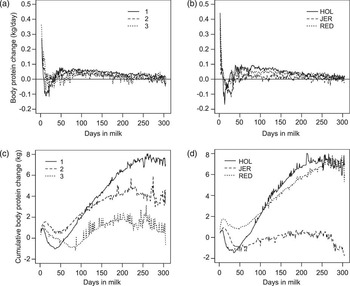
The estimated ΔBPstd across lactation is shown by parity (Figure 3a) and breed (Figure 3b). These curves have not been smoothed; nevertheless, they show that the largest daily BP changes take place during early lactation (before 40 DIM). With a few exceptions, the curves stay between −0.1 and 0.1 kg/day after 6 DIM, and thus BP changes account for energetic changes between 1.4 and 5.0 MJ EE/day from 1 week after parturition and onwards through lactation. The spike in ΔBP immediately post partum is most likely an artefact related to peri partum liveweight disturbances. Further, as expected, primiparous cows seemed to have larger BP changes, followed by second parity and third parity cows. By visual inspection, Holstein cows seemed to exhibit larger BP changes, and Jersey cows seem to exhibit the lowest BP changes of the breeds studied; however, for the Holstein cows, the large BP changes may be reflecting the fact that there was a greater proportion of heifers in this breed sample.
Average estimated ΔBPstd (kg/day) relative to days in milk (DIM) grouped by (a) parity and (b) breed: HOL = Holstein; JER = Jersey; RED = Red. Average cumulative ΔBPstd (kg) relative to DIM by (c) parity and (d) breed, n = 77.

The cumulative ΔBPstd across lactation is shown by parity in Figure 3c and by breed in Figure 3d. Not surprisingly, immature cows, not only of first lactation but also of second lactation, show a net gain of BP through lactation, whereas the mature cows of third lactation and older do not have a net gain of BP (Figure 3c). Holstein and Red cows show a net gain of BP through lactation, whereas Jersey cows do not seem to gain BP over lactation (Figure 3d).
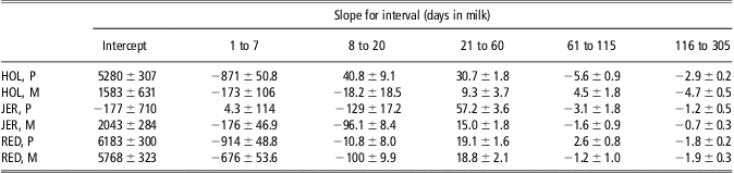
The regression coefficients of the piecewise linear regression of ΔBPstd by breed and parity has been shown in Table 3 and Supplementary Figure S1.
Regression coefficients for ΔBPstd (kg/day) ± s.d. × 10−4 for each combination of breed (HOL = Holstein; JER = Jersey; RED = Red) and parity (P = primiparous; M = multiparous), n = 77
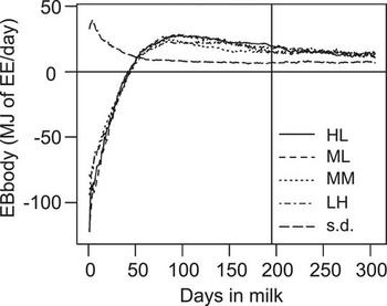
The average EBbody trajectories and mean s.d. relative to DIM for cows grouped by main treatment has been shown in Figure 4. The four main treatments followed the same EBbody trajectory, with HL treatment almost consistently exhibiting the highest EBbody throughout the experimental period, although, as can be deduced from the s.d., which is also presented relative to DIM, this difference was not significant at any time in lactation. This is in agreement with the EB results calculated from intake and milk production (Weisbjerg and Munksgaard, Reference Weisbjerg and Munksgaard2008). Figure 4 also shows that the s.d. is greatest during early lactation.
Average energy balance (EBbody; MJ of EE/day) and mean s.d. relative to days in milk grouped by main treatment, n = 77. The vertical line marks the end of the experimental period.

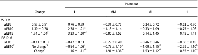
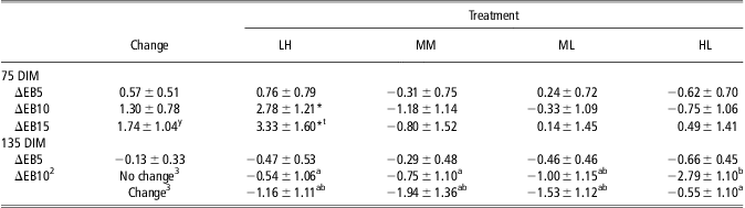
The ability of the EBbody method to detect small changes in EB was tested by comparing differences between EBbody (MJ/day) before and after a change in concentrate intake (an increase of 0.2 kg/day at 75 DIM and a decrease of 0.5 kg/day at 135 DIM), relative to the equivalent difference for cows that did not change concentrate intake. For simplicity only the effects of treatment and concentrate change are shown in Table 4, the effects of parity and breed are reported in the text when significant. The EBbody differences were calculated as level after change minus level before change, and thus positive differences denote that EBbody increased after the change. Across main treatments, the average effect of the increase in concentrate intake of 0.2 kg/day on EBbody was estimated as 0.57, 1.30 and 1.74 MJ/day in the first, second and third 5-day periods after the change. The difference in the third 5-day period (ΔEB15) had a P value < 0.1. There was no significant interaction between this effect (of concentrate intake change) and the main feeding treatment, although there were minor differences between breeds with Red cows increasing EBbody significantly more than Holstein cows (contrast = 1.67 ± 0.60 MJ/day for ΔEB5).
Differences in EBbody (MJ/day) over a 5-, 10- or 15-day period at either 75 DIM or 135 DIM.
DIM = days in milk.
*Contrast significantly different from zero. t,yP < 0.1. a,bP < 0.05.
1See Table 1 for explanation of treatment abbreviations.
2M2 plus treatment × change interaction.
3For EB10 when concentrate intake was decreased, there was a significant treatment × change interaction; consequently, the main treatment effects are shown separately for cows that did or did not change concentrate intake.
Baseline differences are shown for cows that did not change concentrate intake for each of the four underlying feeding treatments (LH, ML, MM and HL)1) together with the additional effect of a change in concentrate intake (column ‘change’). At 75 DIM, the change in concentrate intake (for those cows that changed) was an increase of 0.2 kg, and there was no significant interaction between change and feeding treatment. At 135 DIM, concentrate intake (for those cows that changed) was decreased by 0.5 kg, and there was a significant interaction between change and feeding treatment, shown in the last row of the table. EBbody differences are calculated between average values before; and 5 days after change (ΔEB5), 10 days after change (ΔEB10) and 15 days after change (ΔEB15). The effects of treatment and concentrate change are reported as contrasts ± s.e., that is, they should be added to the reference level, which is for LH cows that did not change, to give the absolute size of the effect. The increase in concentrate intake started incrementally at 75 DIM, the decrease was immediate at 135 DIM.
When concentrate intake was decreased by 0.5 kg/day, there was a significant difference in EBbody change 10 days after the change relative to cows that did not change intake, on three out of the four main feeding treatments (significant treatment × concentrate intake change interaction; Table 4).
Discussion
This paper has presented a tool that estimates individual EBbody in real-time from frequent BW measurements, either in combination with BCS measurements or alone. For use in the latter case, we have provided proof of principle that ΔBPstd curves as a function of DIM can be developed for the breeds and parities investigated. These ΔBPstd are close to zero for most of the lactation. The real-time functionality that has been added is an important feature for the deployment of the method as an on-farm management diagnostic. In this context, it has been shown that the EBbody tool is capable of detecting EBbody changes caused by relatively small concentrate intake changes (0.2 kg/day).
The present study intended to develop a real-time indicator of EBbody with the potential to be deployed on-farm, which was achieved by applying a real-time smoothing method to the frequent BW data. The BCS data were smoothed using a log-Woods procedure, which can be used until fully automated BCS technology becomes available, or BCS can be smoothed real-time with recursive least squares. Moreover, an alternative option was provided by the ΔBPstd function, where no BCS is needed, with relatively little loss of precision.
EBbody has previously been shown to compare well with the traditional EB calculated as energy input minus output (Thorup et al., Reference Thorup, Edwards and Friggens2012), and therefore the main issue of the present study was to investigate whether small changes in EB (caused by small changes in concentrate intake) could be detected by this method. The results showed that the new real-time functionality allowed differences in EBbody changes caused by a concentrate increase to be detected already within 5 days after the increase, as Red cows increased EBbody significantly more than Holstein cows. In addition, from 10 days post-change, the cows having an increase in concentrate intake increased their EBbody significantly more than cows not receiving an increase in concentrate intake.
Further, in this study, the generality of the tool presented previously (Thorup et al., Reference Thorup, Edwards and Friggens2012) was extended, because pregnancy effects are now adjusted for by subtracting the estimated weight of conceptus from BW before EBbody calculation. This correction procedure means (assuming that conception is at 90 DIM) for the Holstein cows, which give birth to the heaviest calves (44 kg) of the three breeds investigated, that the gravid uterus weighs 23 kg at 305 DIM and 75 kg at calving. For this study, conception was assumed to be at 90 DIM; however, the EBbody estimates would be more precise if, for example, individual dates of insemination were used, and therefore in an on-farm situation we would recommend using the latter. As the method is now, it becomes simpler to use the real-time information about the sign of ΔBL and ΔBP (positive or negative) to assign the appropriate energy constants (y and z), which differ for mobilization and deposition of BL and BP in the calculation of EBbody. Thus, individualized transition points between mobilization and deposition are used in the real-time method. The benefit of using individualized transition points is that transitions become smooth instead of disrupted for some individuals when fixed transition points are used (Thorup et al., Reference Thorup, Edwards and Friggens2012).
The tool presented in this study does have limitations, because it requires an estimate of gutfill. This was partly handled by calculating a milk, conceptus and meal-related gutfill-free BW, thus leaving only the residual gutfill to be estimated. The residual gutfill was assumed constant over time in accordance with Martin and Sauvant (Reference Martin and Sauvant2010b), being affected only by animal size, because differences in feed composition and differences owing to prior feed intake both tend towards zero with time. It would be desirable to validate the EBbody presented here on larger, independent data sets to confirm the robustness of the method, specifically in relation to different diet types. Here, differences in forages and especially grazing v. indoor feeding will be important tests. It will also be important to validate the BPstd curves proposed in this study on a larger population.
Finally, the present study estimates EBbody for lactating cows, because the weights are measured in connection with milking; however, if dry cows were weighed on a daily basis, EBbody could be equally well calculated for the dry period. That would give the farmer an estimate of the cow's EBbody during the transition period, a crucial part of the cow's life. But currently, frequent BW measurements on dry cows are not available to us.
Conclusions
A real-time method for deriving EB from frequent BW measures either alone or in conjunction with BCS measures has been developed. This extends the applicability of the method as real-time measures can be used for decision support and early intervention. The real-time method was shown to be able to detect relatively small changes in dietary energy supply. In addition, adjustments for pregnancy weight change and flexible transition between tissue mobilization and accretion phases have been included. This method can be an important practical management tool with the huge advantage of not needing data on feed intake or feed composition, or BCS.
Future work should focus on validating the present EBbody method on independent data sets to confirm the robustness of the method.
Acknowledgements
This work was part of the ‘In-line monitoring technology, biomarkers, sensor technology, risk management and expert systems’ project funded by the Danish National Advanced Technology Foundation. The funding body had no involvement with this study. We thank the staff at DCRC for performing the BCS and Connie Middelhede, Department of Animal Science, Aarhus University, for help in making the raw weight data accessible.