1. INTRODUCTION
By definition, two simultaneously operating GPS receivers with distance apart greater than many hundreds of kilometres form a long-baseline (Blewitt, Reference Blewitt1989). Basically, the deployments of the two receivers are possibly different: one of them (pivot receiver) needs to be placed at a location with precisely known position, while the other (rover receiver) is allowed to occupy locations whose positions can be either known or unknown (Eckl et al., Reference Eckl, Snay, Soler, Cline and Mader2001). Up to now, the long-baseline setup has been adopted across a broad range of applications such as relative positioning (Eckl et al., Reference Eckl, Snay, Soler, Cline and Mader2001; Schüler, Reference Schüler2006), time transfer (Lee et al., Reference Lee, Schutz, Lee and Yang2008; Petit and Jiang, Reference Petit and Jiang2008) and atmosphere sensing (Jin et al., Reference Jin, Luo and Ren2010; Pacione and Vespe, Reference Pacione and Vespe2003). To maximise the efficiency and accuracy of these applications, fast and successful Integer Ambiguity Resolution (IAR) is always essential, so that the very precise Double-Differenced (DD) carrier-phase data can be fully exploited (Blewitt, Reference Blewitt1989; Bock et al., Reference Bock, Abbot, Counselman, Gourevitch and King1985; Li and Teunissen, Reference Li and Teunissen2011). Unfortunately, GPS long-baseline IAR is not a trivial task, since it has to tackle the non-negligible atmospheric delays underlying the DD data (Jin et al., Reference Jin, Luo and Ren2010; Schüler, Reference Schüler2006; Teunissen, Reference Teunissen1998a).
Already employed by the Bernese GPS software, the Quasi Ionosphere-Free (QIF) and the Wide-lane/Narrow-lane (WN) are two sophisticated strategies particularly suitable for GPS long-baseline IAR (Dach et al., Reference Dach, Hugentobler, Fridez and Meindl2007). In principle, QIF estimates dual-frequency float ambiguities from DD data and then resolves them by means of searching (Mervart et al., Reference Mervart, Beutler, Rothacher and Wild1994). The search range defined for each float ambiguity depends solely on its empirical precision. To optimise searching efficiency, it would be wise to incorporate ionospheric constraints so as to obtain the float ambiguities to high precision. The WN is however a two-step strategy resolving first the wide-lane ambiguities (by the integer rounding method) and then the narrow-lane ones (by the integer bootstrapping method) (Teunissen, Reference Teunissen1998b). The WN employs the Melbourne-Wübbena (MW) and the ionosphere-free linear combinations, respectively, in order to circumvent the effects of ionosphere on wide-lane and narrow-lane IAR (Blewitt, Reference Blewitt1989).
Still, a number of typical pitfalls behind the QIF or the WN are identifiable. Introducing ionospheric constraints to the QIF implies that a choice between deterministic (single-layer) and stochastic modelling of the ionosphere needs to be made. However, the ionosphere reproduced by the single-layer model is subject to the combined levelling and model error effects, the overall size of which may reach a few tens of decimetres (Brunini and Azpilicueta, Reference Brunini and Azpilicueta2009); likewise, in many cases, the stochastic ionosphere modelling does not work well either, mainly due to a lack of good a priori ionospheric corrections (Odijk, Reference Odijk2001; Teunissen, Reference Teunissen1998a). As a crucial prerequisite for WN, resolving wide-lane ambiguities using the MW linear combination does not have to take special care of the ionosphere contributions, but its reliability depends largely on the quality of the code data (Dach et al., Reference Dach, Hugentobler, Fridez and Meindl2007).
Moreover, both the QIF and the WN estimate the between-receiver relative Zenith Tropospheric Delays (ZTDs), among others, to cope with the tropospheric delays (Jin et al., Reference Jin, Luo and Ren2010). GPS satellites observed at low elevation angles are quite helpful for relative ZTD estimation (Douša, Reference Douša2010), but they are unlikely to be in the common view of both receivers and thus are discarded when formulating the DD data (Bar-Sever et al., Reference Bar-Sever, Kroger and Borjesson1998; Petit and Jiang, Reference Petit and Jiang2008). This has a consequence that successful IAR with either the QIF or the WN begins to be possible only after processing quite long periods of GPS data (typically 8–24 hours) (Dach et al., Reference Dach, Hugentobler, Fridez and Meindl2007). As the time required for IAR increases, the benefits brought by the IAR to some applications would be gradually lowered (Teunissen, Reference Teunissen1995).
In this contribution, we attempt to solve the bottleneck problems of GPS long-baseline IAR stemming from the atmospheric delays. The precise Point Positioning (PPP) method using zero-differenced (ZD) GPS data is able to make good use of more information than DD data processing (Kouba, Reference Kouba2009; Zumberge et al., Reference Zumberge, Heflin, Jefferson, Watkins and Webb1997), typically the GPS data of non-common view satellites, and the precise satellite clocks routinely delivered by International Global Navigation Satellite System service (IGS) along with the orbits (Dow et al., Reference Dow, Neilan and Rizos2009). So far PPP has been proven capable of providing centimetre-level ZTDs and decimetre-level Slant Ionospheric Delays (SIDs) (Leandro et al., Reference Leandro, Santos and Langley2011; Zhang et al., Reference Zhang, Ou, Yuan and Li2012). With these general facts in mind, we develop the idea of using PPP to estimate the ZTDs and the SIDs for both the pivot receiver and the rover receiver, respectively. After that, we reformulate these PPP-derived atmospheric delays into uncertain constraints that can be easily incorporated into the QIF-based IAR process.
We remark that some applications that traditionally rely on the long-baseline set up can nowadays be served also by the IAR-enabled PPP technique (a.k.a. PPPAR) (Ge et al., Reference Ge, Gendt, Rothacher, Shi and Liu2008, Laurichesse et al., Reference Laurichesse, Mercier, Berthias, Broca and Cerri2009). However, the applicability of PPPAR would be limited by the availability of externally provided information on GPS satellite carrier-phase biases. At the same time, most PPPAR implementations still follow the WN strategy for IAR, thus implying that it would still need a few hours for the PPPAR to achieve favourable IAR performances (Geng et al., Reference Geng, Meng, Dodson, Ge and Teferle2010, Laurichesse et al., Reference Laurichesse, Mercier, Berthias, Broca and Cerri2009). To speed up the IAR in the context of PPPAR, investigations into the possibility of incorporating external atmospheric corrections are still ongoing (Banville et al., Reference Banville, Collins, Zhang and Langley2014, Geng et al., Reference Geng, Teferle, Meng and Dodson2011). For these reasons our study on the GPS long-baseline IAR is still of relevance.
The remainder of this contribution is organised as follows. In Section 2, we revisit briefly the ZD and DD variants of dual-frequency GPS observation equations after linearization. The ZD variant forms the basis for our derivations of the PPP model in Section 3, while the DD variant is used to illustrate the fundamental procedures of our proposed QIF in Section 4. We report in Section 5 the results of numerical tests dedicatedly designed to verify the empirical precision of PPP-derived ZTDs/SIDs, and to compare the performance between our proposed QIF and the standard WN. We conclude in Section 6.
2. GPS OBSERVATION EQUATIONS
As our point of departure, we briefly revisit the ZD and DD variants of linearized observation equations for dual-frequency GPS code and carrier-phase data, respectively.
2.1. ZD variant
Let us assume that two receivers q (pivot) and u (rover) are able to track dual-frequency GPS data from m and n satellites, respectively. As we consider only the long-baseline setup in this contribution, the m is not necessarily equal to n. Given certain receiver-satellite channel r − s, the ZD variant of linearized observation equations reads (Leick, Reference Leick2004),
 $$\eqalign{& E\{ p_{r,j}^s \} = - \left[ {{\bf u}_r^{s}} \right]^T{\bf x}_r + g_r^{s} \tau _r + dt_r - dt^{s} + \mu _j\iota _r^{s} + b_{r,j} - b_{,j}^{s} \cr & E\{ \phi _{r,j}^{s} \} = - \left[ {{\bf u}_r^{s}} \right]^T{\bf x}_r + g_r^{s} \tau _r + dt_r - dt^{s} + \mu _j\iota _r^{s} + \lambda _{\,j}z_{r,j}^{s}} $$
where E{ · } denotes the expectation operator, s = 1…m (s = 1…n) for receiver r = q (r = u), frequency index j = 1,2. ZD code and carrier-phase data (both in distance units) for each frequency are denoted as
 $p_{r,j}^s $
and
 $\phi _{r,j}^s $
, to which the approximate geometric ranges computed from approximate receiver position
 ${\bf x}_r^0 $
and precisely known satellite positions
 ${\bf x}^s$
have already been applied. The rest of our notations are interpreted as follows.
 ${\bf x}_r$
the incremental receiver position with respect to
 ${\bf x}_r^0 $
,
 ${\bf u}_r^s $
the receiver-satellite unit vector, τ
r
the ZTD with mapping function denoted as
 $g_r^s $
, dt
r
(dt
s
) the receiver (satellite) clock,
 $z_{r,j}^s $
the dual-frequency non-integer ambiguities absorbing receiver and satellite phase delays (in cycles) with wavelengths denoted as λ
j
,
 $\iota _r^s $
the SID with coefficient denoted as
 $\mu _j = \lambda _j^2 /\lambda _1^2 $
and b
r,j
(
 $b_{,j}^s $
) the receiver (satellite) code delays for each frequency.
When we are about to formulate the PPP model by incorporating the ZD observation equations like Equation (1) for multi-epoch, multi-satellite data collected by a stand-alone GPS receiver, special care should be taken of the following issues. First, a variety of correction terms such as satellite clock offsets, satellite attitude effects and site displacements must be applied (Héroux and Kouba, Reference Héroux and Kouba2001; Kouba, Reference Kouba2009). Second, the behaviours of unknowns as a function of time have to be reasonably characterised: ambiguities will remain constant as long as no cycle slips occur; ZTDs as well as the SIDs are estimated as a random walk process; receiver clocks are treated as epoch-wise unknowns. Third, with respect to the pivot receiver (r = q), since its position is already a priori known, it makes more sense to exclude the incremental receiver position (
 ${\bf x}_q$
) from the unknown vector.
2.2. DD variant
Considering a pair of GPS satellites t and s that are in common view of receivers q (pivot) and u (rover), simply double-differencing their linearized ZD observation equations will yield the following DD counterparts,
 $$\eqalign{& E\{ p_{qu,j}^{ts} \} = - \left[ {{\bf u}_u^{ts}} \right]^T{\bf x}_u + g_u^{ts} \tau _{qu} + \mu _j\iota _{qu}^{ts} \cr & E\{ \phi _{qu,j}^{ts} \} = - \left[ {{\bf u}_u^{ts}} \right]^T{\bf x}_u + g_u^{ts} \tau _{qu} - \mu _j\iota _{qu}^{ts} + \lambda _jz_{qu,j}^{ts}} $$
where ( · )
qu
= ( · )
u
− ( · )
q
denotes a variable between receivers u and q; likewise ( · )
ts
= ( · )
s
− ( · )
t
denotes a variable between satellites s and t (used as the pivot satellite);
 $\left( \cdot \right)_{qu}^{ts} = \left( \cdot \right)_u^{ts} - \left( \cdot \right)_q^{ts} $
denotes a DD observable or variable. Note that in contrast to what is expressed by Equation (1), the (receiver and satellite) clocks and code delays have already been eliminated, leaving a set of estimable unknowns:
 ${\bf x}_u$
the incremental receiver position, τ
qu
the relative ZTD,
 $\iota _{qu}^{ts} $
the DD SID,
 $z_{qu,j}^{ts} $
the DD integer ambiguities.
Notably, one tacit assumption has been made by us when setting up Equation (2). That is for a given GPS satellite (s for example),
 $g_q^s \approx g_u^s $
. As far as the GPS long-baseline set up is concerned, such assumption holds only for GPS satellites observed at rather high elevation angles (≥ 20°). Were the DD data from GPS satellites with lower elevation angles (5–15°) be included further, it becomes indispensable to introduce the tropospheric gradients to Equation (2) as additional unknowns. Actually, precise estimation of tropospheric gradients might require daily DD data (Bar-Sever et al., Reference Bar-Sever, Kroger and Borjesson1998). This seems to be unfavourable for our study, in view of the fact that the sole goal of this contribution is to achieve fast and successful GPS long-baseline IAR.
Although the satellite clock offsets are made available by IGS together with the precise orbits, in contrast to PPP, they are not necessary for DD data processing. In addition, to construct the DD data, the satellites that can only be observed by one receiver (either the pivot or the rover) are not usable any more.
3. ATMOSPHERIC DELAY DETERMINATION WITH PPP
In general, the customary PPP model treats the SIDs as nuisance unknowns and removes them by forming ZD ionosphere-free code and carrier-phase data (Zumberge et al., Reference Zumberge, Heflin, Jefferson, Watkins and Webb1997). In this section, we develop a different PPP model directly employing ZD data to enable the simultaneous estimation of ZTDs and SIDs. For simplicity's sake, we restrict the derivation of PPP model only to the pivot receiver (r = q). One can readily duplicate our derivations for the rover receiver (r = u) as well. The only difference is whether or not the receiver position is assumed to be precisely known.
ZD observation equations represented by Equation (1) for the pivot receiver are unlikely to be solvable, because the unknowns involved cannot be separated from one another. We undertake the following two steps to overcome this problem.
In the first step, we re-parameterise, respectively, the dual-frequency code delays for the pivot receiver (b
q,j
) and the satellite (
 $b_{,j}^s $
) as follows
 $$\left\{ {\matrix{ {b_{q,j} = b_{q,IF} - \mu _jb_{q,GF}} \cr {b_{,j}^s = b_{,IF}^s - \mu _jb_{,GF}^s} \cr}} \right.$$
for j = 1,2 and s = 1…m; where
 $b_{q,IF} = \displaystyle{1 \over {\mu _2 - 1}}\left( {\mu _2b_{q,1} - b_{q,2}} \right)$
and
 $b_{q,GF} = \displaystyle{1 \over {\mu _2 - 1}}\left( {b_{q,1} - b_{q,2}} \right)$
denote the ionosphere-free and the geometry-free linear combinations of b
q,j
, respectively; likewise,
 $b_{,IF}^s $
and
 $b_{,GF}^s $
denote two linear combinations of
 $b_{,j}^s $
. Note that, b
q,GF
(
 $b_{,GF}^s $
) is also known as scaled receiver (satellite) Differential Code Bias (DCB) (Brunini and Azpilicueta, Reference Brunini and Azpilicueta2009; Ciraolo et al., Reference Ciraolo, Azpilicueta, Brunini, Meza and Radicella2007; Jin et al., Reference Jin, Jin and Feng2012).
The re-parameterised (receiver and satellite) code delays given in Equation (3) are inestimable and thus should be lumped with other unknowns than the ZTD τ r . While doing so, the reformulated ZD code observation equations read
 $$E\{ p_{q,j}^s \} = g_q^s \tau _r + d\,\bar t_q - d\,\bar t^s + \mu _j\bar \iota _q^s $$
where
 $d\,\bar t_q - dt_q + b_{q,IF}$
(
 $d\,\bar t^s - dt^s + b_{,IF}^s $
) is the redefined receiver (satellite) clock and
 $\bar \iota _q^s = \iota _q^s + b_{,GF}^s - b_{q,GF}$
is the redefined SID.
Introducing those redefined unknowns given in Equation (4) to the ZD carrier-phase observation equations, we then get
 $$E\{ \phi _{q,j}^s \} = g_q^s \tau _r + d\,\bar t_q - d\,\bar t^s - \mu _j\bar \iota _q^s + \lambda _j\bar z_{q,j}^s $$
where
 $\bar z_{q,j}^s = z_{q,j}^s - \displaystyle{1 \over {\lambda _j}}\left[ {\left( {b_{q,IF} - b_{,IF}^s} \right) - \mu _j\left( {b_{,GF}^s - b_{q,GF}} \right)} \right]$
are the redefined ambiguities.
The next step is to take advantage of the IGS precise satellite clocks, so as to eventually yield the following PPP model of our interest
 $$\eqalign{& E\{ p_{q,j}^s + d\,{\tilde t}^s\} = g_q^s \tau _r + d\,{\bar t}_q + \mu _j\bar \iota _q^s \cr & E\{ \phi _{q,j}^s + d\,{\tilde t}^s\} = g_q^s \tau _r + d\,{\bar t}_q - \mu _j\bar \iota _q^s + \lambda _j\bar z_{q,j}^s} $$
where
 $d\tilde t^s$
the IGS satellite clock for s satisfying
 $E\{ d\tilde t^s\} = E\{ d\,\bar t^s\} $
.
Through the use of Equation (6), we are able to estimate the ZTDs (
 $\hat \tau _q$
) and the SIDs (
 $\hat \iota _q^s $
for s = 1…m) from all m GPS satellites’ ZD data at the pivot receiver side. Similarly, we can process the ZD data collected by the rover receiver from n GPS satellites into the ZTDs (
 $\hat \tau _u$
) and the SIDs (
 $\hat \iota _u^s $
for s = 1…n) as well, provided that we have further dealt with the unknown receiver position. When all these PPP-derived ZTDs/SIDs become available, we would be in the position to formulate them into the tropospheric as well as the ionospheric constraints with proper uncertainties to assist the QIF-based IAR.
4. QIF-BASED IAR AIDED BY PPP-DERIVED ATMOSPHERIC DELAYS
DD data processing based on Equation (2) does not give sufficiently good estimates of dual-frequency float DD ambiguities
 $z_{qu,j}^{ts} $
, especially when the length of the observation time span is short. This is caused by the presence of the relative ZTDs τ
qu
and the DD SIDs
 $\iota _{qu}^{ts} $
that are fairly significant and completely unknown. Generally, the capability of the standard QIF strategy to alleviate the impact of
 $\iota _{qu}^{ts} $
on float DD ambiguity estimation is somewhat unfavourable, since only the quite loose ionospheric constraints might be introduced. Consequently, the standard QIF is very likely to have comparable performance to the WN (Dach et al., Reference Dach, Hugentobler, Fridez and Meindl2007). In this section, we aim to substantially improve the performance of IAR with QIF through incorporating more realistic atmospheric constraints, which can be very straightforwardly set up based on the atmospheric delays derived by PPP at both the pivot and the rover sides. We will outline the key procedures of relevance as follows.
We first construct the following two types of atmospheric constraints, which take the form
 $$\left\{\matrix{\tilde{\tau}_{qu} = \hat{\tau} _u - \hat{\tau}_q \hfill \cr \tilde{\iota}_{qu}^{ts} = \left({\mathop{\iota}\limits^{\frown}}_u^s - {\mathop{\iota}\limits^{\frown}}_u^t \right) - \left({\mathop{\iota}\limits^{\frown}}_q^s - {\mathop{\iota}\limits^{\frown}}_q^t \right) \hfill} \right.$$
where the tropospheric constraints, denoted as
 $\tilde \tau _{qu}$
, are to be imposed upon the unknown relative ZTDs τ
qu
. Additionally,
 $\tilde \iota _{qu}^{ts} $
would act as reasonable ionospheric constraints for the DD SIDs
 $\iota _{qu}^{ts} $
. It is worth mentioning that the presence of unknown scaled (receiver and satellite) DCBs underlying the PPP-derived SIDs does not pose any special problems for formation of
 $\tilde \iota _{qu}^{ts} $
, as they have been fully eliminated.
We then treat
 $\tilde \tau _{qu}$
and
 $\tilde \iota _{qu}^{ts} $
as pseudo-observables, such that they can be easily assimilated into the process of float DD ambiguity estimation based on Equation (2). We suggest that by use of error propagation law, the reasonable uncertainties of
 $\tilde \tau _{qu}$
(
 $\tilde \iota _{qu}^{ts} $
) may be determined from the empirical precision of the ZTDs (SIDs) derived by the PPP method. According to a vast amount of literature devoted to PPP-based troposphere (ionosphere) studies, we may safely assume that the empirical precision of the PPP-derived ZTDs (SIDs) would be roughly 2(10) centimetres after processing a few hours of GPS data from the static receivers. We will also present our experimental verification later in this paper. Although
 $\tilde \tau _{qu}$
,
 $\tilde \iota _{qu}^{ts} $
and the DD GPS data are in fact mutually correlated, we decide to treat them as three types of independent (pseudo) observables. This is due to the fact that accounting for their correlation is rigorous from the data processing point of view, but, unfortunately, rather complex.
Given the dual-frequency float DD ambiguities
 $${\mathop{z}\limits^{\frown}}_{qu,1}^{ts} $$
and
 ${\mathop{z}\limits^{\frown}} _{qu,2}^{ts} $
estimated for satellite-pair t–s, let us assume that the ionosphere-free linear combination of them, denoted as
 ${\mathop{z}\limits^{\frown}} _{qu,IF}^{ts} $
, has the best formal precision among others. We begin resolving the
 ${\mathop{z}\limits^{\frown}} _{qu,1}^{ts} $
and
 ${\mathop{z}\limits^{\frown}} _{qu,2}^{ts} $
by defining the search ranges as follows (see Dach et al., Reference Dach, Hugentobler, Fridez and Meindl2007, page 180)
 $$\left\{ {\matrix{ {{\tilde z}_1 = NINT({\mathop{z}\limits^{\frown}} _{qu,1}^{ts} ) \pm i,} \hfill & {i = 0 \cdots i_{\rm m}} \hfill \cr {{\tilde z}_{WL} = NINT({\mathop{z}\limits^{\frown}} _{qu,WK}^{ts} ) \pm k,} \hfill & {k = 0 \cdots k_{\rm m}} \hfill \cr {{\tilde z}_2 = {\tilde z}_1 - {\tilde z}_{WL}} \hfill & {} \hfill \cr}} \right.$$
where NINT( · ) denotes the rounding operator. The
 $\tilde z_1$
denotes a vector of 2i
m + 1 integer candidates for
 ${\mathop{z}\limits^{\frown}} _{qu,1}^{ts} $
, while the
 $\tilde z_{WL}$
denotes a vector of 2k
m + 1 integer candidates for the wide-lane ambiguity
 ${\mathop{z}\limits^{\frown}} _{qu,WL}^{ts} $
. We can then get the
 $\tilde z_2$
consisting of all possible integer candidates for
 ${\mathop{z}\limits^{\frown}} _{qu,2}^{ts} $
by simply differencing the
 $\tilde z_1$
and
 $\tilde z_{WL}$
. The values of i
m and k
m should be specified in such a way that, they can reflect to a great extent the actual quality of the
 ${\mathop{z}\limits^{\frown}} _{qu,1}^{ts} $
and
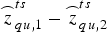 ${\mathop{z}\limits^{\frown}} _{qu,1}^{ts} - {\mathop{z}\limits^{\frown}} _{qu,2}^{ts} $
. It thereby allows us to make the best trade off between the searching efficiency that depends on the lengths of the search ranges, and the empirical IAR success rate.
For each pair of
 $\tilde z_1$
and
 $\tilde z_2$
within the search ranges, we compute the following test value,
 $$d_{IF} = \left \vert {{\mathop{z}\limits^{\frown}} _{qu,IF}^{ts} - {\tilde z}_{IF}} \right \vert $$
where
 $\tilde z_{IF}$
denotes the ionosphere-free linear combination of
 $\tilde z_1$
and
 $\tilde z_2$
. The pair which gives rise to the smallest d
IF
is accepted as a final solution, unless d
IF
≥ d
max with d
max a user-defined value (by default we set d
max = 0.1 cycles). After that, we re-estimate the dual-frequency float DD ambiguities for the rest of the satellite-pairs and resolve them iteratively.
5. NUMERICAL TESTS
In this section we initially assess the accuracy of the atmospheric delays, determined by PPP using our in-house developed software from a batch of two hour GPS data sets under various atmospheric conditions. Also, we comparatively evaluate the performances of our proposed QIF and the standard WN strategies for GPS long-baseline IAR.
5.1. Experimental data preparation and processing
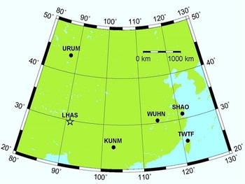
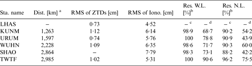
Our numerical tests chose the dual-frequency GPS data collected by six static receivers managed by the IGS on day 96 of 2003 with 30-second time resolution; this is an arbitrary choice. Figure 1 shows the geographic distribution of all the receivers, as well as their four character names. We define a total of five long-baselines by specifying the LHAS as the pivot receiver. We summarise the distances of all these long-baselines in the second column of Table 1.
Geographic distribution of the GPS receivers involved in our numerical tests. When forming the long-baselines, LHAS is specified as the pivot receiver, whose distances to the remaining rover receivers range from almost 3,000 km (TWTF), down to roughly 1,200 km (KUNM).

Overview of the results obtained from our numerical tests.

a with respect to the LHAS
b percentage of residual ambiguities within [-0·5, 0·5] cycles
c based on the QIF strategy with the aid of PPP-derived atmospheric delay constraints
d based on the WN strategy
We divide the daily GPS data for each receiver into 12 two hour segments. By means of the least-square estimator, both our PPP and DD data processing are subsequently conducted on a per segment basis. The main reason for processing two hours’ data is that it usually takes more than one hour for various PPP solutions (especially the SIDs) to be sufficiently accurate.
The basic settings adopted for our data processing are as follows. The necessary products of the satellite clock offsets and orbit as well as consistent position of the pivot receiver LHAS are acquired from the IGS. The cut-off elevation angle is chosen to 5 (20) degrees for the PPP (DD data processing). Elevation-dependent weighting is applied with the zenith-referenced formal precision of the ZD code and carrier-phase data set to 30 and 0·3 centimetres. A random walk sigma is set to 0·03 mm/s (0·3 mm/s) when estimating the ZTDs (SIDs).
5.2. Accuracy assessment of PPP-derived atmospheric delays
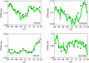
On the day of the experiment, IGS offered the ZTD products for all our experimental receivers except the SHAO, with millimetre-level accuracy and two hour time resolution. Using these available ZTD products as ground-truths, we would be able to assess the quality of our PPP-derived ZTDs for every experimental receiver.
The ZTDs provided by PPP with 30-second time resolution for four receivers with different geodetic heights (green lines), and their ground truths delivered by the IGS with 2-hour time resolution (black triangles), in metres.

Figure 2 depicts, respectively, the PPP-derived ZTDs (green lines) as well as the IGS ZTD products (black triangles) for four receivers LHAS/URUM/TWTF/KUMN. Our results confirm the dependence of troposphere effect on the geodetic height. This is clearly visible for the LHAS (TWTF) receiver with largest (smallest) geodetic height and smallest (largest) overall size of the ZTDs. Furthermore, we notice that the diurnal variability of the ZTDs behaves differently among receivers, mainly due to the site-specific troposphere conditions.
At the epochs when the IGS ZTD products are available, we differenced them with respect to the PPP-derived ZTDs and then computed the Root Mean Squares (RMS). We follow this procedure for all the receivers except SHAO and summarise the computed RMS in the third column of Table 1. From the analysis, it emerges that PPP could provide the ZTDs with better than two centimetre accuracy using only two hours’ GPS data. Since its position has been assumed to be known, the PPP-derived ZTDs for the pivot receiver LHAS therefore correspond to the smallest RMS (0·73 centimetres).
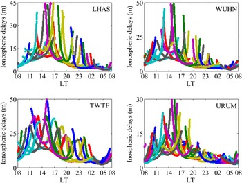
As we mentioned before, the PPP-derived SIDs are biased by the scaled receiver as well as satellite DCBs. Together with the Global Ionosphere Maps (GIM), IGS also makes the values of DCBs for a global network of receivers (including all our experimental receivers) and GPS satellites available (Hernández-Pajares et al., Reference Hernández-Pajares, Juan, Sanz, Orus, Garcia-Rigo, Feltens, Komjathy, Schaer and Krankowski2009). We apply these values to the SIDs estimated by PPP for four receivers LHAS/WUHN/TWTF/URUM, and depict the results that are DCB-free in Figure 3 as a function of local time (LT = UTC + 8).
The DCB-free SIDs (in metres) provided by PPP for four receivers at different latitudes, as a function of Local Time (LT). Different colours correspond to different satellites.

Figure 3 allows us to understand the dependence of ionosphere effect on the Local Time (LT) and also on the latitude. Basically, the diurnal variability of the SIDs observed by all the receivers is very typical: the SIDs reach diurnal maximum around the local noon (14:00 LT); after that, they show a gradual fall and reach diurnal minimum shortly after the local midnight (02:00 LT). In addition, with respect to the two receivers LHAS and URUM at approximately the same longitude, the largest difference of SIDs between them occurs at local noon and can amount to about 15 metres. This is most likely due to the distinct ionospheric conditions represented by the latitudes at these two receivers.
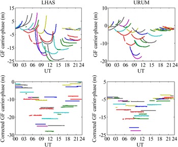
Because of their inadequate accuracy, the GIMs would be inappropriate to act as the ground truths of our PPP-derived SIDs. To avoid this limitation, we develop an idea that could fulfil the accuracy assessment of the PPP-derived SIDs without requiring any externally provided ground truths. We explain the basic principle of our idea as follows. For a given receiver, we apply the PPP-derived SIDs as corrections to the very precise ZD geometry-free carrier-phase data. In the ideal case when these “corrections” are free from errors, the corrected ZD geometry-free carrier-phase data would contain only one constant (but unknown) ambiguity for every continuous satellite pass. We compute, per satellite pass, the standard deviations of the corrected ZD geometry-free carrier-phase data and use their mean value as the RMS of the PPP-derived SIDs.
To exemplify our idea described above, we show in Figure 4 the ZD geometry-free carrier-phase data collected by receivers LHAS and URUM, before and after applying the PPP-derived SIDs. We see that a large amount of the ionospheric effects underlying the geometry-free carrier-phase data can indeed be well compensated. The corrected geometry-free carrier-phase data for most of the satellite passes stay very close to constants, thus implying quite minor errors in the “corrections”.
We present the values of the RMS of PPP-derived SIDs for all the receivers in the fourth column of Table 1. It follows that the PPP is able to provide SIDs with accuracy better than 10 centimetres using two hours’ GPS data under various ionospheric conditions. Again, the minimum RMS (4·52 centimetres) occurs for the pivot receiver LHAS, thanks to treating its position as completely known.
The zero-differenced, geometry-free carrier-phase data collected by receivers LHAS (left panels) and URUM (right panels), in metres: before and after applying the PPP-derived SIDs. Different colours correspond to different satellites.

5.3. Performance evaluation of proposed QIF strategy
When estimating the float DD ambiguities for the five long-baselines defined by us, we make use of the RMS values of PPP-derived ZTDs (SIDs) given in Table 1 to determine the uncertainties of the tropospheric (ionospheric) constraints. We assume, rather conservatively, the RMS of PPP-derived ZTDs for receiver SHAO that is unavailable, to be two centimetres.
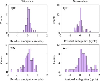
We attempt to resolve the estimated float DD ambiguities with our proposed QIF strategy and compare the results of relevance with respect to those obtained from the standard WN strategy. Our comparison mainly investigates the so-called residual ambiguities, defined as the deviations between the float ambiguities and their ground truths, for both the wide-lane and the narrow-lane linear combinations. Note that we process the daily GPS data of all the long-baselines considered here with the Bernese GPS software to determine the integer ground truths of the DD ambiguities using the WN strategy.
We include in the fifth (sixth) column of Table 1, for all the long-baselines, the percentages of wide-lane (narrow-lane) residual ambiguities that reside between –0·5 and +0·5 cycles, which actually represent the empirical success rates of wide-lane (narrow-lane) IAR using the rounding method (Teunissen, Reference Teunissen1998b). It follows that use of integer rounding method, the QIF, in all the cases can resolve at least 98% (88%) of wide-lane (narrow-lane) ambiguities. However, under the same condition, the WN is only able to resolve at most 90·6% (76·6% on average) of the wide-lane ambiguities and 75·5% (55·2% on average) of the narrow-lane ones.
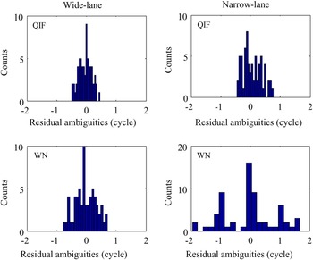
Complementarily, we also would like to focus our attention on the remaining residual ambiguities with absolute values greater than +0·5 cycles, resolution of which has to refer to the searching rather than the integer rounding method. We mainly investigate the frequency of their occurrence, as well as their actual sizes. Both measures combined would be able to quantitatively describe the searching efficiency. Our QIF simultaneously resolves the dual-frequency float DD ambiguities by means of searching, whereas the WN relies on the searching only for the narrow-lane IAR. To realise a fair comparison between both strategies, we will limit our analysis here merely to the narrow-lane residual ambiguities. We depict in Figures 5 and 6 the residual ambiguities computed for two long-baselines, LHAS-WUHN and LHAS-URUM, respectively (the wide-lane results are also involved for completeness sake).
The wide-lane and narrow-lane residual ambiguities obtained from the proposed QIF (upper panels) and the WN (lower panels) strategies, in cycles: LHAS-WUHN long-baseline with length of 2,228 km.

Considering first of all the QIF-based narrow-lane residual ambiguities shown in Figure 5 for long-baseline LHAS-WUHN, fewer than one tenth (9·7%) have absolute values exceeding +0·5 cycles. In addition, only one exceeds one cycle, whose search range should therefore be defined as [–2, 2] cycles containing five integer candidates. In contrast, we find that 40% of the WN-based narrow-lane residual ambiguities stay outside of the range [–0·5, 0·5] cycles. More than ten with absolute values surpassing one cycle need to be assigned with search ranges of [–2, 2] cycles. The situation for the other long-baseline LHAS-URUM is somewhat similar (see Figure 6): we only need to resolve 9·1% of the QIF-based narrow-lane residual ambiguities based on searching. Their search ranges are all [–1, 1] cycles containing at most three integer candidates. However, the absolute values of 56·1% of the WN-based narrow-lane residual ambiguities are greater than +0·5 cycles. Moreover, the search ranges of tens of them correspond to [–2, 2] cycles.
6. CONCLUDING REMARKS
GPS long-baseline setup is a very useful tool to serve a wide range of geodetic and geodynamic applications. Resolution of the DD ambiguities into integers (IAR) is always essential, in order to take fully advantage of the very precise carrier-phase data. However, the bottleneck problems that inhibit fast and successful GPS long-baseline IAR originate from the presence of very significant atmospheric delays in the DD data. Because of this, two sophisticated strategies adopted by the Bernese GPS software, name the QIF and the WN, need to process at least 8–24 hours’ GPS data to ensure reliable IAR.
The wide-lane and narrow-lane residual ambiguities obtained from the proposed QIF (upper panels) and the WN (lower panels) strategies, in cycles: LHAS-URUM long-baseline with length of 1,597 km.

With the goal of speeding up the QIF-based IAR, we propose in this contribution the following procedures. We first turn to the PPP method to estimate the ZTDs/SIDs for the pivot and the rover receivers, respectively, using their ZD GPS data. Afterwards, we formulate the resulting ZTDs (SIDs) into the tropospheric (ionospheric) constraints with proper uncertainties, such that they can be used as pseudo-observables, together with the original DD data, to generate more precise float DD ambiguities for the QIF. Using a batch of two hours of GPS data sets collected by six static receivers under various atmospheric conditions, we verify the very promising accuracy of the PPP-derived ZTDs (RMS <2 centimetres) and SIDs (RMS <10 centimetres). Also, we conclude that, thanks to the contribution of the introduced atmospheric constraints, the IAR performance achieved by our proposed QIF, in terms of searching efficiency as well as empirical success rate, is much better than that by the WN.
Finally, we have to emphasise that the generality of our quantitative conclusions drawn from the numerical tests is currently limited to the static GPS long-baseline data analysis. To achieve comparable IAR performance, longer observation time spans are required when we apply the proposed QIF strategy to the kinematic GPS long-baselines. The feasibility of our proposed QIF strategy depends, to a very large extent, on the ability of PPP offering the high-accuracy ZTDs/SIDs, and thus may be unfavourable in a few cases: the ZTDs/SIDs estimated by PPP under extreme space weather situations would be less accurate or even hardly possible; the low quality orbits and clocks of eclipsing GPS satellites, once undetected, might impair the reliability of PPP solutions (Kouba, Reference Kouba2009).
ACKNOWLEDGMENTS
This work was supported by the National Natural Science Foundation of China (41231064), the National Basic Research Program of China (2012CB825604), and the CAS/SAFEA International Partnership Program for Creative Research Teams (KZZD-EW-TZ-05). We also would like to acknowledge the International GNSS Service (IGS) for providing the GPS data and products used in our experiment.