

Introduction
Over the past century, estimation of fossil diversity (most commonly, taxonomic richness) and its variations through geologic time has been a major paleontological research axis, leading to fundamental discoveries and significant progress in the knowledge of Phanerozoic biodiversity change (Phillips Reference Phillips1860; Harland et al. Reference Harland, Holland, House, Hughes, Reynolds, Rudwick, Satterthwaite, Tarlo and Willey1967; Raup Reference Raup1972, Reference Raup1991a; Ager Reference Ager1976; Sepkoski Reference Sepkoski1978, Reference Sepkoski1993, Reference Sepkoski2002; Sepkoski et al. Reference Sepkoski, Bambach, Raup and Valentine1981; Benton Reference Benton1993). Unfortunately, past biodiversity estimates are very likely to be plagued, at least for some clades and time intervals, by many sampling and analytical biases and drawbacks (Raup Reference Raup1976; Bambach Reference Bambach1977; Koch Reference Koch1978; Signor and Lipps Reference Signor and Lipps1982; Benton and Ayala Reference Benton and Ayala2003; Alroy et al. Reference Alroy, Aberhan, Bottjer, Foote, Fürsich, Harries, Hendy, Holland, Ivany, Kiessling, Kosnik, Marshall, McGowan, Miller, Olszewski, Patzkowsky, Peters, Villier, Wagner, Bonuso, Borkow, Brenneis, Clapham, Fall, Ferguson, Hanson, Krug, Layou, Leckey, Nürnberg, Powers, Sessa, Simpson, Tomašových and Visaggi2008), including rock preservation and decay, and thus variation in fossil availability through time (Smith Reference Smith2001; Crampton et al. Reference Crampton, Beu, Cooper, Jones, Marshall and Maxwell2003; Benson et al. Reference Benson, Butler, Lindgren and Smith2009); variation in the rate of fossil preservation (Foote Reference Foote2001); unequal numbers of collections and systematicians per clade and through time and varying taxonomic practices, opposing splitters and lumpers (Benton Reference Benton2010; Benton et al. Reference Benton, Dunhill, Graeme and Marx2011). Even if most of these issues have long been acknowledged, perception and understanding of them have varied greatly over the last decades. For instance, variations of sampling effort through geologic time, once seen as a marginal issue, is now regarded as a major bias affecting taxonomic-richness reconstructions—a bias possibly accommodated through correction methods such as random subsampling (Alroy et al. Reference Alroy, Aberhan, Bottjer, Foote, Fürsich, Harries, Hendy, Holland, Ivany, Kiessling, Kosnik, Marshall, McGowan, Miller, Olszewski, Patzkowsky, Peters, Villier, Wagner, Bonuso, Borkow, Brenneis, Clapham, Fall, Ferguson, Hanson, Krug, Layou, Leckey, Nürnberg, Powers, Sessa, Simpson, Tomašových and Visaggi2008, Reference Alroy2010a).
Apart from these well-known and still heavily debated potential sources of biases requiring the use of appropriate sampling and/or computational correction methods, the methods used in constructing paleontological data sets and biozonations may also generate potential biases (Raup Reference Raup1972, Reference Raup1976; Sepkoski Reference Sepkoski1981; Alroy et al. Reference Alroy, Marshall, Bambach, Bezusko, Foote, Fürsich, Hansen, Holland, Ivany, Jablonski, Jacobs, Jones, Kosnik, Lidgard, Low, Miller, Novack-Gottshall, Olszewski, Patzkowsky, Raup, Roy, Sepkoski, Sommers, Wagner and Webber2001, Reference Alroy, Aberhan, Bottjer, Foote, Fürsich, Harries, Hendy, Holland, Ivany, Kiessling, Kosnik, Marshall, McGowan, Miller, Olszewski, Patzkowsky, Peters, Villier, Wagner, Bonuso, Borkow, Brenneis, Clapham, Fall, Ferguson, Hanson, Krug, Layou, Leckey, Nürnberg, Powers, Sessa, Simpson, Tomašových and Visaggi2008; Escarguel and Bucher Reference Escarguel and Bucher2004; Foote Reference Foote2005, Reference Foote2007). Indeed, all fossil-based studies of biodiversity variations through geologic time fundamentally rely on the compilation of taxonomic occurrences within successive time intervals (i.e., biozones), thus requiring the preliminary construction of a time-calibrated biochronological framework. By definition, whatever the biochronological methodology used (e.g., concurrent-range zones, interval zones, association zones, unitary associations; Smith Reference Smith1816; d’Orbigny Reference d’Orbigny1842–1849; Oppel 1Reference Oppel856–1858; Buckman Reference Buckman1893; Cope Reference Cope1993, Reference Cope1994), a biozonation is a set of successive but not necessarily contiguous discrete time intervals of unequal duration. As far as biodiversity is concerned, such “time discretization” has strong consequences, as it potentially presents taxa as falsely co-occurring within biozones, and thus artifactually modifies the biodiversity signal; the longer the biozone, the larger the expected absolute and relative amount of falsely co-occuring taxa. Incidentally, we note that biochronological methods based on the maximal-association principle (e.g., the unitary associations method; Guex Reference Guex1991) explicitly exclude such false co-occurrences from the constructed biozonation, thus maximizing biochronological correlation accuracy with the logical drawbacks of poor representation of genuine biodiversity variations and very low time coverage (e.g., maximal association zones classically represent no more than 30% of the time covered by the biozonation; Escarguel and Bucher Reference Escarguel and Bucher2004: Figs. 4, 8, 15). From the point of view of the time record of biodiversity changes, an efficient biozonation method should obviously maximize the total amount of time included in successive biozones to capture the biodiversity history in its entirety. Nevertheless, such a contiguous biozones framework will necessarily involve an increase of false co-occurrences, potentially distorting the genuine biodiversity signal (Supplementary Fig. S1).
Facing this dilemma, our main objective with this work was to explore the way a contiguous biozones framework, leading to the discretization into successive time intervals of unequal durations of a basically continuous-time signal, may affect our knowledge of fossil biodiversity changes, regardless of any other potential sources of bias. As far as we are aware, little is currently known about the influence of biozonation construction (and therefore time discretization) on biodiversity estimation. Only a small number of authors have observed or taken into account the potential biasing effect of the duration of time intervals on taxonomic richness (Raup Reference Raup1976; Sepskoski Reference Sepkoski, Bambach, Raup and Valentine1981; Van Valen Reference Van Valen1973; Bambach Reference Bambach1999; Foote Reference Foote2000, Reference Foote2005; Alroy et al. Reference Alroy, Marshall, Bambach, Bezusko, Foote, Fürsich, Hansen, Holland, Ivany, Jablonski, Jacobs, Jones, Kosnik, Lidgard, Low, Miller, Novack-Gottshall, Olszewski, Patzkowsky, Raup, Roy, Sepkoski, Sommers, Wagner and Webber2001, Reference Alroy, Aberhan, Bottjer, Foote, Fürsich, Harries, Hendy, Holland, Ivany, Kiessling, Kosnik, Marshall, McGowan, Miller, Olszewski, Patzkowsky, Peters, Villier, Wagner, Bonuso, Borkow, Brenneis, Clapham, Fall, Ferguson, Hanson, Krug, Layou, Leckey, Nürnberg, Powers, Sessa, Simpson, Tomašových and Visaggi2008; Lu et al. Reference Lu, Yogo and Marshall2006). For instance, Alroy et al. (Reference Alroy, Aberhan, Bottjer, Foote, Fürsich, Harries, Hendy, Holland, Ivany, Kiessling, Kosnik, Marshall, McGowan, Miller, Olszewski, Patzkowsky, Peters, Villier, Wagner, Bonuso, Borkow, Brenneis, Clapham, Fall, Ferguson, Hanson, Krug, Layou, Leckey, Nürnberg, Powers, Sessa, Simpson, Tomašových and Visaggi2008) time-standardized their fossil data set by counting generic richness within homogeneous 11-Myr-long slices, thus removing the effect of heterogeneity of time interval duration that can potentially lead to the overaccumulation of falsely co-occurring taxa within the longest time intervals. Unfortunately, this method removes the effect of heterogeneity of time interval duration at the expense of analytic time resolution and further increases false co-occurrences within time intervals.
In practice, the original, genuine continuous-time biodiversity history is obviously unknown to paleontologists, making a direct comparison between the “true” (continuous-time) and time-discretized signals impossible. A straightforward and efficient solution is computer simulation involving generation of a continuous-time biodiversity history, followed by construction of a discrete-time data set from that history based on a superimposed contiguous biozones framework, extraction of the biodiversity curve from this discretized data set, and finally, comparison of the original, continuous-time biodiversity signal to this discrete-time one. As is usual in such simulation approaches, a sensitivity analysis allows interpretation of the relationship between the continuous-time and discrete-time curves in terms of several key parameters such as the number of simulated taxa, their mean longevity, or the mean duration of biozones with respect to the total length of the simulated time interval. For instance, it seems intuitive that the longer the mean taxonomic longevity and the shorter the mean biozone duration, the closer the discretized biodiversity signal will be to the original one. Nevertheless, the relative effect of these two parameters on the quality of the resulting correlation is far less obvious, an issue that is addressed through sensitivity analysis.
From this point of view, an additional key parameter is particularly worth investigating: the potential relationship between taxonomic turnover dynamics and the time-location in time of biozone boundaries. Contiguous biozones frameworks as considered here usually result from the exclusive use, or a more or less explicit mixing, of four major types of biozones (range, interval, assemblage, and acme biozones). All of them are defined by the presence (eventually abundance) and/or absence, and thus the distribution, origination, and/or extinction, and coexistence or mutual exclusion, of taxa (Hedberg Reference Hedberg1976; Cope Reference Cope1993, Reference Cope1994; Rey Reference Rey1997; Woodburne Reference Woodburne2012). In this context, the interdependence of biozone boundaries and taxonomic turnover dynamics must be considered. Biozone boundaries within a given paleontological data set may have been established within time spans of high taxonomic turnover (resulting in a noticeable accumulation of origination and/or extinction events), with biozone centers thus corresponding to relatively lower turnover periods. However, biozone boundary locations may be formally decoupled from taxonomic turnover dynamics (Foote Reference Foote1994; Alroy Reference Alroy1998, Reference Alroy2008; Woodburne Reference Woodburne2012), even more so when defined by the origination and/or extinction of a very few index taxa whose individual evolutionary histories do not necessarily reflect the turnover dynamics of the whole assemblage. Incidentally, independence between turnover dynamics and the location of biozone boundaries can also be expected when studying biodiversity changes of a given taxonomic group using a biozonation built on another taxonomic group with a distinct biodiversity history. In addition to the two extreme cases of perfect dependence or independence between origination/extinction and biozone boundary location (corresponding to Foote’s [Reference Foote2005] pulsed and continuous origination and extinction models), we also investigate here intermediate cases across a spectrum of potential relationships, ranging from a strong dependence to a total independence between biozone boundary location and taxonomic turnover dynamics.
Based on these simulation results, we propose a straightforward algorithm that generates a virtually continuous-time averaged curve of taxonomic richness, taxonomic origination, or extinction rate based on a discrete-time taxonomic-richness data set as customarily constructed by paleontologists. Starting from the information available in any paleontological data set (i.e., presence/absence of taxa within discrete time intervals), this algorithm randomly draws for each sampled taxon a continuous-time origination and extinction age within the corresponding time intervals. Building on the simulation approach detailed below, we are able to compare the time-discretized and back-transformed, virtually continuous-time reconstructed biodiversity histories against the “true,” original (continuous-time) one. In spite of the simplicity of this algorithm, we show that the averaged, virtually continuous-time biodiversity history reconstructed in this way from the time-discretized data set fits the original history much more closely than the time-discretized one, even when the data set settings are particularly adverse to an accurate time-discretized reconstruction. The source code (written in R) that performs such a back-transformation for any real paleontological data set associated with a time-calibrated biozonation is available in the Supplementary Material (http://dx.doi.org/10.5061/dryad.g9k46).
Materials and Methods
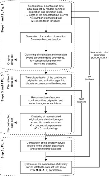
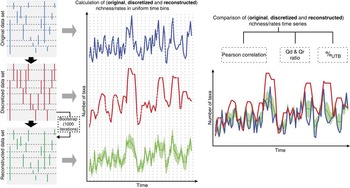
The simulation approach developed here to explore the relationships between “true” (continuous-time), time-discretized, and finally, back-transformed (virtually continuous-time) reconstructed diversity curves relies on five successive steps (Fig. 1):
-
1. generation of an initial, continuous-time data set of temporal distribution of taxa by random sorting of their origination and extinction ages based on a specified distribution of taxon longevity;
-
2. random generation of a biozonation (i.e., ages of contiguous biozone boundaries) based on a specified distribution of biozone duration, and clustering of taxon origination and extinction ages around their closest biozone boundaries (leading to the original data set);
-
3. time discretization of the original data set, that is, transformation of continuous origination–extinction time intervals for each taxon into discrete occurrences within biozones (leading to the discretized data set);
-
4. random reconstruction of new, virtual origination/extinction ages for each taxon within its first and last occurrence biozone, respectively (leading to the reconstructed data set); and
-
5. comparison of the diversity curves related to the original data set (obtained at the end of step 2), the discretized data set (end of step 3), and the reconstructed data set (end of step 4).
Flowchart of the simulation approach detailed in Figs. 2–4. The first main step of the simulation (Fig. 2) leads to the generation of an original, continuous-time data set of taxon origination and extinction based on the T, N, M, D, and A control parameters. The second main step (Fig. 3) leads to the time-discretization of the original data set into a discretized data set, which is then back-transformed into a virtually continuous-time reconstructed data set (depending on control parameter C). The third main step (Fig. 4) refers to the comparison of the original, discretized, and reconstructed time series based on different comparison metrics.

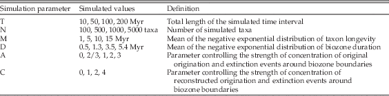
This five-step simulation procedure relies on six control parameters introduced in Table 1 and detailed below. Because these parameters are partly redundant, their selection could have been simplified by using, for example, parameters standardized with respect to mean taxon duration. Nevertheless, we favored the use of raw, unstandardized parameters to keep the interpretation as realistic and intuitive as possible. This makes the comparison and discussion of the relationships between the simulation results and the analysis of real paleontological data sets easier and more straightforward. In any case, working on standardized parameters would not change the results, leading to the identification of the very same bias effects and first-order control parameters.
Simulated values and definitions for the six simulation parameters used in this study.

Step 1. Generation of an Initial Data Set
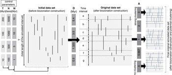
The first step relies on the random generation, for each simulated taxon, of an origination and an extinction age (in Ma, defined on a yearly basis), based on three control parameters: T, N, and M (see Table 1 for term definitions, Fig. 2). Use of the negative exponential distribution as a model distribution for taxon longevity is based on Van Valen’s (Reference Van Valen1973) observation of log-linearity of poly-cohort survivorship curves.
First main step of the simulation, leading to the original data set. T, total length of the simulated time interval (in Myr); N, number of simulated taxa; M, mean taxon longevity: D, mean biozone duration; A, intensity of origination and extinction clustering around biozone boundaries.

To generate diversity curves under a steady-state dynamic equilibrium and to avoid edge effects (artifactual increase and decrease of taxonomic richness at the beginning and end of the simulated time interval, respectively), for each simulated taxon i, the longevity L i was first randomly generated within a negative exponential distribution of mean M, then the origination age o i was uniformly drawn between 0 and T+L i Ma, and finally, the extinction age (falling between −L i and T) was calculated as e i =o i −L i . In this way, all simulated taxa have at least part of their respective ranges falling within the [0; T] simulated time interval. Finally, this initial data set is retained for the next simulation step only if the distribution of simulated longevities fits well enough with its parent negative exponential model distribution, as assessed through computation of the coefficient of determination (R 2 ) between the two distributions (lower “acceptable” limit for R 2 ranging from 0.85 to 0.95 as N increases from 100 to 5000).
Step 2. Construction of a Contiguous Biozones Framework and Origination/Extinction Clustering around Biozone Boundaries
The initial data set resulting from step 1 consists of N taxa with origination and extinction ages randomly distributed along a continuous-time axis defined on a yearly basis, whereas fossil taxonomic-richness information is usually recorded in a succession of discrete time intervals (biozones or even geologic stages) with boundaries customarily defined by one or several roughly contemporaneous taxon origination(s) and/or extinction(s) (Hedberg Reference Hedberg1976; Cope Reference Cope1993, Reference Cope1994; Rey Reference Rey1997; Woodburne Reference Woodburne2012). To simulate the information provided by the fossil record, a biozonation (i.e., a succession of biozone boundaries) is first established independent of the distribution of originations and extinctions in the initial data set by random generation of successive biozone durations (Fig. 2) within a negative exponential distribution with a mean set between D=0.5 (as observed, e.g., for Cenozoic biozonations based on rapidly-evolving and short-ranging organisms such as planktonic foraminifera; Huber Reference Huber1992; Cope Reference Cope1993) and 5.4 Myr (corresponding to the average duration of Phanerozoic geologic stages; Gradstein et al. Reference Gradstein, Ogg, Schmitz and Ogg2012) (Table 1).
As a biozone (or stage) boundary is usually defined based on origination and extinction events of geographically widespread taxa, high taxonomic turnovers may occur around biozone/stage boundaries. To mimic such acute concentrations of taxon originations and extinctions around biozone/stage boundaries, origination and/or extinction ages for each simulated taxon can be recalculated by random generation from a normal distribution centered on the boundary closest to the initial age (Fig. 2). The standard deviation (SD) associated with this normal distribution controls the strength of concentration of origination/extinction events around the boundaries: the lower the SD, the higher the concentration effect. For each taxon origination or extinction age, SD is computed from the half-duration of the biozone/stage before or after the target boundary (randomly chosen with equal probability), weighted by a constant A empirically fixed between 2/3 (weakest concentration effect) and 3 (strongest concentration effect) (Table 1). More specifically:
 $${\rm SD}\,{\equals}\,\left\{ {\matrix{ {{{t_{{i{\plus}1}} {\minus}t_{i} } \over {2{\rm A}}}{\rm }\left( 1 \right)} \cr {{{t_{i} {\minus}t_{{i{\minus}1}} } \over {2{\rm A}}}{\rm }\left( 2 \right)} \cr } } \right\}, {\rm with}\,prob\left( 1 \right)\,{\equals}\,prob\left( 2 \right)\,{\equals}\,0.5$$
with t i being the age of the target boundary, and t i+1 and t i−1 the ages of the boundaries immediately before and after the target boundary, respectively. Several simulations were performed with various origination/extinction concentration intensities, from no concentration (i.e., origination and extinction ages remain unchanged with respect to the initial data set) to a very strong concentration effect (A=3). The initial data set resulting from step 1, combined with its superimposed biozonation, with taxon origination and extinction ages more or less clumped around biozone boundaries, ultimately constitutes the original data set (Fig. 2).
Step 3. Transformation of a Continuous-Time Record into a Discrete-Time Record
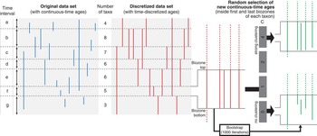
The original data set resulting from step 2 still records taxon occurrences along a continuous-time axis and thus needs to be transformed into a discrete-time record corresponding to the presence/absence of each simulated taxon within each simulated biozone. Therefore, during this third step, the original data set is discretized to mimic a data set as empirically constructed from the fossil record: a paleontological data set of taxon occurrences within successive biozones/stages (Fig. 3). By comparing the continuous-time origination and extinction ages with the location of biozone boundaries, information about the presence or absence of each taxon within each biozone is obtained and recorded into a discretized data set in which the exact origination and extinction numerical ages are lost and replaced by the lower boundary of the biozone where the taxon originates and the upper boundary of the biozone where it becomes extinct, respectively. From this discretized data set, a new diversity stepping curve (as classically obtained from the fossil record) is computed and ultimately compared with the diversity curve corresponding to the original data set (see step 5).
Second main step of the simulation, corresponding to the time-discretization of the original data set (→ discretized data set) and then back-transformation of the discretized data set into a virtually continuous-time reconstructed data set. C, intensity of the clustering of reconstructed taxon origination and extinction around biozone boundaries.

Step 4. Reconstruction of Virtual Origination/Extinction Ages from the Discretized Data Set
Based on the discretized data set, the next step consists of recalculating new continuous-time origination and extinction ages randomly selected within the first (origination) and the last (extinction) biozone in which each taxon occurs (Fig. 3). For the very same reasons as those discussed for step 2, this random generation of new origination/extinction ages can be performed by uniformly drawing from the lower to the upper boundaries of the target biozone (no concentration of origination/extinction events around the biozone boundaries) or can be concentrated around the boundaries. Concentration of origination/extinction ages is obtained here through the use of a logistic model:
 $$t_{{{\rm new}}} {\equals}{{t_{{{\rm upp}}} {\minus}t_{{{\rm low}}} } \over {1{\plus}{\rm e}^{{{\minus}{\rm C}\left( {10x{\minus}5} \right)}} }}{\plus}t_{{{\rm low}}} $$
where t new is the new continuous-time origination/extinction age; t low and t upp are the lower and upper boundary ages of the target biozone, respectively; x is a [0, 1] uniform random variate (x=0 gives t new=t low, and x=1 gives t new=t upp); and C modulates the steepness of the sigmoidal shape of the logistic function, and thus the intensity of the concentration of origination/extinction events around the boundaries (the larger C is, the steeper the logistic function and the higher the concentration effect; the closer C is to 0, the closer this model is to a uniform random drawing of t new between t low and t upp) (Table 1). We use here a logistic distribution model between two successive biozone boundaries rather than a normal distribution model centered on a given biozone boundary as used in step 2) for two complementary reasons:
-
∙ During step 2 (computation of original origination and extinction ages), the biozone boundary closest to the initial origination or extinction age is used as a “bilateral attractor” for the computation of a new origination or extinction age. This new age can equiprobably fall on both sides of the target boundary, implying that the original age has a 50% chance to fall outside the biozone limits, including the initial age. During step 4 (here), the reconstructed origination or extinction age (t new) must be calculated within the biozone in which the taxon originates or becomes extinct, suggesting that its lower and upper limits are the target biozone boundary ages (t low and t upp), a situation typically corresponding to a logistic distribution model bounded between t low and t upp;
-
∙ As the exact distribution model(s) for the original ages around biozone boundaries is/are unknown in real case studies, it seems more sensible to use different distribution models in steps 2 and 4, so that the improvement resulting from the back-transformation algorithm (step 4) does not rely on the exact identity between the distribution models used in the two steps of the simulation.
The diversity curve related to the reconstructed data set resulting from this procedure idiosyncratically depends on the randomly recalculated origination and extinction ages, making its direct comparison to the curves corresponding to the original and discretized data sets of little (if any) interest. This recalculation procedure is therefore coupled with a Monte-Carlo simulation to estimate an “average reconstructed curve” (Fig. 3): 1000 reconstructed data sets are independently obtained from the same discretized data set, finally allowing the computation of an average reconstructed diversity curve and its associated 95% confidence interval (Fig. 4).
Third main step of the simulation, corresponding to the comparisons of the resulting original, discretized, and reconstructed time series through three complementary indices: Pearson correlation, Qd, and Qr ratios (mean ratio between discretized [Qd] or reconstructed [Qr] taxonomic richness/rates value and original taxonomic richness/rate value), and %UTB (percentage of UTBs where the original taxonomic richness/rate value falls within the 95% confidence interval of the reconstructed taxonomic richness/rate).

Step 5. Comparison of the Original, Discretized, and Average Reconstructed Diversity Curves
The diversity histories suggested by the original (end of step 2), discretized (end of step 3), and average reconstructed (end of step 4) data sets are finally compared by focusing on two complementary metrics: taxonomic richness and taxonomic origination and extinction rates (Fig. 4). The taxonomic richness/rate time series related to each of these three data sets are calculated within uniform time bins (UTBs) with duration dependent on the mean biozone duration (D) used in the simulation. Indeed, using either a very small UTB value for a data set with a large D value, or a large UTB value for a small-D data set would generate spurious effects artifactually increasing or decreasing the estimated quality of the relationships between the three diversity histories. Therefore, with D=5.4 and 3.5 Myr, UTB=2 Myr is used; with D=1.325 Myr, UTB=1 Myr; and with D=0.5 Myr, UTB=0.1 Myr.
Two distinct strategies are used to compute the discretized and reconstructed taxonomic-richness curves, depending on whether singletons (i.e., taxa restricted to a single biozone/stage, and thus taxa that are not boundary crossers) are taken into account or not (Foote Reference Foote2000; Alroy et al. Reference Alroy, Marshall, Bambach, Bezusko, Foote, Fürsich, Hansen, Holland, Ivany, Jablonski, Jacobs, Jones, Kosnik, Lidgard, Low, Miller, Novack-Gottshall, Olszewski, Patzkowsky, Raup, Roy, Sepkoski, Sommers, Wagner and Webber2001). Indeed, the richness values calculated for successive biozones/stages may vary independently with respect to the original richness values due to several biasing factors such as variations in preservation rates and/or sampling effort, monographic or Lagerstätte effects, or even biozone/stage duration—the longer the time interval, the more likely it is to contain a large proportion of singletons. Therefore, ignoring taxa that originated and became extinct in the same time interval may help to at least partially circumvent some of those biases (Barry Reference Barry1995; Bambach Reference Bambach1999) and thus improve the quality of the relationships between the three diversity histories.
In addition to the computation and comparison of taxonomic-richness time series, we also compute and compare the time series of taxonomic origination and extinction rates associated with the original, discretized, and average reconstructed data sets. Indeed, such taxonomic rates are frequently computed alongside taxonomic-richness time series to estimate the underlying richness- and time interval–standardized proportional changes in origination and extinction dynamics. This makes it worth investigating their relative behavior with respect to the time-discretization procedure as well as to the reconstruction algorithm. We use singleton-free Foote’s (Reference Foote2000) per capita-Myr origination
 $\left( {\hat{p}} \right)$
and extinction
 $\left( {\hat{q}} \right)$
rates
 $$\hat{p}\,{\equals} {{{\minus}\ln \left( {{{Nbt} \over {NFt{\plus}Nbt}}} \right)} \over {\delta t}}\,{\rm and}\,\hat{q}\,{\equals}{{{\minus}\ln \left( {{{Nbt} \over {NbL{\plus}Nbt}}} \right)} \over {\delta t}}$$
where N bt is the number of taxa that cross both bottom and top biozone/stage boundaries for the discretized data set or bottom and top UTB boundaries for the original and reconstructed data sets; N Ft is the number of taxa originating within the biozone/stage or UTB and crossing the top boundary; N bL is the number of taxa crossing the bottom boundary and then going extinct within the biozone/stage or UTB; and δt is the duration of the biozone/stage or UTB, expressed in Myr.
In both cases (taxonomic richness and rates), comparisons of the original, discretized, and average reconstructed time series are achieved through three complementary approaches (Fig. 4):
-
∙ computation of the Pearson correlation coefficient. The closer to 1, the more parallel the two compared time series, implying that they tell the same story of relative changes through time;
-
∙ computation of the mean ratio, calculated over k UTBs, between the discretized (Qd) or reconstructed (Qr) taxonomic richness/rate value and the original taxonomic richness/rate value. The closer to 1, the lesser the discretized or reconstructed time series consistently over- (Q>1) or underestimates (Q<1) the original time series.
 $$Qd\,{\equals}\,{1 \over k}\mathop{\sum}\limits_{i{\equals}1}^{i{\equals}k} {{{X_{{d_{i} }} } \over {X_{{o_{i} }} }}} \,\,{\rm and}\,{ Qr}\,{\equals}\,{1 \over k}\mathop{\sum}\limits_{i{\equals}1}^{i{\equals}k} {{{X_{{r_{i} }} } \over {X_{{o_{i} }} }}} {\rm }$$
where
 $X_{{o_{i} }} $
,
 $X_{{d_{i} }} $
, and
 $$X_{{r_{i} }} $$
are the taxonomic richness or rate values calculated for each UTB i for the original, discretized, and average reconstructed data sets, respectively; and
-
∙ computation of the percentage of UTBs (%UTB), where the original taxonomic richness/rate value falls within the 95% confidence interval of the reconstructed taxonomic richness/rate. The closer to 100%, the closer the reconstructed time series to the original one.
The mean and SD associated with these three metrics are ultimately estimated through 50 independent reiterations of steps 1–5 for each of the 5120 {T, N, M, D, A, C} simulated combinations, based on the parameter values listed in Table 1.
Finally, based on these average comparison metric values obtained for each of the 5120 parameter combinations, multiple correlation analyses involving one of the comparison metrics (Pearson correlation, Qd, Qr, or %UTB, averaged over 50 independent simulations) as the dependent variate and log(T), log(N), log(M), and log(D) as the independent variates, are achieved. These multiple correlation analyses are computed to untangle the respective contribution of each control parameter to each comparison metric describing the quality of the relationships between the original, discretized, and average reconstructed time series.
Here we exemplify the relationships between the original, discretized, and reconstructed data sets for four combinations of simulation parameters {T, N, M, D} as available from the fossil record (Table 2). These four examples illustrate the merits of the algorithm we propose in order to back-transform a discrete-time taxonomic-richness data set into a virtually continuous-time one under realistic control-parameter conditions ranging from slowly evolving taxa/low-resolution biochronology/long time interval (Mesozoic radiolarian and Meso-Cenozoic bird genera) to rapidly evolving taxa/high-resolution biochronology/short time interval (Paleogene mammal lineages) in real fossil data sets.
Realistic combinations of simulation parameters {T, N, M, D} used in this work.

Results
Investigation of how and to what extent an original, continuous-time diversity curve is affected by time discretization has been achieved through sensitivity analysis based on the five-step simulation protocol described earlier. Comparison of the simulation outputs from 5120 distinct {T, N, M, D, A, C} combinations allowed the exploration of the relative impact of these six control parameters on the quality of the original versus discretized versus average reconstructed diversity time series from both taxonomic richness and origination/extinction rates viewpoints. The most salient results illustrating the effects of first-order control parameters are described and commented upon below; a detailed description of all other results (including Supplementary Figs. S2–S18) is provided in the Supplementary Material (http://dx.doi.org/10.5061/dryad.g9k46). Synthesizing the main results from this sensitivity analysis, we show the appealing robustness properties of the reconstruction algorithm allowing the back-transformation of a discrete-time taxonomic-richness data set into a virtually continuous-time data set. We illustrate such robustness properties through simulations based on four contrasted, realistic {T, N, M, D} parameter combinations as estimated from the fossil record.
{T, N, M, D} Sensitivity Analysis
Taxonomic Richness
First, we focus on the overall quality of the correlation between the original, discretized, and average reconstructed time series by looking at the relative impact of the four simulation parameters {T, N, M, D} regardless of the intensity of the clustering of origination and extinction ages around biozone boundaries in the original (A) and reconstructed (C) data sets. Investigating the simulation outputs by simultaneously considering all simulated {A, C} combinations takes into account that these two parameters are actually unknown in real-condition paleontological data set analysis, thus introducing some unavoidable noise in the {T, N, M, D}-controlled relations between the three time series under scrutiny.
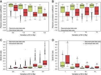
Either singletons are retained (Fig. 5, Supplementary Figs. S2, S3, Supplementary Tables S1–S3) or removed (Supplementary Figs. S4–S6, Supplementary Table S4–S6) from the discretized and thus reconstructed data sets, parameter D (mean biozone duration) appears to have the highest relative impact on the quality of the original discretized and original reconstructed curves as estimated by Pearson correlation. Clearly, the smaller D is (i.e., the shorter the mean biozone duration), the lower the absolute as well as relative amount of false co-occurrences generated by the time-discretization procedure, and the higher the overall correlations between the three taxonomic-richness curves (Fig. 5A), a result confirmed by multiple correlation analysis (Supplementary Table S1). Next, parameter M (mean taxon longevity) also appears to have a rather high impact on the diversity curve correlations, especially for the original–reconstructed curves correlation (Supplementary Table S1). For a larger M (i.e., a longer mean taxon longevity), the correlation is higher between the original and reconstructed time series (Fig. 5B). This result can be explained by the way the reconstructed signal is obtained from the discretized one: calculating new continuous-time origination and extinction ages necessarily modifies the original longevity of each taxon; the larger M is, the lower the average relative difference between original and reconstructed ages and thus longevities, the more parallel the original and reconstructed time series, and so the higher their correlation. Ultimately, this dependence on M exists because the mean biozone duration is noticeably shorter than the mean taxon longevity in 12/16 {M, D} simulated combinations, a situation also encountered in most real data sets due to the combinatorial nature of biozone construction. The N (number of simulated taxa; Supplementary Fig. S2A) and T (length of the simulated time interval; Supplementary Fig. S2B) parameters appear to have no major effect on the original–reconstructed curve correlation but more strongly affect the original–discretized curve correlation (see Supplementary Results).
Box plots showing the distributions of the Pearson correlation between the original and discretized (red) and the original and reconstructed (green) taxonomic-richness time series (including singletons) depending on the two main simulation parameters D (A), M (B), and box plots showing the distributions of the Qd ratio between the original and discretized (red) and Qr ratio between the original and reconstructed (green) taxonomic-richness time series (including singletons) depending on the two main simulation parameters D (C), M (D), and all {A, C} parameter combinations considered simultaneously. See Supplementary Fig. S2 for corresponding results without singletons.

Next, we looked at the Qd, Qr, and %UTB metrics as complementary estimates of the accuracy of discretized (Qd) and reconstructed (Qr; see Supplementary Results for %UTB) richness values with respect to the original ones. From the Qd and Qr perspective (Fig. 5, Supplementary Fig. S2, Supplementary Table S2), D and M appear to be the major control parameters: the smaller D is (mean biozone duration; Fig. 5C), or the larger M is (mean taxon longevity; Fig. 5D), the closer Qd and Qr are to 1, that is, the closer the discretized and reconstructed richness values are to the original ones. Again, these relations directly result from the false co-occurrences generated during the biozone construction (i.e., time-discretization) process: the larger D is and/or the smaller M is, the larger the number of false co-occurrences and the larger Qd and Qr, that is, the more the discretized and reconstructed richness values tend to overestimate the original signal. Comparatively, parameters N (number of simulated taxa; Supplementary Fig. S2C) and T (length of the simulated time interval; Supplementary Fig. S2D) have a weak average effect on Qd and almost no average effect on Qr values, even if the maximum simulated Qr and Qd values tend to increase with increasing N and T values. Overall, for any {D, M, N, T} combination, the reconstructed richness values appear much more accurate than the discretized ones (i.e., Qr is always closer to 1 than Qd).
Origination and Extinction Rates
Parallel to the sensitivity analysis of the taxonomic-richness signal, we also investigated the effects of varying T, N, M, and D (all {A, C} combinations considered simultaneously) on singleton-free Foote’s (Reference Foote2000) per capita-Myr origination
 $\left( {\hat{p}} \right)$
and extinction
 $\left( {\hat{q}} \right)$
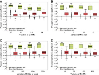
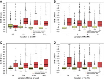
rates, using the same complementary metrics: Pearson correlation, Qd and Qr ratios, and %UTB. Whereas correlation levels reached by origination and extinction rates when comparing the original and reconstructed time series are globally similar (average correlations ranging from 0.7 to 0.9 in most cases), those obtained when comparing the original and discretized time series appear much lower (average correlations never larger than 0.3; compare Fig. 6 with Fig. 5 and Supplementary Figs. S2 and S4). Clearly, the discretized taxonomic rate time series fit the original one less well than its taxonomic-richness counterpart, a possible consequence of the nature of the taxonomic-richness dynamics as a combination of origination and extinction dynamics. Nevertheless, contrary to taxonomic richness–based results (see “Taxonomic Richness,” Supplementary Table S1), taxonomic rate–based multiple correlation analyses show somewhat different results depending on whether A=0 (no clustering of origination and extinction events around the biozone boundaries in the original data set; Supplementary Fig. S7; Supplementary Tables S7, S10) or A>0 (Supplementary Fig. S8; Supplementary Tables S7, S10). D (mean biozone duration) appears as the only leading control parameter when A=0, whereas both D and T (total length of the simulated interval) lead the original–discretized relation and N (number of simulated taxa) leads the original–reconstructed relation when A>0 (see Supplementary Results). From the Qd, Qr, and %UTB viewpoints, D, M and N appear to weakly affect both original–discretized and original–reconstructed time-series relationships, T playing a rather weak (%UTB) to no (Qd and Qr) role here (Fig. 7, Supplementary Fig. S9, Supplementary Tables S8, S9; see Supplementary Results). In all but one case (for D=0.5, i.e., very short mean biozone duration), the reconstructed origination and extinction rates values appear much more accurate than the discretized ones (i.e., Qr always closer to 1 than Qd).
Box plots showing the distributions of the Pearson correlation between the original and discretized (red) and original and reconstructed (green) time series of Foote’s (Reference Foote2000) taxonomic origination rate, depending on the four simulation parameters D (A), M (B), N (C), and T (D) and all {A, C} parameter combinations considered simultaneously. Similar results are obtained for extinction rates, as illustrated in Supplementary Table S10.

Box plots showing the distributions of the Qd ratio between the original and discretized (red) and Qr ratio between the original and reconstructed (green) time series of Foote’s (Reference Foote2000) taxonomic origination rate, depending on the four simulation parameters D (A), M (B), N (C), and T (D) and all {A, C} parameter combinations considered simultaneously. Similar results are obtained for extinction rates, as illustrated in Supplementary Table S11.

Robustness of the Reconstruction Algorithm to Varying Concentration of Originations and Extinctions around Biozone Boundaries
Building on the results presented above, we then investigated the effect of the clustering intensity of origination and extinction ages around biozone boundaries in the original (A) and reconstructed (C) data sets on the quality of the original–discretized and original–reconstructed time series of taxonomic richness and rates relations, as estimated by the same (Pearson, Qd, Qr, and %UTB) metrics. Here, results from 224 over the 256 possible {T, N, M, D} combinations are considered simultaneously. Simulation outputs when D=3.5 or 5.4 Myr and T=10 Myr (regardless of N and M values), corresponding to 2×16=32 distinct parameter combinations, were discarded to remove erratic results based on a biochronological framework involving very few (usually <5) successive biozones.
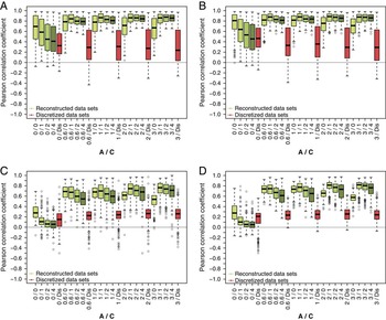
Based on the Pearson correlation related to the original–discretized and original–reconstructed curves relationships, the reconstructed signal appears to significantly outperform the discretized one in almost all {A, C} combination cases for both taxonomic-richness and rates time series (Fig. 8). This is most particularly true when A>0, whatever the value of C. Concerning taxonomic richness (either including or excluding singletons; Fig. 8A,B), average correlations range between 0.2 and 0.4 for the original–discretized relation, whereas they range between 0.4 and 0.8 when A=0 and between 0.65 and 0.9 when A>0 for the original–reconstructed relation. Concerning origination and extinction rates (Fig. 8C,D), average correlations range between 0.2 and 0.3 for the original–discretized relation, whereas they range between 0.05 and 0.3 when A=0 and between 0.6 and 0.8 when A>0 for the original–reconstructed relation. Therefore, from the Pearson correlation viewpoint, a taxonomic-richness or rate-discretized time series appears to poorly represent the original one, whereas its related reconstructed time series offers a much better fit, especially when A>0. That is, when origination and extinction ages are more or less concentrated around biozone boundaries in the original data set. Remarkably, even if the best correlation results are obtained for compatible A and C values, the reconstruction algorithm appears robust to discrepancy between these two parameters, especially when A>0. In that case, reliable reconstructed time series can be expected even if the actual value of A is ignored and even when C=0. Comparatively, when A=0, low average correlation values are expected even for the original–reconstructed relation, especially in the case of taxonomic rates, and all the more when C differs markedly from A. This suggests that, on average, discretized and reconstructed rates time series poorly fit the original rates time series when A=0, that is, as origination and extinction ages are randomly distributed within biozones.
Box plots showing the distributions of the Pearson correlation between the original and discretized (red) and original and reconstructed (green) time series of taxonomic richness including (A) and excluding (B) singletons, and Foote’s (Reference Foote2000) taxonomic origination (C) and extinction (D) rates, depending on the A and C simulation parameters (from lightest green for C=0 to darkest green for C=4), and all {T, N, M, D} parameter combinations considered simultaneously.

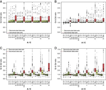
From the Qd and Qr viewpoints, the discretized time series appear to strongly overestimate the original taxonomic richness (with or without singletons) and the original taxonomic rates (median simulated Qd values significantly larger than 1), except for the case when A=0. It suggests the unbiasedness of Foote’s (Reference Foote2000) origination and extinction rates under a time-homogeneous rates evolutionary model (see “Simulation Results Based on Realistic {T, N, M, D} Parameter Combinations” for a more nuanced conclusion) (Fig. 9). However, the reconstructed taxonomic-richness time series still overestimate the original taxonomic-richness time series on average, but to a much lower extent, whereas simulation results appear more variable for reconstructed taxonomic-rates time series (see Supplementary Results).
Box plots showing the distributions of the Qd ratio between the original and discretized (red) and Qr ratio between the original and reconstructed (green) time series of taxonomic richness including (A) and excluding (B) singletons, and Foote’s (Reference Foote2000) taxonomic origination (C) and extinction (D) rates, depending on the A and C simulation parameters (from lightest green for C=0 to darkest green for C=4), and all {T, N, M, D} parameter combinations considered simultaneously.

Simulation Results Based on Realistic {T, N, M, D} Parameter Combinations
In a third and final step, we investigated simulation results based on four contrasted {T, N, M, D} parameter combinations inferred from the fossil record (Table 2). All but one (average taxonomic longevity for the Mesozoic radiolarian genera data set) parameter value used here fall within the ranges of parameter values used in the sensitivity and robustness analyses detailed above, making these last simulation results special realistic cases useful for illustration purposes.
From the taxonomic-richness viewpoint, Pearson correlation results highlight the importance of
 ${{\rm M} \over {\rm D}}$
, the ratio between the mean longevity of taxa (M) and the mean duration of biozones (D). The higher
 ${{\rm M} \over {\rm D}}$
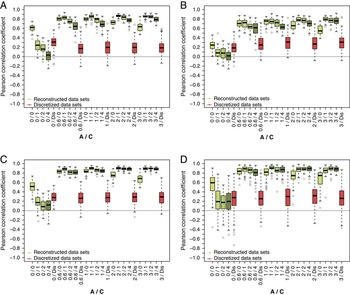
is, the higher the correlation between the original and discretized as well as reconstructed time series (Fig. 10: singletons included, Supplementary Fig. S11: singletons excluded). With
 ${{\rm M} \over {\rm D}}{\equals}\,9.5$
, the slowly evolving Mesozoic radiolarian genera parameter combination (Fig. 10A, Supplementary Fig. S11A) clearly returns higher correlation levels than the Meso-Cenozoic birds parameter combination (with
 ${{\rm M} \over {\rm D}}{\equals}1.4$
; Fig. 10B, Supplementary Fig. S11B), with the two mammal parameter combinations as intermediate cases (North American Cenozoic terrestrial mammals:
 ${{\rm M} \over {\rm D}}{\equals}\,3.8$
; Paleogene mammals from the Quercy and Limagne area:
 $${{\rm M} \over {\rm D}}{\equals}\,2.6$$
). In all cases, excluding singletons from the computations increases the correlations, all the more when originations and extinctions are not clustered around biozone boundaries (i.e., A=0) and when
 ${{\rm M} \over {\rm D}}$
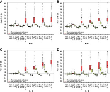
is large (compare Fig. 10A, Supplementary Fig. S11A with Fig. 10B, Supplementary Fig. S11B). Qd, Qr, and %UTB results highlight a similar effect of
 ${{\rm M} \over {\rm D}}$
on the accuracy of discretized and reconstructed taxonomic-richness values with respect to the original taxonomic-richness values (Fig. 11, Supplementary Fig. S12; see Supplementary Results). Overall, from the viewpoint of taxonomic-richness estimates and based on these four realistic parameter combinations (Table 2), the Mesozoic Radiolarian genera case demonstrates that a particular sets of parameters (e.g., with high
 ${{\rm M} \over {\rm D}}$
values) can greatly minimize the noise introduced during the discretization process, whereas other combinations (e.g., for Meso-Cenozoic bird genera) clearly illustrate the potentially large distortion effect of discretization. In all cases, the taxonomic-richness time series as reconstructed by the simple algorithm proposed here always exhibits a much better fit to the original time series than the discretized one.
Box plots showing the distributions of the Pearson correlation between the original and discretized (red) and original and reconstructed (green) taxonomic-richness time series (including singletons) for four distinct combinations of parameter values inferred from the fossil record (Table 2), depending on the A and C parameters (from lightest green for C=0 to darkest green for C=4). A, Mesozoic radiolarian genera. B, Mesozoic and Cenozoic birds. C, North American Cenozoic terrestrial mammals. D, Paleogene mammals from the Quercy area (France). See Supplementary Fig. S11 for corresponding results without singletons.

Box plots showing the distributions of the Qd ratio between the original and discretized (red) and Qr ratio between the original and reconstructed (green) taxonomic-richness time series (including singletons) for four distinct combinations of parameter values inferred from the fossil record (Table 2), depending on the A and C parameters (from lightest green for C=0 to darkest green for C=4). A, Mesozoic radiolarian genera. B, Mesozoic and Cenozoic birds. C, North American Cenozoic terrestrial mammals. D, Paleogene mammals from the Quercy area (France). See Supplementary Fig. S12 for corresponding results without singletons.

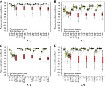
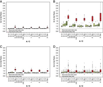
From the taxonomic rates viewpoint, Pearson correlation analyses for all four parameter combinations highlight the noisy effect of the discretization process on the original signal regardless of the value of A (i.e., the intensity of origination and extinction clustering around biozone boundaries), with average correlations between the original and discretized time series always ≤0.3 (Fig. 12, Supplementary Fig. S15). Departing from taxonomic-richness time series, this noisy effect also affects the original–reconstructed time-series relationship when originations and extinctions are not clustered around biozone boundaries (i.e., A=0) for all four {T, N, M, D} combinations. When A>0, the correlation between original and reconstructed taxonomic rates time series is clearly improved, but appears more strongly affected by A and C values than seen for the taxonomic-richness time series, with lower correlations for the most heterogeneous {A, C} combinations. Following the taxonomic-richness results detailed above (Fig. 10), the lowest average correlations are obtained from the Meso-Cenozoic bird genera parameter combination (Fig. 12B), especially for the original–reconstructed relationships. Overall, the main drivers of the correlation between the original, discretized, and reconstructed time series appears to be D and N: when A=0, small D values result in higher correlations, whereas higher N values generate higher correlations when A>0. Qd, Qr, and %UTB results highlight somewhat distinct situations, depending on A (Fig. 13, Supplementary Figs. S16–S18). Overall, based on Foote’s (Reference Foote2000) origination and extinction rates, an original data set resulting from a time-homogeneous rates evolutionary model (i.e., A=0) leads to unbiased to very weakly biased discretized and reconstructed taxonomic rates estimates, an appealing property that no longer applies when A>0, that is, under a time-heterogeneous rates evolutionary model.
Box plots showing the distributions of the Pearson correlation between the original and discretized (red) and original and reconstructed (green) time series of Foote’s (Reference Foote2000) taxonomic origination rate for four distinct combinations of parameter values inferred from the fossil record (Table 2), depending on the A and C parameters (from lightest green for C=0 to darkest green for C=4). A, Mesozoic radiolarian genera. B, Mesozoic and Cenozoic birds. C, North American Cenozoic terrestrial mammals. D, Paleogene mammals from the Quercy area (France). See Supplementary Fig. S15 for corresponding results for extinction rates.

Box plots showing the distributions of the Qd ratio between the original and discretized (red) and Qr ratio between the original and reconstructed (green) Foote’s (Reference Foote2000) taxonomic origination rate time series for four distinct combinations of parameter values inferred from the fossil record (Table 2), depending on the A and C parameters (from lightest green for C=0 to darkest green for C=4). A, Mesozoic radiolarian genera. B, Mesozoic and Cenozoic birds. C, North American Cenozoic terrestrial mammals. D, Paleogene mammals from the Quercy area (France). See Supplementary Fig. S16 for corresponding results for extinction rates.

Discussion
Based on the results presented above, two major discussion axes can be identified: (1) the effects of the transformation of an original, continuous-time diversity signal into a discrete-time signal and their consequences on the knowledge of deep-time biodiversity dynamics; and (2) the improvement in accuracy resulting from the back-transformation of a discrete-time taxonomic-richness data set into a virtually continuous-time data set. We discuss both aspects from the working hypothesis of a fully preserved and sampled taxonomic data set, that is, from the perspective of an exhaustively known complete fossil record including all taxa from the underlying living assemblages. We therefore deliberately ignore here all the methodological issues linked to the quality and reliability of paleontological data sets, including taphonomic biases (i.e., the degree to which a given fossil assemblage qualitatively and quantitatively actually reflects its parent living assemblage) and sampling biases (e.g., removing the rarest, smallest, or most fragile/fragmented specimens and species from the fossil record due to insufficient sampling effort or field, paleontological, or systematic expertise). In doing this, we obviously do not suggest that taphonomic and sampling biases have negligible or no effects on our knowledge of deep-time diversity dynamics; they do affect it. Rather, we ignore such biases by simulating complete fossil data sets with respect to their parent data sets to evaluate and discuss the still comparatively understudied effects of time discretization on our knowledge of deep-time biodiversity dynamics. This is the reason why we chose to use Foote’s (Reference Foote2000) taxonomic origination and extinction rates rather than Alroy’s (Reference Alroy2014, Reference Alroy2015) more recent rates integrating improved counting methods to minimize computational biases resulting from an incomplete fossil record. From that point of view, an exciting perspective deriving from the present study will be to add a taphonomic/sampling bias step to the simulation algorithm used here to further evaluate the relative accuracy and robustness of various diversity and rate metrics in paleontologically more realistic situations.
The qualitative and quantitative appraisal of biodiversity dynamics (considering either taxonomic richness, evolutionary rates, or any other metrics of interest) depends strongly on the spatial and temporal scale and resolution level at which data have been observed and recorded (Ricklefs Reference Ricklefs1987, Reference Ricklefs2004; Wiens Reference Wiens1989; Caley and Schluter Reference Caley and Schluter1997; Escarguel et al. Reference Escarguel, Fara, Brayard and Legendre2011). Even if the spatial scale of analysis is not explicitly taken into account in our simulation approach, it is implicitly accounted for, because the larger the geographical extent of the studied data set is, the larger N (a direct consequence of the species–area relationship; Rosenzweig Reference Rosenzweig1995) and D (for both ecological and biogeographical reasons, the absolute amount of biochronological contradictions between fossiliferous localities and sections is expected to increase with the geographical area under study, leading to a decrease in biochronological resolution and accuracy; Sadler and Cooper Reference Sadler and Cooper2008) are as well. In addition, T may also increase with the geographical extent of the study, but not M. From that point of view, by considering various contrasted {T, N, D} parameter combinations, our simulation approach actually covers a large spectrum of spatial and temporal resolutions from local (expected to imply relatively low T, N, and D values) to global-level analyses (expected to imply larger T, N, and D values). Alternatively, varying M and N (irrespective of T and D) indirectly accounts for varying the taxonomic resolution level of the analysis, from lower taxonomic-rank studies involving relatively small M values associated with large N/M ratios up to higher taxonomic-rank studies involving relatively large M values associated with small N/M ratios.
Finally, it is worth noting that all the simulations presented here were performed under a single, simple diversification scenario assuming stochastically constant diversity, origination, and extinction—a steady-state equilibrium (random walk) model ignoring the possibility of a nonrandom short-term event and/or a long-term background trend. Whereas nonrandom short-term changes in diversity are well known to paleontologists (e.g., extinction crises and adaptive radiation phases; Jablonski Reference Jablonski1986, Reference Jablonski2005; Hallam and Wignall Reference Hallam and Wignall1997), whether nonrandom long-term background trends in diversity changes actually existed or not over geologic times remains an open question falling largely beyond the scope of this work (Signor Reference Signor1978; Raup and Sepkoski Reference Raup and Sepkoski1984; Jablonski Reference Jablonski1986; Raup Reference Raup1991b; Alroy Reference Alroy1996, Reference Alroy2008, Reference Alroy2010b). Nevertheless, we note that the existence of such nonrandom events or trends may likely modify the relative impact of time discretization on the quality of the discretized and reconstructed diversity signals with respect to the original one. Actually, the steady-state diversification model used here is a worst-case scenario with respect to the original versus discretized versus average reconstructed time-series relationship—that is, the scenario that minimizes the diversity dynamics signal-to-noise ratio in the analyzed data set. Indeed, any nonrandom diversity event or trend added to this random walk process will necessarily increase the signal-to-noise ratio, ultimately improving the original versus discretized versus average reconstructed relationship. As a consequence, the back-transformation algorithm introduced here will generate at least equivalent if not better results when applied to nonstationary diversity patterns. From that point of view, a new key question arises: How much does diversity or rate need to deviate from background diversity dynamics to be able to detect the change with time-discretized data? Complementary simulations will be necessary to answer this question, building on the simulation algorithm used here by adding varying-intensity nonrandom events and/or trends in origination and/or extinction rates (and thus diversity). Critically, it will be necessary to distinguish among various cases, including origination and/or extinction short-term pulses versus long-term trends, with diversity-dependent or diversity-independent origination and/or extinction rates, which will severely increase the number of simulation outputs. This will also potentially affect the way the biozonation is constructed and applied to the original data set, as on average, shorter biozones are expected with increasing origination and/or extinction rates (Escarguel and Bucher Reference Escarguel and Bucher2004).
Effects and Consequences of the Discretization of a Continuous-Time Diversity Signal
The computation of correlation coefficient and Qd ratio related to the original–discretized time-series relationship for each of the 256 simulated combinations of {T, N, M, D} parameters and for four realistic parameter combinations: (1) provides an overview of the quality of the discretized diversity signal with respect to the original diversity signal; and (2) evidences the best and worst conditions to preserve the original diversity signal through time discretization, making it possible to estimate the potential overall effect of discretization on actual paleontological data sets, regardless of the additional effects of any taphonomic and/or sampling biases.
Original taxonomic-richness curves are best preserved through time discretization when mean biozone duration (D) is low and mean taxon longevity (M) is high, and thus when the
 ${{\rm M} \over {\rm D}}$
ratio is high (Fig. 5A,B, Supplementary Fig. S4A,B). The sensitivity analysis clearly illustrates the primacy of D over all other control parameters: the correlation coefficients computed between original and discretized taxonomic-richness time series when D=0.5 Myr are more than two times higher than when D=1.325 Myr, which in turn are nearly two times higher than when D=3.5 or 5.4 Myr. Beyond D, only M appears as an efficient control parameter. Indeed, realistic parameter combinations further show that even when a data set is built from a biozonation with a high D value (e.g., the Mesozoic Radiolarian genera data set; Table 2), the discretized richness curve remains close to the original one as long as M stays high, a situation classically encountered when studying long-ranging (slowly evolving or higher-level) taxa. While the
 ${{\rm M} \over {\rm D}}$
ratio plays a major role in controlling the quality of the relationship between the original and discretized taxonomic-richness time series, the total duration of the data set (T) and the number of simulated taxa (N) appear as second-order parameters, with higher correlation values when N is low and to a lesser extent when T is high, which indirectly increases the number of biozones over the simulated time interval, and thus decreases the relative importance of the false co-occurrence effect generated by time discretization (Supplementary Figs. S2C,D and S4C,D).
From the point of view of taxonomic origination and extinction rates, the relative effect of the control parameters on the correlation between the original and discretized time series is similar to those observed for taxonomic-richness curves up to when A=0, that is, the original, continuous-time origination and extinction ages for each taxon are not clustered around biozone boundaries (Supplementary Fig. S8, Supplementary Tables S4, S7). When A>0, that is, when origination and extinction ages are more or less strongly concentrated around biozone boundaries, the highest correlations between the original and discretized taxonomic rate curves are achieved by high N and D values combined with low T and M values (Fig. 7, Supplementary Tables S4, S7). This rather counterintuitive reversal of parameter influence with respect to the A=0 condition can be explained by the decrease of the relative amount of false co-occurrence generated by the time-discretization process (i.e., the decrease of average relative differences between original and discretized taxon longevity), as N and D increase and M decreases when the taxonomic turnover is concentrated around the biozone boundaries—an explanation supported by the fact that the higher A is, the more originations and extinctions cluster around biozone boundaries, and the greater the relative effect of D in controlling the quality of the original–discretized rates relationship. The fact that the main control parameters of the original–discretized rates relationship differ depending on whether A=0 or A>0 may be seen as problematic, because in most if not all real cases, the actual value of A is unknown. However, our simulation results clearly show that whatever A is, the correlation expected between the original and discretized taxonomic rate curves is very low (Fig. 6, Supplementary Figs. S7, S8), casting doubts on the overall accuracy of taxonomic rate relative changes through time based on even a complete paleontological data set.
Focusing on the Qd ratio, that is, exploring the degree to which the discretized rate time series consistently over- (Qd>1) or underestimates (Qd<1) the original rate time series, the mean biozone duration (D) only marginally affects the accuracy of the discrete-time rate estimates with respect to the original, continuous-time rate values, as expected for Foote’s (Reference Foote2000) origination and extinction rates (Fig. 9). However, Qd appears highly dependent on the value of A, the concentration level of originations and extinctions around biozone boundaries. When A=0, the discretized rate estimates are on average very close to the original ones, leading to Qd values close to 1, whereas when A>0, Qd consistently increases with A. The more originations and extinctions cluster around biozone boundaries, the more the discretized rates overestimate original rates, on average.
Overall, our simulation results lead to two contrasted conclusions. In most cases time variations of discretized time series of origination or extinction rates rather poorly correlate with original, continuous-time time series, indicating that the interpretation of relative changes in taxonomic rates may be strongly affected by the time-discretization process. However, discretized rates provide unbiased estimates of original rates on average when originations and extinctions are not more or less strongly clustered around biozone boundaries, that is, A ≅ 0. Even if the actual value of A is unknown for most if not all real paleontological data sets, we note that A ≅ 0 is expected when the biodiversity history of a given clade is investigated through a biozonation built on another, independently evolving clade with distinct life history traits. In that case, the origination and extinction dynamics of the clade under study are not expected to closely match the biozone boundaries, except when such limits coincide with global events having significant effects on biodiversity.
Back-Transformation of a Discretized Diversity Signal: Is It Worth Doing?
As discussed above, the discretization of an originally continuous-time biodiversity data set into a time-discontinuous data set through the construction of a biochronological framework is likely to lead to the loss of the absolute values and relative variations of the original signal. By assigning taxa to biozones, that is, by shifting origination ages downward and shifting extinction ages upward, time discretization modifies the distribution of taxonomic longevities and, most critically, generates false co-occurrences of taxa that actually did not coexist in time. This results in discretized time series potentially quite different from the original time series, depending on the {T, N, M, D, A, C} parameter combination. Recognizing such a major effect of time discretization on our knowledge of deep-time biodiversity history, the back-transformation of a discrete-time data set as customarily built from the fossil record by paleontologists and biostratigraphers into a virtually continuous-time averaged time series offers a straightforward solution. Interestingly, based on both Pearson correlation and Qd/Qr comparison metrics and whatever the original degree of origination and extinction clustering around biozone boundaries (controlled by parameter A), this solution appears robust and accurate from both taxonomic richness and origination and extinction rates points of view (Fig. 8). Nevertheless, the overall quality of the improvement resulting from this back-transformation algorithm depends on the combination of {T, N, M, D, A, C} parameter values. In the same way, the process of biozonation construction more strongly impacts the discretized origination and extinction rates curves than the discretized taxonomic-richness curves with respect to the original curves. As a consequence, the back-transformation algorithm leads to better results (i.e., higher improvement levels) for taxonomic richness than for origination and extinction rates.
From the point of view of taxonomic richness, best results based on the correlation between the original and reconstructed time series are obtained from short mean biozone durations (D), as illustrated by sensitivity analysis and simulations based on the realistic parameter combinations derived from the North American and French mammal data sets (Figs. 5, 10), both characterized by relatively low D values (1.325 and 0.95 Myr, respectively). Alternatively, from the point of view of the Qd and Qr ratios, best results are obtained from high values of mean taxon longevity (M), as also illustrated by sensitivity analysis and simulations based on the two other realistic combinations of parameters used in this work, both characterized by relatively large M values (7.4 and 26.7 Myr) (Figs. 5, 11).
The improvement generated by the back-transformation algorithm is lower for origination and extinction rates than for taxonomic richness, especially when A=0 (i.e., when originations and extinctions are not clustered around biozone boundaries). Nevertheless, the discretization effect on the original curves of origination and extinction rates is also the weakest when A=0. The worsening effect of discretization of an origination or extinction rate signal with respect to the original one increases with increasing A values, especially from the point of view of the Qd ratio. Overall, the improvement achieved by the back-transformation algorithm for origination and extinction rates is similar to that achieved for taxonomic richness when A ≠ 0 (Fig. 8). In that case, sensitivity analysis and simulations based on realistic parameter combinations show that a low D value (i.e., a short mean biozone duration) maximizes the improvement from the discretized to the reconstructed rate signal.
Interestingly, our results show that the level of improvement reached by the back-transformation algorithm does not critically depend on the value of C (Fig. 8), the concentration effect around biozone boundaries introduced in the back-transformation process. Best improvements are obviously achieved with A and C values leading to similar levels of origination and extinction clustering around biozone boundaries—the higher A is, the higher C is as well. However, high improvement levels are achieved with C=0 regardless of the actual value of A≠ 0, a noteworthy result, because A is unknown for most if not all real paleontological data sets. Conversely, when A=0, values of C larger than 0 generate rather poor results from both correlation and %UTB viewpoints. Therefore, whatever the real, but unknown value of A, use of a naïve C=0 value for the back-transformation algorithm appears as a rather robust and accurate solution that in most cases generates a reconstructed time series more closely agreeing with the original signal than the discretized one.
Conclusion
Regardless of the various taphonomic and sampling biases that inherently affect our knowledge of deep-time biodiversity history, the simulations presented in this work illustrate the usually strong deleterious effect of time discretization on an initially continuous-time signal, making time-discretized real paleontological data sets a possibly poor reflection of the genuine but unknown original biodiversity history. Indeed, even in an optimal context in which neither taphonomic nor sampling bias modifies the fossil record with respect to the original biodiversity history, time discretization through biochronological construction may dramatically affect the original versus discretized taxonomic richness and origination and extinction rate relationships by artifactually generating spurious coexistences of taxa within discrete time intervals (i.e., biozones). Ultimately, the sensitivity analysis performed based on 5120 distinct {T, N, M, D, A, C} control–parameter combinations shows that very weak to null correlations between original and discretized time series can be obtained from various realistic parameter combinations, a result further illustrated through additional simulations based on four contrasted {T, N, M, D} combinations taken from the fossil record (Table 2). Among the parameters controlling simulation results, the mean biozone duration (D) and taxon longevity (M) appear to be the main drivers of the quality of the original versus discretized time-series relationships, with best results (i.e., lowest deleterious effects) corresponding to high
 ${{\rm M} \over {\rm D}}$
values. Beyond these two main drivers, a low number of biozones (i.e., a low
 ${{\rm T} \over {\rm D}}$
value) and a high number of taxa (N) relative to the T, M, and D values are second-order but still efficient drivers of this negative effect.
Facing such effects of time discretization on the biodiversity signal, we introduce a simple and straightforward algorithm enabling the back-transformation into a virtually continuous-time averaged time series of a time-discretized data set as customarily constructed by paleontologists from the fossil record. By randomly generating new origination and extinction ages for each analyzed taxon within its respective origination and extinction biozones, this algorithm reduces the amount of spurious co-occurrences generated by time discretization, leading to reconstructed time series closer to the original signal than the discretized signals. We show that the level of improvement reached by this procedure is robust to the intensity of origination and extinction clustering around biozone boundaries, an interesting property when considering that the actual value of this parameter is unknown for most if not all paleontological data sets. Overall, we show that this procedure generates reconstructed time series closer to original time series than discretized ones for almost all simulated {T, N, M, D, A, C} parameter combinations, thus offering a significantly improved biodiversity signal even for parameter combinations adverse to an effective time-discretized reconstruction. The source code (written in R) of the back-transformation algorithm proposed and discussed in this work, which works for any real paleontological data set associated with a time-calibrated biozonation, is available in the Supplementary Material to this paper (http://dx.doi.org/10.5061/dryad.g9k46).
Acknowledgments
We thank Serge Legendre, Stéphane Dray, and Emmanuel Fara for stimulating comments and helpful advice; Maxime Gaudin for his help with C++ programming; and Matthew Makou for his helpful correction. We also thank Michael J. Foote and an anonymous reviewer for insights and comments that improved a first version of this article.
Supplementary Material
Data available from the Dryad Digital Repository: http://dx.doi.org/10.5061/dryad.g9k46