





1. Introduction
The Antarctic ice sheet (AIS) contains an estimated 58 m sea-level equivalent of ice (Morlighem and others, Reference Morlighem2020), making it Earth’s largest reservoir of ice and an important component in sea-level rise (SLR) projections. As the climate continues to warm, the AIS is losing mass at an accelerating pace (Pattyn and Morlighem, Reference Pattyn and Morlighem2020), which makes it increasingly critical to constrain its potential contribution to SLR. The mass loss primarily occurs through ice discharge from fast-flowing ice streams and outlet glaciers (Bamber and others, Reference Bamber, Vaughan and Joughin2000), and the rate and volume of ice being carried to the ocean are quantified by numerical models of glacier flow. Ice-stream velocity is strongly controlled by the bed (Alley and others, Reference Alley, Blankenship, Bentley and Rooney1986), and the numerical models must account for the processes of basal sliding and till deformation. However, the sliding process is poorly modeled because there remains a distinct lack of detailed information about the bottom of glaciers due to the difficulty of accessing and observing the glacier bed. This leads to large uncertainty in the ice-flow models and consequently SLR projections. There is therefore an urgent need to reduce this knowledge gap of the glacier bed.
Natural-source seismicity reveals important information about the glacier bed (Blankenship and others, Reference Blankenship, Anandakrishnan, Kempf and Bentley1987; Anandakrishnan and Bentley, Reference Anandakrishnan and Bentley1993; Anandakrishnan and others, Reference Anandakrishnan, Blankenship, Alley and Stoffa1998; Barcheck and others, Reference Barcheck, Schwartz and Tulaczyk2020; Kufner and others, Reference Kufner2021). As the glacier slides over its bed, friction between clasts in the ice and underlying bedrock (Zoet and others, Reference Zoet2013) induces small magnitude (local magnitude < 0) microseismic events known as icequakes, although larger-scale stick–slip events can produce higher magnitude icequakes (Zoet and others, Reference Zoet, Anandakrishnan, Alley, Nyblade and Wiens2012). In some cases, much of the basal shear stresses of ice streams is supported on ‘sticky spots’, localized regions of high basal drag surrounded by a weaker, low shear stress bed (Alley, Reference Alley1993; Anandakrishnan and Alley, Reference Anandakrishnan and Alley1994). These sticky spots are resolved seismically as discrete, highly repetitive spatial clusters of icequakes at the ice-stream bed (E. Smith and others, Reference Smith, Smith, White, Brisbourne and Pritchard2015; Hudson and others, Reference Hudson2023).
Here, we report observations of microseismicity, with a focus on icequake clusters and sticky spots, near the unexplored grounding line of Rutford Ice Stream (RIS) in West Antarctica. We use ‘grounding line’ to remain consistent with past literature and dataset naming conventions (Gudmundsson, Reference Gudmundsson2006; Hill and others, Reference Hill2023; Dinh and others, Reference Dinh, Rignot, Mazloff and Fenty2024), while recognizing that ‘grounding zone’ more accurately describes the spatially diffuse, tidally modulated transition from grounded to floating ice (Fricker and others, Reference Fricker, Coleman, Padman, Scambos, Bohlander and Brunt2009; Zhong and others, Reference Zhong, Simons, Minchew and Zhu2023; Rignot and others, Reference Rignot, Ciracì, Scheuchl, Tolpekin, Wollersheim and Dow2024).
2. Methods
2.1. Survey location and history
RIS is a major Antarctic ice stream flowing rapidly from the interior of the West Antarctic Ice Sheet (WAIS) in a south-southeast direction into the Filchner–Ronne Ice Shelf (Fig. 1a), draining an estimated 49 000 km2 of the WAIS (Doake and others, Reference Doake, Alley and Bindschadler2001). The RIS is situated in a deep trough bounded by the Ellsworth Mountains to the west and the Fletcher Promontory to the east (Fig. 1b). At RIS, several previous passive seismic surveys have focused on an inland study site approximately 40 km up-glacier from the grounding line. A pioneering study by A. Smith (Reference Smith2006) deployed ten geophones in a circular array with stations spaced 3 km apart, over 11 days. Further seismic studies at this site built upon the findings of that first study and improved network geometry, station density and deployment duration. These studies include E. Smith and others (Reference Smith, Smith, White, Brisbourne and Pritchard2015), which used a 10 station network in two subarrays with stations spaced 1 km apart, over 34 days, and Kufner and others (Reference Kufner2021), which used a larger 35 station rectangular network with stations spaced approximately 1 km apart, over 3 months. Ice-stream beds are composed of bedrock and unconsolidated sediment (till), and the inland study site lies at a boundary in bed character (E. Smith and others, Reference Smith, Smith, White, Brisbourne and Pritchard2015; King and others, Reference King, Pritchard and Smith2016; Kufner and others, Reference Kufner2021) which separates an up-glacier region of soft, deformable till from a down-glacier region of either stiffer till or weakly lithified sedimentary bedrock (A. Smith and Murray, Reference Smith and Murray2009; Schlegel, Reference Schlegel2022) with localized regions of soft till.
RIS grounding line study area. (a) Location of RIS in West Antarctica, which drains into the Ronne Ice Shelf. The map of Antarctica was obtained from the SCAR Antarctic Digital Database, showing seamask data (Gerrish, Reference Gerrish2024) and coastline data (Gerrish and others, Reference Gerrish, Ireland, Fretwell and Cooper2024). (b) Location of the 29 station grounding line array. RIS occupies a subglacial trough bounded by the Ellsworth Mountains to the west and Fletcher Promontory to the east, with ice flowing southeastward. The grounding line position is derived from Zhong and others (Reference Zhong, Simons, Minchew and Zhu2023). Map for panel (b) generated in ArcGIS Pro using the World Imagery basemap (Esri and others, Reference Esri2025).

Our study site is located just up-glacier of the RIS grounding line and, to our knowledge, is the first study to report seismic monitoring results near the RIS grounding line. Interferometric synthetic aperture radar (InSAR) surveys of RIS show that the ice surface velocities at the grounding line have fortnightly variations from approximately 0.9 to 1.2  ${\text{m da}}{{\text{y}}^{ - 1}}$, a variation of 27% of the total velocity, caused by tidal forcing dominated by the spring–neap tidal cycle (Gudmundsson, Reference Gudmundsson2006). The bed elevation at the grounding line is approximately 1500 m below sea level, with a complicated basal topography (Aðalgeirsdóttir and others, Reference Aðalgeirsdóttir2008). The grounding line lies down-glacier of the bed character boundary, and our study site overlies the stiffer bed domain where basal sliding is likely to dominate over till deformation (Stokes, Reference Stokes2018).
2.2. Data collection
We used 23 days of continuous passive seismic recordings (4–26 January 2019) to generate an icequake catalog near the grounding line of RIS, collected as part of the BEAMISH Project (A. Smith and others, Reference Smith2021). During the 2018/19 austral summer field season, we deployed 3 seismic arrays with a total of 59 seismometers around RIS that recorded seismic data ranging from December 2018 to February 2019. Two of the seismic arrays are approximately 40 km or more inland from the RIS grounding line and are outside the scope of this paper. We focus on the grounding line array (Fig. 1b), which consists of 29 stations (with station codes beginning with ‘166’) that started recording on 3 January 2019 and ended on 1 February 2019, with the exception of 2 stations (16653 and 16654) that ended recording earlier on 27 January 2019 and 31 January 2019, respectively.
Each station is a Magseis Fairfield Nodal system consisting of a 10 Hz three-component geophone with a 1000 Hz sampling rate, built-in data logger, batteries, solar panel and GPS antenna for synchronizing station times. Stations were buried 50 cm below the ice surface to improve coupling with the ice and reduce environmental noise. Previous icequake studies have emphasized the importance of dense, well-distributed networks and extended deployments for building comprehensive event catalogs that enable high-resolution characterization of icequake activity and support more robust analysis and interpretation (Aster and Winberry, Reference Aster and Winberry2017; Lombardi and others, Reference Lombardi, Gorodetskaya, Barruol and Camelbeeck2019; Hudson and others, Reference Hudson, Brisbourne, White, Kendall, Arthern and Smith2020a). Following these principles, our rectangular 29 station grounding line array employed 500 m interstation spacing over a 2.5 km × 2 km grid (5  ${\text{k}}{{\text{m}}^2}$ area), achieving a highly homogeneous network geometry. The higher station density increases the sensitivity of multiple stations to individual icequake events and improves isolation of the effects of spatiotemporal variations in basal properties on icequake activity. The month-long recording period provides a comprehensive view of persistent icequake activity.
Tidal height predictions near the RIS grounding line (A. Smith and K. Makinson, personal communication, 2020) include both diurnal (∼25 hours) and semidiurnal (∼12 hours) components. Temperature and atmospheric pressure loggers were installed on the ice shelf surface beyond the grounding line. Additional environmental data include qualitative weather logs from field notebooks with observational notes on meteorological (MET) conditions, useful for identifying events such as snowfall.
2.3. Data processing
To detect and locate icequakes and identify well-constrained clusters, we developed a three-step processing workflow. This workflow builds on the approach presented in Lee and others (Reference Lee, Anandakrishnan, Alley and Smith2026a)—detection and location with QuakeMigrate and clustering with Density-Based Spatial Clustering of Applications with Noise (DBSCAN)—excluding the GrowClust relocation step, and extends it with an additional clustering step using Hierarchical DBSCAN (HDBSCAN) to identify subclusters with varying densities. GrowClust was excluded because it did not meaningfully affect sticky spot structure and had limited impact on our analysis of relative event behavior within sticky spots. We provide a brief overview of each step here and refer to Lee and others (Reference Lee, Anandakrishnan, Alley and Smith2026a) for additional methodological details.
The workflow presented here was developed to optimize event identification and location, and to characterize seismicity on sticky spot asperities, while minimizing processing time and effort prior to scientific analysis.
2.3.1. QuakeMigrate
To detect and locate icequakes with the seismic data, we utilize QuakeMigrate (manuscript submitted to Seismica; preprint at EarthArXiv, doi: 10.31223/X53447; Bacon and others, Reference Bacon, Winder and Greenfield2023, Reference Bacon, Winder and Greenfield2025). QuakeMigrate is an open-source Python package for automatic earthquake detection and location using a waveform migration and stacking algorithm that searches for coherent seismic phase arrivals across a network or an array of instruments. The seismic waveforms are transformed into onset functions that describe the probability of phase arrivals, and continuously migrated and stacked in a subsurface search grid based on precomputed traveltime lookup tables (LUTs). QuakeMigrate computes the onset function using the short-term average to long-term average (STA/LTA) ratio of the signal energy amplitude. Coalescence, or coherent stacking, of onset functions that produces energy above a detection threshold indicates a potential icequake hypocenter (Winder and White, Reference Winder and White2020). QuakeMigrate is an ideal tool for detecting and locating icequakes at RIS because it coalesces signals from all stations within an array, amplifying the naturally weaker icequake signals for easier detection. From the raw seismic data, QuakeMigrate generates earthquake catalogs with event hypocenter locations, origin times, phase arrival picks, local magnitude (ML) estimates and rigorous estimates of the associated uncertainties.
We used a homogeneous ice velocity model with  ${V_p} = 3,841{\text{ m }}{{\text{s}}^{ - 1}}$ and
 ${V_s} = 1,970{\text{ m }}{{\text{s}}^{ - 1}}$ (
 ${V_{\text{p}}}$/
 ${V_{\text{s}}}$ ratio of 1.95) that matched observed RIS ice velocity values (A. Smith, Reference Smith1997; E. Smith and others, Reference Smith, Smith, White, Brisbourne and Pritchard2015; Kufner and others, Reference Kufner2021). Our QuakeMigrate grid extent was set to 10 km × 10 km, though we focused on the located basal seismicity in a 5 km × 4 km region within this grid in and around the RIS grounding line array. Table A1 in Appendix A lists the tuned QuakeMigrate parameter values for the RIS grounding line array, with brief notes where relevant.
2.3.2. DBSCAN
Prior studies have shown that icequakes in RIS occur in bursts of temporally and spatially focused activity (E. Smith and others, Reference Smith, Smith, White, Brisbourne and Pritchard2015; Kufner and others, Reference Kufner2021). We therefore searched for spatial patterns in our icequake catalog by grouping events that occurred close together. We used DBSCAN (Ester and others, Reference Ester, Kriegel, Sander and Xu1996), an unsupervised clustering algorithm, to identify these icequake clusters of concentrated activity. DBSCAN groups closely packed events based on a specified distance threshold and can capture varying cluster shapes while isolating noise. Because DBSCAN does not require a prespecified number of clusters, this flexibility supports our exploratory study of our icequake catalog.
Sticky spots are irregularly shaped patches, often approximated as circles for modeling purposes, which have been observed throughout Antarctica, ranging from about 10 m in diameter at RIS (Hudson and others, Reference Hudson2023) to more than 20 km in diameter at Whillans Ice Stream (Winberry and others, Reference Winberry, Anandakrishnan, Alley, Wiens and Pratt2014). Hudson and others (Reference Hudson2023) observed sticky spots at RIS with diameters on the order of 10–60 m. Based on these studies, we set an initial eps of 100 m—larger than the upper end of the expected sticky spot size range at RIS—to ensure that spatially coherent sticky spot events are grouped, with a conservative allowance for QuakeMigrate location uncertainty while still capturing the smallest sticky spots. This helps prevent over-segmentation and potential misclassification of genuine clusters as noise, which could obscure meaningful patterns in the data. We set min_samples to 2500 as a baseline for local event density—defined as the minimum number of events (including the event itself) required within a 100 m radius (i.e., the eps value) around an event for it to be considered dense enough to initiate or expand a cluster—reflecting the concentrated seismicity expected in coarse regions of sticky spots from which we aim to derive basal information.
Given the large number of events detected and located by QuakeMigrate, the initial application of DBSCAN with 100 m eps yielded spatially extensive clusters, as more loosely distributed events were grouped together. To further localize sticky spots, we iteratively reapplied DBSCAN within each cluster using progressively smaller eps values, grouping spatially concentrated events into well-constrained clusters (Fig. 2). Table A2 in Appendix A lists the tuned DBSCAN parameter values, with brief notes where relevant.
Method of iterative DBSCAN used to break down our RIS grounding line array catalog into well-constrained clusters. Arrows indicate the cyclical sequence of clustering and isolating. Step one shows clusters produced using an initial DBSCAN eps value of 100 m. In step two, we isolate one of these clusters—shown in green—for another DBSCAN iteration. Step three shows the resulting clusters using a smaller eps value. In step four, we isolate the blue cluster and again apply DBSCAN with an even smaller eps value in step five. The eps values used are guided by known sticky spot size ranges in RIS, the daily ice flow of 1 m  ${\text{da}}{{\text{y}}^{ - 1}}$ and QuakeMigrate location uncertainty. This process is repeated until clusters are well-constrained and also requires some familiarity with the expected spatial coherence of clustered events in RIS—in most cases, up to three DBSCAN iterations are sufficient.

2.3.3. HDBSCAN
With our DBSCAN cluster event locations, we conducted a more granular examination of the events within each cluster. We observed multiple distinct subclusters within the extent of the original cluster, which suggests a sticky spot smaller than initially clustered by DBSCAN, or potentially the presence of multiple smaller sticky spots in that cluster. As these subclusters have varied densities—indicated by differing average numbers of events per unit area—DBSCAN is not suitable for clustering them, since a fixed eps may overlook sparse but meaningful groupings or merge adjacent subclusters with differing density profiles. To identify subclusters with different densities, we employed the HDBSCAN algorithm (McInnes and others, Reference McInnes, Healy and Astels2017). Unlike standard DBSCAN, which uses a fixed spatial proximity threshold, HDBSCAN utilizes a tree-based hierarchy to discern clusters based on matching density environments. Since this density is based on the local relative density around each event, HDBSCAN is able to effectively capture clusters of varying densities. Figure 3 shows an example of HDBSCAN’s capability to detect and capture subclusters of varying densities and sizes. Table A2 in Appendix A lists the tuned HDBSCAN parameter values, with brief notes where relevant.
HDBSCAN subclusters of an example DBSCAN cluster from the RIS grounding line array. Thirteen subclusters are shown in color; the remaining white events are classified as noise. HDBSCAN’s ability to detect and capture clusters of varying densities produced a dominant central cluster (teal, n = 1240), along with other smaller clusters such as just up-glacier (blue) and three peripheral clusters (red, light blue and lavender) aligned transverse to the central cluster. Ice flow is from bottom left to top right.

3. Results
Running QuakeMigrate on the RIS grounding line array seismic data from 4 to 26 January 2019 yielded over one million located icequakes, averaging approximately 45 000 events per day within our search grid. We focused on events originating at or near the ice–bed interface, which are commonly associated with basal sliding. An example seismogram from a single station for a located basal icequake is shown in Fig. 4 for illustration. We removed events whose depth solution was significantly different than that of the bed (approximately 1650 m ice thickness), and events located more than several hundred meters beyond the array bounds, where location uncertainties increase. This filtering reduced the catalog from about one million events to 652 855 events. Event locations within the array were well constrained, based on the dense and uniform station geometry and the consistent concentration of basal events near the expected ice–bed interface—providing a robust basis for analyzing basal seismicity. In this section, we present the results, including event characterization, observations relevant to environmental factors and bed topography, and observations of repeating basal icequakes and sticky spots.
Example three-component seismogram of a located basal icequake from the RIS grounding line array at station 16613, showing the vertical (Z/GPZ) and horizontal (N/GP1 and E/GP2) components. Each trace spans a 1 s window and shows the phase arrivals (P- and S-waves) picked by QuakeMigrate. Amplitudes are in instrument counts and scaled to each trace’s minimum and maximum.

3.1. Event location uncertainty and validation
Our QuakeMigrate-located icequakes have a median location uncertainty of ∼200 m, while sticky spot events are better constrained at ∼125 m. These values represent absolute location uncertainties, whereas clustering is guided by spatial proximity and subsequently validated using waveform similarity and consistent relative arrival times. The strong similarity within sticky spot clusters indicates that their relative event locations are more tightly constrained than the absolute location uncertainties, such that spatial coherence among same-source events is preserved. Additional validation of QuakeMigrate event locations, comparisons with alternative event location methods and evaluation of relative relocation methods are presented in Lee (Reference Lee2026).
As the dominant frequency content of the icequake signals at the RIS grounding line is below 200 Hz, running QuakeMigrate at a 500 Hz sampling rate satisfies the Nyquist criterion (Havskov and Alguacil, Reference Havskov and Alguacil2016; Minowa and others, Reference Minowa, Podolskiy and Sugiyama2019) while improving computational efficiency and reducing runtime. Compared to the 1000 Hz runs, differences in event locations, MLs and picks for events detected in both the 500 and 1000 Hz runs were minimal and well within the combined propagated uncertainty bounds from both sampling rates.
3.2. Icequake focal mechanisms
To investigate the seismic source mechanisms that generated basal microseismic activity near our RIS grounding line array, fault plane solutions were determined from events using the first motion polarities of P-wave arrivals at each station, combined with S/P amplitude ratios, to characterize the focal mechanisms of the events. Icequake focal mechanisms were computed using the SKHASH software (Skoumal and others, Reference Skoumal, Hardebeck and Shearer2024). Broadly speaking, low-angle slip at the bed would result in the initial displacement to be compressional for stations down-slip (and in our case down-glacier), while stations up-glacier experience dilatation. This seismic radiation pattern (Aki and Richards, Reference Aki and Richards2002) has been observed in multiple glacier settings that trigger seismic activity (Walter and others, Reference Walter, Deichmann and Funk2008; Gräff and others, Reference Gräff, Köpfli, Lipovsky, Selvadurai, Farinotti and Walter2021; Stemland and others, Reference Stemland, Ruud and Johansen2023).
The mean slip vector from the SKHASH focal mechanism analysis, at 155.5°, closely matches the ice-flow direction of 148° measured at the inland site 40 km up-glacier from the grounding line (Kufner and others, Reference Kufner2023), indicating slip in the direction of flow. A mean dip of 9.3° (the ice is flowing slightly uphill) and a mean rake of 87.2° confirm the expected low-angle thrust faulting behavior typical of sticky spots, consistent with basal stick–slip sliding that generates repeating icequakes (Anandakrishnan and Alley, Reference Anandakrishnan and Alley1997; Anandakrishnan and others, Reference Anandakrishnan, Alley, Jacobel, Conway, Alley and Bindschadler2001; E. Smith and others, Reference Smith, Smith, White, Brisbourne and Pritchard2015). The focal mechanism of a sticky spot event is shown in Fig. 5. Similar patterns, including expected waveform polarities relative to fault geometry, were observed in other sticky spot events across the RIS grounding line array, further supporting this interpretation. These results align with focal mechanism observations at the inland site (E. Smith and others, Reference Smith, Smith, White, Brisbourne and Pritchard2015; Hudson and others, Reference Hudson, Brisbourne, Walter, Gräff, White and Smith2020b; Kufner and others, Reference Kufner2021).
Focal mechanism of an example sticky spot event (event time: 2019-01-12T10:03:39.584 UTC). (a) Lower hemisphere projection of the preferred focal mechanism (beachball plot) generated by SKHASH, with the shaded region indicating compression and the light regions indicating dilatation. P-wave first motion polarities (+ for compression and circle for dilatation, using SKHASH’s convention) and station positions are shown. The mean slip direction is 155.5° clockwise from true north at the top. The line through the beachball indicates the fault plane orientation. Station labels use the last two characters of the station (since all stations start with ‘166’) and are positioned at the four edges of the RIS grounding line array. (b) As in (a), but with the S/P amplitude ratios for each station shown, scaled by circle size. (c) Map view of the event location in the array network, with the same focal mechanism shown in (a) and (b). Ice-flow azimuth is 148°.

3.3. Gutenberg–Richter scaling of basal icequakes
The Gutenberg–Richter (G–R) relationship provides a widely used statistical framework for describing the magnitude-frequency distribution of earthquakes. In Eqn (1) (Gutenberg and Richter, Reference Gutenberg and Richter1944):
 \begin{equation}{\text{lo}}{{\text{g}}_{10}}\left( N \right){ } = { }a{ } - { }bM\end{equation}
N is the number of events with magnitude greater than or equal to magnitude M, a reflects the overall level of seismicity and b is the b-value, which characterizes the relative proportion of small to large events. ML estimates from QuakeMigrate were used to compute b-values after removing nonbasal events and events far from the array. We bin the 652 855 filtered events into bins of width 0.05 in magnitude; Fig. 6a shows the icequake ML distribution, with a magnitude of completeness (Mc; Wiemer and Wyss, Reference Wiemer and Wyss2000; Woessner and Wiemer, Reference Woessner and Wiemer2005) of −1.85. Mc provides an estimate of the lower bound above which QuakeMigrate reliably detects events. Figure 6b indicates the upper bound of the G–R relationship, where event frequency begins to plateau and deviate from the expected power-law trend (Pisarenko and Sornette, Reference Pisarenko and Sornette2004), at approximately −0.2. Taken together, the lower and upper bounds indicate the range over which the G–R analysis is considered robust, and allow for extrapolation to estimate the expected number of undetected smaller events at lower ML levels.
ML distribution of basal icequakes at the RIS grounding line array during the recording period (4–26 January 2019), shown in bins of 0.05. (a) Full ML distribution (excluding a small number of anomalous events) with a peak and Mc of −1.85. Events smaller than Mc (dashed bars) are excluded from the G–R analysis as they fall below the completeness threshold. The green region denotes the ML range used for G–R analysis. (b) Magnified view of the upper end of the green region in (a), highlighting the high-magnitude tail. The upper bound of −0.2 for the G–R analysis marks the point beyond which event frequency begins to plateau and deviate from the expected power-law trend.

The G–R relationship of the RIS grounding line array basal seismicity is shown in Fig. 7. We fit b-values to two separate magnitude ranges, as shown in Fig. 7b, following approaches used in icequake studies in RIS (E. Smith, Reference Smith2015; Kufner and others, Reference Kufner2021) and elsewhere in Antarctica (Huang and others, Reference Huang, Udell Lopez and Olsen2022). This gives a b-value of 2.17 for the smaller events from −1.85 to −0.4 ML, and a b-value of 5.50 for the larger events from −0.4 to −0.2 ML. Using a single-scaling regime yields a b-value of 2.37. Our b-values are substantially higher than those typically observed in tectonic settings and at larger magnitudes, where values are generally close to 1.0 (Frohlich and Davis, Reference Frohlich and Davis1993; Roux and others, Reference Roux, Marsan, Métaxian, O’brien and Moreau2008). High b-values are commonly associated with swarm-like seismicity, characterized by a relative excess of smaller events compared to larger ones (Horálek and others, Reference Horálek, Fischer, Einarsson, Jakobsdótir, Beer, Kougioumtzoglou, Patelli and Au2015), often linked to fluid intrusion or pressure-driven triggering mechanisms (Hainzl, Reference Hainzl2004; Aerts and Bilek, Reference Aerts and Bilek2025).
(a) Cumulative magnitude-frequency distribution of ML at the RIS grounding line array, shown in bins of 0.05, along with the curve of the local slope. Local slope refers to the derivative of log 10(N) at each magnitude bin. The gray vertical dashed line marks a sharp change in local slope around −0.4 ML. (b) G–R relationship of basal seismicity at the RIS grounding line array. The blue and red lines represent two separate b-values fitted to the magnitude ranges −1.85 to −0.4 ML (b = 2.17) and −0.4 to −0.2 ML (b = 5.50), respectively, defined by the slope break identified in (a). A single-scaling fit across the entire bounded magnitude range yields a b-value of 2.37 (purple line).

Our results are broadly consistent with findings from prior studies at RIS. Reported b-values (3.3 and 10.9 for Kufner and others, Reference Kufner2021; 1.8 and 15.9 for E. Smith, Reference Smith2015) differ from ours (2.17 and 5.50), particularly for the higher magnitude range; these differences may reflect the catalog sizes and the array geometries used. All three studies exhibit a similar pattern of two b-values across magnitude ranges, with higher b-values at the upper end.
3.4. Environmental factors and seismicity
Figure 8 shows the Pearson correlation coefficients (r) of tidal, surface temperature and atmospheric pressure time series with seismicity rate. The corresponding r values are 0.079 (Fig. 8a), 0.161 (Fig. 8b) and −0.271 (Fig. 8c).
Correlation of environmental data time series with seismicity rate, spanning the RIS grounding line array recording period from 4 to 26 January 2019. Seismicity rate is computed from event count, sampled at the same temporal resolution as each environmental variable: (a) tidal height predictions (1 hour interval),  $r = 0.079$; (b) surface temperature measured on the ice shelf (4 hour interval),
 $r = 0.161$; and (c) atmospheric pressure measured on the ice shelf, recorded by two surface-mounted sensors (5 min interval),
 $r = - 0.271$.

3.5. Bed topography and icequake occurrence
To characterize bed topography around our RIS grounding line array, we used bed elevation data from King (Reference King2009) and King and others (Reference King, Pritchard and Smith2016). Beneath and immediately adjacent to our array, bed elevation varies around 1650 ± 100 m (Fig. 9), consistent with estimates of approximately 1650 m near the grounding line (A. Smith and Doake, Reference Smith and Doake1994; Schmeltz and others, Reference Schmeltz, Rignot and MacAyeal2001; Jenkins and others, Reference Jenkins, Corr, Nicholls, Stewart and Doake2006). This topography aligns with previous observations that the bed beneath RIS has a W-shaped profile, with a central ridge or prominent knoll that is 100–200 m shallower than the adjacent troughs (Doake and others, Reference Doake, Frolich, Mantripp, Smith and Vaughan1987; A. Smith and Murray, Reference Smith and Murray2009). The array extends laterally from near the central ridge into the left-lateral (looking down-glacier) flanking trough.
Bed elevation map around the RIS grounding line array. The lower portion of the array lies on a central high ridge, while the upper portion is situated in an adjacent trough, with a bed elevation difference of approximately 200 m.

Event density contour map of icequakes from the RIS grounding line array recording period (4–26 January 2019), overlaid on residual bed elevation data around the array. Warmer colors in the event density contours indicate higher event densities, and cooler colors indicate lower event densities. Moats appear as local depressions up-glacier of bedrock highs (i.e., bumps), with their tails extending down-glacier as similar local low-elevation troughs along the flanks of these bumps. Seismicity is concentrated in and around moats up-glacier of bedrock highs, as well as in and around troughs that flank bedrock highs and are often bordered by steep changes in residual bed elevation.

To resolve local rather than regional topography, we computed residual elevations by subtracting the smoothed bed elevation from the observed bed elevation. We generated our smoothed bed elevation using a circular spatial smoothing filter with a 1 km radius to avoid directional bias. Given our focus on local bed variations—particularly relative lows—residual elevation maps are especially valuable. By removing the regional slope, residual elevations highlight subtle depressions such as troughs and moats, features which can influence basal seismicity by modulating subglacial water flow or local stress conditions. Figure 10 shows an event density contour map of icequakes from our recording period, after excluding nonbasal events and events distant from the array, overlain on the residual bed elevation.
Examples of repeating icequake event sets from the RIS grounding line array, where different sets exhibit different IEts, but each set has consistent IEts within its sequence. The repeating events are interspersed with other events, illustrating the need for careful location and analysis of waveform similarity, as described in the text. (a) Events repeating every 5 min. (b) Events repeating every 1.5 min (90 s). (c) Events repeating every 30 s; the dashed box encompasses both an upper panel showing events within the time series and lower panels displaying those same events individually, illustrating their waveform similarity.

In Fig. 10, we observed the highest icequake density over our 23 day recording period primarily in three main settings: (1) on the up-glacier sides of bumps—topographic highs that the ice is flowing against; (2) in moats—depressions eroded into the bed just up-glacier (i.e., on the stoss sides) of these bumps in response to flow diversion around the bedrock bumps; and (3) in the ‘tails’ of the moats—low-elevation troughs that are continuations of the moats—extending down-glacier parallel to ice flow and flanking ridges of mega-scale glacial lineations (MSGLs) or flutes composed of soft till deposited on the down-glacier (i.e., lee) sides of the bumps (A. Smith and others, Reference Smith2007; Alley and others, Reference Alley2021). A prominent moat lies near the center of the array, with a smaller one located just up-glacier. These moats and their tails mark the primary regions of seismicity, aligning in bands along ice flow. These seismic zones, particularly those around narrow troughs flanking bedrock highs and, in some cases, bounded on the opposite side by adjacent lows, often coincide with steep changes in residual bed elevation. The seismic activity occurs on stoss sides likely characterized by exposed bedrock or compacted tills, with or without a thin and perhaps discontinuous layer of soft till.
3.6. Repeating basal icequakes and sticky spots
The time between repeating events, defined as the interevent time (IEt), varies widely across glaciers. Prior work has reported relatively long IEts, from a mean IEt ≈ 12 hours for Whillans Ice Stream (Bindschadler and others, Reference Bindschadler, King, Alley, Anandakrishnan and Padman2003; Winberry and others, Reference Winberry, Anandakrishnan, Alley, Bindschadler and King2009, Reference Winberry, Anandakrishnan, Alley, Wiens and Pratt2014) to a mean IEt ≈ 25 min at David Glacier (Zoet and others, Reference Zoet, Anandakrishnan, Alley, Nyblade and Wiens2012). In both examples, longer IEts are associated with larger events because longer no-slip intervals allow the fault to recover strength and accumulate greater stress before failure (Abercrombie, Reference Abercrombie2021).
In contrast to the longer IEts observed at Whillans Ice Stream and David Glacier, events at our RIS grounding line array exhibit a variety of repeating signals with IEts of 5 min or less. Three examples of repeating events with different IEts are shown in Fig. 11. These shorter-interval events share key characteristics with their longer-interval counterparts, including relatively consistent IEts during sticky spot active phases, with modulation, and a positive IEt–event size correlation. We explore these patterns in detail in the next few sections, focusing on the repeating events associated with our HDBSCAN-resolved sticky spots.
3.6.1. Waveform similarity
If two events originate from the same sticky spot, we expect the observed waveforms and relative arrival times across stations to be similar, reflecting a similar source location and propagation path. To assess this, we designated a ‘master’ event for each sticky spot, typically one with consistently strong arrivals at all stations and reliable location properties, including being located at or near the bed and having low location uncertainty. We then compared the master event to other events in the same sticky spot and observed matching relative arrival times across stations, along with remarkably similar waveforms between events at each station. Figures in Appendix B show waveform comparisons between the master event and events from the central sticky spot in Fig. 3 (Figs. B1–B3), as well as between events from the sticky spot just up-glacier of the central sticky spot and their corresponding master event (Figs. B4–B6).
In addition to visual inspection, we quantified waveform similarity by computing the waveform cross-correlation values for events. Waveforms were extracted using QuakeMigrate’s pick times, with a window size appropriate for capturing the full P-wave arrival. For example, events in the central sticky spot have a high mean intracluster cross-correlation of ∼0.86, compared to a background level of ∼0.68 from cross-correlating nonclustered events (i.e., intercluster and noise events). Some clusters surrounding the central sticky spot also show intracluster cross-correlation values that are slightly above background but lower than those of the central sticky spot, likely due to smaller sample sizes and greater QuakeMigrate pick uncertainty. However, visual inspection and alignment of waveforms indicate that these surrounding clusters contain events with similar waveforms and consistent relative arrival times, pointing to a common source within each cluster, making them sticky spots as well, albeit shorter-lived. The relatively higher similarity of the central sticky spot events, evidenced by both quantitative cross-correlation and visual inspection, suggests that when stick–slip occurs over a longer and more stable period, this behavior produces more consistently similar waveforms. In contrast, clusters active for shorter periods produce less consistent waveforms and may lack sufficient persistence to be confidently identified as sticky spots.
3.6.2. Sticky spot behavior during active phases
Given the large number of identifiable sticky spots in our dataset, with many different IEts (Fig. 11) but often similar behaviors, we focus on three illustrative examples that capture key behaviors observed across multiple sticky spots and highlight multiple active phases of a sticky spot. The examples correspond to distinct active phases between 10 and 14 January 2019 of the blue sticky spot in Fig. 12, which corresponds to the central HDBSCAN subcluster in Fig. 3. Note that the sticky spots in Fig. 12 were resolved using data from the full recording period (4–26 January 2019), while in Fig. 3, they were resolved using data from only 12 January 2019.
Location of the example sticky spot (blue, n = 5731) subcluster. The other two subclusters were also identified by HDBSCAN after multiple iterations of DBSCAN, as described in Section 2.3.2.

The ML time series encompassing the three active phases for the example sticky spot is shown in Fig. 13a, with the phases spanning 10–11 January, 11–12 January and 13–14 January 2019. This sticky spot produced 5731 events over the full recording period of 4–26 January 2019, with the majority (>60%) occurring during these three active phases. The ML time series exhibits a rise-and-fall pattern that is positively correlated with IEt. Unlike the sticky spots on Whillans Ice Stream and David Glacier, the ML (and correspondingly IEt) time series for this sticky spot in our RIS grounding line array shows no significant correlation with tidal height predictions (which include both diurnal and semidiurnal components) (r = 0.036), and our dataset is too short to assess correlation with the fortnightly spring–neap tidal cycle. Other sticky spots in the RIS grounding line region are also unlikely to have any significant correlation with the diurnal and semidiurnal tides, as the duration of their rise-and-fall patterns during periods of activity varies and generally does not align with the tidal signal.
ML time series for the example sticky spot. (a) Time series encompassing three distinct active phases between 10 and 14 January 2019 (10–11 January, 11–12 January and 13–14 January), separated by vertical dashed lines. Phase boundaries are marked by quiescent periods (no detected events) or clear drops in event density, in both spacing and sustained rate. (b–d) Individual ML time series for each active phase (b: 10–11 January; c: 11–12 January; and d: 13–14 January), with events color-coded by IEt. Rise-and-fall patterns are visible across all phases, with IEts positively correlated with ML. Figure adapted from Lee and others (Reference Lee, Anandakrishnan and Alley2026b).

The IEt distributions of the three active phases of the sticky spot are shown in Fig. 14a–c. Each active phase contains over 1000 events and consistently has a mean and median around 44 s and a standard deviation of approximately 15 s. These similarities suggest the sticky spot is slipping in a consistent manner when active, with regular stress accumulation and release cycles producing repeatable event timing. The distributions for 10–11 January and 11–12 January share a similar shape, with a central peak around 40 s, while 13–14 January shows a different, bimodal shape with peaks around 30 and 45 s. Aside from a few large outliers, most of the IEts fall within the 0–80 s range across all three active phases. In practice, the IEt range is likely narrower, as values far from the peaks contribute relatively few events. The lower end of IEts (0–20 s) is sparsely populated, possibly reflecting a minimum period required for shear stress to rebuild and for frictional strength of the fault at the ice–bed interface to recover through healing (Im and others, Reference Im, Elsworth, Marone and Leeman2017) before the sticky spot can appreciably fail again and generate a detectable icequake.
IEt distributions and ML–IEt event density contour plots for the three active phases of the example sticky spot. (a–c) IEt distributions in 5 s bins with summary statistics. (d–f) ML–IEt event density contour plots, with smoothed event densities computed using a kernel density estimate (KDE); brighter regions indicate higher event densities. IEt values above the 90th percentile, along with their corresponding ML values, are excluded to reduce outlier influence. All three phases exhibit a clear positive ML–IEt trend consistent with stick–slip behavior. (a, d) 10–11 January, (b, e) 11–12 January and (c, f) 13–14 January. (d) and (e) each exhibit a single dominant density peak, while (f) exhibits two distinct density peaks, with the peak patterns consistent with the distributions in (a–c). Contour plot format after Zoet and others (Reference Zoet, Anandakrishnan, Alley, Nyblade and Wiens2012). Figure adapted from Lee (Reference Lee2026).

The individual ML time series for the three active phases of the sticky spot are shown in Fig. 13b–d, where isolating each phase highlights the rise-and-fall patterns more clearly. Longer IEts generally occur at the higher end of MLs, and shorter IEts at the lower end. IEts also vary systematically with ML, becoming intermediate as magnitudes transition between the extremes. This pattern is consistent with expectations from fault healing time. The greater IEt variations at higher MLs likely reflect natural variability and uncertainty. To visualize the relationship between ML and IEt, Fig. 14d–f show ML–IEt event density contour plots for the three active phases of the sticky spot. Each phase contains over 1000 events, and their plots exhibit a clear positive trend, with longer IEts generally associated with larger MLs. While the strength of these trends varies slightly between active phases and can differ within a phase depending on whether a rising, falling or mixed subset of the time series is considered, the overall positive trend remains consistent. These positive trends support stick–slip behavior, as opposed to flatter trends that would suggest stable sliding.
4. Discussion
4.1. Influence of environmental factors on seismicity
The very weak tidal correlation with seismicity (r = 0.079) arises primarily from the diurnal and semidiurnal cycles. Tidal modulation of seismicity—if present—likely would be more strongly associated with the spring–neap (∼15 day) cycle, which produces the largest velocity and thus stress variations at the ice–bed interface (Murray and others, Reference Murray, Smith, King and Weedon2007; Minchew and others, Reference Minchew, Simons, Riel and Milillo2017). We note that our dataset is too short to clearly resolve longer spring–neap variations in seismicity if they exist (Gudmundsson, Reference Gudmundsson2006; Rosier and others, Reference Rosier, Gudmundsson and Green2015; Minchew and others, Reference Minchew, Simons, Riel and Milillo2017; Robel and others, Reference Robel, Tsai, Minchew and Simons2017). Visual inspection of the data suggests that there is greater seismicity when ice-flow velocity is expected to be decreasing from this tidal influence (spring to neap) and less seismicity during the neap-to-spring transition. This pattern is more clearly visible in the first spring–neap shown in Fig. 8a, and only partially visible in the second. Kufner and others (Reference Kufner2021) report little influence of tidal forcing on basal icequakes, with only a possible gentle modulation of event magnitude, ∼40 km upstream of the grounding line. An early passive array deployed at the RIS grounding line in 1979–80 recorded tidal seismicity, with near-surface events tending to occur on the rising tide (possibly related to surface strand cracks opening) and basal events on the falling tide (potentially basal crevassing) (personal communication from A. Smith, 2020). Whether velocity, flexure or other processes are involved in tidal influence on seismicity and whether they act through stress build-up, normal pressure, water drainage or other paths require additional data and modeling.
The weak correlation between surface temperature and seismicity (r = 0.161) is likely influenced by sensor exposure to direct sunlight, resulting in readings as high as 20°C. In addition, temperature change is unlikely to affect basal processes in this environment lacking drainage of surface meltwater to the bed and thus lacks a clear physical mechanism to directly influence basal seismicity; it is shown only for completeness.
The correlation between atmospheric pressure and seismicity, although weak (r = −0.271), is of interest. As shown in Fig. 8c, seismicity is slightly higher in the earlier part of the record when air pressure is lower, and lower in the later part of the record when air pressure is higher. In addition, seismicity drops rapidly through the two pressure spikes near days 16.5 and 22. Atmospheric pressure changes could influence seismicity through several mechanisms, affecting normal stress on both sticky spots and the intervening water system, with potentially complex effects on lubrication and seismicity. We hypothesize that atmospheric pressure modulates normal stress on sticky spots, such that lower pressure reduces normal stress and promotes more frequent slip with smaller events, whereas higher pressure increases normal stress and suppresses slip and yields fewer but larger events. Mean event magnitudes are generally higher during the latter half of the record when air pressure is higher and event rates are reduced. This pattern is also evident during the intervals near days 16.5 and 22, where the most pronounced drops in event rate during pressure spikes coincide with elevated mean event magnitudes. Kavanaugh and others (Reference Kavanaugh, Moore, Dow and Sanders2010) observed that precipitation loading influenced seismic behavior at Storglaciären in Sweden, and Clarke (Reference Clarke2003) reported similar effects at Trapridge Glacier in Canada—supporting the idea that surface loading can affect basal conditions through added weight alone, without requiring direct drainage from the surface to the bed. Atmospheric pressure variations but not snowfall were significant during our deployment; MET weather logs indicated predominantly calm and clear conditions, with only occasional instances of light snowfall. The absolute pressure changes were about 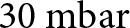 $30{\text{ mbar}}$—approximately 3% of standard atmospheric pressure (
 $1013.25{\text{ mbar}}$), or about 3 kPa. Note, though, that Tulaczyk and others (Reference Tulaczyk, Kamb and Engelhardt2001) suggested effective pressures beneath Whillans Ice Stream (Ice Stream B) of <20 kPa and likely 2 kPa, of the same order of magnitude as the atmospheric-pressure changes observed here. Further investigation is warranted.
4.2. Influence of bed topography on icequake occurrence
The observed relation between bed topography and basal seismicity suggests that local bed morphology influences where icequakes occur. Similar associations between bed topography and seismicity have been documented beneath Thwaites Glacier and farther inland on RIS, providing a framework for interpreting our observations.
At Thwaites, a combination of swath radar and seismic surveys across rugged subglacial highlands reveals strong spatial variability in bed properties—‘hard’ beds on stoss sides, with exposed ‘bedrock’ (poorly lithified sedimentary rock or possibly consolidated till), and ‘soft’ beds on lee sides, with porous, less consolidated till (Muto and others, Reference Muto, Alley, Parizek and Anandakrishnan2019a, Reference Muto2019b). In addition to stoss sides of topography, hard beds at Thwaites also occur in moats and their tails between soft-bedded flutes (Clyne and others, Reference Clyne, Anandakrishnan, Muto, Alley and Voigt2020; Alley and others, Reference Alley2021, Reference Alley2022). Previous studies and experiments indicate that glacier beds exhibit contrasting sliding behavior depending on substrate: more nearly viscous behavior on stoss sides where bedrock is exposed or till is consolidated, and more nearly plastic behavior on lee sides where deformation of soft, water-saturated till facilitates slip (Weertman, Reference Weertman1957; Kamb, Reference Kamb, Alley and Bindschadler2001; Koellner and others, Reference Koellner, Parizek, Alley, Muto and Holschuh2019; Zoet and Iverson, Reference Zoet and Iverson2020). Moats and their tails are interpreted as erosional features formed by ice flow around bedrock bumps, where basal shear stress is concentrated on stoss sides. These stresses promote bedrock erosion and till thinning on stoss sides, while lower effective pressure on lee sides allows transported till to be deposited and accumulate, forming flutes or MSGLs that produce the crag-and-tail features (Alley and others, Reference Alley2021). The harder bed regions promote stronger ice–bed coupling and elevated resistance to sliding, which enhances stress accumulation and favors stick–slip motion, increasing the likelihood of icequake nucleation. Similar bed properties are also likely beneath Whillans Ice Stream, where microseismicity has been observed in troughs (Barcheck and others, Reference Barcheck, Schwartz and Tulaczyk2020).
Extensive studies slightly farther up-glacier on RIS (King and others, Reference King, Woodward and Smith2007; A. Smith and others, Reference Smith2007; A. Smith and Murray, Reference Smith and Murray2009; E. Smith and others, Reference Smith, Smith, White, Brisbourne and Pritchard2015; Kufner and others, Reference Kufner2021) used passive and active seismic techniques colocated with high-resolution radar to provide further insights. Similar to Thwaites, an up-glacier region of relatively continuous soft bed, interpreted as deforming till, transitions down-glacier to bumps with stoss-side poorly consolidated bedrock and lee-side soft till-tail ridges or drumlins separated from adjacent soft ridges by harder-bedded troughs. Importantly, repeated surveying showed the deposition of a new drumlin (A. Smith and others, Reference Smith2007), demonstrating nonsteadiness in the system. The till flux from the deforming region up-glacier must be carried into and across the down-glacier region, possibly in spatially restricted areas, or nonsteadily, or as a deforming layer too thin to be resolved seismically. The seismicity on the harder regions is most easily explained as arising from debris-bearing ice moving directly over bedrock (e.g., Zoet and others, Reference Zoet2020), which favors the hypothesis of spatially or temporally restricted till transport or else strong entrainment of the debris transported from up-glacier into the ice. The rapid drumlin growth implies a large local convergence of sediment, consistent with both spatially and temporally restricted subglacial till transport, leaving regions of contact between debris-bearing ice and the local poorly lithified bedrock.
The structural similarity—hard beds on stoss sides and soft beds on lee sides—observed at both Thwaites and RIS, including near the grounding line and farther inland at RIS (King and others, Reference King, Woodward and Smith2007; Kufner and others, Reference Kufner2021), allows us to draw parallels and suggests that hard stoss-side beds in our study area promote stick–slip motion, contributing to the high density of icequakes observed in those regions. Figure 10 shows that icequakes are concentrated in and around moats located up-glacier of local bedrock highs (i.e., bumps), as well as in and around tails along the flanks of these bumps, where exposed or shallow bedrock is present. These bumps are sharper and more prominent in the up-glacier region, becoming broader and more subdued down-glacier. The up-glacier–down-glacier change in bump sharpness, with steeper up-glacier faces and gentler down-glacier flanks and lee surfaces, reflects erosion of resistant material on the up-glacier side and accumulation or smoothing by deformable till deposited on the down-glacier side. This seismicity pattern is consistent with regions of elevated basal resistance and with the findings of Kufner and others (Reference Kufner2021) at their inland array, approximately 40 km from the RIS grounding line, who found that seismicity was concentrated in the troughs between MSGLs and absent along their crests. They also observed that appreciable changes in residual bed elevation (e.g., 20 m) corresponded to greater seismicity, as such steps act as natural obstacles that concentrate stress and resist flow—a pattern we similarly observe in Fig. 10. In contrast, the soft, till-rich depositional zones that trail and extend directly down-glacier of these bumps contain few to no icequakes, consistent with lower resistance and weak ice–bed coupling in those regions.
Subglacial erosional features such as moats and troughs are generally thought to form either through meltwater flow (Dreimanis, Reference Dreimanis1993; Larter and others, Reference Larter2019) or, more likely, where drainage of abundant surface meltwater to the bed is absent, through enhanced coupling between ice and underlying sediment (Holschuh and others, Reference Holschuh, Christianson, Paden, Alley and Anandakrishnan2020; Alley and others, Reference Alley2021). A local example of the latter is an inland moat 22 km up-glacier from the RIS grounding line, reported by Schlegel and others (Reference Schlegel2024), who favor its formation by ice-driven erosion due to pressure against the rigid upstream end of an obstacle.
Together, these observations point toward a conceptual model in which sediment transport and episodic basal slip interact with underlying bed topography to shape seismicity patterns. During our 23 day study period, sticky spots were continuously active for brief periods of several days, during which they supported ice motion seismically and slipped total distances comparable to a significant portion of their fault patch extent. Such behavior may contribute to sediment reorganization and localized erosion, exposing bedrock and facilitating the development or maintenance of moats and troughs over longer timescales, while promoting till deposition directly down-glacier of the bumps. Future work using higher-resolution bed topography, such as that from swath radar, and longer seismic deployments would allow for finer-scale and more comprehensive resolution of this model, enabling more precise comparisons between icequake activity and basal features.
4.3. Sticky spot behavior
The three active phases of the sticky spot in Fig. 13 are separated by apparent quiescent periods with no detected events. These could reflect either stable sliding that generates no icequakes or tiny ‘baby’ events below our detection threshold. We suggest the latter is true because of the rise-and-fall patterns of adjacent active phases. The restart after a quiescent period is at an ML relatively similar to the ML just before that quiescent period. If stress had built up during quiescence (with no events at all), we would expect the events to resume at significantly higher MLs. This implies that even during apparent quiescence (i.e., below our detection threshold), icequakes may still be modulating stress. Though too small to reliably detect, these baby events likely preserve system memory, where each event retains and carries information from previous ones, producing systematic sequences of similar or incrementally varying magnitudes, mirrored by a strong positive IEt–ML correlation. A clear expression of this system memory is in the broader rise-and-fall pattern in Fig. 13a. The rise-and-fall patterns and their descents into the baby event regime will be explored further in a separate manuscript (Lee and others, in review, nonsteady basal hydrology). We note that a very careful effort to identify baby events from the same sticky spot was successful near the start and end of quiescent periods.
4.4. Sticky spot characteristics and slip behavior
Laboratory results (e.g., Zoet and others, Reference Zoet2020) and physical understanding indicate that the highly regular events such as those shown in Fig. 11 and observed on many of our active sticky spots arise from stick–slip motion accounting for all of the displacement, with stable sliding essentially zero. Here, we use simple seismic models to show that our data are consistent with this inference. Details of slip calculation, seismic moment estimation, source radius calculation and spectral fitting are provided in Appendix C.
For each active phase, we calculated event slips for all events using Eqns (C1–C3) and summed them to compare with the expected slip estimated from ice flow over that active phase period. Several assumptions underlie this calculation: (1) Each active phase window is defined based on where the event density is strong and sustained, with the bounds demarcated where it tapers off or becomes staggered, further informed by system memory based on the IEt. (2) We compare the total seismic slip during each active phase, measured from the first to the last event, to the total expected slip estimated from ice flow over the same time interval. (3) Events within each active phase have similar waveforms, a similarity generally confirmed through visual inspection. (4) The  ${\Omega _0}$–amplitude scale derived for this sticky spot holds for all its events, supported by consistent scaling across a wide range of amplitudes. (5) Only events clustered into the sticky spot by HDBSCAN are included in the calculation. A small but negligible number of events during the active phase were likely part of the sticky spot but were not clustered as such, contributing only very minor uncertainty to the total slip estimate.
In calculating seismic slip, four primary tunable source characteristics are considered: basal velocity  ${u_{\text{b}}}$, shear modulus μ, rupture velocity
 ${V_{\text{r}}}$ and corner frequency
 ${f_{\text{c}}}$. Each of these parameters can have a significant influence on slip estimates and is subject to varying levels of uncertainty.
For  ${u_{\text{b}}}$, while there are no direct basal velocity measurements on RIS, we estimated it based on measured surface velocities and prior estimates of basal-to-surface velocity ratios on RIS. The surface velocity at the RIS grounding line and our array is ∼1
 ${\text{m da}}{{\text{y}}^{ - 1}}$ (Doake and others, Reference Doake, Frolich, Mantripp, Smith and Vaughan1987; Sykes, Reference Sykes2009) and is modulated by tides up to 27% of the total velocity (Gudmundsson, Reference Gudmundsson2006), indicating dominant basal control, since tidal stresses act primarily at the bed. Analytical estimates further support basal sliding as the dominant component of flow on RIS (Frolich and others, Reference Frolich, Vaughan and Doake1989). The basal velocity is expected to be less than the surface velocity, but by how much remains uncertain. Frolich and Doake (Reference Frolich and Doake1988) estimated a difference on the order of 10
 ${\text{m }}{{\text{a}}^{ - 1}}$. Other prior models have taken basal velocity to be equal to surface velocity, on the assumption that internal deformation is generally small on RIS (Pralong and Gudmundsson, Reference Pralong and Gudmundsson2011). However, uncertainty remains high in partitioning basal sliding and internal deformation velocities due to the lack of direct measurements to distinguish their relative contributions to surface velocity at RIS, the possible role of ice anisotropy (Kufner and others, Reference Kufner2022) in softening the ice for deformation, and the potentially complex stress state near the grounding line, among other issues. We thus expect the basal velocity to be near but below the surface velocity ∼1
 ${\text{m da}}{{\text{y}}^{ - 1}}$. In the calculations below, we use 0.7 ± 0.15
 ${\text{m da}}{{\text{y}}^{ - 1}}$.
For μ, or rigidity, we used the shear modulus of the material where the majority of the elastic energy is stored, which, for debris-bearing ice moving over sedimentary bedrock, would be the μ of the bedrock (personal communication from C. Marone, 2024). While some elastic energy is likely stored in the basal ice, being near the pressure-melting point (Gudmundsson, Reference Gudmundsson2007) reduces its ability to sustain stress, so the majority of the elastic energy is stored in the bedrock. As described in Section 2.1, the bedrock at our RIS grounding line array is likely composed of stiff till or weakly lithified sedimentary bedrock, with the latter including materials such as sandstone or compressed sediment such as shale (Schlegel and others, Reference Schlegel2022). The μ for sandstone and shale varies widely and depends on several factors, including porosity, degree of lithification, clay content and saturation. Based on reported μ ranges for sandstone (∼1–30 GPa, Weijermars, Reference Weijermars1997; Avseth and others, Reference Avseth, Johansen, Bakhorji and Mustafa2014) and shale (∼0.2–14 GPa, tends to be softer than sandstone, Weijermars, Reference Weijermars1997; Asaka and others, Reference Asaka, Holt and Bakk2021), we adopt a RIS μ range of 3 ± 0.6 GPa (±20%). This value reflects a mix of shale, sandstone and possibly stiff till in a higher porosity, water-saturated region, which tends toward the lower end of the μ range, as the upper end reflects dry, well-lithified rocks. It falls within the typical range for weakly lithified sedimentary rocks and dense glacial till.
Computed seismic slip expressed as a percentage of the total expected slip estimated from ice flow during each of the three active phases of the sticky spot analyzed in this section.

Notes: The 10–11 January active phase spans 2019-01-10T16:00:00–2019-01-11T17:00:00 UTC, with a total duration of 25 hours. The 11–12 January active phase spans 2019-01-11T22:00:00–2019-01-12T19:00:00 UTC, with a total duration of 21 hours. The 13–14 January active phase spans 2019-01-13T07:00:00–2019-01-14T00:00:00 UTC, with a total duration of 17 hours (see Fig. 13 for the ML time series of these phases). The seismic and expected slips are calculated for the duration between the times of the first and last sticky spot event within each phase, which often differ slightly from the defined time ranges. The top data row shows seismic slip percentages using the nominal values of all four primary tunable source characteristics. The subsequent rows show the range of computed seismic slip percentages resulting from varying each characteristic individually within its uncertainty bounds while keeping the rest at their nominal values. The ranges of the source characteristics are:  ${u_{\text{b}}}$ (0.55–0.85
 $\rm{m}\,da{y^{ - 1}}$), μ (2.4–3.6 GPa),
 ${V_{\text{r}}}$ (1200–1600
 $\rm{m}\,{s^{ - 1}}$) and
 ${f_{\text{c}}}$ (125–145 Hz).
For  ${V_{\text{r}}}$, we estimated it as either a fraction of the S-wave velocity or the Rayleigh wave velocity. Rupture velocity is the speed at which the rupture front propagates along the fault and can be 50–90% of the shear wave velocity (Kaneko and Shearer, Reference Kaneko and Shearer2014). Our S-wave velocity at RIS is 1970
 ${\text{m }}{{\text{s}}^{ - 1}}$ (Kufner and others, Reference Kufner2021), from which we estimate a nominal
 ${V_r}$ of ∼1400
 ${\text{m }}{{\text{s}}^{ - 1}}$. Rayleigh wave velocities of ∼1600–1700
 ${\text{m }}{{\text{s}}^{ - 1}}$ measured at RIS (Zhou and others, Reference Zhou, Butcher, Brisbourne, Kufner, Kendall and Stork2022) and other glaciers (Mikesell and others, Reference Mikesell, Van Wijk, Haney, Bradford, Marshall and Harper2012; Walter and others, Reference Walter, Roux, Roeoesli, Lecointre, Kilb and Roux2015), derived from surface-sensitive methods that reflect near-surface structure (e.g., firn), provide an upper bound for glaciated settings. However, due to strong dependence on local firn structure and ice–bed properties, we use these values only to broadly constrain the upper end of the plausible range. These upper-bound values also reflect surface wave propagation, whereas our rupture velocity estimate applies to faulting at depth. Based on these values and the bimaterial nature of the fault (ice with clasts over stiff till or weakly lithified sedimentary bedrock, as described in Section 2.1), which suggests that
 ${V_{\text{r}}}$ falls between the Rayleigh wave velocities of the two materials (personal communication from C. Marone, 2025) and tends toward that of the weaker material (i.e., ice; Shlomai and Fineberg, Reference Shlomai and Fineberg2016), we adopt a RIS
 ${V_{\text{r}}}$ range of 1400 ± 200
 ${\text{m }}{{\text{s}}^{ - 1}}$.
For  ${f_{\text{c}}}$, direct observations from Brune fits to our spectral analysis (see Appendix C) of events from the three active phases of the sticky spot yielded a mean
 ${f_{\text{c}}}$ of approximately 135 Hz, with a relatively narrow range of ±10 Hz. We thus adopt a RIS
 ${f_{\text{c}}}$ range of 135 ± 10 Hz. This corresponds to an approximately ±10% variation, and using Eqn (C3) and the RIS
 ${V_{\text{r}}}$ range defined above, we obtained a sticky spot source radius range of ∼3–4.5 m. This represents the source radius of our example sticky spot; across the array, different sticky spots are expected to span a broader range of source radii. This radius lies at the lower end of sticky spot radii observed by Hudson and others (Reference Hudson2023) at RIS, which is reasonable given the tight spatial grouping and well-constrained event clusters resulting from our clustering methodology, as well as additional uncertainty beyond our assumed
 ${V_{\text{r}}}$ range, which could extend to higher values. The approximately ±10% range in
 ${f_{\text{c}}}$ leads to relatively small changes in source radius compared to the ∼1 unit change in ML observed across the ML ranges in Fig. 13, even though the ML of events used for the Brune fits span most of the overall range. While the source radii are expected to scale with event size as a power law (Hiramatsu and others, Reference Hiramatsu, Yamanaka, Tadokoro, Nishigami and Ohmi2002), the source radius remains relatively constant despite significant changes in event size. This decoupling between
 ${f_{\text{c}}}$ (and thus source radius) and event size may be due to other factors that modulate event size, such as hydrology or changes in normal stress, and will be explored further in a separate manuscript (Lee and others, in review, nonsteady basal hydrology).
Given the four primary tunable source characteristics and the significant influence each can have on computed seismic slip, we present a range of computed seismic slip estimates by varying each characteristic individually within its uncertainty bounds (here defined as plausible parameter ranges rather than formal statistical errors) while keeping the rest at their nominal values. Table 1 shows computed seismic slips, expressed as a percentage of the total expected slip estimated from ice flow during each active phase.
As shown in Table 1, using the nominal values (which yielded a sticky spot source radius of ∼3.6 m), our computed seismic slip closely matched the total expected slip, and this held consistently across all three active phases of the sticky spot. Varying each source characteristic individually produced significant changes in computed seismic slip percentage (i.e., computed seismic slip expressed as a percentage of the total expected slip), and tuning these characteristics simultaneously can, in practice, lead to even larger variations. Given these uncertainties, a seismic slip percentage of approximately 100 ± 50% during active phases is reasonable and remains within the same order of magnitude as the total expected slip. We thus infer that seismic stick–slip during active phases accounts for most or all of the total slip on the sticky spot. Since basal conditions such as driving and normal stress must change between stick–slip and stable sliding, it is unlikely that the system switches easily between the two. Thus, during active phases, the slip is most likely entirely seismic. We also observed that seismic slip is able to fully accommodate ice flow at other sticky spots within our RIS grounding line array during their active phases of varying duration. Shorter active phases showed greater variability in seismic slip percentages, with values less consistently close to 100%, likely due to smaller sample sizes and ramp-up effects during the transition from stable sliding to stick–slip. These results suggest that sticky spots across the RIS grounding line array enable stick–slip rather than stable sliding, and that their location distribution, as well as the timing and duration of their active phases, may provide insight into the relative contribution of stick–slip to overall ice motion at RIS. Furthermore, the range of tunable source characteristic values that yield physically reasonable results may provide insight into the mechanical properties and basal conditions of the RIS bed.
5. Conclusion
To investigate basal conditions at the RIS grounding line, we detected over one million icequakes from our array and identified sticky spots. Our workflow resolved well-constrained sticky spots with highly regular, repeating seismicity and similar waveforms. The basal icequakes were well-located and consistent with low-angle faulting in the ice-flow direction. Icequake magnitudes follow Gutenberg–Richter scaling consistent with swarm-like seismicity and exhibit two distinct b-values. We find that atmospheric pressure has a minor but non-negligible influence on seismicity at this array, suggesting external modulation of basal processes. Icequake density is higher in low-lying stoss-side moats and their down-glacier troughs, which contain hard beds that promote stick–slip motion. The example sticky spot analyzed in detail had an inferred source radius of ∼3.6 m. We show that seismic slip during active phases of sticky spots can fully accommodate ice flow, highlighting the role of stick–slip motion in RIS basal sliding dynamics.
Data availability statement
The raw seismic data are archived at the IRIS Data Management Center (IRIS DMC) under network code 5B (2018–19; https://ds.iris.edu/mda/5B/?starttime=2018-01-01T00:00:00&endtime=2019-12-31T23:59:59; Anandakrishnan, Reference Anandakrishnan2018). The Rutford grounding line array icequake catalog was generated using QuakeMigrate, with processing streamlined by the QuakeSupport package (Lee and others, Reference Lee, Anandakrishnan and Alley2025a), as described in Lee and others (Reference Lee, Anandakrishnan, Alley and Smith2026a). The catalog is accessible through the U.S. Antarctic Program Data Center (USAP-DC) at https://www.usap-dc.org/view/dataset/601932 (Lee and others, Reference Lee, Alley and Anandakrishnan2025b). The QuakeSupport repository is available at https://github.com/cryoilrj/QuakeSupport and is archived at https://doi.org/10.5281/zenodo.15460028. Both the catalog and QuakeSupport are freely available for public use and reuse in future research.
Acknowledgements
We thank the developers of QuakeMigrate (notably Conor Bacon, Tom Winder and Tom Hudson), whose tool played an integral role in our data processing and who were willing to address questions related to their software. We thank Luke Zoet, Chris Marone and Nate Stevens for answering questions related to slip computations and their underlying components. We thank members of the British Antarctic Survey (BAS) field team Andy Smith, Alex Brisbourne, Catrin Thomas and Rebecca Schlegel for field logistical support, and thank Alex Brisbourne, Catrin Thomas and Rebecca Schlegel for installing the array used in this study. We thank the staff at Rothera Research Station and BAS logistics for enabling the fieldwork associated with this project and the BEAMISH field team (2018/19) for acquiring the passive seismic data. Seismic instruments were provided by NERC SEIS-UK (Loan 1017), by BAS, and by the Incorporated Research Institutions for Seismology (IRIS) through the PASSCAL Instrument Center at New Mexico Tech. The facilities of the IRIS Consortium are supported by the U.S. National Science Foundation (NSF)’s Seismological Facilities for the Advancement of Geoscience (SAGE) Award under Cooperative Support Agreement EAR-1851048. This work was funded by NERC AFI award numbers NE/G014159/1 and NE/G013187/1, NSF awards 1643961 and 1738934 and the Heising-Simons Foundation. We thank the anonymous reviewers and Associate Chief Editor Chris Stokes for their constructive comments and suggestions, which improved the manuscript.
Author contributions
IL processed and analyzed the icequake data and wrote the manuscript. SA and RA provided scientific guidance and reviewed the manuscript. AS and AB provided scientific guidance and provided unpublished environmental (tidal, temperature, pressure) data discussed in this paper. CB and SKK provided IL with guidance on learning and tuning QuakeMigrate. AW assisted IL with processing the icequake focal mechanisms.
Appendix A: Parameters for icequake catalog generation and sticky spot resolution
QuakeMigrate parameters used for the RIS grounding line array.

DBSCAN and HDBSCAN parameters used for the RIS grounding line array primary analysis.

Appendix B: Waveform comparisons between sticky spot events
To illustrate similar waveforms and relative arrival times within sticky spots, we show three sample comparisons (Figs. B1–B3) between the master event and other events from the central sticky spot in Fig. 3. We also show three additional sample comparisons (Figs. B4–B6) between its corresponding master event and other events from the blue sticky spot just up-glacier of the central sticky spot.
P-wave arrival waveform comparison of two icequake events from the central sticky spot in Figure 3. The master event (blue; event time: 2019-01-12T01:26:39.975 UTC) is overlain by a comparison event (orange; event time: 2019-01-12T01:28:09.276 UTC) uniformly time-shifted to align arrivals. Waveforms from both events are highly similar at each station, in both shape and relative arrival time. (a) 500 ms window showing original relative timing preserved across all RIS grounding line array stations, capturing the full range from earliest to latest arrivals. (b) 80 ms window with arrivals centered in each time series.

P-wave arrival waveform comparison of the master event (blue; event time: 2019-01-12T01:26:39.975 UTC) overlain by a comparison event (orange; event time: 2019-01-12T00:06:27.829 UTC). Waveforms are uniformly time-shifted to align arrivals. (a) 500 ms window across all RIS grounding line array stations with preserved relative timing. (b) 80 ms window with arrivals centered.

P-wave arrival waveform comparison of the master event (blue; event time: 2019-01-12T01:26:39.975 UTC) overlain by a comparison event (orange; event time: 2019-01-12T18:40:49.551 UTC). Waveforms are uniformly time-shifted to align arrivals. (a) 500 ms window across all RIS grounding line array stations with preserved relative timing. (b) 80 ms window with arrivals centered.

P-wave arrival waveform comparison of master event (blue; event time: 2019-01-12T15:30:26.645 UTC) overlain by a comparison event (orange; event time: 2019-01-12T06:56:06.514 UTC). Waveforms are uniformly time-shifted to align arrivals. (a) 500 ms window across all RIS grounding line array stations with preserved relative timing. (b) 80 ms window with arrivals centered. Note that the centered arrivals are based on QuakeMigrate’s picks, which may incorrectly pick a stronger nearby signal when the true arrival is weak, as seen on several stations for this comparison event; hence, panel (a), which preserves relative timing across stations, provides a more reliable basis for comparison.

P-wave arrival waveform comparison of master event (blue; event time: 2019-01-12T15:30:26.645 UTC) overlain by a comparison event (orange; event time: 2019-01-12T15:35:02.304 UTC). Waveforms are uniformly time-shifted to align arrivals. (a) 500 ms window across all RIS grounding line array stations with preserved relative timing. (b) 80 ms window with arrivals centered. Note that the centered arrivals are based on QuakeMigrate’s picks, which may incorrectly pick a stronger nearby signal when the true arrival is weak, as seen on several stations for this comparison event; hence, panel (a), which preserves relative timing across stations, provides a more reliable basis for comparison.

P-wave arrival waveform comparison of master event (blue; event time: 2019-01-12T15:30:26.645 UTC) overlain by a comparison event (orange; event time: 2019-01-12T15:54:54.330 UTC). Waveforms are uniformly time-shifted to align arrivals. (a) 500 ms window across all RIS grounding line array stations with preserved relative timing. (b) 80 ms window with arrivals centered. Note that the centered arrivals are based on QuakeMigrate’s picks, which may incorrectly pick a stronger nearby signal when the true arrival is weak, as seen on several stations for this comparison event; hence, panel (a), which preserves relative timing across stations, provides a more reliable basis for comparison.

Appendix C: Seismic slip calculation, seismic moment estimation, source radius calculation and spectral fitting
We calculate the total seismic slip during each of the three active phases of the example sticky spot analyzed in Section 3.6.2 by computing the slip of each event from its seismic moment and summing over the corresponding phase. The slip of an event can be estimated from the equation:
 \begin{equation}D = \frac{{{M_0}}}{{\mu \cdot A}}\end{equation}
where D is the average slip over the rupture area A,  ${M_0}$ is the seismic moment and μ is the shear modulus of the underlying bedrock. The seismic moment
 ${M_0}$ is a measure of earthquake energy and is derived from the far-field P-wave displacement spectrum using the Fourier transform of eqn 4.88 in Aki and Richards (Reference Aki and Richards1980), as applied in Anandakrishnan and Bentley (Reference Anandakrishnan and Bentley1993) and Patton and Randall (Reference Patton and Randall2002):
 \begin{equation}{M_0} = \left( {\frac{{{\Omega _0} \cdot l}}{{{F^{\text{p}}}}}} \right)4\pi \rho _{\text{s}}^{\frac{1}{2}}\rho _{\text{d}}^{\frac{1}{2}}v_{{\text{ps}}}^{\frac{5}{2}}v_{{\text{pd}}}^{\frac{1}{2}}\end{equation}
where  ${\Omega _0}$ is the low-frequency spectral level,
 $l$ is the source-receiver distance,
 ${F^{\text{p}}}$ is radiation-pattern correction,
 ${\rho _{\text{s}}}$ and
 ${v_{{\text{ps}}}}$ are the density and P-wave velocity at the source and
 ${\rho _{\text{d}}}$ and
 ${v_{{\text{pd}}}}$ are the density and P-wave velocity at the detector (i.e., the station). We used a standard
 ${F^{\text{p}}}$ of 0.5 to approximate the average effect of source-receiver geometry (Boore and Boatwright, Reference Boore and Boatwright1984). l from the sticky spot to the nearest down-glacier station is ∼1716 m.
 ${\rho _s} = 1087{\text{ kg }}{{\text{m}}^{ - 3}}$ and
 ${\rho _d} = 917\,{\text{kg }}{{\text{m}}^{ - 3}}$;
 ${v_{ps}} = 3841\,{\text{m }}{{\text{s}}^{ - 1}}$ and
 ${v_{pd}} = 3800\,{\text{m }}{{\text{s}}^{ - 1}}$. The higher source density and P-wave velocity, relative to those at the detector, reflect ice with higher debris content and possible influence from the underlying bedrock, in contrast to the cleaner glacial ice near the surface at the detector (personal communication from L. Zoet, 2023).
The sticky spot rupture area is approximated as a circle with area  $\pi {r^2}$, where r is the source radius. We calculate r using the equation derived from the circular crack model of Brune (Reference Brune1970):
 \begin{equation}r = \frac{{1.1 \cdot {V_{\text{r}}}}}{{\pi \cdot {f_{\text{c}}}}}\end{equation}
The constant factor 1.1 is included as an empirical adjustment that accounts for finite rupture velocity and the use of P-wave corner frequencies (Madariaga, Reference Madariaga1976; Orefice, Reference Orefice2012). Here,  ${V_{\text{r}}}$ is the rupture velocity and
 ${f_{\text{c}}}$ is the P-wave corner frequency. Note that the Brune model assumes a circular rupture patch (Brune, Reference Brune1970), whereas the actual sticky spot is likely to be irregularly shaped with rough or diffuse boundaries, introducing additional uncertainty.
To estimate the corner frequency  ${f_{\text{c}}}$ and low-frequency spectral level
 ${\Omega _0}$ of an event, we computed the Fourier transform of the P-wave arrival to obtain the displacement amplitude spectrum. As our slip is an estimate, we used data from the nearest down-glacier station for each event, which likely receives the strongest signal, and did not account for attenuation or source-receiver distance variations in corner frequency. The P-wave window used for the transform was derived from QuakeMigrate’s pick time, with the window positioned around the phase arrival to capture the full signal while minimizing contamination from other events or later phases. P-waves are used because they arrive first and are less affected by scattering, allowing cleaner estimates of source parameters from the displacement amplitude spectrum. We removed the instrument response from our raw seismic data, recorded in instrument counts, along with integration to displacement, and the resulting displacement signals were bandpass filtered between 10 and 450 Hz to isolate the frequency range of interest, avoiding both low instrument sensitivity below 10 Hz and the Nyquist frequency at 500 Hz (for a 1000 Hz sampling rate). We also corrected for a 24 dB field gain that was applied during the field season. We then computed the displacement amplitude spectrum by first subtracting the mean (DC offset) from each trace, applying a Hann window to reduce spectral leakage, and performing a one-sided fast Fourier transform (FFT). The resulting spectrum was normalized to account for windowing energy loss and ensure accurate amplitude scaling. Following Brune (Reference Brune1970), we fit the displacement amplitude spectrum using a source spectral model to estimate the
 ${f_{\text{c}}}$ and
 ${\Omega _0}$:
 \begin{equation}\Omega \left( f \right) = \frac{{{\Omega _0}}}{{1 + {{\left( {\frac{f}{{{f_{\text{c}}}}}} \right)}^2}}}\end{equation}
where  $\Omega \left( f \right)$ is the displacement amplitude spectrum at frequency f. We exclude unreliable values by filtering out zero, nonfinite and sub-10 Hz amplitudes to avoid noise contamination and issues with logarithmic scaling. The Brune model is then fit using nonlinear least squares, with initial guesses based on the peak spectral amplitude and its corresponding frequency. A sample event from the sticky spot, with its P-wave arrival and corresponding displacement amplitude spectrum fitted to the Brune model, is shown in Fig. C1.
In Fig. C1,  ${\Omega _0}$ corresponds to the flat spectral plateau before
 ${f_{\text{c}}}$. Frequencies below 10 Hz were excluded from the Brune fit due to reduced instrumental sensitivity, and
 ${\Omega _0}$ was determined from the sustained flat plateau of the spectrum.
 ${f_{\text{c}}}$ marks the transition from this low-frequency plateau to a consistent high-frequency decay. A double dip appears at high frequencies: the initial break in slope marks the corner frequency (
 ${f_{\text{c}}}$ = 137 Hz), where the spectrum begins to decay, while the second, deeper dip (around 300 Hz) is not physically meaningful and likely due to nonlinearities in the geophone response at high frequencies (King and Bell, Reference King and Bell1996). Minor ripples between the dips are consistent with spectral processing artifacts and are not source-related features. Accordingly, we interpret the second dip as a notch within the same high-frequency falloff, not a source process. The steepness of the spectral decay is primarily due to the strong high-frequency seismic attenuation in ice, which has a lower quality factor (Q) than rock (Peters and others, Reference Peters, Anandakrishnan, Alley and Voigt2012). Additional steepening may also result from nonlinearity in the geophone response, bandpass edge effects or spectral interference. These effects produce steep high-frequency decay and ripples that the Brune model, which assumes smooth spectral falloff, does not reproduce well. Fits thus tend to be less robust for smaller-magnitude events, and in such cases, visual inspection is often the most reliable method to verify
 ${f_{\text{c}}}$.
We applied the Brune model fit to selected events across the three active phases of the sticky spot. Since these events originate from a common source, we expected them to have similar waveforms and  ${f_{\text{c}}}$, and thus comparable source radii. To assess whether a consistent
 ${\Omega _0}$–amplitude relationship could be applied across events, we plotted
 ${\Omega _0}$ values against P-wave peak amplitudes from the nearest down-glacier station, noting that
 ${\Omega _0}$ is proportional to seismic moment, which scales with event size (Brune, Reference Brune1970), while peak amplitude provides a relative measure of event size at a common station for events from the same source. Figure C2 shows an illustrative
 ${\Omega _0}$–amplitude plot for the sticky spot. The result was a well-defined linear relationship, and the fit remained robust despite some events containing arrivals from other events or noise within their processing window, indicating that the scaling is stable. The
 ${\Omega _0}$–amplitude relationship was established using events spanning multiple active phases and the observed range of amplitudes. The linear
 ${\Omega _0}$–amplitude scale allows estimation of
 ${\Omega _0}$ for each event in the sticky spot, allowing us to quickly estimate
 ${\Omega _0}$ for all events without the need to fit the Brune model to spectra for each one. Similar linear scales can be established separately for individual sticky spots.
Sample event (event time: 2019-01-12T04:23:30.994 UTC) from the sticky spot showing the P-wave arrival and corresponding displacement amplitude spectrum. (a) P-wave arrival on the vertical GPZ component recorded at the nearest down-glacier station 16613 within a 200 ms window, amplitudes in instrument counts. (b) Displacement amplitude spectrum on a log-log scale, fitted to the Brune model  $\Omega \left( f \right)$ defined in Eqn (C4). The orange vertical dashed line marks the corner frequency
 ${f_c} = 137$ Hz, where the spectrum begins to decay. The low-frequency spectral level
 ${\Omega _0} = 2.598 \times {10^{ - 11}}$ m·s corresponds to the flat portion before
 ${f_{\text{c}}}$. Although the y-axis is labeled in [m] by convention,
 ${\Omega _0}$ has units of m·s due to the Fourier transform.

Plot of  ${\Omega _0}$ versus P-wave peak amplitude from the nearest down-glacier station for events from the sticky spot. Events selected from across the three active phases of the sticky spot and spanning the observed range of amplitudes are shown as pink circles. A least-squares linear regression line is fitted to the data.


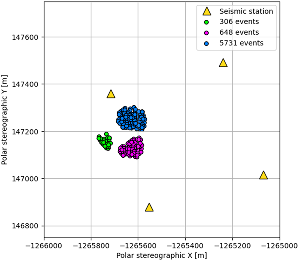


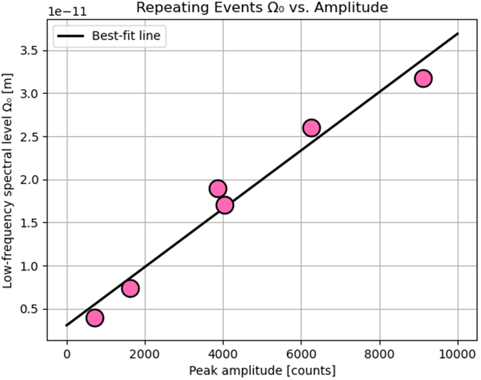


 Open access

